representation theory and invariant neural networks
TRANSCRIPT

N.U
Discrete Applied Mathelnatics 69 (I 996) 33-60
DISCRETE APPLIED MATHEMATICS
Representation theory and invariant neural networks ”
Jeffrey Wood *, John Shawe-Taylor
Received 5 April 1994; revised 19 December 1994
Abstract
A feedforward neural network is a computational device used for pattern recognition. In many recognition problems, certain transformations exist which, when applied to a pattern, leave its classification unchanged. Invariance under a given group of transformations is therefore typically a desirable property of pattern classifiers. In this paper, we present a methodology, based on representation theory, for the construction of a neural network invariant under any given finite linear group. Such networks show improved generalization abilities and may also learn faster than corresponding networks without in-built invariance.
We hope in the future to generalize this theory to approximate invariance under continuous
groups.
1. Introduction
A typical property of a pattern recognition problem is the invariance of the classi-
fication under certain transformations of the input pattern. By constructing the pattern
recognition system in such a way that the invariance is in-built a priori, it should bc
possible to speed training and/or improve the generalization performance of the system.
Numerous papers have been written on the subject of invariant pattern recognition
(see for example [6,10,17,19]), but few make use of the wealth of highly applicable
material in the field of group theory. [n this paper we apply standard representation
theory to obtain a number of interesting and general results.
For certain finite groups, namely permutation groups, invariance can be achieved by
building a Symmetry Network (see [ 13,151) in which connections share weights. This
work generalizes the theory of Symmetry Networks to the problem of invariance under
any given finite linear group.
,‘.This research was funded by the Engineering and Physical Sciences Research Council and the Defencc Research Agency under CASE award no. 92567042. @ British Crown Copyright 1995 /DR.4 Published with the permission of the Controller of Her Britannic Majesty’s Stationery Office.
* Corresponding author.
Crown copyright 0 1996 Published by Elsevier Science B.V. SSDI 0166-218X(95)00075-5

34 J. Wood, J. Shawe-Taylor I Discrete Applied Mathematics 69 (1996) 3340
We begin by presenting the necessary background in the field of neural networks. We
then summarize the theory of Symmetry Networks and introduce some representation-
theoretical notation. In Section 2 we introduce a new class of networks, Group Rep-
resentation Networks, and give a classification of group representations based on a
property which amounts to their degree of applicability in these networks. In Section3
we consider a special class of Group Representation Networks, namely Permutation
Representation Networks. In Section 4 we turn to other classes of Group Representa-
tion Networks. In Section 6 we discuss some practical issues and summarize the results
of some simulations. In Section 7 we conclude.
This paper is based on standard group representation theory. The results we use can
be found in most introductory texts on the subject, see for example [1,2,4].
1.1. Feedforward networks
In this section we summarize basic neural network terminology. For further infor-
mation, see the classic literature on the subject [7,&l l] or for an overall view of the
field see [3,5].
A feedforward neural network is a (finite) connected acyclic directed graph with
certain properties. Each edge (connection) of the network has an associated weight,
which is usually a real number. Each node (or neuron) of the network has an associated
function, the activation function which is a mapping from the real numbers to some
subset of the real numbers.
The inputs or input nodes of the network are those neurons with no connection
leading into them. The input nodes have no activation functions, or can be regarded as
having the identity function as an activation function. The outputs or output nodes of
the network are those neurons with no connection leading from them. The remaining
nodes are known as hidden nodes.
Neurons with the same connectivity are typically arranged in a layer. The input
nodes form one layer and the output nodes another. There may be one or more hidden
layers (layers of hidden nodes).
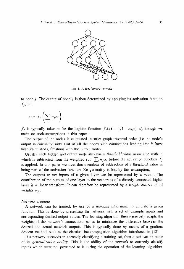
Fig. 1. shows a typical network, in which the neurons are grouped together in layers.
We have not fully connected those layers which have connections between them, since
this would have cluttered the diagram. The information flow in the network is from
the bottom of the figure upwards. This is a conventional manner of representation of a
network. Hence we refer to layer A as being higher than layer B if information flows
from B to A (though not necessarily directly). The output layer is clearly the highest
layer and the input layer the lowest. The functionality of the network is defined as
follows. The input of the network is a vector of real values which defines the output
of each input node. The output of the network is the vector of values which are the
outputs of each output node. The network’s output is computed as follows .
The net input of a given hidden or output node j is the weighted sum xi wjixi,
where the summation is done over all nodes i with connections leading to node j. Xi
denotes the output of node i and wjl denotes the weight of the connection from node i
J. Wood, J. Shawe-Taylor / Discrete Applied Mathematics 69 11996) 3340 35
Fig. 1. A feedforward network
to node j. The output of node j is then determined by applying its activation function
fj, i.e.
X.j = ,fj C WjiXi . it )
J; is typically taken to be the logistic function fi(x) = 1 /l + exp( -x), though we
make no such assumptions in this paper.
The output of the nodes is calculated in strict graph traversal order (i.e. no node’s
output is calculated until that of all the nodes with connections leading into it have
been calculated), finishing with the output nodes.
Usually each hidden and output node also has a threshold value associated with it,
which is subtracted from the weighted sum C, wjix, before the activation function ,f,
is applied. In this paper we treat this operation of subtraction of a threshold value as
being part of the activation function. No generality is lost by this assumption.
The outputs or net inputs of a given layer can be represented by a vector. The
contribution of the outputs of one layer to the net inputs of a directly connected higher
layer is a linear transform. It can therefore be represented by a weight matrix W of
weights w/i.
Network training
A network can be trained, by use of a learning algorithm, to emulate a given
function. This is done by presenting the network with a set of example inputs and
corresponding desired output values. The learning algorithm then iteratively adapts the
weights of the network’s connections so as to minimize the difference between the
desired and actual network outputs. This is typically done by means of a gradient
descent method, such as the classical backpropagation algorithm introduced in [12].
If a network succeeds in correctly classifying a training set, then a test can be made
of its generalization ability. This is the ability of the network to correctly classify
inputs which were not presented to it during the operation of the learning algorithm.

36 J. Wood, J. Shawe-TaylorlDiscrete Applied Mathematics 69 (1996) 3340
A network which fails to generalize well has not learned the target concept correctly,
but may succeed if further trained on a larger set of examples.
1.2. Symmetry Networks
The concept of a Symmetry Network was introduced in [13]. Essentially, a Sym-
metry Network is a feedforward neural network which is invariant under a group of
permutations of the input.
This invariance is achieved by extending each permutation from its natural action on
the input nodes to an automorphism of the network, i.e. a permutation of all network
nodes. Each automorphism has an obvious induced action on the connections of the
network. An automorphism is said to be weight-preserving if the weight of any two
connections in the same orbit is the same.
Formally, a Symmetry Network is a pair (M, 9), where JV is a feedforward network
and 99 a group of weight-preserving automorphisms of ~4’” which are required to fix
each output node. In addition we require that the activation function is fixed over each
node orbit (this is not a stringent requirement since it is usual to fix the activation
function over an entire network).
The output of a Symmetry Network is guaranteed to be an invariant under the action
of 9 on the input nodes.
Since the group of automorphisms is weight-preserving, any two nodes in a given
orbit have equivalent, if not identical, connectivities. Thus for convenience we associate
node orbits with network layers, although the correspondence is a little misleading. In
particular with this association each output node appears in a separate layer.
With each orbit (layer) we can associate a subgroup, namely the stabilizer of an
arbitrarily chosen node of that orbit. The nodes of the orbit are then naturally asso-
ciated with that subgroup’s cosets, the number of nodes in the layer being equal to
the subgroup’s index. This suggests a natural way to construct a Symmetry Network
under a given group Y; we choose a subgroup for each hidden layer. The subgroup
corresponding to the input nodes is determined by the action of 9 on the input nodes,
which is given by the problem in hand. The subgroup corresponding to each output
node is the whole group 9.
The connections between two given network layers are partitioned into orbits, two
connections in the same orbit being constrained to have equal weight. In [18] it is
shown that the orbits of network connections between layers associated with subgroups
9 and Z correspond precisely to the double cosets of the pair (9,.X’). Furthermore,
the correspondence is specifiable, which allows a relatively efficient construction of the
connection orbit structure.
Conventional learning algorithms can readily be adapted and applied to Symmetry
Networks. The only change in such algorithms is that the variable parameters of the
network are now the weights of the connection orbits, rather than the weights of the
connections themselves.

J. Wood, J. Shawe-TaylorlDiscrete Applied Malhemutics 69 (1996) 3340 37
One open issue in the subject of Symmetry Networks is that of discriminahility, i.e.
the ability of the network to discriminate between input patterns which are not in the
same orbit under the invariance group. This issue is discussed in the paper [ 151, where
examples of both fully discriminating and partially discriminating networks are given.
with reference to the graph isomorphism problem.
1.3. D+nitions and notation from representation theory
In this section we list some terminology and notation which we will use from the
field of representation theory.
We always denote our finite invariance group by 9, with ,Y? and 9 denoting sub-
groups. We use A, B and M to refer to completely arbitrary group representations.
P will be used to denote an arbitrary permutation representation and 2 an arbitrary
inversion representation (defined below).
Given a representation A, we write x(A) for its character. We denote the inner
product on characters over a group 9 or subgroup ,?P by (,)Q and (,).R respectively.
Given representations A and B of 9, we denote by A cx B the direct product of A
and B.
We refer to a homomorphism from representation A to representation B as meaning
a homomorphism from the (left) module under 3 associated with A to that associated
with B. All representations dealt with in this paper are assumed to be associated with
left modules. This is an arbitrary decision, consistency being the only requirement.
The space of homomorphisms from a module U to a module V is called the in-
tertwining space of (U, V) and its dimension the intertwining number of U and c’.
Since we deal with representations, rather than modules, we will refer instead to the
intertwining space and number of the corresponding representations.
For a representation A of a subgroup .Z of 3, we denote by ind$A the induced
representation of 3 from A. For a representation B of 3 and given a subgroup .P of
‘9, we denote by res$B the restricted representation of B to .#.
Let .# be a subgroup of 9. The jixed point subspace of .Z (in a given module I’
under 9) is the space of all vectors of V which are fixed by every element of .#
Finally we wish to make a non-standard definition. An inversion matrix or reflection
matrix is a diagonal matrix with diagonal entries of fl. An inversion representation
is a matrix representation in which all group representative matrices can be written as
the product of an inversion matrix and a permutation matrix.
2. Group Representation Networks
We have said that each layer of a Symmetry Network is associated with a subgroup
of the invariance group 3’. The action of 3 on the nodes of a layer is then equivalent
to its action on the cosets of the corresponding subgroup; i.e. the subgroup defines a
permutation representation of the invariance group.

J. Wood, J. Shawe-Taylor1 Discrete Applied Mathematics 69 (1996j 3340
It is possible to associate layers of the network with group representations which
are not permutations. This is a particularly useful technique to apply to the input layer
since it allows the construction of a network invariant under an arbitrary (finite) group
of linear transformations, as will be seen shortly.
We now formalize this concept, which requires a preliminary definition. We write
f to denote the extension of f : 172 H R to action on a vector of arbitrary dimension
(in the obvious componentwise manner).
Definition 2.1. Let A be an n-dimensional matrix representation of the group 9. Then
the function f : R! H R is said to preserve the representation A if
f(A(g)v) = A(g)&) v’v E RN, g E 9
Definition 2.2. A Group Representation Network (GRN) is a pair (JV, 9), where JV
is a feedforward network and the following conditions apply :
1. The nodes are partitioned into layers. With each layer is associated a representation
of 8, of dimension equal to the number of nodes in the layer. There are no intra-layer
connections.
2. Each output node is in a layer by itself, associated with the trivial representation.
The input nodes also form one or more layers.
3. The matrix of weights from a layer of nodes corresponding to representation A
to a layer corresponding to representation B is a homomorphism from A to B.
4. The activation function is fixed over a given layer and preserves the group rep-
resentation associated with that layer.
A Symmetry Network is a special case of a Group Representation Network in which
every layer’s associated representation is a permutation representation.
We now state and prove the result which forms the basis of this paper.
Theorem 2.3. The output of a GRN (X,9) is invariant under the action of 9 on
the input layer of Jlr.
Proof. We start by indexing the layers of JV” by 0, 1, . . . L, on the understanding that
there are no connections from a layer to any lower-indexed layer. Hence layer 0 is the
input layer and the output layers are those with the highest indices.
Let A, denote the matrix representation associated with layer i, fi the activation
function of layer i and yi(X) the vector of outputs from the nodes of layer i given x
as input to the whole network.
Let W(i,j) denote the matrix of weights of the connections leading from layer i to
layer j (thus j > i). W(i,j) will be the zero matrix for disconnected layers.
Now consider two network inputs xi and x2 which are related by a group transfor-
mation g E FJ. Let P(i) be the statement
We now prove P(i) for i E 0.. . L by induction on i.

J. Wood, J Shawe-TaylorlDiscrrte Applied Mathematics 6Y (1996) 3340 39
P(0) is true since Ya(x,) = x1 and Yo(x~) = x2 are the inputs of the network which
are related by transformation g according to the representation A*. Assume P(0) . . P(k )
are true; thus Ai(g)y;(x, ) = yi(x2) for all i E 0.. k. We now have:
4
k
yk+1(~2) = .f‘k;l c W(i, k + l)Y,(x~) i=O 1
(this is the functionality of the network)
k
c W(i, k + 1 )A,(g)y,(xl ) (by induction hypothesis)
\ r=O /
k
= f‘k+1 ( Ak+,(g) c WC&k + 1 )Y&I )
i=o
(W(i, k + 1) is a homomorphism from the representation A, to AR+, )
k
= Ak+l(dfk+l c W(i, k + 1)X(x1 )
i=o
(since J‘k +l preServesilk+ I )
= Ak+~(.q)Yk+~h).
Hence P( k + 1) is true.
By the principle of induction, P(L’) is true for all output layers L’, i.e.
.YL’(X2) = ALJ(g)YLt(xl)’
However, each output layer corresponds to the trivial representation, so Y~f(x2) =
YL,(x,) for all output layers L’. Hence any two inputs in the same orbit under 9 yield
the same output of 2”. !I!
We are now in a position to investigate the use of different representations in a
Group Representation Network. This requires some preliminary notation: For any real
number a, we define the following functions;
I,+& :IR~lfC,byZ,+(x)= Tndefined l,(x) = undefined. x > 0.
> ;$;
> Qx, x < 0.
Now we define a set of ‘nicely-behaved’ functions @ as follows:
@ = {d, : R H JR qb intersects 1,’ at an infinite number of places for at most one
value of a, and 4 intersects 1; at an infinite number of places for at most one value
of u}.
The following theorem provides a classification of all group representations according
to the functions in @ which preserve those representations.
Theorem 2.4. Let A be u jinite-dimensional representation of the group 99 ucting on
a reul vector space, ,f : R H R a function which is such thut ,f’o : R H R dejned hi
,fo(x) = f(x) -f(O) is in @. Then f preserves A f and only if one of the jtillowing
conditions holds :
1. A is a permutation representation.

40 J. Wood, J. Shawe-TaylorlDiscrete Applied Mathematics 69 (1996) 3340
2. A is an inversion representation and f is odd. 3. A is a unit-row representation (i.e. every row of every matrix of A sums to 1)
and f is a&e. 4. A is a positive representation (i.e. every entry of every matrix of A is non-
negative) and f is semilinear (i.e. there exist reals kl and kz such that f(x) = klx
for x 3 0, f(x) = kzx for x < 0).
5. f is linear.
The proof of this theorem appears in Appendix A. We note that most functions of
practical interest (with a few exceptions such as tanx) are in @.
Theorem 2.4 effectively provides a categorization of group representations into classes
which are preserved by different types of activation function. The reader should note
that, since subtraction of a threshold is being regarded as part of the activation hmc-
tion, thresholds cannot be used in neuron layers corresponding to representations other
than permutations and unit-row representations.
In Sections 3 and 4 we consider the use in a GRN of each of our named classes of
representation. Before that, however, we give some general results on the structure of
a single layer of connections in a GRN.
2.1. Weight matrix form
We now consider the structure of the connections between a given pair of layers
in a Group Representation Network. All the information about these connections is
contained in the weight matrix IV, which is the linear transformation that yields the
net input of the higher layer given the output of the lower layer. By the definition of
a GRN, W is a homomorphism from the representation of !9 associated with the lower
layer to that associated with the higher layer. Thus W is an element of the intertwining
space of the pair of representations concerned. We now state an explicit formula for
any weight matrix IV.
Lemma 2.5. Let A and B be two representations of group 9 (corresponding to left modules). Then any homomorphism W from A to B is of the form
W = j& ~B(g)XA(g-‘1 69
for a fixed matrix X, and furthermore any matrix of this form is a homomorphism from A to B.
Proof. Let W be a homomorphism from A to B. Hence
WA(h) = B(h)W
for all h E 9. Hence we find that X = W satisfies the equation of the lemma, so W is of the required form.

J. Wood, J. Shawe-TaylorlDiscrete Applied Mathematics 69 (1996) 33-60 41
Conversely, let W be of the form in the lemma. Now for all h E 9,
= & c WdW(g’-’ ) ( reor ermg the sum by setting 9’ = h-‘g) d <J’E?/
=B(h)W.
Hence W is a homomorphism from A to B. Cl
From Schur’s Lemma we immediately derive the following results for the special
case for when the representaiions we are concerned with are irreducible.
Lemma 2.6. Let A and B denote two representations corresponding to connected
layers of a Group Representation Network. Then we have the following results for
uny weight matrix W of the connections between the two luyers.
1. If A and B are irreducible and equivalent then W = kl .for some k E 1w.
2. If A and B are irreducible and inequivalent then W = 0.
Lemma 2.5 gives a formula for any valid weight matrix W. By using a matrix X
with independent variables as entries we obtain a completely general weight matrix W
in which each entry is a linear combination of the entries of X. We call this matrix the
generalized weight matrix of the pair (‘4, B) and denote it by WAJ. A specific weight
matrix is given by any mapping of the variables in X to the real numbers. Henceforth
when we refer to a weight matrix we will be referring only to a generalized matrix
as defined in this manner. Note that W ,4,B defines and is defined by the intertwining
space of (A,B).
Whilst the entries of X are linearly independent, the entries of W,Q will almost
always be expressible in terms of a smaller set of parameters. The minimum number
of parameters in terms of which the general weight matrix WA,J can be expressed is
the number of linearly independent weights. We refer to this number as the parameter
dimension p(A,B) of WQ. Hence p(A,B) is the intertwining number of A and B.
A standard result of representation theory is that the intertwining number of repre-
sentations A and B is equal to the inner product of the characters of A and B (see for
example [l]). Thus for our application of representation theory we obtain:
Lemma 2.7. Given any two representations A and B of 9, bve have
p(A, R) = MA), x(B)JY.
Another standard result is that the intertwining number of two permutation represen-
tations is the number of double cosets of the pair of subgroups corresponding to those
representations. This explains the connection between the connection orbits and double
cosets in a Symmetry Network.

42 J. Wood, J. Shawe-Taylor/ Discrete Applied Mathematics 69 (1996) 33-60
2.1.1. Direct product representation form
The formula of Lemma 2.5 expresses the weights as linear combinations of a set of
parameters. However this is not a very useful form for the formula. We rewrite it in
terms of the direct product of the representations A and B, this being the representation
of $9 defined by Y’s action on the network connections. To do this, we require a result
to do with the direct product of arbitrary matrices.
For an arbitrary m by IZ matrix X, let c(X) denote the mn-dimensional vector obtained
by writing the columns of X out one after another, to form a column vector. Similarly,
let r(X) denote the vector obtained by writing out the rows of X in a column vector
(not a row vector).
Lemma 2.8. Given W = BX4 where all matrices are arbitrary, we have
1. c(W) = (AT @ B)c(X),
2. r(W) = (B @ AT)r(X).
Here T denotes transpose and ~3 denotes direct product.
The proof of this result is lengthy but relatively simple and of no interest in its own
right. We therefore leave it to the reader.
We now apply this result to the formula of Lemma 2.5. We first assume that the
representations A and B are orthogonal; thus A(g)T = A(g-‘) for all elements g of 9.
The relationship we get is
We now introduce a new matrix @A$ by the formula
~K,B) = @A,Ldx), @A,B = i ,G, ~W@A(d.
CEY
(1)
We call the matrix @,Q the coe@cient matrix of the representations A and B. It defines
a mapping from the space of possible parameter matrices X to the intertwining space of
(A, B). @,Q can also be regarded as the mean value of the direct product representation
A @ B, which as a group average is naturally invariant under the action of any group
element.
The trace of QA,~ is the average character of the representation A @B over the whole
group. Since the character of A @B is equal to the product of the characters of A and
B, this trace is equal to (x(A),x(B)), which by Lemma 2.7 is the parameter dimension
of WA,B.
As remarked earlier, the parameter dimension of WA,B is the number of linearly
independent weights, which is clearly the rank of @A,B. Thus we have:
Lemma 2.9, The rank and trace of the coejficient matrix @A~J are equal to p(A,B).

J. Wood, J. Shawe-Taylor I Discrete Applied Mathemutics 69 11996J 3340 43
That the rank of @A,~ is equal to its trace is inevitable since @A,B is in fact a
projection matrix.
Note however that unless the coefficient matrix has full rank (which will not usu-
ally be the case), there will be redundant parameters. It would be useful to find an
expression for the weights in terms of a minimal set of parameters.
This can be done by column-reducing the matrix @A,B to Echelon form, which we
now define (following the definition given in [9]): Let A be an m by n matrix; let r,
denote the ith row of A which is not a linear combination of preceding rows. Then A
is said to be in column-reduced Echelon ji)rm if r, is equal to the ith row of the n by
n identity matrix for all i E 1 . . . rank(d). We define row-reduced Echelon form in an
analogous manner.
Now given any invertible matrix E (in particular an elementary matrix), E-‘r(X)
is still a vector of independent parameters. Thus we can write
where x = EI’E;’ .Ek-‘r(X) is a parameter vector and @A,B = @,QE~ E2E1 is
the column-reduced Echelon form of QA,~. This effectively expresses Y( W,4,~) in terms
of a parameter set with size equal to p(A,B).
3. Permutation Representation Networks
We now introduce a subclass of Group Representation Networks for which we can
simplify the results already presented.
Definition 3.1. A Permutation Representation Netn’ork CPRN) is a Group Represen-
tation Network in which every hidden layer (and trivially every output layer) corre-
sponds to a permutation representation.
Thus all Symmetry Networks are PRNs. The converse however is not true since a
PRN allows a non-permutation representation at the input layer. However the subnet-
work of a PRN formed by deleting the input layer and all connections leading from it
has the structure of a Symmetry Network.
Since we allow any linear representation to act on the input layer of a PRN, we
can build a PRN which is invariant under any finite linear group. The use of PRNs
rather than general Group Representation Networks therefore restricts the choice of
network structure but not the class of groups under which invariance can be achieved.
Also, recall from Theorem 2.4 that the use of permutation representations places no
restriction upon the activation functions that we can use.
For a PRN, it is relatively easy to build upon the theory presented so far. Again, as
in the case of a Symmetry Network, the hidden and output layers now correspond not
only to representations of the invariance group c!? but also to subgroups.

44 J. Wood. J. Shawe-Taylor f Discrete Applied Mathematics 69 (I996) 3340
3. I. Further notation and de$nitions
We therefore consider a given pair of layers corresponding to representations M and
P. Again we take these representations to correspond to left modules under 9. P cor-
responds to the higher layer and hence is a permutation representation. We furthermore
assume that it is transitive; if this is not the case then the higher layer can be split
up into distinct layers which do correspond to transitive permutation representations,
and these layers can be considered separately. The stabilizer of a node (we arbitrarily
choose the first node) in the higher layer is a subgroup of 9 which we denote by z@.
Let m denote the index of ~9’ in 9, and h,, hz,. . ., h, the right coset representatives of
2 (we take hl = e). M may or may not be a permutation representation; however we assume as before
that it is orthogonal. Let n denote the dimension of representation M. The action of 9 on the nodes of the higher layer corresponds to its action on the
right cosets of 2; thus
P(g)(ij) = 1 ++ Yfhig = Afhj.
Finally, we will find the following definition very useful.
(2)
Definition 3.2. Given a representation M of a group 9 with subgroup ~9, we define
the characteristic matrix J&‘(X) of the subgroup 2 (in the representation M) by the
equation
d(s) = k c M(h). hE.%
3.2. Reducing the parameter set
From Eq. (1) we have that
where the #ij’s are submatrices of C#QQ defined by
and r(X)T = (x:x:. . . xi), the xi’s being n-dimensional.
J. Wood, J. Shawe-Taylor I Discrete Applied Mathematics 69 (1996) 3360
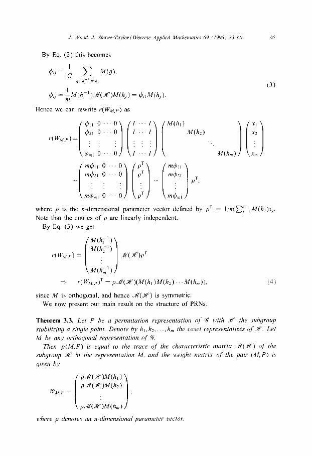
By Eq. (2) this becomes
k, = $j c M(g),
<!Eh ‘Xh,
Ct)lf = ~M(h;‘)eX(X)M(h,) = $11M(hj).
Hence we can rewrite Y( WM,~) as
I ”
I ”
. .
.
. .
I ..
PT
PT
PT
M(hl) M(hz 1
= -l m&l InqQ, m&l 0 0 0 ... “’ ... 0 0 0
T P 3
where p is the n-dimensional parameter vector defined by pT = 1 /m cl’=, M(h j )x,.
Note that the entries of p are linearly independent.
By Eq. (3) we get
4s
(3)
* ~V’M.P)~ = p~(~)(M(hl)M(h2)...M(h,)), (4)
since M is orthogonal, and hence AZ’(X) is symmetric.
We now present our main result on the structure of PRNs.
Theorem 3.3. Let P be a permutation representation of 9 with 2 the subgroup
stabilizing a single point. Denote by hl, h2,. . , h, the coset representatives of .F. Let
M be any orthogonal representation qf 99. Then p(M,P) is equal to the trace of the characteristic matrix A’(.X) of’ the
subgroup .F in the representation M, und the weight matrix of the pair (M,P) is
given by
W M.P =
p.A’(.%)M(h,)
p:,d(x)M(h2)
where p denotes an n-dimensional parameter vector.

46 J. Wood, J Shawe-Taylor1 Discrete Applied Mathematics 69 (1996) 3340
Proof. The formula for the weight matrix follows immediately from Eq. 4. We there-
fore have only to prove that p(A4,P) = Trace(A(Z)). By Lemma 2.7 we have
AMP) = (X(M)> X(P))9
= (X(M), X(ind$l ))g,
where 1 denotes the trivial representation of 2. That P = ind$l is a standard result.
By Frobenius’ Reciprocity Theorem we get
AMP) = Mres9OAl ))z
= Trace(A(%?)). 0
Thus we have written WM,P in terms of a parameter vector p, the characteristic
matrix A(%‘) and a set of coset representative matrices. Note however that whilst the
12 entries of p are linearly independent, the parameter dimension need not be n.
3.3. Properties of the characteristic matrix
We now analyze the characteristic matrix of a given subgroup 2. This matrix is
evidently of considerable importance since it determines the entire structure of the
weight matrix.
Theorem 3.4. Let A4 be an orthogonal representation of the group 9 associated with
left module V. Let .X be a subgroup of 9. Then &(A?) is a projection matrix onto
the fixed point subspace of ~6 in V.
Proof. We prove first that the range of A(%) is equal to the fixed point subspace of
X, and then that .,&Z(X) is a projection matrix.
1. First we show that the range of A?(X) is a subspace of the fixed point subspace
of 2. Let w = A(X)v for some v E V, h be any element of X’. Now we have
M(h)w = M(h)(A(X’)v) = (M(h)A’(X’))v = _M(X)v = w.
Thus the range of A#(&!) is a subspace of the fixed point subspace of A?.
Now let v be any vector in the fixed point subspace of 2; i.e. M(h)v = v Vh E 2.
Summing over X gives Jl(X)v = v; i.e. v is in the range of A!(X). Therefore the
range of A%‘(&?) is equal to the fixed point subspace of H.
2. Projection matrices are those which are both idempotent and self-adjoint. A!(X)
is idempotent:

J. Wood, J. Shawe-Taylor1 Discrete Applied Mathematics 69 (1996) 3340 47
.4’(X) is also self-adjoint (i.e. its transpose is equal to its complex conjugate), because
it is real, and also symmetric as A4 is orthogonal. Hence -A!‘(X) is a projection matrix.
This completes the proof of the theorem. 0
The above result is an extremely pleasing property of the characteristic matrix
Corollary 3.5. For orthogonal M, the trace of the characteristic matrix JZ(.#‘)
is equal to its rank, which is also equal to the dimension qf the fixed point suhspacr
of’ .x.
Proof. The eigenvalues of any projection matrix are 0 and 1. The trace of a matrix is
equal to the sum of the eigenvalues. The rank of a matrix is the number of non-zero
eigenvalues. The dimension of the fixed point subspace of 2 is the dimension of the
range of I&‘. Hence all three quantities are the same. D
It is helpful to view the parameter dimension as the dimension of the fixed point
subspace of .Y?+“. It is often easy to see what this value is. In particular the parameter
dimension will be n (the maximum possible) if and only if fl is the trivial subgroup.
The choice of the subgroup 2 is evidently crucial to the structure and power of
the resulting PRN. It therefore affects the discriminability and learning abilities of the
network, as will be discussed briefly in Section 6.
3.4. A minimal parameter set
We have a formula (in Theorem 3.3) expressing the weights in terms of a set of n
parameters. However we know that the parameter dimension is the rank of the subgroup
characteristic matrix, which is at most n and certainly will not be equal to n in general.
The question then arises as to how to express the weights of the network in terms of
a minimal parameter set.
The answer to this problem again lies in the reduction to Echelon form, this time
of the characteristic matrix. For if the matrices El, Ez,. . . , Ek define a sequence of
operations which convert A’(X) to row-reduced Echelon form, then
where J&‘(~~) = Ek . . E~E~JZ(S) is the Echelon form of A’(X) and p = pE, ‘ET ’
. EF’ is a new parameter vector. We can therefore replace p by p and A’(-X )
by A“(X) in the formula for the weight matrix given in Theorem 3.3. .&‘(.fl) will
contain a number of non-zero rows equal to p(M,P), and hence only the corresponding
parameters in p will be used in the formula for W.
Standard algorithms exist for reduction of a matrix to Echelon form. Thus the entire
process of calculation of a weight matrix in terms of a minimal set of parameters can
easily be automated.

48 J. Wood, J. Shawe-Taylor1 Discrete Applied Mathematics 69 (1996) 3360
4. Other representations
We now consider the further categories of group representations arising from Theo-
rem 2.4.
The second category of group representations which are preserved by a broad class
of activation functions is the inversion representations. We therefore deal with these
next.
4.1. Inversion representations
Recall an inversion matrix is a diagonal matrix with diagonal entries of fl. An
inversion representation is a matrix representation in which all group representative
matrices can be written as the product of an inversion matrix and a permutation matrix.
In effect, then, each representative matrix in an inversion representation is a permutation
matrix in which some of the l’s may have been replaced by - 1 ‘s. Like permutation
representations, inversion representations are always orthogonal.
We let Z denote an arbitrary inversion representation. For any g E 3, we can
decompose Z(g) into an inversion matrix $(g) and a permutation matrix P(g) :
Z(g) = b4g)fYg)
For convenience we write Z = I,IJP. It is easy to see that P is also a representation
of 9.
We are now able to provide a classification of inversion representations Z = $P for
which P is transitive. When P is not transitive, we can rewrite Z as the direct sum
of inversion representations which do have transitive associated permutation represen-
tations. We can then consider each subrepresentation separately.
Theorem 4.1. Let Z = $P be an inversion representation with P transitive of di-
mension m. Let S = {-l,-2 ,..., -m,1,2 ,..., m) denote a set on which Z acts by
permutation in the natural manner.
Define a subgroup 3 of 3 :
2% = {g E gig(l) = fl}.
Then one of two cases holds:
1. Z is induced from a non-trivial alternating representation of the subgroup 3’,
and S forms a single orbit under Z.
2. Z is equivalent to P and partitions S into two orbits, either i or -i being in
each orbit for all i E 1 . . m.
Proof. We give only a sketch of the proof here. Since P is transitive, either i or -i
must be in the same orbit as 1 for all i, and the other must be in the same orbit as
- 1. The orbits of 1 and - 1 may or may not be distinct, but they clearly cover S, and
so there are either one or two orbits of S under Z.

J. Wood, J. Shawe-Ta$or I Discrete Applied Mathematics 69 11996) 3340 4’)
1. Assume S is a single orbit under Z. Define the class function x on .# by x(h) =
Z(h)(l.l) = 311 for all h E .7?.
It is easy to show that x is an alternating representation of .Yfu; furthermore it is
non-trivial since 1 and - 1 are in the same orbit. Let ind’ccc denote the representation
of 9 induced from a.
Let hl,h2,. . .,h, denote the coset representatives of 9, ordered so that hi( I ) = hi
for all i.
By the definition of an induced representation we get
It can be shown that Z(hjghi’)(l,l, = Z(g)(i,j,. Thus we get that ind$z = Z, which is
our required result.
2. Now assume S is partitioned into two orbits under Z. Define the matrix T by
0 if if j,
TCI. j) = 1 if i is in the same orbit as 1,
- 1 if i is in the same orbit as - 1
For any g E 9 we now get
This last step follows by consideration of the definition of T. Thus we get that
TZ(g)T-’ = P(g) for all y E 3, i.e. P is equivalent to Z. 3
When Z falls into the first category of inversion representations listed in the theorem.
we refer to it as a one-orbit inversion representation. Otherwise we call Z a two-orbit
inversion representation.
Having divided the inversion representations into two subclasses, we are now in a
position to give formulae for the parameter dimension and weight matrix of a pair
(M,Z), where M is an arbitrary orthogonal representation of 9.
Corollary 4.2. Let Z = $P he an inversion representation of group 9, ,c-ith P tran-
sitive. Let M be un arbitrary orthogonal representation of 9. Define two subgroups
,P, .#‘; of‘ 3 by :
-p={gE:q I g(l)=fl}, .F={gE9 / g(l)= I}
according to the action of Z on the .xet {-l,-2 ,... -m,1,2 ,... m}. Let hl,hz ,.,, h,
denote the right coset representatives of 2, ordered so that h,(l) = xki ,fbr all
i E 1 .m. Let J‘l, f2,. . f2,,, denote the coset representatives of 9, ordered so thut
,fi( 1) = i. .fm+( = -i for i E 1 . .m.

50 J. Wood, J. Shawe-Taylor1 Discrete Applied Mathematics 69 (1996) 3340
Then we have.
1. If Z is a one-orbit representation, p(M, Z) is Trace(M(F)) - Trace(A(%‘)),
and
i
P~(~W(fl> - Wfm+l>)
P~(mvfu-2) - M(fm+z)) W,z =
P~(~ML) - Mfzm>) 1.
2. If Z is a two-orbit representation, p(M,Z) is the trace of the characteristic matrix J&‘(Z) of 2 in the representation M, and the weight matrix is given by:
where qi = i 1; qi = 1 zf i is in the same orbit as 1,
where p is a vector of independent parameters.
Proof. Again we give only a sketch proof, considering each of the two cases in turn.
1. Suppose Z is a one-orbit representation. By Theorem 4.1, Z = ind$a for a
non-trivial alternating representation a of 2. Let res>A denote the restriction of rep-
resentation A of 9 to the subgroup X. For any representation A, let x(A) denote its
character. By Lemma 2.7 and Frobenius’ Reciprocity Theorem we have
P(M>Z) = k(M), x(Z)),
= k(M), z(ind$))g
= L&&M), ~4%
= & c 4hV’rMh)) hEZf
. = Trace( A( F)) - Trace( Jl”e( X)).
Now let P’ denote the permutation representation corresponding to subgroup 9 of $9,
i.e. F is the stabilizer of a point under P’. It can be shown that
p’(g) = i P(g) + Z(g) P(g) - Z(g)
2 ( P(g) - Z(g) P(g) + Z(g) >
Defining D = (( 1 - 1 )@lm), where @ denotes direct product and I, is the identity matrix
of degree m, we find DP’(g) = Z(g)D for all g E 9. Using the formula in Lemma
2.5, we can show that WMJ = DWM~,. By Theorem 3.3 we obtain the required result.
2. Suppose Z is a two-orbit representation. By Theorem 4.1, Z is equivalent to P. By Lemma 2.7, p(A, B) = p(A, C) whenever B and C are equivalent representations.
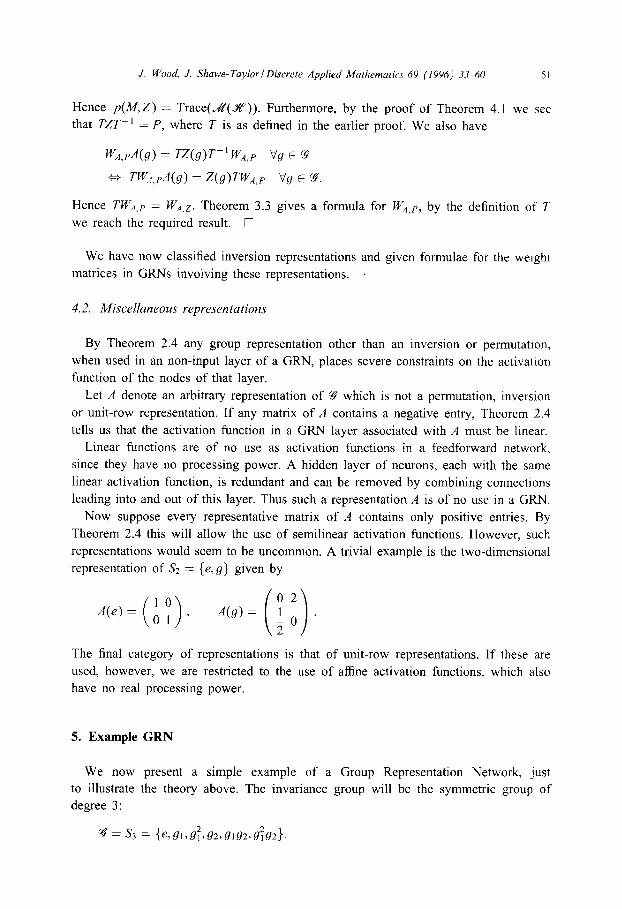
J. Wood, J. Shawe-Taylor i Discrete Applied Maihematic,s 69 (1996) 3340 51
Hence p(M,Z) = Trace(&(&‘)). Furthermore, by the proof of Theorem 4.1 we see
that TZT-’ = P, where T is as defined in the earlier proof. We also have
WA,PA(B) = WgY-’ WA,P vg E ‘w
@ TW,l.d(g) = Z(g)TWA,p v(J E 3.
Hence TV,,, = WA,~. Theorem 3.3 gives a formula for WA,~, by the definition of T
we reach the required result. 0
We have now classified inversion representations and given formulae for the weight
matrices in GRNs involving these representations. .
4.2. Miscdlaneous representations
By Theorem 2.4 any group representation other than an inversion or permutation,
when used in an non-input layer of a GRN, places severe constraints on the activation
function of the nodes of that layer.
Let A denote an arbitrary representation of 9 which is not a permutation, inversion
or unit-row representation. If any matrix of A contains a negative entry, Theorem 2.4
tells us that the activation function in a GRN layer associated with A must be linear.
Linear functions are of no use as activation functions in a feedforward network,
since they have no processing power. A hidden layer of neurons, each with the same
linear activation function, is redundant and can be removed by combining connections
leading into and out of this layer. Thus such a representation A is of no use in a GRN.
Now suppose every representative matrix of A contains only positive entries. By
Theorem 2.4 this will allow the use of semilinear activation functions. However, such
representations would seem to be uncommon. A trivial example is the two-dimensional
representation of 5 = {e, g} given by
The final category of representations is that of unit-row representations. If these are
used, however, we are restricted to the use of affine activation functions, which also
have no real processing power.
5. Example GRN
We now present a simple example of a Group Representation Network, just
to illustrate the theory above. The invariance group will be the symmetric group of
degree 3:

52 J. Wood, J. Shawe-Taylor I Discrete Applied Mathematics 69 (1996) 3340
We will build a four-layer network. The representations corresponding to each layer
are as follows.
1. The input layer corresponds to the two-dimensional irreducible representation As,
which is the representation obtained by regarding gr as a 120” rotation about the origin
and g2 as a reflection in the y-axis, action being on the Euclidean plane.
1 J5
Aok >
Ao(g2)
-1 0
= k-_) $ 21 = ’ ( o 1 > 2 2
2. The first hidden layer corresponds to an inversion representation Al induced from
the alternating representation of the subgroup {e,gz} :
A,(a)= (-I=), Al&)= (-;_;-;).
3. The second hidden layer corresponds to the regular representation AZ.
A&l 1 = 100000
000010 ’ A&2 I=
000001
000100
010000
001000
4. The output layer corresponds to the trivial representation A3 of 97.
Thus the numbers of nodes in each layer are 2,3,6 and 1 respectively. We take each
layer to have connections leading only to the layer above. The activation functions
involved are arbitrary, save that those in the first hidden layer must be odd.
By applying Theorem 3.3 and Corollary 4.2 we find the number of parameters in
each layer:
p(Ao,Ar) = 1, P(AI,Az) = 3, P(Az,A~) = 1.
We can also calculate the generalized weight matrices :
WA,,,A, = , WA,,Al =
u2 u3 a4
-a3 a4 -82
-a4 -a2 x3
-cc2 -cx4 -a3
@4 --cI3 a2
u3 a2 -u4 1 > WAz,A, =
Here the free parameters of the network are {al,. . , Q}. Additional degrees of freedom
can also be incorporated, for example by the addition of a variable ‘threshold’ to the
activation functions in the second hidden layer and the output layer.

J. Wood, J. Shawe-Taylor I Discwte Applied Mathemcrtics 69 (1996) 3340 5.3
The GRN specified above will be invariant under the action of Aa on the input
layer.
6. Practical issues
As with Symmetry Networks, Group Representation Networks may have a problem
with discriminability. We say that a network discriminates perfectly over a group 9 if
any two inputs which are in distinct orbits under 9 can also be distinguished by the
network. Discriminability is a property of a particular network structure, rather than
one of the invariance problem itself. Intuitively, we expect perfect discriminability to
be more common in networks with a greater number of free parameters. Experimental
observations have supported this conjecture.
Consider a problem which can be specified by the classification of a finite number
of orbits under group 9 (those inputs not in these orbits implicitly receiving a distinct
classification). A perfectly discriminating GRN can perform this pattern classification
without the need of training, which clearly saves a lot of computational time. This is
done simply by comparing the output of the network for a new (test) pattern with the
outputs of the prototype (training) patterns.
We also save computational space owing to the fact that the classification of an orbit
is given by the classification of a single input in that orbit. A conventional feedforward
network learning the same problem would require the classification of a number of
inputs in the orbit (the interpolative abilities of the network hopefully extending the
classification to the whole orbit).
In most practical problems, some degree of generalization will be required of the
network. The network must then be trained on a well-chosen set of prototype patterns.
Any standard learning algorithm (for example backpropagation) can be readily adapted
to reflect the fact that it is the parameters of the network’s weights that are adaptable,
rather than the weights themselves.
We also expect a GRN to train faster and/or to generalize more successfully than a
network without in-built invariance. This is simply because we are giving the network
information a priori and therefore it inevitably knows more about the problem than a
conventional network which would in effect have to learn the invariance in order to
generalize equally well. In [14], the generalization properties of Symmetry Networks
are investigated. Since GRNs are simply more general versions of Symmetry Networks,
we expect similar properties to hold for them.
6.1. Simulutions
In [ 131, a number of experiments were carried out using Symmetry Networks on
the graph isomorphism problem. In these experiments the Symmetry Networks trained
significantly faster than networks without in-built invariance.

54 J. Wood, J. Shawe-Taylor I Discrete Applied Mathematics 69 (1996) 3340
Since the development of the theory in this paper, we have performed two further
sets of experiments comparing the performance of GRNs with that of conventional
feedforward networks. Firstly, we tested a class of GRNs on the parity problem, where
the classification of a string is invariant under the inversion of an even number of
bits. The inputs were *l-valued; hence such an inversion is a linear transformation of
the input. We were able to present the problem to an invariant net by just two input
samples (one positive, one negative); the invariance specified the remaining classifica-
tions. Simulations showed that the invariant networks trained significantly faster than
conventional networks; the learning algorithm however sometimes failed to converge
with the in-built constraints of the GRNs.
A second experiment was carried out on a simple character recognition problem,
with invariance under 30” rotations and a vertical reflection. Seventy-two letters (with
classifications A, M and X) were presented as training data, each specified by the
coordinates of its key points. In this experiment, the invariant network was slower to
train than the conventional network. However it correctly classified new inputs 100%
successfully, whereas the conventional network achieved only 92% correct classifica-
tion.
7. Conclusions
We have introduced the concept of Group Representation Networks. These are feed-
forward neural networks which are intrinsically invariant under the action on the input
of an arbitrary finite linear group. GRNs include as a subclass Symmetry Networks,
which have previously been used to achieve permutation invariance.
The structure of a GRN is determined by a choice of representation for each layer
of the network. We have presented a classification of group representations according
to their usefulness in these new networks. We have analyzed the local structure of
GRNs employing the more applicable classes of representation. In particular we have
presented formulae for the number of free parameters and the weight matrix of a given
layer of connections in a GRN.
Appendix A: Proof of Theorem 2.4
For convenience we restate the theorem and its prerequisite definitions. For any real
number a, we define the following functions:
I,‘, 1, : R H lR, by Z,+(x) = yndefined Z,(x) = undefined, x > 0,
> ; “, “d
> a, x < 0.
Sp = (45 : R H lRJ$ intersects 1: at an infinite number of places for at most one
value of a, and # intersects I, at an infinite number of places for at most one value
ofa}

J. Wood, J. Shawe-TaylorlDiscrete Applied Mathematics 69 (1996) 3340 55
Theorem 2.4. Let A be a finite-dimensional representation of the group 97 acting on
a real vector space, f : R H R a function which is such that fo : R H R dejined by
,f’o(x) = f(x) - f(0) is in @. Then f preserves A tf and only tf one of the jollo~~ing
conditions holds :
1. A is a permutation representation.
2. A is an inversion representation und f is odd.
3. A is a unit-row representation (i.e. every row of every matrix of A sums to 1)
und f is u$fke.
4. A is a positive representation (i.e. every entry of every matrix of A is non-
negative) and f is semilinear (i.e. there exist reals kl and k2 such that ,f(x) = k1.x
fbr x 3 O,J‘(x) = klx for x < 0).
5. f is linear.
Before starting on the main body of the proof we present a number of preliminary
lemmas. Throughout, A denotes a finite-dimensional representation of the group 97
acting on a real vector space, and n denotes the dimension of A.
Lemma A.1. [f A4 is an invertible matrix which cannot be written us the product
of inversion and permutation matrices, then either M contains an entry other than
- 1,0,1 or else A4 contains a row with at least tw’o non-zero elements.
Proof. Let M denote an invertible matrix which contains no row with more than one
non-zero element and no entries other than - 1,0 and 1. No row of M can be all-zero,
and no two rows of M can be linearly dependent. Thus every row of M must contain
exactly one non-zero entry and similarly for every column. We can therefore write
M = MtM2, where Mt is diagonal with entries of 1 in rows where M has entries of
1 and entries of -1 in other rows. Ml will have zero entries in the same places as
M and 1 entries elsewhere. Thus MI is an inversion matrix and M2 a permutation
matrix. 0
Lemma A.2. If A is a positive representation, then any matrix M of A must have
exactly one (positive) entry in each row and column.
Proof. Let the inverse of M be denoted by N; N is in the representation A and hence
must itself have only positive entries. Considering the entries of the product MN = 1.
we have
Vi, j with i # j c MtkNkj = 0.
k=l
Now choose an arbitrary value of i. The ith row of M must contain a non-zero
element Mir (or else it would not be invertible). This we know is positive, and so
by the above formula we must have Nrj = 0 for all j # i. Since the rth row of N
cannot be all zero, we must have Nri # 0. But from this we conclude similarly that
56 J. Wood, J. Shawe-Taylor IDiscrete Applied Mathematics 69 (1996) 3340
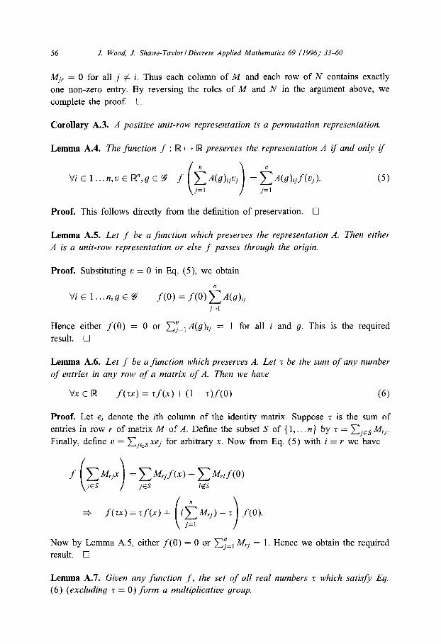
M_r = 0 for all j # i. Thus each column of M and each row of N contains exactly
one non-zero entry. By reversing the roles of M and N in the argument above, we
complete the proof. q
Corollary A.3. A positive unit-row representation is a permutation representation.
Lemma A.4 The function f : R H R preserves the representation A if and only tf
Vi E 1 . ..n.v E R”,g E 29 f = 2 A(nlij.f(VjJ (5)
j=l
Proof. This follows directly from the definition of preservation. 0
Lemma A.5. Let f be a function which preserves the representation A. Then either
A is a unit-row representation or else f passes through the origin.
Proof. Substituting II = 0 in Eq. (_5), we obtain
Vi E 1 . ..n.g E 9 f(0) = f(O)kA(g), j=l
Hence either f (0) = 0 or c/“=l A(g)ij = 1 for all i and g. This is the required
result. 0
Lemma A.6 Let f be a function which preserves A. Let z be the sum of any number
of entries in any row of a matrix of A. Then we have
\Jx E Ii3 f (TX) = zf (x) + (1 - z)f(O) (6)
Proof. Let ei denote the ith column of the identity matrix. Suppose z is the sum of
entries in row r of matrix M of A. Define the subset S of { 1,. . n} by z = Cjrs I&;.
Finally, define v = cjCsxej for arbitrary x. Now from Eq. (5) with i = r we have
f CM,j” =C”rjf(x)+CMrtf(o)
( 1 j&s j&s t&s
* f (0).
Now by Lemma AS, either f (0) = 0 or Cl=t Mrj = 1. Hence we obtain the required
result. 0
Lemma A.7. Given any function f, the set of all real numbers z which satisfy Eq.
(6) (excluding 7 = 0) form a multiplicative group.

J. Wood, J. Shawe-Taylor I Discrete Applied Mathematics 69 (1996J 3340 57
Proof. Let T denote the set of solutions z to equation (6). The associativity axiom
follows trivially, and the identity axiom can be verified by substituting z = 1.
Let 51, ~52 be in T. Now for any x E R we have
.f(~lW) =71f(zzx) +(1 - ~l)f(O)
= TI [TZf(X) + (1 - z2)J‘(O)l+ (1 - 71 V(O)
=z,z2f(x> +(I - 7172)f‘(O).
Hence Eq. (6) is satisfied for z = zlr2, and so T is closed under multiplication.
Finally, the proof that T is closed under inversion follows by rearrangement of
Eq (6). n
Lemma A.8. Let 4 : R H IF8 be a function in the set @. Suppose there exists a ualur
of T not in {-l,O,l} such that
vx E R a=) = Mx). (7)
Then 4 is semilinear. Furthermore, if there exists such a z lvhich is negatice, qij i.5
linear.
Proof. Let a denote a real value for which I,’ intersects 4, and let x1 denote a given
point of intersection, i.e. Zz(xl ) = $(x1 ). Now we have
&2X,) = 22&x,) = 221,+(X1) = 22CzY.l = l,+(r2x,)
(the last step since z2xl > 0). Hence zxl is another point of intersection. Similarly,
~~‘xi is a point of intersectionfor all z E Z. Hence if C# intersects 1: at all, it intersects
it at infinitely many points.
From this, since C$ is in @ we conclude that 4 intersects 1,’ for at most one value
of a, and clearly therefore for exactly one value, al say. Therefore for positive .r we
have 4(x) = l;(x). Similarly, we can deduce that for negative x and for some a2 t R
we have 4(x) = I;(x). Finally, for x = 0 it is clear that 4(x) = 0. We have effectively
deduced that b, is semilinear.
For the second part of the proof, we assume that 7 is negative (7 # -1). From the
equation for a semilinear function we obtain expressions for I and z@(x). Equating
these, we see that al = a2, i.e. f is linear. 0
We now begin the main body of the proof of Theorem 2.4.
1. Let A be a permutation representation. Then each row of A(g) contains exactly
one non-zero entry, which is 1. Thus Eq (5) holds trivially for every i and any ,f.
2. Let A be an inversion representation. Hence any group representative matrix in
A is the product of an inversion matrix and a permutation matrix. Any f preserves
all permutation matrices; hence f preserves A if and only if it preserves the inversion
matrices forming the matrices of A.

J. Wood, J. Shawe-Taylor1 Discrete Applied Mathematics 69 (1996) 3340
Therefore let A4 be such an inversion matrix, A4 # I. A4 must contain an entry of
- 1, and hence by Lemma A.6 we have
kfx E [w f(-x) = -f(x) + 2f(O).
However, since A is clearly not a unit-row representation, by Lemma A.5 we know
f(0) = 0, and hence we have that f is odd. The converse, that any odd function
preserves any inversion matrix, is easy to prove.
3. Let A be a representation which is neither an inversion nor a permutation repre-
sentation. We will consider the remaining cases simultaneously. We assume A contains
a matrix M which is neither an inversion nor a permutation (nor a product of the two).
By Lemma A. 1, there are two cases to consider regarding the entries of M:
(a) Assume M contains an entry M, not in {-l,O, l}. By Lemma A.6, Eq. (6)
holds for z = M,,.
(b) Conversely, assume M contains only entries of - 1, 0,l. Hence it contains a row
with at least two entries of *l. Choose two of these entries, M, and Mrt, if possible
such that they are both 1. We now have again two possibilities:
(i) M, = MyI = 1. In this case, we can apply Lemma A.6 and obtain Eq. (6) with
z = M, + M,., = 2.
(ii) At least one of the entries M, and M,., is - 1. However, now A is certainly
not a unit-row representation, since if it were, any entry of -1 in a row of M would
necessitate at least two entries of +l in that row, which would be a contradiction.
Therefore by Lemma A.5, f(0) = 0, and by Lemma A.6 we have Eq. (6) for r = -1,
i.e. f is odd. Hence we can say f(M,x) = M,f(x), f(M,,x) = M,,f(x).
Now we substitute v = M,xe, + Mrtxet (for arbitrary x) and i = r in Eq. (5) and
obtain
f<M:x + M;x) = Msf(Mrsx) + MrtfWrtx) + f(O) f: M, j=O, jfs, f
+ f(2x) =2f(x) + f(O) 2 Mrj j=O, jfs, t
= 2f(x) + (1 - 2)f(O) (since f(0) = 0).
Thus, in either case, Eq. (6) holds for T = 2.
At this stage, we have found a value k not in {-l,O, 1) such that Eq. (6) holds for
z = k. Recall that the function fs is defined by fs(x) = f(x) - f(0). From this we
derive the following:
Vx E [w fo(h) = kfo(x). (8)
Hence we can apply Lemma A.8 for 4 = fo E @‘, and so fo must be a semilinear
function. We now have the following two possibilities:
(a) A is a positive representation. By Corollary A.3, A cannot be a unit-row repre-
sentation and thus, by Lemma A.5, f(0) = 0, i.e. fo = f and f is semilinear.
J. Wood, J. Shawe-Taylor1 Discrete Applied Mathematics 69 (IYY6) 3340 59
We must also show that any semilinear function preserves any positive representation.
This follows from Lemma A.2; we can see that a sufficient condition for ,f to preserve
A is that f(a) = of for all x E R, c( E IR, CY > 0, which is equivalent to
semilinearity.
(b) A is not a positive representation. Then either k itself is negative and not equal
to - 1, or else k is positive and not equal to 1. In the latter case, let 1 denote a negative
element of some matrix of A. By Lemma A.6, we have Eq (6) for z = 1, and hence,
by Lemma A.7, this equation also holds for T = kl. Both 1 and kl are negative, and
at least one is not equal to -1.
So we have a negative value of r, other than -1, for which Eq. (6) and hence Eq.
(8), holds. By Lemma A.8 J‘o must be linear.
If A is a unit-row representation, we have effectively deduced that ,f’ must be afhne.
On the other hand, if A is not a unit-row representation, we have j’o = ,f‘ and thus ,f’
is linear.
It is evident that any linear function preserves any representation, hence the only
remaining part of the proof is to show that any affine function preserves any unit-row
representation. This is not hard, and we omit it for brevity.
This concludes the proof.
References
[I] M. Clausen and U. Baum, Fast Fourier Transforms (Wissenschaftsverlag, Mannheim 1993)
[2] P.M. Cohn. Algebra, Vol. 2 2nd ed., (Wiley, Chicester, 1989).
[3] L. Fausett. Fundamentals of Neural Networks (Prentice-Hall, Englewood Cliffs, NJ, 1994).
[4] W. Fulton and J. Harris, Representation Theory (A First Course) (Springer, New York, I991 ).
[5] J. Hertz, A. Krogh and R. Palmer, Introduction to the Theory of Neural Computation (Addison-Wesley.
Redwood City, CA, 1991).
[6] Y. Li, Reforming the theory of invariant moments for pattern recognition, Pattern Recognition 2.5 (7)
(1992) 723-730.
[7] W. McCulloch and W. Pitts, A logical calculus of the ideas immanent in nervous activity. Bull. Math.
Biophys. 5 (1943) 115-133.
[8] M. Minsky and S. Papert, Perceptrons (MIT Press, Cambridge, 1969).
[9] C.W. Norman, Undergraduate Algebra (A First Course) (Clarendon Press, Oxford, 1986).
[toI
[1 11 [I21
[I31
[I41
[I51
[I61
[I71
S. Perantonis and P. Lisboa, Translation, rotation and scale invariant pattern recognition by high-order
neural networks and moment classifiers, IEEE Trans. Neural Networks 3 (2) (1992) 241-2.51.
F. Rosenblatt, Principles of Neurodynamics (Spartan, New York, 1962).
D. Rumelhart, G. Hinton and R. Williams, Learning representations by back-propagating errors. Nature
323 (1986).
J. Shawe-Taylor, Building symmetries into feedforward networks, Proc. of First IEE Conference on
Artificial Neural Networks (1989) 158-l 62.
J. Shawe-Taylor, Threshold network learning in the presence of equivalences. in: Proceedings of NIPS-4
( Morgan Kaufmann, San Mateo, 1992).
J. Shawe-Taylor,Symmetries and discriminability in feedforward network architectures. IEEE Trnns
Neural Networks 4 (5) (1993) 816826.
J. ShaweTaylor and D. Cohen, The linear programming algorithm, Neural Networks 3 ( 1990)
575-582.
L. Spirkovska and M. Reid, Robust position, scale and rotation invariant object recognition using
higher-order neural networks, Pattern Recognition 25 (1992) 975-985.

60 J. Wood, J. Shawe-Taylor1 Discrete Applied Mathematics 69 (1996) 3340
[18] J. Wood and J. Shawe-Taylor, Theory of symmetry network structure, Technical Report, Department
of Computer Science, Royal Holloway, University of London (1993).
[19] C. Yuceer and K. Oflazer, A rotation, scaling and translation invariant pattern classification system,
Pattern Recognition 26 (5) (1993) 687-710.