1

Representative Input Parameters for Geostatistical Simulation

Michael J. Pyrcz (mpyrcz@ualberta.ca) Department of Civil & Environmental Engineering

University of Alberta

Emmanuel Gringarten (gringarten@earthdecision.com) Earth Decision Sciences, Houston, Texas, USA

Peter Frykman (pfr@geus.dk) Geological Survey of Denmark and Greenland (GEUS), Copenhagen, DENMARK

Clayton V. Deutsch (cdeutsch@ualberta.ca)

Department of Civil & Environmental Engineering University of Alberta

Abstract

Geostatistical simulation techniques are increasingly being used to create heterogeneous realizations for flow modeling and to assess uncertainty in hydrocarbon resources/reserves. These geostatistical simulation techniques reproduce the input statistics within ergodic fluctuations. The input statistics representing various model parameters must be computed from data that is representative of the entire domain being modeled. Geostatistical simulation does not accommodate a lack of representativeness in the data. Moreover, the extent to which the input statistics are reproduced depends almost exclusively on the size of the modeling domain relative to the range of spatial correlation; fluctuations in realizations of the full reservoir model do not depend entirely on the uncertainty of the input statistics. It is necessary to explicitly incorporate the uncertainty of the input statistics because they have a much larger and more realistic impact on the uncertainty of the full reservoir model than stochastic fluctuations. Best practices for determining representative input values of model parameters and quantification of their uncertainty are presented in this chapter.

Introduction The combinatorial space of uncertainty in reservoir modeling is inconceivably

vast. Local well data measure less than one trillionth of a typical reservoir volume. Seismic data provides excellent coverage, but its scale of measurement is very large and it must be calibrated to reservoir properties using limited well data. Reservoir models are often not adequately constrained by local well data. The choice of a geostatistical modeling approach and the values specified for the associated input model parameters

2

provide the most significant constraints on the modeling results. It is essential that the input statistics be representative of the entire domain being modeled.

Histograms and other statistical characteristics must be assembled from the local well data and often supplemented by outcrop studies and analog field data. However, wells are not drilled to be statistically representative and core data are not always taken uniformly from good and poor quality reservoir rock. The geostatistical modeler must take great care to assemble values of the model parameters that are derived from representative data.

Impact of the Histogram

To demonstrate the importance of adequately specifying the input histogram of a reservoir property such as porosity, consider the four wells shown in Figure 1. These wells are located in the North Cowden Field in West Texas where 62 wells have been drilled (the data were kindly provided by Amoco Oil Company, now part of British Petroleum, as an industry training set for the development of geostatistical methodologies). Porosity is given in units of percent averaged over the vertical thickness of the reservoir. The histogram on the right side of Figure 1 characterizes the vertical average of porosity for the 62 wells. The four wells have been randomly chosen to provide realistic local conditioning for the geostatistical realizations of porosity.

Note that the observed porosity distribution appears to be bimodal (see right of Figure 1). This indicates the presence of two distinct facies types—dolomite and siltstone. In practice, the two facies should be treated independently; however, this needs not be done for the purpose of the present discussion.

The mean of the vertical average porosity (henceforth referred to as average porosity) of the 62 wells is 8.4%. Two realizations constructed with sequential Gaussian simulation (SGSIM) using the reference (base case) histogram and the four wells as conditioning data are shown in the center of Figure 2. An isotropic semivariogram is used to fit the experimental normal scores semivariogram of the set of 62 wells based on a spherical model with a range of 3000 feet. The histogram in the top center is the observed base case histogram of average porosity. The histogram in the bottom center characterizes the resulting distribution of pore volume over 101 realizations. The units of pore volume are millions of cubic feet, assuming an average reservoir thickness of ten feet. Note the uncertainty in pore volume due to fluctuations among the realizations.

Considerable uncertainty exists with regard to the true distribution of average porosity. Consider three estimates of the distribution of average porosity, with associated means of 7.5%, 8.4% and 10%. These estimated distributions are shown on the top of Figure 2. Each of these estimated distributions were applied as reference distributions to calculate 101 realizations with sequential Gaussian simulation (two realizations of each case are shown in Figure 2). Although all 101 realizations are constrained to the data in the four wells shown in Figure 1, the estimated porosity distribution has a first order impact on the estimate of pore volume. A low case is shown on the left of Figure 2. This case represents an eleven percent reduction in mean average porosity, which translates to

3

a five percent reduction in mean pore volume compared to the base case (the histogram of pore volume resulting from the 101 realizations is shown in the lower left of Figure 2). The right side of Figure 2 shows the high case based on a mean average porosity of 10%. The histogram of pore volume resulting from 101 realizations is shown in the lower right of Figure 2. The small number of wells and the relatively large range of correlation dampen the effect of the change in mean porosity (twenty percent); the mean pore volume increases by ten percent compared to the base case.

This example demonstrates the effect that estimates of model parameters can have on the ultimate estimates of reservoir performance or capacity, such as total pore volume or in-place reserves. In this example, the impact of the observed or empirical histogram of average porosity would have been even more dramatic if the correlation range had been shorter; in geostatistical simulation the entire emphasis is placed on the histogram beyond the range of correlation among the wells.

The performance of geostatistical simulation models is directly controlled by the input statistics. Imprecision in these values is directly imputed to the simulation results and decisions based on such realizations may be ill informed. Determining best estimates of model parameters is of first order importance.

Geostatistical simulation algorithms reproduce the input statistics within ergodic statistical fluctuations. These statistical fluctuations depend almost entirely on the size of the study area relative to the range of correlation; they do not depend on the uncertainty in the input statistics. Such uncertainty must be explicitly treated outside of simulation algorithm. These concepts are illustrated below.

Effect of the Domain Size

The effect of domain size on statistical fluctuations in the input histogram is demonstrated with the same four wells shown in Figure 1. Three different domain sizes are considered: Area 1 (8,000 x 7,000), Area 2 (16,000 x 15,000), and Area 3 (24,000 x 23,000) (all units are feet). The locations of the four wells and the nested domains are shown in Figure 3. The semivariogram model was held constant as a single, isotropic spherical structure with a range of 3,000 feet and with no nugget effect. The reference (base case) distribution was considered as the input histogram for all cases. Thus, all parameters are held constant except for the size of the modeling domain.

The histograms for three example realizations are shown for each domain size, with histograms from Area 1 in the left column, Area 2 in the center column and Area 3 in the right column of Figure 4.

To illustrate the statistical fluctuations between realizations, the mean porosity of each realization was calculated and the histograms of the means are shown for 101 realizations for each domain. The means associated with the smallest domain size, Area 1, have a standard deviation of 0.69, while those for Area 2 have a standard deviation of 0.41. This represents a twenty percent decrease in variability in the mean due to increasing the domain by a factor of 4. The means associated with Area 3 have a standard deviation of 0.35, which represents a fifty percent decrease in variability in the

4

mean due to increasing the domain size by a factor of 8. The magnitude of variability in mean porosity between realizations decreases as the domain size increases. This is due to volume variance relations and is independent of the reliability of the input statistics.

The need to explicitly account for uncertainty in input statistics applies to both categorical and continuous variables. All stochastic facies modeling techniques require the values of input facies proportions and spatial parameters such as semivariograms or size distributions to be specified. These values are almost exactly reproduced regardless of how well they represent the underlying truth. Moreover, the accuracy with which they are reproduced depends on ergodic fluctuations.

Petrophysical properties are modeled within facies associated with a structural framework. The histogram and semivariogram for continuous variables such as porosity and permeability are subject to the same issues of representativeness and ergodicity.

This chapter is divided into two parts: the first part addresses the need to derive input statistics such as the histogram and semivariogram from representative data, while the second part addresses the characterization of uncertainty in input statistic and the transfer of that uncertainty to realizations of the full reservoir model.

Input Statistics and the Representativeness of Sample Data Often, too little attention is paid to the representativeness of the sample data and

its impact on the calculation of input statistics. Many software packages provide only cursory tools to permit the modeler to evaluate data quality, establish local variations in model parameters, and assess uncertainty in input statistics. For example, the input proportions of facies are absolutely critical for both static resource assessment and production forecasts. However, modelers commonly fix them as the naïve proportions from well data without consideration of vertical and areal trends or the possibility that the existing wells are targeted at high net-to-gross areas of the reservoir.

The reservoir or model parameters considered here include facies proportions, histograms (or at least the mean) of continuous variables, correlation coefficients with secondary data sources, size distributions for object-based modeling, or semivariograms for cell-based facies modeling and the assignment of porosity and permeability. Conventional statistical methods used to estimate such parameters inherently assume they are stationary. The concept of stationarity is described below and ways to ensure data representativeness are discussed.

Stationarity Stationarity is a property of a geostatistical model in which the expected value of

a particular statistic S is independent of location:

E{S(u)}=s, for all u in area A, (1)

where u is a location vector, the statistic S could be the mean and A is the chosen area of interest such as a particular facies. All statistical and geostatistical procedures assume stationarity at the time of modeling. Geological variables, however, often exhibit areal

5

and vertical variations that invalidate this statistical assumption. Stationarity can be relaxed by working with residuals from a locally varying (or non-stationary) mean value or by using the geological trend as some form of secondary conditioning data.

Practitioners have become quite creative in working around stationarity in geostatistical modeling. It is common to use locally varying proportion or mean models for facies and for continuous properties like porosity and permeability. The variance may be gridded and considered locally variable; the directions of anisotropy and other continuity parameters such as the semivariogram range or relative nugget effect may be gridded and used for local control; and the correlation between multiple variables may be made locally varying to account for data quality and geological variability.

A typical method for constructing a local varying mean or trend model is demonstrated for North Cowden Field (see Figure 5). The trend in the horizontal direction may be calculated as a smooth map of the vertically averaged porosity data. The vertical trend may be calculated by a smooth representation of vertical porosity averaged over horizontal bins. Care must be taken to account for stratigraphic correlation between wells. The z coordinate should be transformed to conform to the stratigraphic correlation prior to calculating the vertical trend.

Horizontal and vertical trends may be merged into a three-dimensional trend model. By assuming conditional independence, the following relation may be applied that ensures the global mean, as well as vertical and horizontal trends, are reproduced in the trend model:

φ

φφφ )(),(),,( zyxzyx ⋅= , (2)

where x,y,z are horizontal and vertical coordinates, and φ (with no parenthetical argument) is the overall average of vertical porosity. Despite creativity in mapping the values of locally varying parameters, the inherent property of stationarity is invoked in the construction of geostatistical models, and the input statistics will be reproduced. Hence it is essential to assemble representative data from which input statistics can be computed. Methods for improving the representativeness of the sample histogram include declustering and debiasing.

Declustering

Declustering is well documented and widely applied (Deutsch, 2002; Isaaks and Srivastava, 1997; Goovaerts, 1997). Common declustering methods include cell and polygonal declustering. Declustering methods rely on the weighting of the sample data in order to account for spatial representativeness.

All declustering techniques assume that the entire range of the true distribution has been sampled; that is, the presence of both low and high values is known and is sampled in varying degrees. Declustering is not effective when the entire range of values

6

has not been sampled. The weight or influence of each sample value can be adjusted, but the potential effect of unsampled values is generally ignored.

The effect of weighting data values is demonstrated in Figure 6. Note that only the height of the bars in the histogram change as the data weights are adjusted.

The cell declustering technique is the most common approach. It is insensitive to the location of the boundary and is simple to apply in three dimensions. For these reasons it is seen as more robust than polygonal declustering. The essential idea of cell declustering is to assign a weight, wi, to each data value that is inversely proportional to the product of the number of occupied cells (Lo) and the number of data in the same cell as datum i, nc(i):

( ) niinL

wco

i ,...,11=

⋅= . (3)

Clearly, the weights assigned by cell declustering depend on the cell size. If the cell size is set as very small then every sample occupies its own cell (nc(i) is 1 for all data) and the result is equal weighting or the naïve sample distribution. If the cell size is very large, then all samples reside in the same cell (nc(i) is n for all data) and the result is once again equal weighting. The spacing between the “widely spaced” data or the spacing of an underlying regular grid is suitable for cell declustering.

When it is difficult to make a choice, a common procedure is to assign a cell size that maximizes or minimizes the declustered mean (the declustered mean is maximized if the data are clustered in low-valued areas and it is minimized if the data are clustered in high-valued areas). This procedure is applied when the sample values are clearly clustered in a low or high range. Automatically assigning the minimizing or maximizing cell size may lead to less representative results than simply using the original distribution.

To illustrate the approach, a subset of 37 wells was selected from the 62 wells in North Cowden Field. The selection was performed so that the high porosity area in the top right of the domain is over-represented and the remaining low porosity zone is under-represented (see the top left of Figure 7). The clustered histogram is shown top right of Figure 7 with a mean porosity of 9.4% that is twelve percent higher than the reference mean porosity of 8.4%. The declustering cell size was chosen such that the declustered mean was minimized, as shown in the bottom right of Figure 7. The application of the declustering weights resulted in a histogram with a mean porosity of 8.4% (see bottom right of Figure 7).

Polygonal declustering is also commonly applied in a variety of scientific disciplines for the purpose of correcting clustered data. The method is flexible and straightforward. The polygonal declustering technique is based on the construction of polygons of influence or Voronoi polygons for each of the sample values. The weight applied to each value is proportional to the area of its polygon of influence.

The weight assigned to edge values is very sensitive to the boundary location. If the boundary is located far from the data, then the edge values will receive a large weight,

7

since the area of their polygons of influence increases. In general, this sensitivity to the boundary is perceived as a weakness of the approach, although polygonal declustering is well suited to two-dimensional settings with well defined boundaries or to declustering within facies.

To illustrate this approach, polygonal declustering was applied to the clustered subset of wells described above. The well locations and the associated Voronoi polygons are shown on the left of Figure 8. The resulting polygonal declustering weights were applied to the clustered histogram (see top right of Figure 8). The weighted histogram (see right of Figure 8) has a mean porosity of 8.3% compared to the reference of 8.4% and the clustered mean of 9.4%.

In both examples described above, declustering performed well because the entire underlying distribution was sampled, even if not in a representative manner. If the entire distribution had not been sampled (a condition referred to as spatial bias), trend modeling or debiasing would need to have been considered.

Trend Modeling and Debiasing

There may be evidence of geological trends even if there are inadequate data to apply conventional declustering techniques. This information may indicate that the sample data is spatially biased. In this case, declustering weights are not able to correct the distribution for representativeness. Two related methods--trend modeling and debiasing--can be used to make the adjustment, both of which rely on soft or secondary data.

In the presence of a clear and persistent trend, trend modeling may be applied to ensure that the correct distribution is reproduced. Trend modeling is well established (Goovaerts, 1997; Deutsch, 2001). The steps are as follows: (1) remove the trend a priori (2) stochastically model residuals, and (3) replace the trend a posteriori. It is necessary to make a decision on the scale of the trend model. A large scale trend captures course features and leaves the remaining variability to be modeled as residual, while a small scale trend also captures fine features and leaves a smaller residual component. The results, by construction, reproduce the trend. The results of applying trend modeling to vertical porosity in the wells from North Cowden Field are illustrated in Figure 5.

There are both advantages and disadvantages to this technique. One advantage is that the simulation step may be simplified because co-simulation is not necessarily required to integrate the soft information. Further, the use of trend modeling has a direct impact on the level of uncertainty inherent in the full reservoir model. The trend modeling procedure entails a decomposition of each reservoir property of interest into deterministic and stochastic components that leads to a reduction in overall model uncertainty. The major disadvantage of trend modeling is that data constraints are not intrinsically honored. For example, a porosity model may have negative porosity values after the addition of trend and residual components.

8

While this technique corrects the trend features, there is no direct control over the resulting histogram. Introducing a trend with collocated cokriging or Gaussian simulation and a local variable mean model amounts to changing the locations of relative high and low values, but not the actual histogram because the data are transformed. Hence, care should be taken in the trend modeling phase to insure that the mean of the residuals is close to 0.0 and the correlation between the trend components and residuals is close to 0.0.

Another technique is to use soft (secondary) data that is representative of the entire area of interest, along with an understanding of the relationship between the primary and soft (secondary) data to adjust the primary distribution (Frykman and Deutsch, 1998). This adjusted distribution is used as a reference for the subsequent simulation of the primary variable. The underlying relationship between the primary and secondary data may be inferred from geologic information or other analogue data, but it usually may not be observed directly. Observable or not, such a relationship between the soft (secondary) and primary data, expressed as the bivariate distribution ),(ˆ

, yxf yx , must be established for debiasing.

A variety of techniques can be used to establish this bivariate distribution. The simplest and most flexible approach is to empirically construct data pairs that describe the relationship without regard to some form of calibration or prediction process. For each pair, a weight is then assigned to the primary data value based on the secondary data distribution.

Another method is to calculate a series of conditional distributions of the primary data given the secondary data, fprimary|secondary, over the range of the collocated secondary values. This relationship can be extrapolated over the range of all secondary data by a bivariate trend. The primary distribution is then constructed by scaling the binned bivariate relationship with respect to the secondary distribution. This is a discrete approximation to the primary distribution as expressed in Equation 4.

dxxyfxfyfx

xyxy ∫ ⋅= )|()()( | , (4)

The debiasing method explicitly adjusts the global distribution and retains consistency by employing the secondary data as collocated data in the simulation. This results in direct control over the shape of the histogram, through a reference distribution, and indirect control over trend reproduction through the secondary data. The method has been successfully applied in a recent reservoir modeling case study (Vejbæk and Kristensen, 2000).

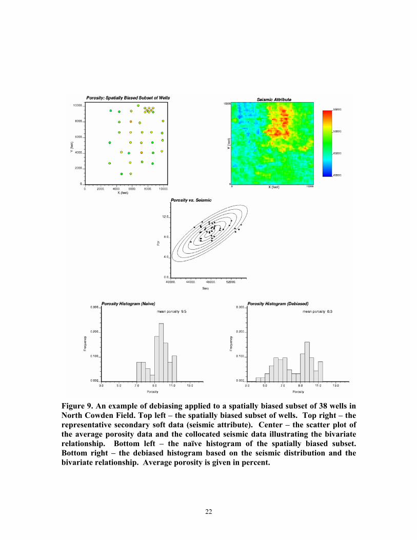
To illustrate the debiasing technique, a subset of 38 wells was chosen from the 62 wells in North Cowden Field such that the low porosity regions were not sampled (see the top left of Figure 9). Available seismic information was used as a representative data source to aid in inferring the entire porosity distribution (see top right of Figure 9). A potential bivariate relationship is indicated on the scatter plot of the porosity from the 38

9

spatially biased wells and the collocated seismic attribute (see center of Figure 9). The debiased porosity distribution is established by applying Equation 4. The original biased distribution and the resulting debiased distribution are shown on the bottom left and right of Figure 9, respectively.

Trend modeling and debiasing yield different results for integration into the full reservoir model. With trend modeling, the geostatistical simulation is augmented by information concerning the spatial behavior of the primary variable. Debiasing, on the other hand, relies on information concerning a more representative collection of secondary data and its relationship to the primary data. Data quality and sufficiency is key to the successful application of both methods, and the use of both methods has an impact on the uncertainty associated with the full reservoir model.

Parameters for Object Based Modeling Facies models constructed with object-based techniques reflect the well-defined

parametric shapes used as input. These shapes include channels, levees, crevasse splays, ellipsoidal concretions or remnant shales, barchan dunes, beach sand bars, submarine fans and so on. Provided the parametric shape is relevant to the reservoir, object based models are very appealing. Semivariogram-based facies models cannot represent shapes. However, they may be appropriate in settings where there are no clear shapes, as in the case of many carbonate reservoirs or diagenetically controlled facies.

The input shapes are often based on a conceptual geologic model and are not directly observed with reservoir data. There are notable exceptions where channel forms are sometimes observed in seismic reflections and wells intersect geologically well-defined rock types. Little can be done to validate the representativeness of estimates of model parameters such as these derived from a conceptual model. Therefore, it is important that the full range of shapes and sizes be considered.

The extent of various reservoir components must be evaluated in conjunction with the estimated shapes to arrive at unbiased size estimates. Consider the problem of inferring channel thickness from observed intersections in wells. Because the maximum channel thickness is the default value in most channel modeling software, and because channels are then determined on the basis of some postulated cross-section, the intersections in wells may be thinner than anticipated. They intersect the margin of an abandoned channel or the channel may have been eroded. Of course, the channels may also have amalgamated, leading to the possibility of choosing an erroneously large thickness. Consequently, all available information and expert judgment must be employed to estimate appropriate input distributions.

Analogue Data for the Semivariogram

The semivariogram and other spatial parameters are often difficult to estimate because the wells are too sparse or widely spaced. This does not detract from the importance of geostatistics. On the contrary, it makes the methodological choices even more important. Every numerical model has implicit (hidden from the modeler and

10

beyond their control) or explicit spatial statistical controls that must be taken into consideration.

A reliable horizontal semivariogram is particularly difficult to establish because the experimental horizontal semivariograms are often too noisy to interpret. However, the goal is to describe and represent the underlying phenomenon as accurately as possible, and not necessarily to obtain the best possible fit of the semivariogram. To do so, secondary information in the form of horizontal well data, seismic data, conceptual geological models, and analogue data must be considered; and expert judgment must be used to integrate global information from analogue data with sparse local data. In all cases, a systematic approach to the semivariogram interpretation is required (Gringarten and Deutsch, 2001).

In the absence of sufficient horizontal data, a horizontal semivariogram may be inferred by (1) determining the fraction of the variance that is explained by zonal anisotropy. (i.e., stratification that leads to persistent positive correlation in the horizontal direction), and then (2) establishing the horizontal-to-vertical anisotropy ratio based on secondary data. The inferred horizontal semivariogram consists of the zonal anisotropy (step one) and the scaled vertical semivariogram. Deutsch (2002) has published a table of typical anisotropy ratios that may aid in establishing the of horizontal-to-vertical anisotropy.

Figure 10 illustrates the relationship between these two types of anisotropy. Both the zonal anisotropy contribution and the horizontal-to-vertical anisotropy ratio have considerable uncertainty, which should be investigated via a sensitivity study and/or geostatistical simulation (Deutsch, 2002).

Size Scaling The input model parameters must also be consistent with the support size of the

model. Sample data are rarely, if ever, available at the support size of the model; therefore, the input values must be explicitly adjusted to reflect the support size prior to geostatistical simulation. Variances and semivariograms change with respect to well-understood scaling laws (Frykman and Deutsch, 2002). Figure 11 illustrates how a change in support size affects the histogram, variance, and semivariogram of porosity.

A change in the variance with respect to support size is characterized by a difference in semivariograms given by Equation 5.

),(),(),(2 vvVVVvD γγ −= , (5)

This equation states that the variance of volumes v within the larger volume V is the average point scale semivariogram within the larger volume minus the average point scale semivariogram within the smaller volume.

The required correction in variance is applied to the input histogram prior to geostatistical simulation by techniques such as affine and lognormal correction. The

11

nugget effect, variance contribution and range are corrected for change in support size, respectively, as follows:

||||

VvCC o

voV ⋅= , (6)

),(1),(1

vvVVCC i

viV γ

γ−−

= , (7)

|]||[| vVaa iv

iV −+= , (8)

In the above equations, the large V represents the block scale and the small v represents the data scale. For example, in Equation 6, |V| is the physical size in, say, cubic meters; and in Equation 8, |V| is the size of the domain in a particular direction. The range values in Equation 8 are different in different directions and they are affected by the original small-scale ranges as well as the geometry of the blocks under consideration.

Uncertainty in Hard and Soft Data

Log-derived facies and porosity values are interpretations of (error-prone) wireline measurements. Uncertainty thus derives from both the gathering and the interpretation process. More and more, practitioners are realizing that well data, generally considered “hard” in geostatistical simulation, have a certain degree of softness that must be considered in the modeling exercise. Similarly, secondary data sources (geological maps, seismically-derived attributes) that are considered as “soft” data limit stochastic simulation by removing a great deal of spatial variability from one realization to the next. It is important from a modeling point of view to account for variability in secondary data by considering multiple net-to-gross maps, multiple seismic attributes, or multiple representations of other such reservoir facets.

Uncertainty in the Input Parameters

Modern geostatistical reservoir modeling consists of generating realizations of all critical spatial parameters. The spatial parameters may include the top structure, the thickness, the facies, porosity, and permeability. These parameters are usually modeled hierarchically; for example, facies identification depends on structure, porosity depends on the identification of facies, and permeability depends on porosity. The number of realizations depends on the goals and the available computing and professional resources. Typically, 10 to 200 realizations are generated. A common approach is to produce a number of realizations independently and to avoid creating multiple facies models within a specified structural framework, or multiple porosity models for a given facies model, and so on. The resulting set of L realizations could be denoted

{topl(x,y), thkl(x,y), faciesl(x,y), porl(x,y,z), perml(x,y,z)}, l=1,…L, (9)

12

where x,y,z represent the areal and stratigraphic coordinates. Different deterministic and geostatistical simulation techniques may be used to construct the realizations (estimates) of each parameter. In addition, the realizations (estimates) generated for each parameter must encompass the range of possible input model parameters. For example, the net sand proportion may initially be set to 0.6; whereas it could very well fall between 0.5 and 0.7 because of limited well data. Nonetheless, while the different facies realizations may reflect a range of results, the practical difference between them is often quite small. As previously suggested, the ergodic fluctuations between realizations depends more on the size of the domain relative to the range of correlation than on the actual uncertainty in the parameter.

The operational flow of the simulation process proceeds as follows. An empirical or theoretical distribution is established for the estimates of each input model parameter, or an empirical histogram is produced. A value is selected at random from this distribution to be used in each realization. For example, the sand proportion could be modeled as a triangular distribution with a minimum of 0.5, a mode or 0.6, and a maximum of 0.7. A new target proportion would be drawn from this distribution for each realization. This basic idea, which is analogous to Monte Carlo simulation has been around for many years (Haldorsen and Damsleth, 1990) and is implemented in various software packages used for geostatistical modeling.

Note that the distribution of the estimates of each parameter must be established or postulated on the basis of concomitant information. Ideally, the choice derives from expert knowledge. For example, the project geologist chooses the range of object sizes, the geophysicist selects the range of correlation between acoustic impedance and porosity, the engineer determines the uncertainty in an interpreted well test k•h, and the geostatistician decides the minimum, most likely, and maximum semivariogram range. In the absence of expert knowledge, there are some quantitative tools to help establish the uncertainty in certain parameters. The bootstrap methodology (Efron, 1979) is one such approach.

The Bootstrap Approach

The bootstrap approach can be used in certain cases to assess the uncertainty in an input parameter. Given n data values from which a statistic s is calculated, additional sets of n data values are produced by sampling the original n values with replacement (e.g., using a Monte Carlo sampling process). The statistic s is calculated for each new set of n values, with the process being repeated a large number of times (on the order or 1000). The values of the statistic s computed for each of the new data sets are denoted s′ to distinguish them from the original value of s. The empirical distribution of s′is then used to approximate the unknown distribution of s. Efron(1979) discusses the reasonableness of using such an approximation.

Consider the cross-plot of vertical average porosity and seismic energy for the wells in North Cowden Field shown in Figure 12. The correlation coefficient is calculated to be 0.62. Being a sample statistic, this value has uncertainty associated with

13

it. Clearly the uncertainty would be greater if there were only 3 wells and the uncertainty would be less with more wells. The histogram on the right of Figure 12 is an empirical distribution of the correlation coefficient resulting from the bootstrap of pairs that can subsequently be carried through successive modeling steps.

An estimate of the correlation coefficient is simply selected at random from this distribution each time a geostatistical realization (estimate) of average porosity is produced.

There are two important assumptions implicit to the use of the bootstrap: (1) the data are independent, and (2) the data histogram is representative. The issue of data representativeness has been previously addressed and the steps proposed there should be undertaken prior to implementing the bootstrap procedure. The assumption of data independence is much more difficult to resolve. While wells in fields are often widely spaced making the independence assumption seem reasonable, core or well log data from within a single well is closely spaced, and the values of reservoir properties they represent certainly may not be independent.

Uncertainty in the Semivariogram

The semivariogram has a direct influence on the spatial arrangement of the petrophysical properties in a geostatistical reservoir model, but it does not directly affect the static resource. The level of model spatial variability, as modeled by the semivariogram, indirectly affects sweep efficiency and recovery. The semivariogram also affects the nature of ergodic fluctuations; For example, a larger range of correlation implies greater ergodic fluctuations. For these reasons, it is necessary to account for the uncertainty in the semivariogram and other spatial controls.

Uncertainty in the semivariogram may be assessed by expert judgment or by comparison to analogues representing similar depositional settings. The uncertainty in the semivariogram may also be estimated directly from the data as demonstrated by Ortiz and Deutsch (2002). For example, consider the experimental standardized normal score semivariogram of average porosity in the 62 North Cowden wells (Figure 13). The experimental semivariogram is very noisy due to limited data, and so the choice of a final model (curve) will not be very precise. To address this situation it is possible to construct a distribution of semivariogram ranges, as shown in Figure 13, so that for each realization, a semivariogram range is drawn at random from this distribution. This procedure transfers the uncertainty about the form of the semivariogram model (curve) to the full reservoir model.

Best Practices The following is the recommended workflow for the assembly of inputs to

stochastic models.

I. Review all data.

II. Assemble the most representative data.

14

III. Compute appropriate statistics with which to estimate all reservoir parameters.

IV. Quantify and incorporate the uncertainty associated with these statistics.

V. Generate realizations of the full reservoir model.

For the purpose of generating realizations of the full reservoir model that express the uncertainty in the input statistics, it is recommended that multiple realizations of each property be produced and that these realizations be linked as illustrated below and described in Equation 9. The important idea is that any realization of one reservoir property (e.g. porosity) may be dependent on the preceding realization of another (e.g., facies). Sensitivity analysis should be undertaken to evaluate the overall impact of each parameter. A sensitivity study can be performed by varying a single parameter (i.e., applying various estimates or realizations) while holding the others constant. This identifies key controlling parameters for which uncertainty in the input values must be refined to minimize uncertainty in the full reservoir model.

Summary The assembly of representative data is extraordinarily important to reservoir

modeling; the input statistics will be reproduced regardless of how representative they are of the underlying distributions; sound geological interpretation of major subsurface features and trends is a key step; they will not be reproduced “by chance” in the resulting geostatistical realizations. Interpretative and analogue information must be incorporated to ensure use of the most accurate and precise statistics, such as the histograms and semivariograms.

Uncertainty in the input statistics must be explicitly integrated into the full geostatistical reservoir model. Variation between realizations of this model is a function of the ratio of domain size to the range of correlation and not of the level of certainty in the input statistics. Uncertainty in the input statistics must be quantified by expert

Realization

Structure Facies Porosity Permeability

l=1 Structure1

Facies1 φ1 k1

l=2 Structure2

Facies2 φ2 k2

…

l=L Structuren

Faciesn φn kn

15

judgment, and where possible, by use of tools such as the bootstrap. This uncertainty may be imparted to the full reservoir model by varying the estimates of the model parameters according to their sampling distributions.

16

Bibliography

Deutsch, C.V., 2002, Geostatistical reservoir modeling: New York, Oxford University Press, 376 p.

Deutsch, C.V., and A.G. Journel, 1998, GSLIB - geostatistical software library and user’s guide: New York, Oxford University Press, 369 p.

Efron, B., 1979, Bootstrap methods: another look at the jackknife: The Annals of Statistics, v. 7, p. 1-26.

Frykman, P., and C.V. Deutsch, 1998, Model-based declustering for deriving representative distributions prior to conditional simulations: Second IMA Conference on Modelling Permeable Rocks, March 23-25, Churchill College, Cambridge.

Frykman, P., and C.V. Deutsch, 2002, Practical application of the geostatistical scaling laws for data integration: Petrophysics, v. 43, no. 3, p. 153-171.

Goovaerts, P., 1997, Geostatistics for natural resources evaluation: New York, Oxford University Press, 487 p.

Gringarten, E., and C.V. Deutsch, 2001, Variogram interpretation and modeling: Mathematical Geology, v. 33, no. 4, p. 507-534.

Haldorsen, H.H., and E. Damsleth, 1990, Stochastic modeling: Journal of Petroleum Technology, v. 42, p. 404-412.

Isaaks, E. H., and R.M. Srivastava, 1989, An introduction to applied geostatistics: New York, Oxford University Press, 561 p.

Ortiz C., J., and C.V. Deutsch, 2002, Calculation of the uncertainty in the variogram: Mathematical Geology, v. 34, no. 2, p. 169-183.

Vejbæk, O.V., and L. Kristensen, 2000, Downflank hydrocarbon potential identified using seismic inversion and geostatistics: Upper Maastrichtian reservoir unit, Dan Field, Danish Central Graben: Petroleum Geoscience, v. 6, p. 1-13.

17

Figure 1. The locations of all 62 wells in North Cowden Field, and four randomly selected wells (colored dots), along with the observed distribution of average vertical porosity (in percent) for all wells.

Figure 2. Three input distributions (low, base, and high cases) of average vertical porosity, two example realizations of a geostatistical model of average vertical porosity, generated with sequential Gaussian simulation conditioned to the four

18

sampled wells, based on each distribution, and, the resulting distributions of pore volume (million cubic feet assuming an average reservoir thickness of 10 feet) compiled from 101 realizations generated for each case.

Figure 3. The four sampled wells relative to three nested domains: Area 1, Area 2 and Area 3. The color bar indicates average vertical porosity.

19

Figure 4. The empirical distributions of average vertical porosity based on three realizations generated with sequential Gaussian simulation for each of the three domains. The distributions of the mean values from 101 realizations over each of the three domains are shown at the bottom.

20

Figure 5. An example horizontal and vertical trend calculated from all 62 wells. Average porosity is given in percent. Top - The trend in the horizontal may be calculated by a smooth fit of the vertically averaged data. Bottom - The vertical trend may be calculated using a smooth representation of porosity averaged over horizontal bins. Note the use of a stratigraphic z coordinate 0.0 to 1.0, indicating a proportional correlation style.

Figure 6. The effect of weighting data values. The data values remain the same but their relative weights are modified to account for spatial representativeness. Note the naïve histogram is slightly offset for visibility.

21

Figure 7. An example of cell declustering applied to the histogram of average porosity from a clustered subset of 37 wells in North Cowden Field. Top left - the clustered subset of wells with the Declustering cell size illustrated. Top right – the naïve, equally weighted, histogram. Bottom left – the declustered mean vs. cell size. Bottom right – the weighted histogram. Average porosity is given in percent.

Figure 8. An example of polygonal declustering applied to the histogram of average porosity from a clustered subset of 37 wells in North Cowden Field. Left – the polygons of influence used to assign data weights. Right – the weighted histogram. Average porosity is given in percent.

22

Figure 9. An example of debiasing applied to a spatially biased subset of 38 wells in North Cowden Field. Top left – the spatially biased subset of wells. Top right – the representative secondary soft data (seismic attribute). Center – the scatter plot of the average porosity data and the collocated seismic data illustrating the bivariate relationship. Bottom left – the naïve histogram of the spatially biased subset. Bottom right – the debiased histogram based on the seismic distribution and the bivariate relationship. Average porosity is given in percent.

23

Figure 10. A schematic illustration of the zonal anisotropy contribution and the horizontal-to-vertical anisotropy parameters required to infer a horizontal semivariogram in the absence of reliable horizontal experimental semivariograms (Deutsch, 2002).

24

Figure 11. An example of the effect of change in support size on the variance and the semivariogram. Note the decrease in variance and semivariogram sill and increase in semivariogram range with increase in support size. Porosity is given in percent.

25

Figure 12. An example of the bootstrap applied to the correlation coefficient between average porosity and a seismic attribute for all 62 wells in North Cowden Field. Left – the scatter plot between porosity and the seismic attribute. Right – the distribution of correlation coefficients from 1000 bootstrap iterations.

Figure 13. Uncertainty in the semivariogram. The experimental semivariogram (red dots) and three possible semivariogram models (curves) that encompass a possible distribution of the semivariogram range based on the experimental semivariogram.