Equi-RippleDesign ofQuadraticPhaseRFPulses

Rolf F. Schulte, Jeffrey Tsao, Peter Boesiger, and Klaas P. Pruessmann

Institute for Biomedical Engineering, University and Swiss Federal Institute of Technology Zurich, Gloriastr. 35, 8092 Zurich,Switzerland

Abstract

An improved strategy for the design of quadratic-phase RF pulses with high selectivity and broad bandwidths using the Shinnar-Le Roux (SLR) transformation is proposed. Unlike previous implementations, the required quadratic-phase finite impulseresponse (FIR) filters are generated using the complex Remez exchange algorithm, which ensures an equi-ripple deviation fromthe ideal response function. It is argued analytically that quadratic-phase pulses are near-optimal in terms of minimising theB1-amplitude for a given bandwidth and flip angle. Furthermore, several parameter relations are derived, providing practicaldesign guidelines. The effectiveness of the proposed design method is demonstrated by examples of excitation and saturationpulses applied in vitro and in vivo.

Key words: quadratic phase pulses, Shinnar-Le Roux transformation, broad bandwidth, very selective saturation pulses,frequency modulation

1 IntroductionMost magnetic resonance imaging (MRI) methods

rely on frequency selective radio-frequency (RF) pulses,which become spatially selective with the application ofmagnetic field gradients. The quality and usefulness ofsuch pulses is determined by several criteria, includingthe excitation profile, the maximum RF field strengthB1max, the deposited energy and the length of the pulse.The ideal slice profile is a rectangular function for highselectivity. In other words, the excitation should be uni-form within a chosen region and negligible outside thisregion. Furthermore, a broad excitation bandwidth isdesired to reduce problems like the chemical shift dis-placement or the sensitivity to B0 inhomogeneities.

In general, trade-offs have to be made among the var-ious criteria mentioned above in order to obtain prac-tically useful pulses. For common linear-phase pulses,which are essentially sinc-pulses, high selectivity requiresa long pulse duration with many side lobes. For a broadexcitation bandwidth, pulses of this type require highmaximum RF field strength B1max, which is ultimatelylimited by the RF amplifier. For example, a typical limitfor the B1 amplitude is about 10 µT on a whole-bodyMRI scanner. At this RF field strength, linear-phasepulses achieve about 1 kHz for a 90◦ flip angle and 500Hz for 180◦. However, much larger bandwidths are re-quired for many applications, especially at higher B0

field strengths. As shown in Ref. [1–3], overlaying RFpulses with a quadratic phase in the frequency domainresults in the RF energy of the main lobe being dis-

tributed more evenly over the pulse. Hence, for a givenB1max restriction, it is possible to achieve a broaderbandwidth and improved selectivity by using quadratic-phase pulses.

However, the quadratic phase of these pulses limitstheir application as general pulses, since they cannotbe refocused through linear gradients. Therefore, thesepulses are most useful for purposes that do not requirerefocusing, such as the saturation and inversion of mag-netisation. For these purposes, the phase distribution isirrelevant, while high selectivity, good agreement withthe target profile and broad bandwidth remain essen-tial. For instance, good outer volume suppression en-ables scanning with a reduced field of view and there-with reduced scan time in imaging [2]. Furthermore, thechemical shift displacement in PRESS can be reducedby saturating the region of displacement [4].

A straightforward way of obtaining pulses with anapproximately quadratic phase is to rescale adiabatic fullpassage pulses with offset independent adiabaticity [5].However, pulses with improved characteristics, such ashigher selectivity or error functions with constant errorripples, can be obtained by designing them from scratch.De novo design of RF pulses amounts to inverting theBloch equations. This is particularly convenient in thesmall-tip-angle approximation [6], where the RF waveform and the pulse response can be approximated bya Fourier pair. For the design of pulses with large flipangles, several methods of non-linear optimisation havebeen proposed, using for instance optimal control theory

Article published in Journal of Magnetic Resonance 166 (2004) 111-122.

[7,8] and simulated annealing [9].An elegant and more analytical approach is the

Shinnar-Le Roux (SLR) transformation [10,11], whichreversibly transforms RF pulses into two complex finiteimpulse response (FIR) filters. The frequency responseof these filters corresponds closely with the excitationprofile of the RF pulse. Hence, the problem of RF pulsedesign reduces to that of designing low pass FIR filters.In case of linear-phase filters, this is a standard proce-dure for which many methods exist. The SLR transformis frequently used to design linear-phase pulses, whichare purely amplitude-modulated. Nevertheless, the SLRconcept is equally applicable for the design of RF pulseswith frequency modulation, such as quadratic-phasepulses. However, FIR filters with a quadratic phase aremore intricate to design.

FIR filters are represented in the z-transform domainas finite-order polynomial functions of a complex vari-able (z). Quadratic phase requires complex polynomialcoefficients, which are generally more difficult to deter-mine than real-valued coefficients for linear-phase pulsesdue to increased algebraic complexity and possible ill-conditioning of the problem [12,13]. A simple solutionis to determine real and imaginary parts of the coef-ficients independently as though they were real-valuedcoefficients. This simplifies the problem, but does notgenerally yield the optimal solution [12].

Two methods have been previously proposed fordetermining the complex coefficients of approximatelyquadratic-phase FIR filters. The first one commences bydesigning a minimum-phase FIR filter with the desiredmagnitude response, whose phase pattern is then mod-ified by root inversion [14]. The maximum frequencybandwidth achievable with this method is small due tonumerical constraints and imprecise phase approxima-tions. The second method is to calculate the polynomialcoefficients of the desired FIR filter through a complexleast-squares algorithm [2]. This optimisation minimisesthe deviation from the ideal response in terms of the2-norm, which typically results in error overshoots atthe band edges. A more favourable solution is the equi-ripple solution, where all error ripples are minimisedto achieve equal magnitude. This is obtained by min-imising the ∞-norm (Chebyshev norm) of the errorfunction. An approximately equi-ripple error can also beobtained by introducing a proper weighting function inthe least-squares optimisation. The implementation ofthis approach, as described in [2], performs a weightedleast-squares fit to a pre-tailored target profile. Withthis method, the authors obtained an almost equi-ripplesolution with broad bandwidth and high selectivity.Nevertheless, they report restrictions to the range offeasible quadratic-phase patterns.

In this work, we propose to obtain the equi-ripplesolution directly, using the complex Remez exchangealgorithm [12,13]. This permits determining quadratic-phase pulses with a wide range of quadraticity fromzero (linear-phase) up to a critical maximum value. Inthe first part of the paper, the motivation for quadratic

phase is reviewed. A simple heuristic reasoning is fol-lowed by a mathematical argument, which illustratesthe near-optimality of quadratic phase pulses in termsof minimising B1max. Then several parameter relationsare described, providing design guidelines and illustrat-ing trade-offs among the various pulse properties. In thesubsequent sections, the actual design algorithms are de-scribed and validated by both simulations and MR ex-periments.

2 Motivation for Quadratic-Phase PulsesThe advantage of quadratic-phase pulses can be ap-

preciated by comparing them to linear-phase pulses.Most of the magnetisation in the selected band is rotatedsimultaneously with a linear-phase pulse. This requiresa short main lobe, as its width is inversely-proportionalto the bandwidth. The maximum B1-amplitude of suchpulses increases with the bandwidth, as the integralunderneath the main lobe remains approximately con-stant for a given flip angle. Therefore, the B1max andpower limitations of the transmit coil and the RF ampli-fier restrict the bandwidth achievable with linear-phasepulses.

The key idea for reducing RF peak power is to ex-cite the spins successively at their individual frequenciesrather than all at once [14]. By sweeping through the de-sired frequencies sequentially, the pulse energy does notneed to be confined to a single main lobe. Thus, the max-imum RF amplitude can be significantly reduced. Themost straightforward option, a linear frequency sweep,corresponds to multiplying the pulse envelope with aquadratic phase term. Interestingly, such a modulationalso results in an approximately quadratic phase pat-tern in the spectral response of the pulse. Thus, thequadratic-phase response forms a suitable design goalfor RF pulses with reduced peak power, enabling higherbandwidths. However, simply combining a linear fre-quency sweep with constant RF amplitude, forming aso-called chirp pulse, results in a poor excitation pro-file. Thus, more sophistication is needed to combine aquadratic phase response with a proper rectangular am-plitude profile.

The motivation for quadratic-phase pulses can alsobe argued from a more mathematical perspective, em-ploying the Fourier transformation (FT), which approx-imates the solution of the Bloch equation for pulses withsmall flip angles [6]. This approximation holds strictlyonly for pulses with small flip angles θ with sin θ ≈ θ,but it holds sufficiently well to qualitatively describe thebehaviour of pulses with a flip angle of up to about 90◦.

The ideal excitation profile |F (ω)| is rectangular

|F (ω)| = rect(ω), where

rect(ω) =

{0, for |ω| > BW/2,

sin θ, for |ω| ≤ BW/2,

(1)

where ω denotes the frequency, BW the bandwidth and

2

θ the flip angle. If F (ω) has a linear phase, the RF waveform f(t) = F (F (ω)) is a sinc-function with a sharppeak and a large number of significant side lobes. Here,F () denotes the Fourier transform. In contrast, for ef-ficient RF energy transfer in a limited time, the enve-lope f(t) should ideally be rectangular as well. That is,the pulse envelope should be approximately rectangularin both the time and the frequency domain. These twoseemingly conflicting requirements can be fulfilled onlywith a quadratic phase, as shown by Papoulis [15].

A rectangular function with an overlaid quadraticphase can be written as

f(t) =1√

−4πkirect

(t

2k

)e−

it24k , (2)

where k is a scaling constant and rect is defined as inEq. [1]. Eq. [2] is expressed in the frequency domain as

F (ω) =1√

−4πki· F

(rect

(t

2k

))⊗F

(e−

it24k

). (3)

The convolution in Eq. [3] can be developed into anasymptotic series, as shown in Ref. [15]. For a sufficientlylarge k and a sufficiently smooth envelope, this seriescan be approximated by

F (ω) ≈ eikω2rect(ω). (4)

In this expression, k specifies the amount of quadraticphase applied in the frequency domain. Generally, theFourier transform of a smooth envelope function with aquadratic phase yields the same envelope in the otherdomain, again with a quadratic phase. In the desiredrectangular profile, the smoothness criterion is violatedat the two discontinuities. As a consequence, the ideallyrectangular envelope in the time domain will deteriorateat its edges. Incidentally, by swapping t and ω, the samereasoning explains why chirp pulses, which have the idealrectangular profile in the time domain, have such poorexcitation profiles.

According to Parseval’s theorem

‖f(t)‖2 =

√√√√√ ∞∫−∞

|f(t)|2dt =‖F (ω)‖2

2π∝√

BW sin θ .(5)

Hence, the 2-norm is fixed for a given bandwidth BWand flip angle θ. In turn, for a fixed norm and pulseduration, the smallest peak amplitude is achieved bya pulse with a constant envelope (i.e., |f(t)| = const),which is accomplished precisely with quadratic phase inthe limit of large k. In other words, practical quadratic-phase pulses are almost optimal in terms of minimisingthe peak RF amplitude for a given pulse duration, band-width and flip angle.

Fig. 1. Effect of different amounts of quadratic phase k onthe magnitude of the RF pulse (Remez pulse with n = 512,θ = 90◦, ωp = 0.1π and ωs = 0.11π). The pulse at k = 0corresponds to a regular linear-phase pulse. For increasing kthe RF energy is spread out further and further away fromthe original central main lobe.

0 50 100 150 200 250 3000

0.05

0.1

0.15

0.2

0.25

0.3

0.35

0.4

0.45

0.5

(max(|B1|))2 k

(mean(|B1|))2 k

π /16

k

|B1|2 ⋅

k

Fig. 2. The square of the B1 amplitude of Fig. 1 times k isplotted against k, showing that Eq. [18] holds well in a widerange of k values. The dashed line denotes the maximum B1

value, the solid line is the mean value over the bandwidth cal-culated through Eq. [14] and the default value from Eq. [17]π16

with θ = π2

is plotted with a dash-dotted line.

3 Parameter Definitions and RelationsSuccessful design of quadratic-phase pulses that

match the target specifications closely requires trade-offs among the design parameters. The main parametersinclude the bandwidth

BW =ωs + ωp

2(6)

3

0 1 2 3 4 5

10−4

10−3

10−2

10−1

1

2 c

3

a

b

k ⋅ BW2 ⋅ FTW

Err

or

Complex Remez

0 1 2 3 4 5

10−4

10−3

10−2

10−1

1

2 c

3

a

b

k ⋅ BW2 ⋅ FTW

Err

or

Weighted Least Squares

Fig. 3. The pulse design error as a function of the parametersetting (varying k, BW , FTW ). The error plotted here isthe maximum error ripple, including the ripple in the tran-sition band exceeding the value of the pass band. In seriesa, b and c, the fractional transition width is held constant(FTW = 0.1) and the bandwidth is varied (a: BW ·n = 80.4,b: BW ·n = 160.8, c: BW ·n = 241.3). In the other series 1, 2and 3, the bandwidth is held constant (BW ·n = 241.3), whilethe fractional transition width is varied (1: FTW = 0.05,2: FTW = 0.1, 3: FTW = 0.125). Each series containsthree lines, corresponding to three different filter lengths(n = 256, n = 512, n = 1024). Beyond a critical value ofk · BW 2 · FTW ≈ 3.6 (vertical line), the pulse design errorincreases sharply due to the emergence of an overshoot inthe transition band.

−3 −2 −1 0 1 2 30

0.2

0.4

0.6

0.8

1

ω

|Mxy

|

Fig. 4. Unfavourable parameter selection (i.e., too high(k BW 2 FTW ) product) can lead to high overshoots insidethe transition band. As this band is not considered duringthe fitting procedure, one has to choose a different parame-ter set. Here: k BW 2 FTW = 14.

and the fractional transition width

FTW =ωs − ωp

BW, (7)

which is a relative expression for the selectivity. ωs andωp are the stop and pass band frequencies. Further keyparameters are the flip angle θ, the filter length n andthe amount of quadratic phase k. The parameter settings

lead to certain pulse properties, such as the maximumRF amplitude B1max, the energy of the pulse and theresulting error function, which is defined as the devia-tion from the target profile. In the following, several re-lationships among pulse parameters and properties areestablished as design guidelines.

To clarify the subsequent description, it is importantto distinguish between normalised and physical quan-tities. In FIR filter design, the frequency ω is usuallynormalised to the range [−π, π]. The inverse SLR trans-formation can be used to convert such filters into anRF pulse shape with normalised time, whose duration isequal to the filter length n. This pulse can then be scaledto any physical duration, thus rescaling frequency andtime to physical units. Throughout this paper, physicalfrequency and time will be distinguished from their nor-malised counterparts by the tilde symbol. The quantitiesin physical units are given by:

ω̃ =ω

∆t̃, (8)

T̃ = n∆t̃, (9)

k̃ = k∆t̃2, (10)

B̃1 =B1

γ∆t̃, (11)

where ∆t̃ denotes the sample spacing, T̃ the total du-ration of the pulse and γ the gyromagnetic ratio. Withthese relationships it is straightforward to scale an RFpulse to different pulse durations.3.1 Time-Bandwidth Product

The physical bandwidth of the RF pulse is given by

˜BW =BW

∆t̃. (12)

With Eq. [9] this leads to the time-bandwidth productof the RF pulse

T̃ ˜BW = n BW, (13)

which is invariant under time and frequency scaling andthus is a key characteristic of an RF pulse. This productis fundamentally limited by digitisation. For quadratic-phase pulses, an estimate of this limitation can be de-rived from Eqs. [2] and [4] for moderate flip angles. Ide-ally, the cutoff values of the rectangular functions in thetwo domains are related through ω = t

2k , leading to

BW =n

2k. (14)

As mentioned, when enforcing a good rectangular shapein the frequency domain, the corresponding profile in thetime domain will degrade at its edges and extend beyond

4

the idealised pulse duration. In order to still capture theentire pulse, Eq. [14] must allow for some slack in thetime domain. This results in

BW � n

2k. (15)

Combined with Eq. [13], this yields

T̃ ˜BW � n2

2k. (16)

That is, for achieving a high time-bandwidth productwith a given k value, n must be sufficiently large. Notethat k needs to be large as well in order to justify theseries expansion underlying Eq. [4] and to reduce B1max,as discussed in the following.3.2 Amount of Quadratic Phase

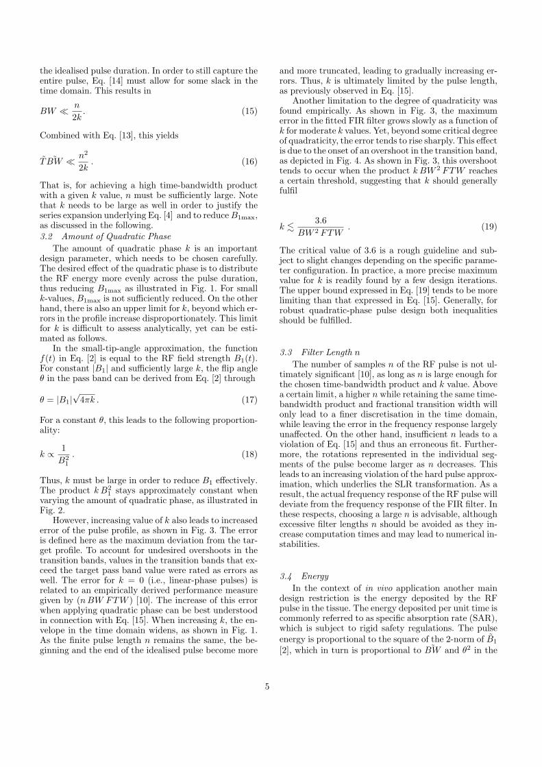
The amount of quadratic phase k is an importantdesign parameter, which needs to be chosen carefully.The desired effect of the quadratic phase is to distributethe RF energy more evenly across the pulse duration,thus reducing B1max as illustrated in Fig. 1. For smallk-values, B1max is not sufficiently reduced. On the otherhand, there is also an upper limit for k, beyond which er-rors in the profile increase disproportionately. This limitfor k is difficult to assess analytically, yet can be esti-mated as follows.

In the small-tip-angle approximation, the functionf(t) in Eq. [2] is equal to the RF field strength B1(t).For constant |B1| and sufficiently large k, the flip angleθ in the pass band can be derived from Eq. [2] through

θ = |B1|√

4πk . (17)

For a constant θ, this leads to the following proportion-ality:

k ∝ 1B2

1

. (18)

Thus, k must be large in order to reduce B1 effectively.The product k B2

1 stays approximately constant whenvarying the amount of quadratic phase, as illustrated inFig. 2.

However, increasing value of k also leads to increasederror of the pulse profile, as shown in Fig. 3. The erroris defined here as the maximum deviation from the tar-get profile. To account for undesired overshoots in thetransition bands, values in the transition bands that ex-ceed the target pass band value were rated as errors aswell. The error for k = 0 (i.e., linear-phase pulses) isrelated to an empirically derived performance measuregiven by (n BW FTW ) [10]. The increase of this errorwhen applying quadratic phase can be best understoodin connection with Eq. [15]. When increasing k, the en-velope in the time domain widens, as shown in Fig. 1.As the finite pulse length n remains the same, the be-ginning and the end of the idealised pulse become more

and more truncated, leading to gradually increasing er-rors. Thus, k is ultimately limited by the pulse length,as previously observed in Eq. [15].

Another limitation to the degree of quadraticity wasfound empirically. As shown in Fig. 3, the maximumerror in the fitted FIR filter grows slowly as a function ofk for moderate k values. Yet, beyond some critical degreeof quadraticity, the error tends to rise sharply. This effectis due to the onset of an overshoot in the transition band,as depicted in Fig. 4. As shown in Fig. 3, this overshoottends to occur when the product k BW 2 FTW reachesa certain threshold, suggesting that k should generallyfulfil

k .3.6

BW 2 FTW. (19)

The critical value of 3.6 is a rough guideline and sub-ject to slight changes depending on the specific parame-ter configuration. In practice, a more precise maximumvalue for k is readily found by a few design iterations.The upper bound expressed in Eq. [19] tends to be morelimiting than that expressed in Eq. [15]. Generally, forrobust quadratic-phase pulse design both inequalitiesshould be fulfilled.

3.3 Filter Length n

The number of samples n of the RF pulse is not ul-timately significant [10], as long as n is large enough forthe chosen time-bandwidth product and k value. Abovea certain limit, a higher n while retaining the same time-bandwidth product and fractional transition width willonly lead to a finer discretisation in the time domain,while leaving the error in the frequency response largelyunaffected. On the other hand, insufficient n leads to aviolation of Eq. [15] and thus an erroneous fit. Further-more, the rotations represented in the individual seg-ments of the pulse become larger as n decreases. Thisleads to an increasing violation of the hard pulse approx-imation, which underlies the SLR transformation. As aresult, the actual frequency response of the RF pulse willdeviate from the frequency response of the FIR filter. Inthese respects, choosing a large n is advisable, althoughexcessive filter lengths n should be avoided as they in-crease computation times and may lead to numerical in-stabilities.

3.4 EnergyIn the context of in vivo application another main

design restriction is the energy deposited by the RFpulse in the tissue. The energy deposited per unit time iscommonly referred to as specific absorption rate (SAR),which is subject to rigid safety regulations. The pulseenergy is proportional to the square of the 2-norm of B̃1

[2], which in turn is proportional to ˜BW and θ2 in the

5

Amplitude

|Mxy(ω)|

Phase

∠ Mxy(ω)

Amplitude

|A(ω)|

|B(ω)|

Phase

∠ A(ω)

∠ B(ω)

Amplitude modulation

Phase modulation

Amplitude

A|B|

Phase

∠ B

Bloch Equation

RF Pulse A/B Polynomials

Klein

z Transform

SLR

Cayley−

Freq

. Dom

ain

Tim

e D

omai

n

3 4

1 2

Fig. 5. The relationships between the different domains as-sociated with the Shinnar-Le Roux (SLR) transform, shownfor a typical quadratic-phase RF pulse. The SLR transformlinks the RF pulse (1) with an equivalent pair of FIR fil-ters, A and B. The coefficient (2) and frequency (4) repre-sentations of these filters are connected by the z-transform.The frequency response of the FIR filters is related to theexcitation profile of the RF pulse (3) by the Cayley-Kleinrotational parameters. The excitation profile can equally beobtained by directly integrating the Bloch equations (1 ⇒3). However, in the reverse direction the direct pathway,i.e., Bloch inversion, is generally not available. Instead, SLRpulse design operates via the stages 4 and 2, exploiting thereversibility of the intermediate transforms.

small-tip-angle regime (Eq. [5])

Q ∝T̃ /2∫

−T̃ /2

|B̃1(t̃)|2dt̃ ∝ ˜BW θ2. (20)

Frequency modulation can be neglected here, as it is farlower than the precession frequency.

For low flip angles, the pulse energy Q depends solelyon the flip angle and the bandwidth ˜BW as derivedin Eq. [20]. Thus, pulses with the same bandwidth andflip angle deposit the same energy [2]. In other words,quadratic-phase pulses behave like regular linear-phasepulses in this respect, at least in the small-tip-angleregime.

4 MethodsThe SLR transformation converts the problem of in-

verting the Bloch equations into that of designing twocomplex polynomials A(z) and B(z), which representregular FIR filters. Hence, it is possible to use the com-prehensive methodology of FIR filter design for RF pulsedesign. A(z) and B(z) are (n − 1)th order polynomi-als that represent the frequency-dependent Cayley-Kleinparameters of the rotation effected by the correspond-ing RF pulse. For instance, the transverse magnetisationcreated by a pulse from initial z-magnetisation of M0 isgiven by [10]

Mxy = 2A(z)∗B(z)M0, (21)

such that

End

2 steps

s ωE )||(||

s ωE )||(||Construct a new subset

increasesS

s ωE )||(||

S of > n+1 points− Subset

S withimation on a subset

No

an optimal norm

Compute the best approx−

EndYes

S

End

No

Yeschanged?

= ||E (ω)|| ?

2 steps

− SubsetSof n+1 pointsComplex Remez:

Multiple Exchange Ascent:

Stage 2

Step 2

Stage 1Step 1

Fig. 6. Schematic of the algorithm for finding the optimal FIRfilter B(ω). The solution is characterised by a minimum ofthe Chebyshev norm of the error function E(ω), correspond-ing to equi-ripple error. Two stages (left) iterate through atwo-step process until the optimal solution is found. The sec-ond stage is invoked only if the first stage fails to converge.

where the asterisk denotes complex conjugation and z =eiω is the argument of the polynomials. In the following,“A(z)” and “B(z)” will be used interchangeably with“A(ω)” and “B(ω)” for notational convenience. Sincethe Cayley-Klein polynomials represent rotations, theysatisfy the following constraint

A(z)A∗(z) + B(z)B∗(z) = 1, (22)

for all values of z, which leads to

|Mxy(ω)| = 2√

1− |B(ω)|2 · |B(ω)|M0 . (23)

Hence, if |B(ω)| describes a rectangular profile as a func-tion of ω, the excited transverse magnetisation |Mxy(ω)|will also exhibit a rectangular envelope. For the designof low pass pulses, it is thus possible to first design asuitable B polynomial and then generate a matchingA polynomial that satisfies Eq. [22]. Typically, and inthe current work as well, the A polynomial is createdthrough the Hilbert transform, leading to a minimum-phase frequency response of A, as described in Ref. [10].When the phase of A is negligible, the phase of Mxy willbe similar to that of the B polynomial. Therefore, an RFpulse with a quadratic-phase frequency response can begenerated on the basis of a B FIR filter with a quadraticphase and a corresponding minimum-phase A polyno-mial. The relationship between the RF pulse and the Aand B polynomials is depicted in Fig. 5.

In the following, two methods are described for cre-ating FIR filters with complex coefficients. The firstmethod is least-squares optimisation, which employs aweighting function for obtaining an approximately equi-

6

ripple error function, as previously suggested in Ref. [2].The second one is the proposed method, which uses thecomplex Remez exchange algorithm [12,13] to directlyachieve a truly equi-ripple error function without theneed for heuristic spectral weighting. This algorithm is ageneralisation of the Remez/Parks-McClellan algorithm[16], which permits approximating arbitrary magnitudeand phase response functions.4.1 Target Filter Response

The desired frequency response, to which B(ω) willbe fitted, is expressed as

D(ω) = R(ω)eiϕ(ω), (24)

where R(ω) and ϕ(ω) are real-valued functions, describ-ing the desired magnitude and phase responses, respec-tively. For a low pass quadratic-phase response, they areexpressed as:

R(ω) =

{0, for |ω| ≥ ωs,

sin(

θ2

), for |ω| ≤ ωp,

ϕ(ω) = kω2, (25)

where θ is the desired flip angle and ωp and ωs are thepass and stop band frequencies. The gaps between thepass and the stop bands are referred to as the transitionbands. The sin (θ/2) originates from the SLR transfor-mation and is derived from Eq. [23] by setting |Mxy| to(M0 sin θ) for 0 ≤ θ ≤ π. It should be noted, that ω isthe symmetric and normalised frequency in the range[−π, π]. In the literature, the range of ω is frequently de-fined as [0, 2π] with a centre frequency of π. This onlyrefers to a shift of reference, and in that case ϕ(ω) wouldinclude a linear phase term as well. Note also, that it iseasily possible to extend this target to an asymmetricfunction, for instance to obtain one sharper side.4.2 Error Function

The FIR filter to be designed is a polynomial of theform

B(ω) =n−1∑j=0

bje−ijω , (26)

where bj denotes the complex jth polynomial coefficient.The difference between this filter and the desired re-sponse function D(ω) is expressed by the error function

E(ω) = W (ω) (D(ω)−B(ω)) , (27)

where W (ω) is a real and non-negative weighting func-tion. In the transitions bands, W (ω) is generally set tozero.4.3 Least-Squares Fit

As described in [2], a least-squares fit of the targetfilter response is obtained by minimising the 2-norm of

the error function

‖E(ω)‖2 =

√√√√√ π∫−π

|E(ω)|2dω . (28)

With uniform error weighting this approach leads toovershoots at the band edges. However, the weightingfunction W (ω) can be adjusted to place more empha-sis in these areas and thus reduce overshoots. A feasibleweighting function for an approximately equi-ripple so-lution was found to be [2]

W (ω) =

1

δ(ω)

√√√√1 + 10

(1(

ω − 12(ωs + ωp)

)2 +1(

ω + 12(ωs + ωp)

)2)

,

(29)

where δ(ω) = δ1 is the relative target ripple of thepolynomial in the pass band, δ(ω) = δ2 in the stop bandand δ(ω) = ∞ (i.e., W (ω) = 0) in the transition band.

For numerical treatment, the normalised frequencyω must be discretised. An equi-distant discretisation ofthe frequency is given by

ωl = ∆ω

(l +

12

)− π , (30)

where ∆ω = 2π/m denotes the sampling frequency andthe index l counts from 0 to (m − 1). The number ofsampling points m needs to be much larger than thefilter length n for sufficient accuracy.

Using this discretisation, the minimisation problemcan be reformulated in terms of matrix notation. Theactual and desired filter responses B and D, and the er-ror function E are transformed into the vectors B,D,Eby sampling along ωl. By assembling the polynomial co-efficients bj from Eq. [26] in a similar fashion, the actualfilter response can be expressed as

B = Ub , (31)

where the entries of the m× n matrix U are given by

ul,j = e−ijωl . (32)

The weighting function from Eq. [29] can be incorpo-rated as an m×m diagonal matrix W, with its diagonalelements given by

wl,l = W (ωl) . (33)

Hence, Eq. [27] can be restated as

E = W (D−Ub) , (34)

7

and the optimal coefficient vector b is characterised bya minimum of the 2-norm of E. The minimum-normsolution can be calculated with the Moore-Penrose [17]pseudo-inverse (†)

b = (WU)†WD . (35)

4.4 Complex Remez for Chebyshev-NormIn the proposed method, the truly equi-ripple solu-

tion is obtained by finding filter coefficients that min-imise the Chebyshev (i.e., maximum) error norm

‖E(ω)‖∞ = maxω{|E(ω)|}, (36)

with E(ω) defined as in Eq. [27]. The major advan-tage of Chebyshev optimisation is that it does not re-quire a particular weighting function for approximatingequi-ripple behaviour. It minimises the maximum error,which forces the magnitudes of the error ripples to bethe same everywhere. Therefore, the weighting functionW (ω) is now constant everywhere apart from the transi-tion bands, which are exempt from optimisation. Never-theless, one may also choose to apply different constantweights on the pass and stop bands in order to individ-ually alter the magnitude of the error ripples in the dif-ferent bands.

Chebyshev optimisation of FIR filters with complexcoefficients can be accomplished with the complex Re-mez exchange algorithm. For a detailed description of thealgorithm, the reader is referred to Refs. [12,13]. Briefly,to minimise the Chebyshev norm efficiently, the mainstrategy is to sample E(ω) only at a sparse, finite subsetS of frequencies and iteratively adapt these frequenciessuch that they sample the extreme values of the errorripples. This basic approach consists of two steps, whichare depicted on the right in Fig. 6. In a first step, the bestapproximation in terms of ‖ES(ω)‖∞ (Eq. [36]) on thesparse subset is calculated. In a second step, this subsetis altered such that the maximum error norm ‖ES(ω)‖∞of this subset increases. The optimal solution is founditeratively repeating both steps until the subsets remainthe same.

The complex Remez algorithm (Fig. 6, top left) per-forms these steps with subsets of n + 1 points, where nis the filter length. In this case, the minimisation prob-lem on each subset reduces to a linear system of equa-tions, which can be solved very efficiently. The optimalsolution is found when the error norm on the subset,‖ES(ω)‖∞, converges toward the actual error norm onthe continuous set, ‖E(ω)‖∞. This is generally the casefor parameter sets that comply with the relations de-scribed in Sect. 3. For the case of non-convergence of thecomplex Remez algorithm, a more advanced method wasdescribed in [13]. This method, a generalised multiple-exchange ascent algorithm, forms the optional secondstage of the optimisation procedure (Fig. 6, bottom left).It performs the same steps as described above, yet sam-ples the error function more densely and uses a more

intricate method for subset iteration. Using the resultof the first stage as an initial estimate, the second stageconverges safely, yet at the expense of drastically in-creased computation time. However, it was found em-pirically that the second algorithm needs to be invokedonly in cases with unfavourable parameter relations. Inthese cases, even the optimal solution must typically bediscarded due to high error levels. For the present work,the complex Remez and multiple-exchange ascent al-gorithms were performed under MATLAB (The Math-Works, Inc., Natick, MA, USA), using an implementa-tion available in the signal processing toolbox.

4.5 Validation StudyTo validate the proposed methods, an exemplary RF

pulse was designed with a time-bandwidth product of330 (in radians), a fractional transition width of 0.073, aflip angle of θ = 90◦, k = 120, and n = 512 samples. Forcomparison, two pulses with the same specifications wereadditionally designed using the least-squares approachwith either the weighting function given by Eq. [29] orconstant weights.

The excitation profiles of these pulses were verifiedby numerical integration of the Bloch equations employ-ing a fourth-order Runge-Kutta method [18]. Addition-ally, the pulses were verified experimentally on a Philips1.5 T Intera whole-body MR scanner equipped witha transmit/receive birdcage resonator (Philips MedicalSystems, Best, The Netherlands). Both excitation andsaturation capabilities were shown on a phantom con-taining one litre of doped water solution (T1 = 360ms; T2 = 320 ms). Furthermore, the saturation of mag-netisation was demonstrated in vivo in an axial sectionthrough the human brain. Written informed consent wasobtained from the healthy volunteer prior to imaging.

All experiments were based on regular spin echoimaging sequences. In the excitation experiments, thequadratic-phase RF pulse was used for 90◦ excitation,with a selection gradient in the same direction as thereadout gradient. The 180◦ refocusing pulse was thenused to select the image plane (TE = 40 ms, TR = 800ms). In the saturation experiments, the quadratic-phasepulse was used for exciting the magnetisation, again ina perpendicular slice, followed by spoiler gradients andthe full spin-echo sequence with normal slice selection(TE = 30 ms, TR = 800 ms).

5 ResultsThe amplitude and frequency modulation of the ex-

emplary pulse (see Sect. 4.5) is shown in Fig. 7. Fora duration of T̃ = 5 ms it has a maximum RF fieldstrength of B̃1max = 20µT. For comparison, the maxi-mum RF field strength of a linear-phase pulse with thesame specifications is more than three-fold at B̃1max =68µT. The complex Remez design is compared to thealternative design methods in Fig. 8. The upper rowshows the magnitude of the deviation between the de-sired and the achieved profiles designed with the complexRemez, weighted least-squares and plain least-squares

8

100 200 300 400 5000

0.02

0.04

0.06Amplitude modulation

|B1|

100 200 300 400 500−5

0

5x 10

4 Frequency modulation

Time

d∠ B

1/dt

Fig. 7. Quadratic-phase pulse designed with the complexRemez exchange algorithm. The design parameters were:n = 512, θ = 90◦, ωp = 0.095π, ωs = 0.11π and k = 120.This pulse was used for the validation study (Figs. 11 and12).

10−4

10−2

100

B(ω

) E

rror

Least Squares

10−8

10−6

10−4

10−2

100

Mxy

Err

or

−pi/2 0 pi/2 pi

10−8

10−6

10−4

10−2

100

Mz E

rror

ω

Weighted Least Squares

−pi/2 0 pi/2 pi

ω

Complex Remez

−pi/2 0 pi/2 pi

ω

Fig. 8. Comparison of FIR filter design with least-squares(left), weighted-least-squares (middle), and complex Remez(right), based on the pulse specifications given in Fig. 7.The top row shows the error in the FIR filter response|B(ω)−D(ω)|. The structure of the error ripples is illustratedin the magnified insets. The two major peaks in each plotcorrespond to the transition bands and do not represent ac-tual errors. Only the complex Remez algorithm yields errorripples of constant magnitude throughout the pass and stopbands. The middle and bottom rows show the resulting er-ror in the transverse and longitudinal magnetisation, respec-tively. For the magnetisation the error levels differ betweenthe pass and stop bands, reflecting the non-linear relation-ship between B(ω) and the components of the magnetisation(Eq. [23]).

−pi −pi/2 0 pi/2 pi10

−10

10−8

10−6

10−4

10−2

100

ω

Mxy

Err

or

Complex Remez

−pi −pi/2 0 pi/2 pi10

−10

10−8

10−6

10−4

10−2

100

ω

Mz E

rror

Complex Remez

Fig. 9. Error in the transverse (∣∣|Mxy| − |M ideal

xy |∣∣ ; left)

and longitudinal (∣∣Mz −M ideal

z

∣∣ ; right) magnetisations, ob-tained with a quadratic-phase complex Remez pulse. Thepulse specifications were the same as for Figs. 7 and 8. How-ever, different error weighting was applied in the pass andstop bands to match the ripple magnitude in all three bands.For equi-ripple transverse magnetisation (left), the weighton the stop bands was exaggerated 140-fold. For equi-ripplelongitudinal magnetisation (right), the weight on the passband was exaggerated 300-fold.

−3 −2 −1 0 1 2 3

0

0.2

0.4

0.6

0.8

1

−50%

−30%

0%+30%

+50%

ω

|Mxy

|

−3 −2 −1 0 1 2 3

−0.6

−0.4

−0.2

0

0.2

0.4

0.6

0.8

1

−50%

−30%

−10%

0%

+10%

+30%

+50%

ω

Mz

Fig. 10. Pulse profiles of quadratic-phase pulses generallydeteriorate as B̃1 is simply scaled to different flip angles. 0%denotes the original B̃1 for a flip angle of 90◦. Scaling the RFfield by the indicated percentage alters the pulse profile asshown. For high profile quality, quadratic-phase pulses mustbe designed specifically for the target flip angle.

0

0.5

1

|Mxy

|

10

20

30

40

∠ M

xy [r

ad]

0

0.2

0.4

0.6

0.8

1

|Mz|

Fig. 11. Excitation (Mxy, left) and saturation (Mz, right)profiles obtained with a quadratic-phase Remez pulse, assimulated with a Runge-Kutta method (dashed) and mea-sured experimentally using a water phantom (solid). In thesaturation profile (right) a region outside of the phantom isincluded, reflecting the noise level present in the data set.

algorithms. These results illustrate that direct Cheby-shev optimisation yields an exact equi-ripple error func-tion, while some variation in the error level is obtainedwith either weighted or plain least-squares.

From the A and B polynomials, the transverse mag-netisation was calculated through Mxy = 2A∗BM0 andthe longitudinal magnetisation through Mz = (AA∗ −BB∗)M0 [10], setting M0 to one. In the middle and

9

Sig

nal [

a.u.

]

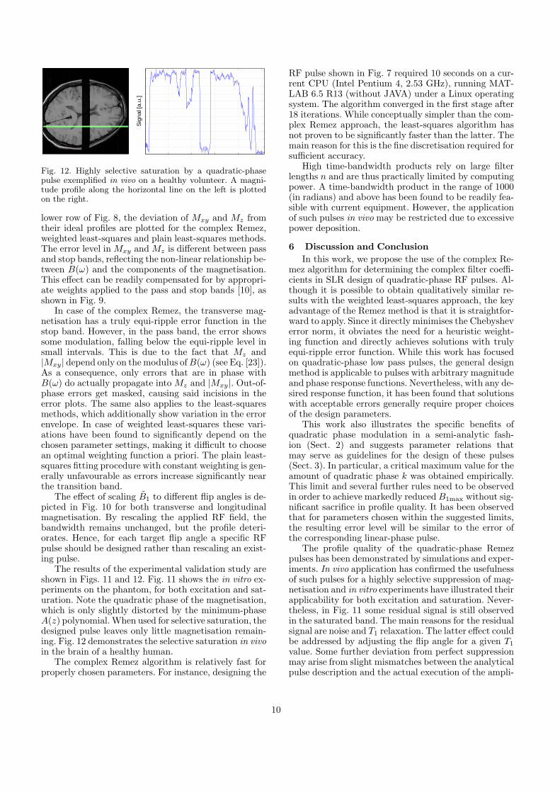
Fig. 12. Highly selective saturation by a quadratic-phasepulse exemplified in vivo on a healthy volunteer. A magni-tude profile along the horizontal line on the left is plottedon the right.

lower row of Fig. 8, the deviation of Mxy and Mz fromtheir ideal profiles are plotted for the complex Remez,weighted least-squares and plain least-squares methods.The error level in Mxy and Mz is different between passand stop bands, reflecting the non-linear relationship be-tween B(ω) and the components of the magnetisation.This effect can be readily compensated for by appropri-ate weights applied to the pass and stop bands [10], asshown in Fig. 9.

In case of the complex Remez, the transverse mag-netisation has a truly equi-ripple error function in thestop band. However, in the pass band, the error showssome modulation, falling below the equi-ripple level insmall intervals. This is due to the fact that Mz and|Mxy| depend only on the modulus of B(ω) (see Eq. [23]).As a consequence, only errors that are in phase withB(ω) do actually propagate into Mz and |Mxy|. Out-of-phase errors get masked, causing said incisions in theerror plots. The same also applies to the least-squaresmethods, which additionally show variation in the errorenvelope. In case of weighted least-squares these vari-ations have been found to significantly depend on thechosen parameter settings, making it difficult to choosean optimal weighting function a priori. The plain least-squares fitting procedure with constant weighting is gen-erally unfavourable as errors increase significantly nearthe transition band.

The effect of scaling B̃1 to different flip angles is de-picted in Fig. 10 for both transverse and longitudinalmagnetisation. By rescaling the applied RF field, thebandwidth remains unchanged, but the profile deteri-orates. Hence, for each target flip angle a specific RFpulse should be designed rather than rescaling an exist-ing pulse.

The results of the experimental validation study areshown in Figs. 11 and 12. Fig. 11 shows the in vitro ex-periments on the phantom, for both excitation and sat-uration. Note the quadratic phase of the magnetisation,which is only slightly distorted by the minimum-phaseA(z) polynomial. When used for selective saturation, thedesigned pulse leaves only little magnetisation remain-ing. Fig. 12 demonstrates the selective saturation in vivoin the brain of a healthy human.

The complex Remez algorithm is relatively fast forproperly chosen parameters. For instance, designing the

RF pulse shown in Fig. 7 required 10 seconds on a cur-rent CPU (Intel Pentium 4, 2.53 GHz), running MAT-LAB 6.5 R13 (without JAVA) under a Linux operatingsystem. The algorithm converged in the first stage after18 iterations. While conceptually simpler than the com-plex Remez approach, the least-squares algorithm hasnot proven to be significantly faster than the latter. Themain reason for this is the fine discretisation required forsufficient accuracy.

High time-bandwidth products rely on large filterlengths n and are thus practically limited by computingpower. A time-bandwidth product in the range of 1000(in radians) and above has been found to be readily fea-sible with current equipment. However, the applicationof such pulses in vivo may be restricted due to excessivepower deposition.

6 Discussion and ConclusionIn this work, we propose the use of the complex Re-

mez algorithm for determining the complex filter coeffi-cients in SLR design of quadratic-phase RF pulses. Al-though it is possible to obtain qualitatively similar re-sults with the weighted least-squares approach, the keyadvantage of the Remez method is that it is straightfor-ward to apply. Since it directly minimises the Chebysheverror norm, it obviates the need for a heuristic weight-ing function and directly achieves solutions with trulyequi-ripple error function. While this work has focusedon quadratic-phase low pass pulses, the general designmethod is applicable to pulses with arbitrary magnitudeand phase response functions. Nevertheless, with any de-sired response function, it has been found that solutionswith acceptable errors generally require proper choicesof the design parameters.

This work also illustrates the specific benefits ofquadratic phase modulation in a semi-analytic fash-ion (Sect. 2) and suggests parameter relations thatmay serve as guidelines for the design of these pulses(Sect. 3). In particular, a critical maximum value for theamount of quadratic phase k was obtained empirically.This limit and several further rules need to be observedin order to achieve markedly reduced B1max without sig-nificant sacrifice in profile quality. It has been observedthat for parameters chosen within the suggested limits,the resulting error level will be similar to the error ofthe corresponding linear-phase pulse.

The profile quality of the quadratic-phase Remezpulses has been demonstrated by simulations and exper-iments. In vivo application has confirmed the usefulnessof such pulses for a highly selective suppression of mag-netisation and in vitro experiments have illustrated theirapplicability for both excitation and saturation. Never-theless, in Fig. 11 some residual signal is still observedin the saturated band. The main reasons for the residualsignal are noise and T1 relaxation. The latter effect couldbe addressed by adjusting the flip angle for a given T1

value. Some further deviation from perfect suppressionmay arise from slight mismatches between the analyticalpulse description and the actual execution of the ampli-

10

tude and frequency modulations by the MR system.Numerous applications may benefit from the

quadratic-phase pulses, which exhibit large bandwidthand high selectivity. Reduced field-of-view imaging andnon-echo volume selection in spectroscopy are two appli-cations already mentioned. Another prime applicationis the inversion of magnetisation. Currently, this taskis often performed with adiabatic pulses. However, twofactors favour the use of specifically designed quadraticphase pulses: for given time and B1max restrictions bet-ter profiles can be achieved and the pulse energy willgenerally be lower than for adiabatic pulses. Such pulseswill find use in many inversion-prepared sequences, inparticular arterial spin labelling, where high selectivityis crucial.

While less intuitive, quadratic phase RF pulses mayindeed also be used for selective excitation, e.g., in 3Dimaging [19,20]. Here, the additional phase encoding andFourier reconstruction along the selection direction canmake the quadratic phase variation negligible at thevoxel scale. For common 2D imaging, quadratic phasemodulation across a selected slice is usually a problembecause it cannot be unwound with linear external gra-dients. Alternatively, phase compensation can be doneby consecutive pulses with quadratic phase, where eachpulse cancels the phase of the previous one [21]. Anotherway is to combine multiple pulse segments into a com-posite pulse [22], as originally done to create an adiabaticspin-echo pulse [23]. The downsides of these approachesare higher power deposition and longer pulse duration.

Finally, non-linear through-plane modulation may aswell be exploited as a beneficial effect. Examples for suchapplications are spatial encoding by quadratic phase[24] and various methods for compensating B0 inhomo-geneity by quadratic- and tailored-phase RF pulses [25–27]. Requiring RF pulses with specific target phase re-sponses, these methods will benefit from the flexibilityand accuracy of complex Remez design.

7 AcknowledgementsThe authors would like to thank Andreas Trabesinger

for reviewing the manuscript. This work was supportedby Philips Medical Systems (Best, NL); Eureka; KTI(grant numbers E!2061; 4178.1), INCA-MRI. JeffreyTsao is a recipient of a postdoctoral fellowship from theCanadian Institutes of Health Research (CIHR).

References[1] D. W. Kunz, Use of frequency-modulated radiofrequency

pulses in MR imaging experiments, Magn Reson Med 3 (3)(1986) 377–384.

[2] P. Le Roux, R. J. Gilles, G. C. McKinnon, P. G. Carlier,Optimized outer volume suppression for single-shot fast spin-echo cardiac imaging, J Magn Reson Imaging 8 (5) (1998)1022–1032.

[3] D. W. Kunz, H. H. Tuithof, J. H. M. Cuppen, Method anddevice for determining an NMR distribution in a region of abody, United States Patent 4,707,659 (1987).

[4] T. K. C. Tran, D. B. Vigneron, N. Sailasuta, J. Tropp, P. LeRoux, J. Kurhanewicz, S. Nelson, R. Hurd, Very selective

suppression pulses for clinical MRSI studies of brain andprostate cancer, Magn Reson Med 43 (1) (2000) 23–33.

[5] Y. Luo, R. A. de Graaf, L. DelaBarre, A. Tannus,M. Garwood, BISTRO: An outer-volume suppression methodthat tolerates RF field inhomogeneity, Magn Reson Med45 (6) (2001) 1095–1102.

[6] J. M. Pauly, D. G. Nishimura, A. Macovski, A k-spaceanalysis of small-tip-angle excitation, J Magn Reson 81 (1)(1989) 43–56.

[7] S. M. Conolly, D. G. Nishimura, A. Macovski, Optimalcontrol solutions to the magnetic resonance selectiveexcitation problem, IEEE T Med Imaging MI-5 (2) (1986)106–115.

[8] J. Mao, T. H. Mareci, K. N. Scott, E. R. Andrew, Selectiveinversion radiofrequency pulses by optimal control, J MagnReson 70 (2) (1986) 310–318.

[9] H. Geen, S. Wimperis, R. Freeman, Band-selective pulseswithout phase distortion. A simulated annealing approach, JMagn Reson 85 (3) (1989) 620–627.

[10] J. M. Pauly, P. Le Roux, D. G. Nishimura, A. Macovski,Parameter relations for the Shinnar-Le Roux selectiveexcitation pulse design algorithm, IEEE T Med Imaging10 (1) (1991) 53–65.

[11] M. Shinnar, J. S. Leigh, The application of spinors to pulsesynthesis and analysis, Magn Reson Med 12 (1) (1989) 93–98.

[12] L. J. Karam, J. H. McClellan, Complex Chebyshevapproximation for FIR filter design, IEEE T Circuits-II 42 (3)(1995) 207–216.

[13] L. J. Karam, J. H. McClellan, Chebyshev digital FIR filterdesign, Signal Process 76 (1) (1999) 17–36.

[14] M. Shinnar, Reduced power selective excitation radiofrequency pulses, Magn Reson Med 32 (5) (1994) 658–660.

[15] A. Papoulis, Signal Analysis, Chapter 8, McGraw-Hill, 1977.

[16] T. W. Parks, J. H. McClellan, Chebyshev approximation fornonrecusrive digital filters with linear phase, IEEE TransCircuit Theory CT 19 (2) (1972) 189–194.

[17] G. H. Golub, C. F. van Loan, Matrix Computations, 3rdEdition, The Johns Hopkins University Press, 1996, Ch. 5.

[18] K. P. Pruessmann, M. A. Spiegel, G. R. Crelier, M. Stuber,M. B. Scheidegger, P. Boesiger, Fast simulation of MR-excitation considering flow and motion, in: Proc Intl Soc MagReson Med 5, 1997, p. 1537.

[19] J. M. Pauly, E. C. Wong, Non-linear phase RF pulses forreduced dynamic range in 3D RARE imaging, in: Proc IntlSoc Mag Reson Med. 9, 2001, p. 688.

[20] L. DelaBarre, P. J. Bolan, M. Garwood, Improving dynamicrange in 3D MRI with RF pulses producing quadratic phase,in: Proc Intl Soc Mag Reson Med 9, 2001, p. 690.

[21] D. W. Kunz, Frequency-modulated radiofrequency pulses inspin-echo and stimulated-echo experiments, Magn Reson Med4 (2) (1987) 129–136.

[22] K. E. Cano, M. A. Smith, A. J. Shaka, Adjustable,broadband, selective excitation with uniform phase, J MagnReson 155 (1) (2002) 131–139.

[23] S. M. Conolly, D. G. Nishimura, A. Macovski, A selectiveadiabatic spin-echo pulse, J Magn Reson 83 (2) (1989) 324–334.

[24] J. G. Pipe, Spatial encoding and reconstruction in MRI withquadratic phase profiles, Magn Reson Med 33 (1) (1995) 24–33.

11

[25] Z. H. Cho, Y. M. Ro, Reduction of susceptibility artifact ingradient-echo imaging, Magn Reson Med 23 (1) (1992) 193–200.

[26] N. Chen, A. M. Wyrwicz, Removal of intravoxel dephasingartifact in gradient-echo images using a field-map based RFrefocusing technique, Magn Reson Med 42 (4) (1999) 807–812.

[27] A. W. Song, Single-shot EPI with signal recovery from thesusceptibility-induced losses, Magn Reson Med 46 (2) (2001)407–411.

12