reproducibility of complex turbulent flow using ... · reproducibility of complex turbulent flow...

Reports of Research Institute for Applied Mechanics, Kyushu University No.150 (47–59) March 2016

Reproducibility of Complex Turbulent Flow Using Commercially-Available CFD Software

―Report 1: For the Case of a Three-Dimensional Isolated-Hill With Steep Slopes―

Takanori UCHIDA*1

E-mail of corresponding author: [email protected]

(Received January 29, 2016)

Abstract

Selecting a high-quality site for wind turbine installation is frequently challenging in Japan because the majority of the topography of Japan is steep complex terrain and the spatial distribution of the wind speed is quite complex over such terrain. To address this issue, an unsteady CFD model called RIAM-COMPACT® has been developed. RIAM-COMPACT® is based on an LES turbulence model. In the present paper, to assess the accuracy of RIAM-COMPACT®, we performed a numerical simulation of uniform, non-stratified airflow past a three-dimensional isolated-hill. Attention is focused on airflow characteristics in the wake region. The results of RIAM-COMPACT® using the LES model were in good agreement with those of another commercially-available CFD software (STAR-CCM+) using LES models. Key words: Commercially-available CFD software, STAR-CCM+, RIAM-COMPACT®, LES, RANS, Isolated-hill

1．Introduction

The author’s research group has developed the numerical

wind synopsis prediction technique named RIAM-

COMPACT®1,

2). The core technology of RIAM-

COMPACT® is under continuous development at the

Research Institute for Applied Mechanics, Kyushu University.

An exclusive license of the core technology has been granted

by Kyushu TLO Co., Ltd. (Kyushu University TLO) to

RIAM-COMPACT Co., Ltd. (http://www.riam-compact.

com/), a venture corporation which was founded by the

author and originated at Kyushu University in 2006. A

trademark, RIAM-COMPACT®, and a utility model patent

were granted to RIAM-COMPACT Co., Ltd. in the same

year. In the meantime, a software package has been

developed based on the above-mentioned technique and is

named the RIAM-COMPACT® natural terrain version

software. Efforts have been made to promote this software as

a standard model in the wind power industry.

Some of the major corporations, which have adopted the

RIAM-COMPACT® software, are Eurus Energy Holdings

Corporation, Electric Power Development Co., Ltd.

(J-POWER), Japan Wind Development Co., Ltd., and

EcoPower Co., Ltd. etc.

Computation time had been an issue of concern for the

RIAM-COMPACT® software, which focuses on unsteady

turbulence simulations (LES, Large-Eddy Simulation). The

present fluid simulation solver is compatible with multi-core

CPUs (Central Processing Units) such as the Intel Core i7

and also with GPGPU (General Purpose computing on GPU),

which has drastically reduced the computation time, leaving

no appreciable problems in terms of the practical use of the

RIAM-COMPACT® software.

In the present study, simulation results of airflow over an

isolated-hill with steep slopes obtained from the RIAM-

COMPACT® software are compared to those from another

commercially-available CFD (Computational Fluid

Dynamics) software. The results from this comparison are

reported.

2. Summary of Commercially-Available CFD Software

Commercially-available CFD software has developed

mainly as an engineering tool primarily in the automobile and

aviation industries until the present time. The following is a

list of the major CFD software packages available on the

market:

General-purpose CFD thermal fluid analysis software

■STAR-CCM+

http://www.cd-adapco.co.jp/products/star_ccm_plus/index.

html ■ANSYS (CFD, Fluent, CFX)

http://ansys.jp/solutions/analysis/fluid/index.html ■SCRYU/Tetra

http://www.cradle.co.jp/products/scryutetra/

*1 Research Institute for Applied Mechanics, Kyushu University

48 Uchida : Reproducibility of Complex Turbulent Flow Using Commercially-Available CFD Software, Report 1

■STREAM

http://www.cradle.co.jp/products/stream/index.html ■CFD2000

http://www.cae-sc.jp/docs/cfd2000/index.htm ■PHOENICS

http://www.phoenics.co.jp/ ■Autodesk Simulation CFD

http://www.cfdesign.com/ ■CFD++

http://bakuhatsu.jp/software/cfd/ ■CFD-ACE+

http://www.wavefront.co.jp/CAE/cfd-ace-plus/ ■AcuSolve

http://acusolve.jsol.co.jp/index.html ■FLOW-3D

http://www.terrabyte.co.jp/FLOW-3D/flow3d.htm ■FloEFD

http://www.sbd.jp/product/netsu/floefd3cad.shtml ■Flow Designer

http://www.akl.co.jp/ ■PowerFLOW

http://www.exajapan.jp/pages/products/pflow_main.html ■KeyFlow

http://www.kagiken.co.jp/product/keyflow/index.shtml ■OpenFOAM

http://www.cae-sc.jp/docs/FOAM/ ■FrontFlow

http://www.advancesoft.jp/product/advance_frontflow_red/

The wind power industry has on its own developed and

distributed CFD software designed for selecting sites

appropriate for the installation of wind power generators (see

the listing below). Recently, some of the above-mentioned

general-purpose thermal fluid analysis software has started

being adopted in the wind power industry.

CFD software designed for the wind power industry (wind

farm design tools) ■RIAM-COMPACT®

http://www.riam-compact.com/ ■MASCOT

http://aquanet21.ddo.jp/mascot/ ■WindSim

http://www.windsim.com/

■METEODYN

http://meteodyn.com/

In the present study, the simulation results from the

RIAM-COMPACT® software are compared to those from

STAR-CCM+, one of the leading commercially-available

CFD software packages. The results of the comparison are

discussed.

3. Summary of STAR-CCM+ Software

In this section, a summary of STAR-CCM+, a general-

purpose thermal fluid analysis software package distributed

by CD-adapco will be provided. The version of the software

package used in the present study is 6.02.007 (for 64-bit

Windows).

STAR-CCM+ uses a single GUI (Graphical User

Interface) for computational mesh generation, execution of

fluid analyses, and data post-processing. In the present study,

a three-dimensional model of an isolated-hill (IGES format)

is created using CATIA, a three-dimensional CAD software

package developed by Dassault Systèmes. After reading in

the created three-dimensional CAD data on STAR-CCM+,

the mesh type, the mesh spacing, the turbulence model

(details to be described later), the time-step interval, the

boundary conditions, and other variables are set.

Subsequently, pre-processing, fluid analyses, and

post-processing are performed.

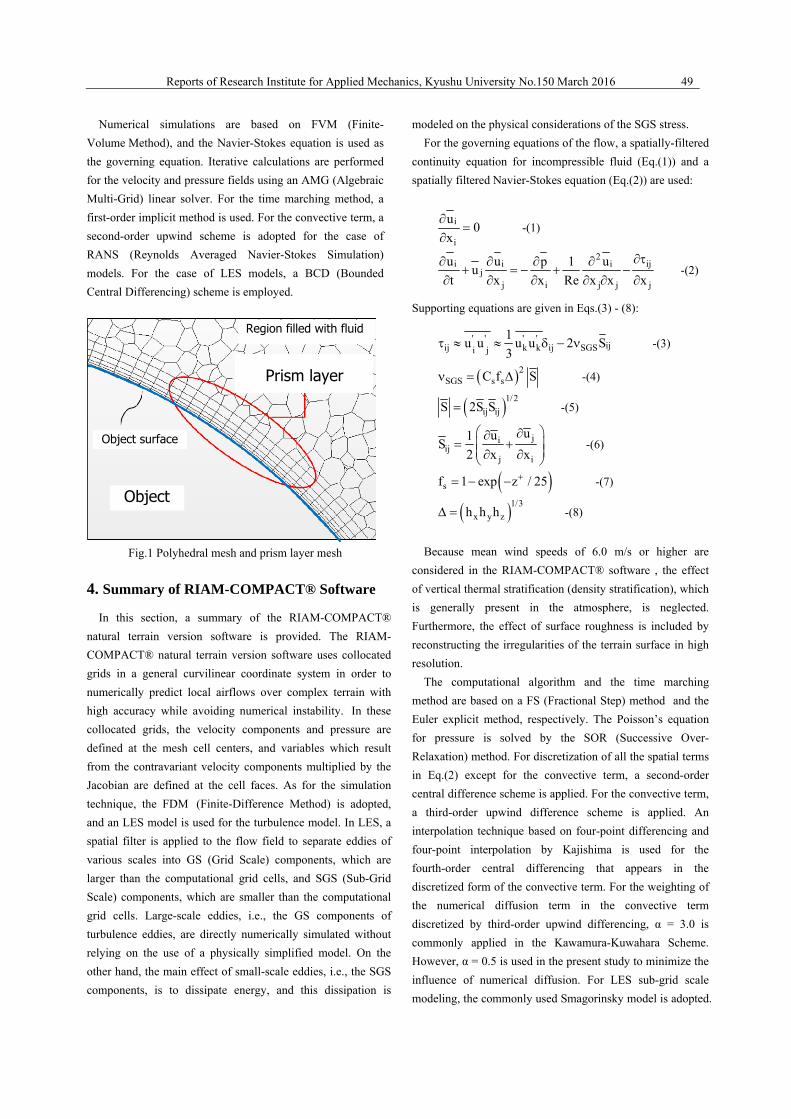
The mesh generation method in STAR-CCM+ is

distinctive. In STAR-CCM+, both a polyhedral mesh and a

prism layer mesh can be used (see Fig.1). The polyhedral

mesh is a new type of mesh offered by CD-adapco and

consists of polyhedral cells which possess 10 to 15 faces on

average. The use of this cell type makes it possible to

dramatically reduce the number of mesh cells required to

obtain analysis results equivalent to those that can be

obtained using a conventional tetrahedral mesh and 2) the

memory required by the solver. With the use of this cell type,

the computational stability improves significantly, and the

time required to obtain convergent solutions also decreases.

The prism layer mesh is a refined mesh designed to capture

the behavior of the boundary layer developed over an object.

In this type of mesh, layers of thin mesh cells are distributed

regularly over the object. Since the thickness and the number

of layers in the normal direction with respect to the object

surface can be freely adjusted, the behavior of the boundary

layer in the vicinity of a wall can be captured with high

accuracy. However, when the number of the prism layer

mesh cells is very large, the computation time increases

significantly.

Reports of Research Institute for Applied Mechanics, Kyushu University No.150 March 2016 49

Numerical simulations are based on FVM (Finite-

Volume Method), and the Navier-Stokes equation is used as

the governing equation. Iterative calculations are performed

for the velocity and pressure fields using an AMG (Algebraic

Multi-Grid) linear solver. For the time marching method, a

first-order implicit method is used. For the convective term, a

second-order upwind scheme is adopted for the case of

RANS (Reynolds Averaged Navier-Stokes Simulation)

models. For the case of LES models, a BCD (Bounded

Central Differencing) scheme is employed.

Fig.1 Polyhedral mesh and prism layer mesh

4. Summary of RIAM-COMPACT® Software

In this section, a summary of the RIAM-COMPACT®

natural terrain version software is provided. The RIAM-

COMPACT® natural terrain version software uses collocated

grids in a general curvilinear coordinate system in order to

numerically predict local airflows over complex terrain with

high accuracy while avoiding numerical instability. In these

collocated grids, the velocity components and pressure are

defined at the mesh cell centers, and variables which result

from the contravariant velocity components multiplied by the

Jacobian are defined at the cell faces. As for the simulation

technique, the FDM (Finite-Difference Method) is adopted,

and an LES model is used for the turbulence model. In LES, a

spatial filter is applied to the flow field to separate eddies of

various scales into GS (Grid Scale) components, which are

larger than the computational grid cells, and SGS (Sub-Grid

Scale) components, which are smaller than the computational

grid cells. Large-scale eddies, i.e., the GS components of

turbulence eddies, are directly numerically simulated without

relying on the use of a physically simplified model. On the

other hand, the main effect of small-scale eddies, i.e., the SGS

components, is to dissipate energy, and this dissipation is

modeled on the physical considerations of the SGS stress.

For the governing equations of the flow, a spatially-filtered

continuity equation for incompressible fluid (Eq.(1)) and a

spatially filtered Navier-Stokes equation (Eq.(2)) are used:

i

i

u0

x

-(1)

2iji i i

jj i j j j

u u p 1 uu

t x x Re x x x

-(2)

Supporting equations are given in Eqs.(3) - (8):

' ' ' 'ijij k k ij SGSi j

1u u u u 2 S

3 -(3)

2SGS s sC f S -(4)

1/2

ij ijS 2S S -(5)

jiij

j i

uu1S

2 x x

-(6)

sf 1 exp z / 25 -(7)

1/3

x y zh h h -(8)

Because mean wind speeds of 6.0 m/s or higher are

considered in the RIAM-COMPACT® software , the effect

of vertical thermal stratification (density stratification), which

is generally present in the atmosphere, is neglected.

Furthermore, the effect of surface roughness is included by

reconstructing the irregularities of the terrain surface in high

resolution.

The computational algorithm and the time marching

method are based on a FS (Fractional Step) method and the

Euler explicit method, respectively. The Poisson’s equation

for pressure is solved by the SOR (Successive Over-

Relaxation) method. For discretization of all the spatial terms

in Eq.(2) except for the convective term, a second-order

central difference scheme is applied. For the convective term,

a third-order upwind difference scheme is applied. An

interpolation technique based on four-point differencing and

four-point interpolation by Kajishima is used for the

fourth-order central differencing that appears in the

discretized form of the convective term. For the weighting of

the numerical diffusion term in the convective term

discretized by third-order upwind differencing, α = 3.0 is

commonly applied in the Kawamura-Kuwahara Scheme.

However, α = 0.5 is used in the present study to minimize the

influence of numerical diffusion. For LES sub-grid scale

modeling, the commonly used Smagorinsky model is adopted.

Region filled with fluid

Object surface

Object

Prism layer


A wall-damping function is used with a model coefficient of

0.1.

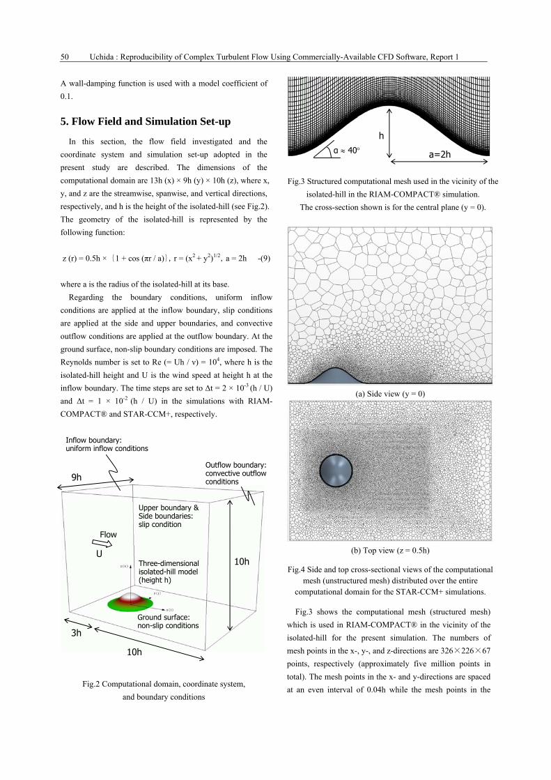
5. Flow Field and Simulation Set-up

In this section, the flow field investigated and the

coordinate system and simulation set-up adopted in the

present study are described. The dimensions of the

computational domain are 13h (x) × 9h (y) × 10h (z), where x,

y, and z are the streamwise, spanwise, and vertical directions,

respectively, and h is the height of the isolated-hill (see Fig.2).

The geometry of the isolated-hill is represented by the

following function:

z (r) = 0.5h × ｛1 + cos (πr / a)｝，r = (x2 + y2)1/2，a = 2h -(9)

where a is the radius of the isolated-hill at its base.

Regarding the boundary conditions, uniform inflow

conditions are applied at the inflow boundary, slip conditions

are applied at the side and upper boundaries, and convective

outflow conditions are applied at the outflow boundary. At the

ground surface, non-slip boundary conditions are imposed. The

Reynolds number is set to Re (= Uh / ν) = 104, where h is the

isolated-hill height and U is the wind speed at height h at the

inflow boundary. The time steps are set to Δt = 2 × 10-3 (h / U)

and Δt = 1 × 10-2 (h / U) in the simulations with RIAM-

COMPACT® and STAR-CCM+, respectively.

Fig.2 Computational domain, coordinate system,

and boundary conditions

Fig.3 Structured computational mesh used in the vicinity of the

isolated-hill in the RIAM-COMPACT® simulation.

The cross-section shown is for the central plane (y = 0).

(a) Side view (y = 0)

(b) Top view (z = 0.5h)

Fig.4 Side and top cross-sectional views of the computational mesh (unstructured mesh) distributed over the entire

computational domain for the STAR-CCM+ simulations.

Fig.3 shows the computational mesh (structured mesh)

which is used in RIAM-COMPACT® in the vicinity of the

isolated-hill for the present simulation. The numbers of

mesh points in the x-, y-, and z-directions are 326×226×67

points, respectively (approximately five million points in

total). The mesh points in the x- and y-directions are spaced

at an even interval of 0.04h while the mesh points in the

10h

9h

10h 3h

Flow

U

Ground surface: non-slip conditions

Three-dimensional isolated-hill model (height h)

Outflow boundary:convective outflow conditions

Upper boundary & Side boundaries: slip condition

Inflow boundary: uniform inflow conditions

h

a=2h α 40


z-direction are spaced unevenly (from 0.003h to 0.6h).

Fig.4 shows the computational mesh (unstructured mesh)

used in the present STAR-CCM+ simulations. The total

number of mesh points is approximately one million (i.e.,

approximately 1/5 of that used in the RIAM-COMPACT®

simulation). In the STAR-CCM+ simulations, the mesh

resolution in the vicinity of the isolated-hill is set to be

nearly identical to that in the RIAM-COMPACT®

simulation.

Tables 1 and 2 summarize all of the turbulence models

(RANS, LES) adopted in the present comparative study. For

convenience, simulations performed with the use of each of

the models are referred to as Cases 1 to 5. In Case 4, i.e., the

WALE model, the eddy viscosity coefficient becomes zero

near the wall without the use of a wall damping function.

Furthermore, this model has been designed in such a way

that the eddy viscosity coefficient is not calculated for

laminar shear layers.

Case 1

Spalart-Allmaras single equation

eddy-viscosity turbulence model,

steady RANS RANS

models

Case 2

SST k-ω two-equation eddy

-viscosity model, unsteady RANS

(URANS)

Case 3 Smagorinsky model, LES LES

models Case 4 WALE model, LES

Table 1 Turbulence models used in the present

STAR-CCM+ simulations

LES model Case 5 Smagorinsky model, LES

Table 2 Turbulence model used in the present

RIAM-COMPACT® simulation

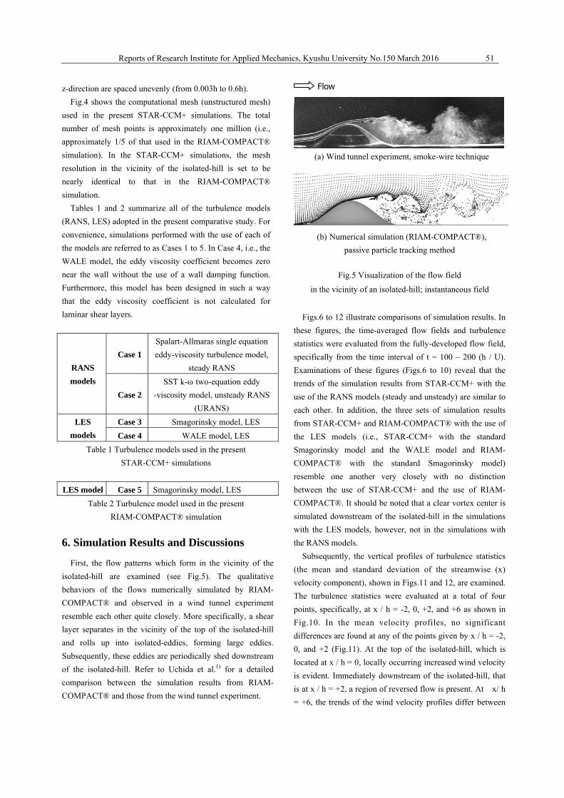
6. Simulation Results and Discussions

First, the flow patterns which form in the vicinity of the

isolated-hill are examined (see Fig.5). The qualitative

behaviors of the flows numerically simulated by RIAM-

COMPACT® and observed in a wind tunnel experiment

resemble each other quite closely. More specifically, a shear

layer separates in the vicinity of the top of the isolated-hill

and rolls up into isolated-eddies, forming large eddies.

Subsequently, these eddies are periodically shed downstream

of the isolated-hill. Refer to Uchida et al.1) for a detailed

comparison between the simulation results from RIAM-

COMPACT® and those from the wind tunnel experiment.

(a) Wind tunnel experiment, smoke-wire technique

(b) Numerical simulation (RIAM-COMPACT®),

passive particle tracking method

Fig.5 Visualization of the flow field

in the vicinity of an isolated-hill; instantaneous field

Figs.6 to 12 illustrate comparisons of simulation results. In

these figures, the time-averaged flow fields and turbulence

statistics were evaluated from the fully-developed flow field,

specifically from the time interval of t = 100 – 200 (h / U).

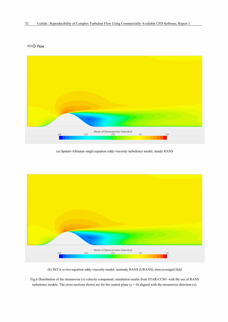
Examinations of these figures (Figs.6 to 10) reveal that the

trends of the simulation results from STAR-CCM+ with the

use of the RANS models (steady and unsteady) are similar to

each other. In addition, the three sets of simulation results

from STAR-CCM+ and RIAM-COMPACT® with the use of

the LES models (i.e., STAR-CCM+ with the standard

Smagorinsky model and the WALE model and RIAM-

COMPACT® with the standard Smagorinsky model)

resemble one another very closely with no distinction

between the use of STAR-CCM+ and the use of RIAM-

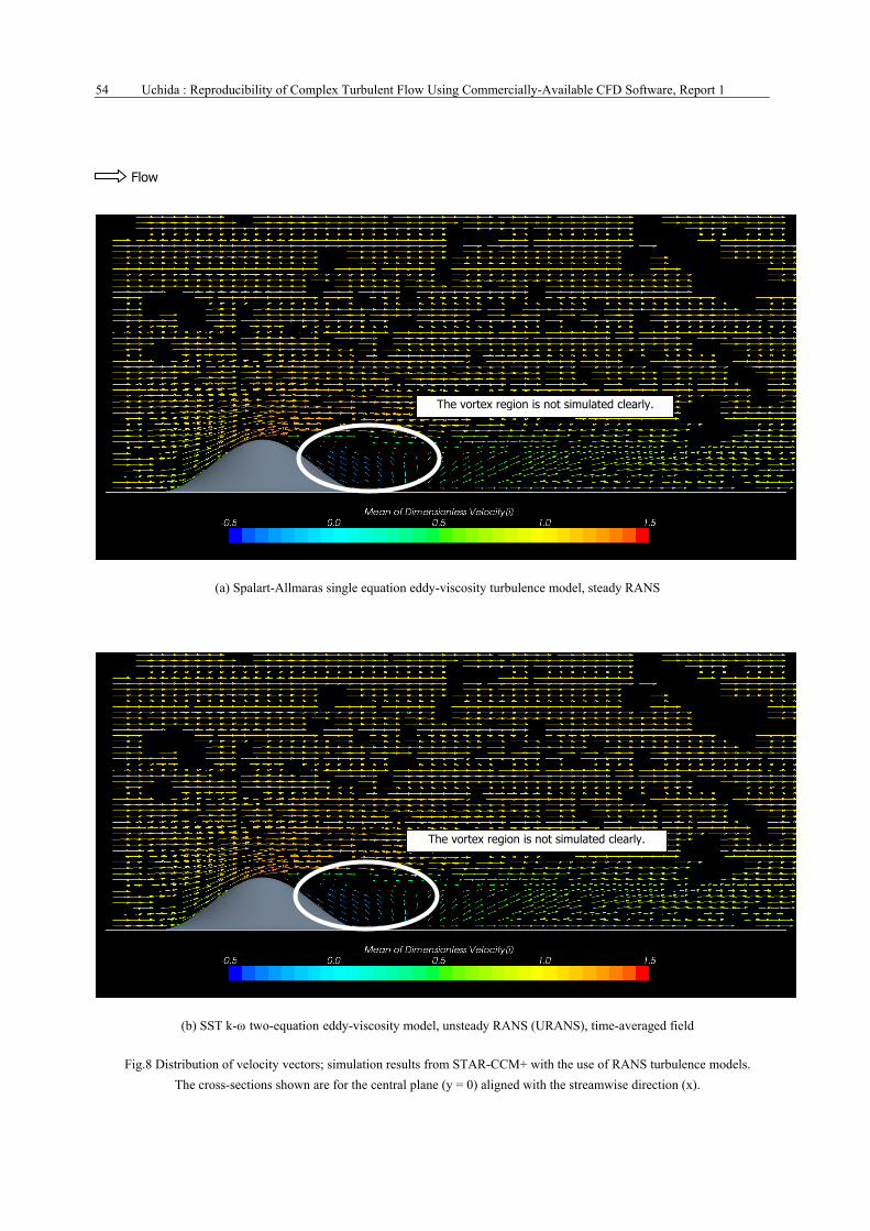
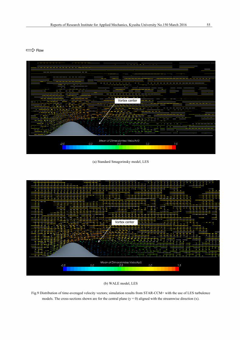
COMPACT®. It should be noted that a clear vortex center is

simulated downstream of the isolated-hill in the simulations

with the LES models, however, not in the simulations with

the RANS models.

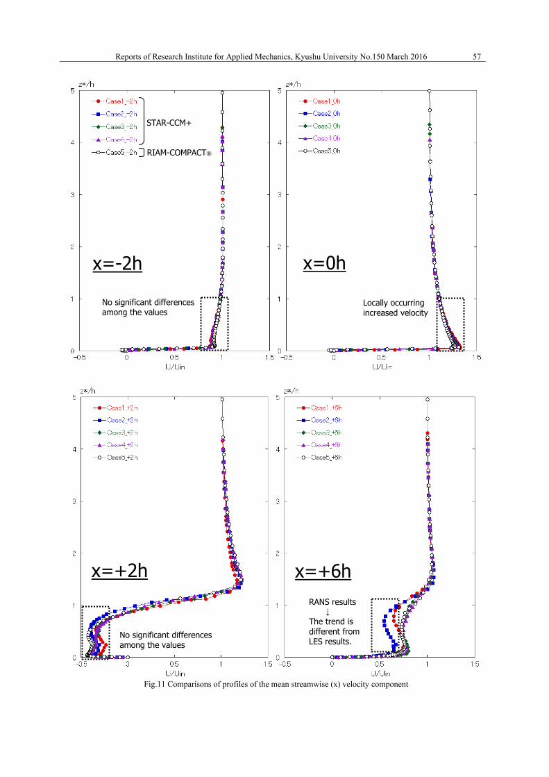
Subsequently, the vertical profiles of turbulence statistics

(the mean and standard deviation of the streamwise (x)

velocity component), shown in Figs.11 and 12, are examined.

The turbulence statistics were evaluated at a total of four

points, specifically, at x / h = -2, 0, +2, and +6 as shown in

Fig.10. In the mean velocity profiles, no significant

differences are found at any of the points given by x / h = -2,

0, and +2 (Fig.11). At the top of the isolated-hill, which is

located at x / h = 0, locally occurring increased wind velocity

is evident. Immediately downstream of the isolated-hill, that

is at x / h = +2, a region of reversed flow is present. At x/ h

= +6, the trends of the wind velocity profiles differ between

Flow


(a) Spalart-Allmaras single equation eddy-viscosity turbulence model, steady RANS

(b) SST k-ω two-equation eddy-viscosity model, unsteady RANS (URANS), time-averaged field

Fig.6 Distribution of the streamwise (x) velocity component; simulation results from STAR-CCM+ with the use of RANS

turbulence models. The cross-sections shown are for the central plane (y = 0) aligned with the streamwise direction (x).

Flow


(a) Standard Smagorinsky model, LES

(b) WALE model, LES

Fig.7 Distribution of the time-averaged streamwise (x) velocity component; simulation results from STAR-CCM+ with the use of

LES turbulence models. The cross-sections shown are for the central plane (y = 0) aligned with the streamwise direction (x).

Flow


(a) Spalart-Allmaras single equation eddy-viscosity turbulence model, steady RANS

(b) SST k-ω two-equation eddy-viscosity model, unsteady RANS (URANS), time-averaged field

Fig.8 Distribution of velocity vectors; simulation results from STAR-CCM+ with the use of RANS turbulence models.

The cross-sections shown are for the central plane (y = 0) aligned with the streamwise direction (x).

Flow

The vortex region is not simulated clearly.

The vortex region is not simulated clearly.


(a) Standard Smagorinsky model, LES

(b) WALE model, LES

Fig.9 Distribution of time-averaged velocity vectors; simulation results from STAR-CCM+ with the use of LES turbulence

models. The cross-sections shown are for the central plane (y = 0) aligned with the streamwise direction (x).

Flow

Vortex center

Vortex center


(a) Distribution of the streamwise (x) velocity component

(b) Distribution of velocity vectors

Fig.10 Time-averaged results from RIAM-COMPACT® with the use of the standard Smagorinsky LES model.

The cross-sections shown are for the central plane (y = 0) aligned with the streamwise direction (x).

Flow

-2h 0h +2h +6h

-2h 0h +2h +6h

height h

Vortex center

height h


Fig.11 Comparisons of profiles of the mean streamwise (x) velocity component

x=-2h x=0h

x=+2h x=+6h

RIAM-COMPACT®

STAR-CCM+

Locally occurring increased velocity

No significant differences among the values

RANS results ↓ The trend is different from LES results.

No significant differences among the values


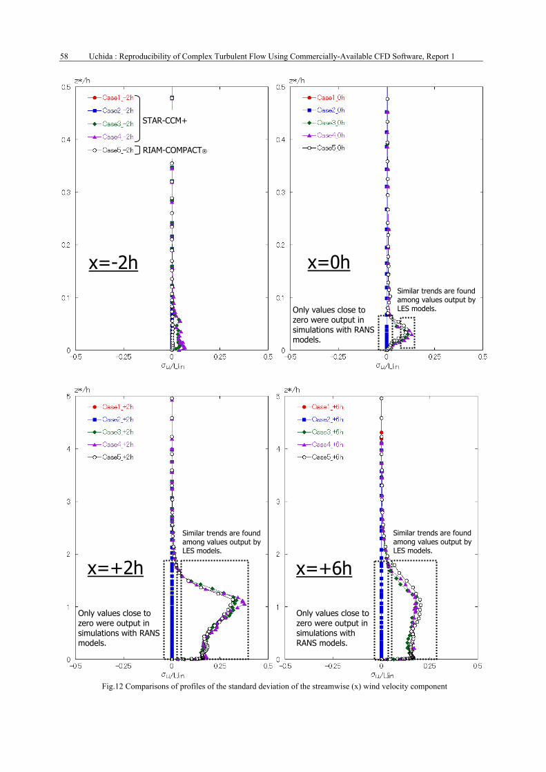
Fig.12 Comparisons of profiles of the standard deviation of the streamwise (x) wind velocity component

x=-2h x=0h

x=+2h x=+6h

STAR-CCM+

RIAM-COMPACT®

Only values close to zero were output in simulations with RANS models.

Similar trends are found among values output by LES models.






the simulation results from RANS models and those from

LES models.

From the point of view of predicting the airflow field over

complex terrain, these errors in the simulation results from

the RANS models would significantly affect assessments of

the power to be generated and other variables.

In the vertical profiles of the standard deviation of the

streamwise (x) wind velocity component predicted by the

RANS models, no significant differences are found at any of

the four examined points (Fig.12). Similarly, it can be said

that the trends of the profiles from simulations which used

the LES models, i.e., simulations by STAR-CCM+ with both

the standard Smagorinsky model and the WALE model and

the simulation by RIAM-COMPACT®, are nearly identical.

In the simulations performed in the present study, the

number of mesh points used in RIAM-COMPACT®

(structured mesh, approx. five million mesh points) is

approximately five times that used in STAR-CCM+

(unstructured mesh, approx. one million mesh points).

Nonetheless, it has been confirmed that the simulation by

RIAM-COMPACT® completes approximately ten times

faster than those by STAR-CCM+.

7. Conclusions

In the present paper, the airflow field in the vicinity of an

isolated-hill with steep slopes was simulated by one of the

leading, commercially-available CFD packages, STAR-

CCM+ as well as by RIAM-COMPACT® (turbulence model:

LES based on the standard Smagorinsky model). The

simulation results were compared to examine the prediction

accuracy of RIAM-COMPACT®. In STAR-CCM+, two

types of RANS turbulence models were selected: the

Spalart-Allmaras single equation eddy-viscosity turbulence

model (steady RANS) and the SST k-ω two-equation

eddy-viscosity model (unsteady RANS). In addition, for LES

turbulence models (SGS models), the standard Smagorinsky

model and the WALE model were selected.

From the comparisons of the simulation results, the

following have been found. Images visualizing the flow fields

time-averaged over the interval of t = 100 – 200 (h / U)

suggested that the trends of the simulation results from

STAR-CCM+ with the RANS turbulence models (steady and

unsteady) were quite similar to each other. In addition, the

trends of the flow patterns simulated by RIAM-COMPACT®

with the LES turbulence model (the standard Smagorinsky

model) and STAR-CCM+ with the LES turbulence models

(the standard Smagorinsky model and the WALE model)

were nearly the same. In addition, the center of the vortex

(region of reversed flow) downstream of the isolated-hill

which was evident in the LES simulations, was not

adequately simulated by STAR-CCM+ using the RANS

turbulence models.

In the present study, the vertical profiles of turbulence

statistics (the mean and standard deviation of the streamwise

(x) wind velocity component) were evaluated and compared

at four points, x / h = -2, 0, +2, and +6. The comparisons

revealed the following. No significant difference was found

among the mean velocity profiles obtained from all the

turbulence models at x / h = -2, 0, and +2. At the top of the

isolated-hill, which was located at x/h = 0, locally occurring

increased velocity was identified. At x / h = +2, which was

immediately downstream of the isolated-hill, an area of

negative velocity was found, indicating the presence of a

region of reversed flow. At x / h = +6, the trends of the

results differed between the simulations which used the

RANS models and those which used the LES models.

From the perspective of predicting the airflow field over

complex terrain, the prediction errors in the mean wind

velocity in the RANS model simulations would greatly affect

the assessments of the power to be generated and other

variables.

In the simulations which used the RANS turbulence

models, the values of the standard deviation were not

significantly different from zero throughout the profiles at all

the examined points. In the simulations which used the LES

models, i.e., STAR-CCM+ with the standard Smagorinsky

model and the WALE model and RIAM-COMPACT® with

the standard Smagorinsky model, the trends of the profiles of

the mean and standard deviation of the wind velocity

resembled one another quite closely as was the case for the

trends of the visualized flow field.

References 1) Takanori UCHIDA and Yuji OHYA, Micro-siting

technique for wind turbine generators by using

large-eddy simulation, Journal of Wind Engineering &

Industrial Aerodynamics, Vol.96, pp.2121-2138, 2008

2) Takanori UCHIDA, Validation Testing of the

Prediction Accuracy of the Numerical Wind Synopsis

Prediction Technique RIAM-COMPACT for the Case

of the Bolund Experiment –Comparison against a

Wind-Tunnel Experiment–, Reports of RIAM, Kyushu

University, No.147, pp.7-14, 2014

reproducibility of complex turbulent flow using ... · reproducibility of complex turbulent flow...

Documents