reproducing kernel hilbert spaces - bilkent university
TRANSCRIPT
REPRODUCING KERNEL HILBERT SPACES
a thesis
submitted to the department of mathematics
and the institute of engineering and science
of bilkent university
in partial fulfillment of the requirements
for the degree of
master of science
By
Baver Okutmustur
August, 2005
I certify that I have read this thesis and that in my opinion it is fully adequate,
in scope and in quality, as a thesis for the degree of Master of Science.
Assist. Prof. Dr. Aurelian Gheondea (Supervisor)
I certify that I have read this thesis and that in my opinion it is fully adequate,
in scope and in quality, as a thesis for the degree of Master of Science.
Prof. Dr. Mefharet Kocatepe
I certify that I have read this thesis and that in my opinion it is fully adequate,
in scope and in quality, as a thesis for the degree of Master of Science.
Assoc. Prof. Dr. H. Turgay Kaptanoglu
Approved for the Institute of Engineering and Science:
Prof. Dr. Mehmet B. BarayDirector of the Institute Engineering and Science
ii
ABSTRACT
REPRODUCING KERNEL HILBERT SPACES
Baver Okutmustur
M.S. in Mathematics
Supervisor: Assist. Prof. Dr. Aurelian Gheondea
August, 2005
In this thesis we make a survey of the theory of reproducing kernel Hilbert spaces
associated with positive definite kernels and we illustrate their applications for in-
terpolation problems of Nevanlinna-Pick type. Firstly we focus on the properties
of reproducing kernel Hilbert spaces, generation of new spaces and relationships
between their kernels and some theorems on extensions of functions and kernels.
One of the most useful reproducing kernel Hilbert spaces, the Bergman space, is
studied in details in chapter 3. After giving a brief definition of Hardy spaces, we
dedicate the last part for applications of interpolation problems of Nevanlinna-
Pick type with three main theorems: interpolation with a finite number of points,
interpolation with an infinite number of points and interpolation with points on
the boundary. Finally we include an Appendix that contains a brief recall of the
main results from functional analysis and operator theory.
Keywords: Reproducing kernel, Reproducing kernel Hilbert spaces, Bergman
spaces, Hardy spaces, Interpolation, Riesz theorem.
iii
OZET
DOGURAN CEKIRDEKLI HILBERT UZAYLARI
Baver Okutmustur
Matematik, Yuksek Lisans
Tez Yoneticisi: Yrd. Doc. Dr. Aurelian Gheondea
Agustos, 2005
Bu tezde, doguran cekirdekli Hilbert uzayları teorisini pozitif tanımlı
cekirdekler ile beraber inceledik ve bunun uygulamalarını Nevallina-Pick inter-
polasyon problemleri uzerinde ornekledik. Oncelikle, doguran cekirdekli Hilbert
uzaylarının ozelliklerini, uretilen yeni uzaylar ve onların cekirdekleri arasındaki
iliskileri ve genisletilen cesitli fonksiyon ve cekirdeklerle ilgili bazı teoremleri
inceledik. Sıkca kullanılan doguran cekirdekli Hilbert uzaylarından biri olan
Bergman uzayı 3. kısımda detaylarıyla islendi. Hardy uzayının kısa bir
tanımıyla basladıgımız son kısım, Nevallina-Pick interpolasyon problemlerinin
uygulamalarını iceren uc ana teorem ile son buldu. Bunlar: sınırlı sayıda nokta
ile interpolasyon, sınırsız sayıda nokta ile interpolasyon ve sınır noktalarında in-
terpolasyon. Son olarak Appendix kısmı bu tezde sıkca kullandıgımız fonksiyonel
analiz ve operator teori ile ilgili temel esasların kısa bir ozetine ayrıldı.
Anahtar sozcukler : Doguran cekirdekler, Doguran cekirdekli Hilbert uzayları,
Bergman uzayları, Hardy uzayları, Interpolasyon, Riesz teoremi.
iv

Acknowledgement
I would like to express my sincere gratitude to my supervisor Assoc. Prof.
Aurelian Gheondea, firstly for introducing me to this area of analysis, for his
excellent guidance, valuable suggestions, encouragement and infinite patience. I
am glad to have a chance to study with this great person who is a role model as
a supervisor and a mathematician.
My sincere thanks to Prof. Dr. Mefharet Kocatepe for her interest and useful
comments.
I also need to express my gratitude to Assoc. Prof. H. Turgay Kaptanoglu
for providing me necessary documents for this study.
I am grateful to Aslı Pekcan and Murat Altunbulak who helped me about
Latex. Special thanks to Aslı for reading my thesis, for her advices, corrections
and helps.
Beside, I would like to thank Serdar, Hikmet, Rohat, Ergun, Inan, Fatma,
Burcu, Sultan and all my friends who always cared about my work and increased
my motivation, which I have strongly needed.
I would like to thank Eliya Buyukkaya who has always been with me with her
endless love, support and understanding.
Finally, I would like to express my deepest gratitude for the constant support,
encouragement, trust and love that I received from my family.
v
Contents
1 Introduction 1
2 Reproducing Kernel Hilbert Spaces 4
2.1 Definition, Uniqueness and Existence . . . . . . . . . . . . . . . . 4
2.2 Operations with Reproducing Kernel Hilbert Spaces . . . . . . . . 15
2.3 Extension of Functions and Kernels . . . . . . . . . . . . . . . . . 25
3 Spaces of Analytic Functions 33
3.1 Sesqui-analytic kernels . . . . . . . . . . . . . . . . . . . . . . . . 33
3.2 Bergman Spaces . . . . . . . . . . . . . . . . . . . . . . . . . . . . 42
3.3 Szego Kernel . . . . . . . . . . . . . . . . . . . . . . . . . . . . . 48
4 Interpolation Theorems 60
4.1 General definition of Hardy spaces . . . . . . . . . . . . . . . . . . 60
4.2 Interpolation Inside Unit Disc . . . . . . . . . . . . . . . . . . . . 66
4.3 Interpolation on the Boundary . . . . . . . . . . . . . . . . . . . . 73
vi
CONTENTS vii
A Hilbert Spaces 76
A.1 Definitions . . . . . . . . . . . . . . . . . . . . . . . . . . . . . . . 76
A.2 Projection . . . . . . . . . . . . . . . . . . . . . . . . . . . . . . . 83
A.3 Weak Topology . . . . . . . . . . . . . . . . . . . . . . . . . . . . 88
A.4 Self-adjoint Operators . . . . . . . . . . . . . . . . . . . . . . . . 91
Chapter 1
Introduction
The reproducing kernel was used for the first time at the beginning of the 20th
century by S. Zaremba in his work on boundary value problems for harmonic and
biharmonic functions. In 1907, he was the first who introduced, in a particular
case, the kernel corresponding to a class of functions, and stated its reproducing
property. But he did not develop any theory and did not give any particular
name to the kernels he introduced.
In 1909, J. Mercer examined the functions which satisfy reproducing property
in the theory of integral equations developed by Hilbert and he called this func-
tions as ’positive definite kernels’. He showed that this positive definite kernels
have nice properties among all continuous kernels of integral equations.
However, for a long time these results were not investigated. Then the idea
of reproducing kernels appeared in the dissertations of three Berlin mathemati-
cians G. Szego (1921), S. Bergman (1922) and S. Bochner (1922). In particular,
S. Bergman introduced reproducing kernels in one and several variables for the
class of harmonic and analytic functions and he called them ’kernel functions’.
In 1935, E.H. Moore examined the positive definite kernels in his general
analysis under the name of positive Hermitian matrix.
Later, the theory of reproducing kernels was systematized by N.Aronszajn
1
CHAPTER 1. INTRODUCTION 2
around 1948.
The original idea of Zaremba to apply the kernels to the solution of boundary
value problems was developed by S. Bergman and M. Schiffer. In these investi-
gations, the kernels were proved to be powerful tool for solving boundary value
problems of partial differential equations of elliptic type. Moreover, by application
of kernels to conformal mapping of multiply-connected domains, very beautiful
results were obtained by S. Bergman and M. Schiffer.
Several important results were achieved by the use of these kernels in the
theory of one and several complex variables, in conformal mapping of simply-
and multiply-connected domains, in pseudo-conformal mappings, in the study of
invariant Riemannian metrics and in other subjects.
Meanwhile, in probability theory, the theory of positive definite kernels was
used by A.N. Kolmogorov, E. Parzen and others.
There are also several papers and lecture notes on this subject; B. Burbea
(1987), E. Hille (1972), S. Saitoh (1988), H. Dym (1989) and T. Ando (1987).
Most part of this thesis owes to T. Ando’s lecture notes [1] in its diversity of tools
and results. We also used H. Dym, S. Saitoh and N. Aronszajn’s works especially
for the second chapter. Moreover, we used partially the books of P.L. Duren [4],
P. Koosis [7], P.L. Duren and A. Schuster’s [5] for complementing with result on
Bergman and Hardy spaces.
The thesis is organized as follows:
In Chapter 2, after giving definitions and properties of reproducing kernel
Hilbert spaces with some theorems, we focus on generation of new spaces and
relationship between their kernels. Also, some extension theorems of functions
and kernels are proven.
In Chapter 3, we present some of the most useful reproducing kernel Hilbert
spaces consisting of analytic functions. A special role is played by the Bergman
spaces and Bergman kernels that we present in detail.
CHAPTER 1. INTRODUCTION 3
Chapter 4 is dedicated to applications to interpolation problems of
Nevanlinna-Pick type. We start with a brief definition of Hardy spaces. Then we
prove three main theorems: interpolation with a finite number of points, inter-
polation with an infinite number of points, and interpolation with points on the
boundary.
The Appendix part contains some elementary facts from functional analysis
and operator theory in Hilbert spaces which can be found in textbooks, e.g. in
J. Conway [3] and J. Weidman [9].
Chapter 2
Reproducing Kernel Hilbert
Spaces
2.1 Definition, Uniqueness and Existence
Definition 2.1.1. Let H be a Hilbert space of functions on a set X. Denote by
〈f, g〉 the inner product and let ‖f‖ = 〈f, f〉1/2 be the norm in H, for f and g ∈H. The complex valued function K(y, x) of y and x in X is called a reproducing
kernel of H if the followings are satisfied:
(i) For every x, Kx(y) = K(y, x) as a function of y belongs to H.
(ii) The reproducing property: for every x ∈ X and every f ∈ H,
f(x) = 〈f,Kx〉. (2.1)
So applying (2.1) to the function Kx at y, we get
Kx(y) = 〈Kx, Ky〉, for x, y ∈ X,
and by (i),
K(y, x) = 〈Kx, Ky〉, for x, y ∈ X.
By the above relations, for x ∈ X we obtain ‖Kx‖ = 〈Kx, Kx〉1/2 = K(x, x)1/2.
4
CHAPTER 2. REPRODUCING KERNEL HILBERT SPACES 5
Definition 2.1.2. A Hilbert space H of functions on a set X is called a repro-
ducing kernel Hilbert space (sometimes abbreviated by RKHS) if there exists a
reproducing kernel K of H, cf. Defintion 2.1.1.
The Hilbert space with reproducing kernel K is denoted by HK(X). Corre-
spondingly norm will be denoted by ‖ · ‖K (or sometimes by ‖ · ‖HK) and inner
product will be denoted by 〈·, ·〉K (or sometimes by 〈·, ·〉HK), if there is a need of
distinction.
Theorem 2.1.3. If a Hilbert space H of functions on a set X admits a repro-
ducing kernel, then the reproducing kernel K(y, x) is uniquely determined by the
Hilbert space H.
Proof. Let K(y, x) be a reproducing kernel of H. Suppose that there exists an-
other kernel K′(y, x) of H. Then, for all x ∈ X, applying (ii) for K and K ′ we
get
‖Kx −K ′x‖2 = 〈Kx −K ′
x, Kx −K ′x〉
= 〈Kx −K ′x, Kx〉 − 〈Kx −K ′
x, K′x〉
= (Kx −K ′x)(x)− (Kx −K ′
x)(x)
= 0
Hence Kx = K ′x, that is, Kx(y) = K ′
x(y) for all y ∈ X. This means that
K(x, y) = K ′(x, y) for all x, y ∈ X.
Theorem 2.1.4. For a Hilbert space H of functions on X, there exists a re-
producing kernel K for H if and only if for every x of X, the evaluation linear
functional H 3 f 7−→ f(x) is a bounded linear functional on H.
Proof. Suppose that K is the reproducing kernel for H. By reproducing property
and Schwarz inequality of the scalar product, for all x ∈ X,
|f(x)| = |〈f,Kx〉| ≤ ‖f‖‖Kx‖ = ‖f‖〈Kx, Kx〉1/2 = ‖f‖K(x, x)1/2
that is, the evaluation at x is a bounded linear functional on H.
CHAPTER 2. REPRODUCING KERNEL HILBERT SPACES 6
Conversely, if for all x ∈ X the evaluation H 3 f 7→ f(x) is a bounded linear
functional on H, then by the Riesz Representation Theorem, for all x ∈ X, there
exists a function gx belonging to H such that
f(x) = 〈f, gx〉.If we put Kx instead of gx, then for all y ∈ X, we get Kx(y) = gx(y). Hence K is
a reproducing kernel for H.
Definition 2.1.5. Let X be an arbitrary set and K be a kernel on X, that is,
K : X ×X → C. The kernel K is called Hermitian if for any finite set of points
y1, . . . , yn ⊆ X and any complex numbers ε1, . . . , εn we have
n∑i,j=1
εjεiK(yj, yi) ∈ R
and K is called positive definite ifn∑
i,j=1
εjεiK(yj, yi) ≥ 0.
Equivalently, the last inequality means that for any finitely supported family of
complex numbers εxx∈X we have∑
x,y∈X
εyεxK(y, x) ≥ 0. (2.2)
In brief, sometimes we will denote this by [K(y, x)] ≥ 0 on X, or equivalently, we
will say that K is a positive definite matrix in the sense of E. H. Moore.
Theorem 2.1.6. The reproducing kernel K(y, x) of a reproducing kernel Hilbert
space H is a positive matrix in the sense of E. H. Moore.
Proof. We have
0 ≤ ‖n∑
i=1
εiKyi‖2 = 〈
n∑i=1
εiKyi,
n∑j=1
εjKyj〉
=n∑
i=1
n∑j=1
εiεj〈Kyi, Kyj
〉 =n∑
i=1
n∑j=1
εiεjK(yj, yi).
Hence,n∑
i,j=1
K(yj, yi)εjεi ≥ 0.
CHAPTER 2. REPRODUCING KERNEL HILBERT SPACES 7
Remark 2.1.7. Given a reproducing kernel Hilbert space H and its kernel
K(y, x) on X, then for all x, y ∈ X we have the followings:
(i) K(y, y) ≥ 0.
(ii) K(y, x) = K(x, y).
(iii) |K(y, x)|2 ≤ K(y, y)K(x, x), (Schwarz Inequality).
(iv) Let x0 ∈ X. Then the followings are equivalent:
(a) K(x0, x0) = 0.
(b) K(y, x0) = 0 for all y ∈ X.
(c) f(x0) = 0 for all f ∈ H.
Indeed, (i) and (ii) can be easily seen. For (iii), we use the Schwarz Inequality
in H and get
|K(y, x)|2 = |〈Kx, Ky〉|2 ≤ ‖Kx‖‖Ky‖‖Kx‖‖Ky‖ = ‖Kx‖2‖Ky‖2
= 〈Kx, Kx〉〈Ky, Ky〉 = K(x, x)K(y, y)
which is the desired result.
As for (iv), it follows by (iii) that K(x0, x0) = 0 is equivalent with K(y, x0) = 0
for all y ∈ X. Further, by the reproducing property, K(y, x0) = 0 for all y ∈ X
if and only if f(x0) = 0, for all f .
The following theorem can be regarded as a converse of Theorem 2.1.3.
Theorem 2.1.8. For any positive definite kernel K(y, x) on X, there exists a
uniquely determined Hilbert space HK of functions on X, admitting the reproduc-
ing kernel K(y, x).
Proof. We denote by H0 the space of all functions f on X such that there exists
a finite set of points x1, x2, . . . , xn of X and complex numbers ε1, ε2, . . . , εn,
f(y) =n∑
i=1
εiK(y, xi),
CHAPTER 2. REPRODUCING KERNEL HILBERT SPACES 8
for all y ∈ X. Let g(·) =∑m
i=1 µjK(·, yj) be in H0. Define the inner product of
the functions f and g from H0 by
〈f, g〉H0 =n∑
i=1
m∑j=1
εiµj〈K(·, xi), K(·, yj)〉H0 =n∑
i=1
m∑j=1
εiµjK(yj, xi). (2.3)
Then,
〈f, K(·, x)〉H0 =n∑
i=1
εi〈K(·, xi), K(·, x)〉 =n∑
i=1
εiK(x, xi) = f(x) (2.4)
for all x ∈ X, that is, H0 has the reproducing property. This implies that the
definition of the inner product in (2.3) does not depend on the representations
of the functions f and g in H0. Moreover, it is easy to see that 〈·, ·〉H0 is linear
in the first variable and Hermitian. Since K is positive definite it follows that
〈f, f〉H0 ≥ 0 for all f ∈ H0, hence we have the Schwarz Inequality for 〈·, ·〉H0 . In
addition, if 〈f, f〉H0 = 0, ‖f‖ = 0 and then by (2.4) for all x ∈ X,
|f(x)| ≤ ‖f‖‖K(·, x)‖ = 0,
which implies that f ≡ 0. Thus, (H0, 〈·, ·〉H0) is a pre-Hilbert space.
Now denote by H abstract the completion of H0 to a Hilbert space. We will
show that H has a unique representation as a Hilbert space with reproducing
kernel K(y, x). Consider first any Cauchy sequence (fn)n≥1 in H0. Then for any
x ∈ X we have
|fm(x)− fn(x)| = |〈fm, Kx〉H0 − 〈fn, Kx〉H0|= |〈fm − fn, Kx〉H0|≤ ‖fm − fn‖H0K(x, x)1/2.
So, there exists the function f : X → C such that for all x ∈ X,
limn→∞
fn(x) = f(x). (2.5)
Moreover, we have
‖f‖H = limn→∞
‖fn‖H0
CHAPTER 2. REPRODUCING KERNEL HILBERT SPACES 9
and for any two Cauchy sequences (fn) and (gn) in H0, denoting by f and,
respectively g, the corresponding pointwise limit of (fn) and (gn), we have
〈f, g〉H = limn,m→∞
〈fn, gm〉H0 .
We can easily see that, for any two Cauchy sequences (fn) and (gn), these limits
exist and are independent of the approximating sequences (fn) and (gn) of the
limits f and g, respectively.
Let us note that (2.5) yields a concrete representation of H as a space of
functions on X. In addition, K has the reproducing property with respect to H.
To see this, let f ∈ H and (fn) ⊂ H such that fn → f as n →∞ strongly. Then
for all x ∈ X,
f(x) = limn→∞
fn(x) = limn→∞
〈fn, Kx〉H0
= 〈 limn→∞
fn, Kx〉H0 = 〈f,Kx〉H
It remains to show the uniqueness of the Hilbert space H admitting the repro-
ducing kernel K. Suppose H1 is another Hilbert space with the same reproducing
kernel K. By definition, for any x ∈ X, Kx ∈ H1 and then we have H0 ⊆ H1.
Also, for any f, g ∈ H0, because of the reproducing property we have
〈f, g〉H0 = 〈f, g〉H1 . (2.6)
If f ∈ H1 such that 0 = 〈f, Kx〉H1 = f(x) for all x ∈ X, then f ≡ 0. Thus, the
family Kx : x ∈ X is total in H1. So for any f ∈ H1, we can take a Cauchy
sequence (fn)n≥1 in H0 such that limn→∞
fn = f. Hence, (2.6) is valid in H0.
Now since we have H0 ⊆ H1 and (2.6), we obtain H ⊆ H1. Also from the
construction of H, we get H1 ⊆ H. Thus, we have H1 = H.
Finally, we have to show that the inner products and the norms are equal in
H and H1. Consider any f, g ∈ H1 and any Cauchy sequences (fn)n≥1 and (gn)n≥1
in H0 which converge to f and g respectively. We have
〈f, g〉H1 = limn→∞
〈fn, gn〉H1 = limn→∞
〈fn, gn〉H0 = 〈f, g〉H
and hence the norms in H and H1 are equal.
CHAPTER 2. REPRODUCING KERNEL HILBERT SPACES 10
Theorem 2.1.9. Every sequence of functions (fn)n≥1 which converges strongly
to a function f in HK(X), converges also in the pointwise sense, that is,
limn→∞
fn(x) = f(x), for any point x ∈ X. Further, this convergence is uniform
on every subset of X on which x 7−→ K(x, x) is bounded.
Proof. For x ∈ X, using the reproducing property and the Schwartz Inequality,
|f(x)− fn(x)| = |〈f,Kx〉 − 〈fn, Kx〉|= |〈f − fn, Kx〉‖≤ ‖f − fn‖ · ‖Kx‖= ‖f − fn‖ ·K(x, x)1/2.
Therefore, limn→∞
fn(x) = f(x), for any point x ∈ X.
Moreover, it is clear from the above inequality that this convergence is uniform
on every subset of X on which x 7−→ K(x, x) is bounded.
In the following we will use the following notation: given X an abstract
nonempty set and H and K two Hermitian kernels on X, we denote
[H(y, x)] ≤ [K(y, x)] on X, (2.7)
whenever for any natural number n, any finite set x1, . . . , xn ⊆ X and any
complex numbers ε1, . . . , εn we have
n∑i,j=1
εjεiH(xj, xi) ≤n∑
i,j=1
εjεiK(xj, xi). (2.8)
Theorem 2.1.10. A complex valued function g on X belongs to the reproducing
kernel Hilbert space HK(X) if and only if there exists 0 ≤ γ < ∞ such that,
[g(y)g(x)] ≤ γ2[K(y, x)] on X. (2.9)
The minimum of all such γ coincides with ‖g‖.
Proof. By the reproducing property, g ∈ HK and ‖g‖ ≤ γ is equivalent with the
existence of f ∈ HK(X) such that ‖f‖ ≤ γ and g(x) = 〈f,Kx〉 for x ∈ X. By
CHAPTER 2. REPRODUCING KERNEL HILBERT SPACES 11
applying the Abstract Interpolation Theorem (see Theorem A.2.6) we obtain the
inequality (2.9). The converse implication is also a consequence of the Abstract
Interpolation Theorem.
Theorem 2.1.11. Let K(1)(y, x) and K(2)(y, x) be two positive definite kernels
on X. Then the following assertions are mutually equivalent:
(i) HK(1)(X) ⊆ HK(2)(X), (set inclusion).
(ii) There exists 0 ≤ γ < ∞ such that
[K(1)(y, x)] ≤ γ2[K(2)(y, x)].
If this is the case, the inclusion map J in (i) is continuous, and its norm is given
by the minimum of γ in (ii).
Proof. Denote the norm and the inner product in HK(i)(X) by ‖ · ‖i and 〈·, ·〉i,respectively.
Let (i) be satisfied. Set J : HK(1)(X) −→ HK(2)(X), the inclusion map.
Claim: J is a closed and continuous operator.
Suppose that fn → g in HK(1)(X) and fn → h in HK(2)(X). As point evalua-
tions are continuous in HK(i)(X), (i = 1, 2), we get
fn(x) → g(x) and fn(x) → h(x)
which implies that g(x) = h(x) for all x, since the limit is unique. So J is closed.
Since J is closed, we know that by the Closed Graph Theorem any closed linear
operator between Hilbert spaces is continuous. Hence J is continuous, as claimed.
Now, for all f ∈ HK(1)(X) and for all x ∈ X, by reproducing property we
have f(x) = 〈f, K(1)x 〉1 and (Jf)(x) = 〈Jf,K
(2)x 〉2. Then by using this and the
inclusion property of J , for all x ∈ X, we have
〈f, J∗K(2)x 〉1 = 〈Jf,K(2)
x 〉2 = (Jf)(x) = 〈f,K(1)x 〉1
CHAPTER 2. REPRODUCING KERNEL HILBERT SPACES 12
and hence we obtain J∗K(2)x = K
(1)x for all x ∈ X.
Finally, for any γ ≥ ‖J‖ and any finitely supported family of complex numbers
εxx∈X , we have∑x,y
εxεyK(1)(y, x) = 〈
∑x
εxK(1)x ,
∑y
εyK(1)y 〉 = ‖
∑x
εxK(1)x ‖2
1
= ‖J∗(∑
x
εxK(2)x )‖2
1 ≤ γ2‖∑
x
εxK(2)x ‖2
= γ2〈∑
x
εxK(2)x ,
∑y
εyK(2)y 〉
= γ2∑x,y
εxεyK(2)(y, x)
Hence,
[K(1)(y, x)] ≤ γ2[K(2)(y, x)].
Conversely, suppose that (ii) is satisfied for some 0 ≤ γ < ∞. This means that
for any finitely supported family of complex numbers εxx∈X , that is denoted
by [εx], ∑x,y
εxεyK(1)(y, x) ≤ γ2
∑x,y
εxεyK(2)(y, x).
Taking the minimum of γ in Theorem 2.1.10, we have the norm of any function
f on X given by
‖f‖2i = sup
[εx]
|∑x εxf(x)|2∑x,y εxεyK(i)(y, x)
, (i = 1, 2),
with ‖f‖i = ∞ if f is not in HK(i)(X). Now since K(i)x : x ∈ X is total in
HK(i)(X), (i = 1, 2) and using the Schwarz Inequality for the norms ‖f‖1 and
‖f‖2, we get
‖f‖2 ≤ γ‖f‖1 for f ∈ HK(1)(X).
Hence, HK(1)(X) ⊆ HK(2)(X) with ‖J‖ ≤ γ.
Suppose that there is a map φ from a set X to a Hilbert space H such that
x 7−→ φx. Then φ can be used to define a positive definite kernel
K(y, x) = 〈φx, φy〉 for x, y ∈ X. (2.10)
CHAPTER 2. REPRODUCING KERNEL HILBERT SPACES 13
Theorem 2.1.12. Let φ : X 7−→ H and K be defined as in (2.10). Let T be the
linear operator from H to the space of functions on X, defined by
(Tf)(x) = 〈f, φx〉 for x ∈ X, f ∈ H.
Then Ran(T ) coincides with HK(X) and
‖Tf‖K = ‖PMf‖ for f ∈ H,
whereM is the orthogonal complement of ker(T ), PM is the orthogonal projection
onto M and ‖ · ‖K denotes the norm in HK(X).
Proof. To see the positive definiteness of K(y, x), let X 3 x 7−→ εx be a complex
valued function with finite support. Then,
∑x,y
εyεxK(y, x) =∑x,y
εyεx〈φx, φy〉 =∑x,y
〈εxφx, εyφy〉
= 〈∑
x
εxφx,∑
y
εyφy〉 = ‖∑
x
εxφx‖2 ≥ 0 for x, y ∈ X.
Hence K(y, x) is positive definite.
Let x ∈ X and Kx : X −→ C. For all y ∈ X, Kx(y) = 〈φx, φy〉 = (Tφx)(y). So,
Ran(T ) contains all the functions Kx, x ∈ X, where Kx(y) = K(y, x) = 〈φx, φy〉,y ∈ X. Since Ran(T ) is a linear space, then linear span of Kx : x ∈ X, that is,
linKx : x ∈ X = H0, will be in Ran(T ), i.e. H0 ⊆ Ran(T ).
Claim: T : linφx : x ∈ X −→ H0 is isometric.
Since Tφx = Kx, for all x ∈ X, then T (∑
x εxφx) =∑
x εxKx. Hence,
〈T (∑
x
εxφx), T (∑
y
ηyφy)〉K = 〈∑
x
εxKx,∑
y
ηyKy〉K =∑x,y
ηyεxK(y, x)
=∑x,y
ηyεx〈φx, φy〉H = 〈∑
x
εxφx,∑
y
ηyφy〉H.
That is, T linφx : x ∈ X −→ linKx : x ∈ X = H0 is isometric. Clearly,
T (linφx : x ∈ X) = H0.
CHAPTER 2. REPRODUCING KERNEL HILBERT SPACES 14
Now take f in ker(T ). So Tf = 0, i.e. (Tf)(x) = 0 for all x ∈ X. But
(Tf)(x) = 〈f, φx〉 = 0 for all x ∈ X and T is linear which implies
f ⊥ linφx : x ∈ X.
If f ∈ linφx : x ∈ X⊥ = φx : x ∈ X⊥, then for all x ∈ X,
0 = 〈f, φx〉 = (Tf)(x).
That is, Tf = 0 and ker(T ) = linφx : x ∈ X⊥. By this, we reach
ker(T )⊥ = lin φx : x ∈ X⊥⊥ = linφx : x ∈ X =: M.
As M is a closed subspace, then H can be written as H = M⊕M⊥. Since
T : linφx : x ∈ X −→ H0 ⊆ HK(X)
is isometric and surjective and since H0 is dense in HK(X), it follows that
T (linφx : x ∈ X) −→ H0 = HK(X). Hence, TM = HK(X) = T (M⊕M⊥) =
TH = Ran(T ).
Finally, to see the equality of norms, take f ∈ H = M⊕M⊥. It can be
written as f = PMf + (I − PM)f, where I − PM = PkerT . Then, since T is
isometric on M,
‖Tf‖K = ‖T (PMf + PkerT f)‖K = ‖TPMf‖K = ‖PMf‖K .
The next result that concludes this section shows that the assumptions in
(2.10) is by no means restrictive, if we consider positive definite kernels.
Theorem 2.1.13. (Kolmogorov Decomposition) Let K(y, x) be a positive
definite kernel on an abstract set X. Then there exists a Hilbert space H and a
function φ : X → H such that
K(y, x) = 〈φx, φy〉 for x, y ∈ X.
In addition, the Hilbert space H can be chosen in such a way that the set φxx∈X
is total in H and in this case the pair (φ,H) is unique in the following sense:
for any other pair (ψ,K), where ψ : X → K and K is a Hilbert space such that
ψxx∈X is total in K and K(y, x) = 〈ψx, ψy〉K for all x, y ∈ X, there exists a
unitary operator U ∈ L(H,K) such that Uφx = ψx for all x ∈ X.
CHAPTER 2. REPRODUCING KERNEL HILBERT SPACES 15
Proof. Since K is positive definite, by Theorem 2.1.8 there exists the reproducing
kernel space HK with reproducing kernel K. Let φx = Kx ∈ HK for all x ∈ X.
By the reproducing property, for all x, y ∈ X we have
K(y, x) = 〈Kx, Ky〉HK,
and Kxx∈X is a total subset of HK .
To prove uniqueness, let (ψ,K) be a pair as in the statement and define
Uφx = ψx for all x ∈ X. Clearly U extends by linearity as a linear mapping
U : linφx : x ∈ X → linψx : x ∈ X. In addition, for any finitely supported
families of complex numbers εxx∈X and ηyy∈X we have
〈U(∑x∈X
εxφx
), U
(∑y∈X
ηyφy
)〉K = 〈(∑x∈X
εxψx
),(∑
y∈X
ηyψy
)〉K
=∑
x,y∈X
εyεx〈ψx, ψy〉K
=∑
x,y∈X
εyεxK(y, x) =∑
x,y∈X
εyεx〈φx, φy〉HK
= 〈(∑x∈X
εxφx
),(∑
y∈X
ηyφy
)〉HK
which shows that U is isometric. Due to the fact that both families φxx∈X and
ψyy∈X are total in HK and, respectively, K, it follows that U can be uniquely
extended to a unitary operator U : HK → K. By definition, U satisfies the
condition Uφx = ψx for all x ∈ X.
2.2 Operations with Reproducing Kernel Hilbert
Spaces
Let K(y, x) be a positive definite kernel on X and H = HK(X) be the RKHS.
Let M be a closed subspace of HK(X). We know M is a Hilbert space since it is
closed. As every point evaluation functional is continuous in HK(X) and M is a
closed subspace, then every point evaluation functional is continuous also in M.
Thus, M is a RKHS.
CHAPTER 2. REPRODUCING KERNEL HILBERT SPACES 16
Denote by PM the orthogonal projection onto M. This means that, for h ∈HK(X), PM(h) = hM ∈ M where h = hM + hM⊥ , with hM ∈ M, hM⊥ ∈ M⊥.
If PMKx ∈ M, we have f(x) = 〈f, PMKx〉 for all f ∈ M. Then we have the
reproducing kernel KM(y, x) for M as
KM(y, x) = 〈PMKx, PMKy〉 = 〈PMP ∗MKx, Ky〉 = 〈PMKx, Ky〉.
Let K(0)(y, x) be the restriction of K(y, x) to a subset X0 of X, i.e. K(0)(y, x) =
K(y, x) |X0×X0 . Since K(y, x) is positive definite, then so is K(0)(y, x). Then by
Theorem 2.1.8 there exists a unique RKHS admitting K(0)(y, x) as its reproduc-
ing kernel. Denote this RKHS by HK(0)(X). The following theorem gives the
relation between HK(X) and HK(0)(X).
Theorem 2.2.1. Let K(0)(y, x) be the restriction of K(y, x) to a subset X0 of X,
HK(0)(X) be the RKHS admitting K(0)(y, x) as its reproducing kernel and HK(X)
be the RKHS with its reproducing kernel K(y, x). Then
HK(0)(X0) = f |X0 : f ∈ HK(X) (2.11)
and
‖h‖K(0) = min‖f‖K : f |X0 = h for h ∈ HK(0)(X0). (2.12)
Proof. For x, y ∈ X0, we have
K(0)(y, x) = K(y, x) and so 〈K(0)x , K(0)
y 〉K(0) = 〈Kx, Ky〉K .
Define a map S such that SK(0)x = Kx for all x ∈ X0, which is uniquely extended
to an isometry from the closed linear span of K0x : x ∈ X0 that coincides with
HK(0)(X0) onto the closed linear span M of Kx : x ∈ X0.
Let T = SPM where PM is the orthogonal projection to M, i.e. PM :
HK(X) −→M. We have
T : HK(X) = M⊕M⊥ −→ HK(0)(X0).
Since
(TKx)(y) = K(0)x (y) = Kx(y) for x, y ∈ X0,
CHAPTER 2. REPRODUCING KERNEL HILBERT SPACES 17
then
(Tf)(y) = f(y) for f ∈M and y ∈ X0
and when (Tf)(y) = 0, (Tf)(y) = f(y) = 〈f, Ky〉 = 0 for f ∈M⊥ and y ∈ X0.
So T is the restriction map to X0 and
(Tf)(x) = 〈Tf,K(0)x 〉K(0) = 〈f, T ∗K(0)
x 〉K , for x ∈ X0.
Hence we have (Tf)(x) = 〈f, φx〉 = 〈f, T ∗K(0)x 〉K which gives us φx = T ∗K(0)
x . By
this with Theorem 2.1.12 and taking into account that T ∗ is isometric,
〈φx, φy〉K = 〈T ∗K(0)x , T ∗K(0)
y 〉K = 〈K(0)x , K(0)
y 〉K(0) = K(0)(y, x),
for all x, y ∈ X0.
Let K(1)(y, x) and K(2)(y, x) be two positive definite kernels. Then
K(y, x) = K(1)(y, x) + K(2)(y, x)
is also a positive definite kernel.
LetHK(1) ,HK(2) andHK be RKHSs with reproducing kernels K(1)(y, x), K(2)(y, x)
and K(y, x), respectively, with K = K(1) + K(2).
Theorem 2.2.2. Let K(1)(y, x) and K(2)(y, x) be two positive definite kernels
and K = K(1) + K(2). Then
HK(X) = HK(1)(X) +HK(2)(X), (algebraic sum)
and for f ∈ HK(1)(X) and g ∈ HK(2)(X),
‖f + g‖2K = min‖f + h‖2
K(1) + ‖g − h‖2K(2) : h ∈ HK(1)(X) ∩HK(2)(X). (2.13)
Proof. We have
K(y, x) = K(1)(y, x) + K(2)(y, x) = 〈K(1)x , K(1)
y 〉K(1) + 〈K(2)x , K(2)
y 〉K(2) .
Consider the direct sum Hilbert space H = HK(1)⊕HK(2) . Since both HK(1)and
HK(2) are Hilbert spaces, so is H. Then, by the definition of inner product for
direct sum, we have
〈Kx, Ky〉K = K(y, x) = K(1)(y, x) + K(2)(y, x) = 〈K(1)x ⊕K(2)
x , K(1)y ⊕K(2)
y 〉K .
CHAPTER 2. REPRODUCING KERNEL HILBERT SPACES 18
Consider the map φ such that φ(x) = K(1)x ⊕K
(2)x . Then we have
K(y, x) = 〈K(1)x ⊕K(2)
x , K(1)y ⊕K(2)
y 〉K = 〈φx, φy〉.
Using the operator T in Theorem 2.1.12, where (Tf)(x) = 〈f, φx〉, we get
(T (f⊕g))(x) = 〈f⊕g, φx〉 = 〈f⊕g, K(1)x ⊕K(2)
x 〉K= 〈f, K(1)
x 〉K(1) + 〈g, K(2)x 〉K(2)
= f(x) + g(x).
So, T (f⊕g) = f + g. This shows by Theorem 2.1.12 that HK(X) = Ran(T ) =
HK(1)(X) +HK(2)(X). Again by the same theorem,
‖f + g‖2 = ‖PM(f⊕g)‖2, where M = (ker(T ))⊥.
Next we show that
ker(T ) = h⊕ (−h) : h ∈ HK(1)(X) ∩HK(2)(X).
If h ∈ HK(1)(X) ∩ HK(2)(X), then T (h ⊕ (−h)) = h − h = 0. Conversely, if
h1 ⊕ h2 ∈ ker(T ), then 0 = T (h1 ⊕ h2) = h1 + h2 implies that h2 = −h1. Thus
h ∈ HK(1)(X) ∩HK(2)(X).
Then by Theorem 2.1.12 we have M = (ker(T ))⊥ which implies M⊥ =
ker(T ). So, h⊕(−h) ∈M⊥. Consider the quotient
H/M⊥ := h +M⊥ : h ∈ H.
Let f ∈ HK(1)(X), g ∈ HK(2)(X) and f⊕g ∈ H = HK(1)⊕HK(2) . Then, for
k ∈ H/M⊥,
k = k + h : h ∈ M⊥,where k = f⊕g ∈ H, h = h⊕(−h) ∈M⊥. Then,
h = f⊕g + h⊕(−h) : f⊕g ∈ H, h⊕(−h) ∈M⊥.
Taking the norm of both sides, it follows that
‖h‖ = inf‖f⊕g + h⊕(−h)‖ : f⊕g ∈ H, h⊕(−h) ∈M⊥ = ‖PMk‖= ‖PM(f⊕g)‖ = ‖f + g‖.
CHAPTER 2. REPRODUCING KERNEL HILBERT SPACES 19
Taking the square, we get
‖f + g‖2 = inf‖f⊕g + h⊕(−h)‖2 : f⊕g ∈ H, h⊕(−h) ∈M⊥.
Then,
‖f⊕g + h⊕(−h)‖2 = 〈f⊕g + h⊕(−h), f⊕g + h⊕(−h)〉= 〈f⊕g, f⊕g〉+ 〈f⊕g, h⊕(−h)〉+ 〈h⊕(−h), f⊕g〉+ 〈h⊕(−h), h⊕(−h)〉= 〈f, f〉+ 〈g, g〉+〈f, h〉+ 〈g,−h〉+ 〈h, f〉+ 〈−h, g〉+ 〈h, h〉+ 〈−h,−h〉= ‖f + h‖2 + ‖g − h‖2.
Hence, we get
‖f + g‖2 = min‖f + h‖2 + ‖g − h‖2 : f ∈ HK(1)(X), g ∈ HK(2)(X),
h ∈ HK(1)(X) ∩HK(2)(X).
Given Hilbert spaces HK(1)(X) and HK(2)(X), the intersection HK(1)(X) ∩HK(2)(X) will be again a Hilbert space of functions on X with respect to the
norm
‖f‖2 := ‖f‖2K(1) + ‖f‖2
K(2) .
Since every point evaluation functional is continuous in both HK(1)(X) and
HK(2)(X), letting f ∈ HK(1)(X)∩HK(2)(X), it follows that every point evaluation
functional will be continuous in HK(1)(X)∩HK(2)(X). Therefore the intersection
Hilbert space is a RKHS.
Theorem 2.2.3. The reproducing kernel of the space
HK(X) = HK(1)(X) ∩HK(2)(X)
is determined, as a quadratic form, by
∑x,y
εyεxK(y, x) = inf∑
x,y
ηyηxK(1)(y, x) +
∑x,y
ζyζxK(2)(y, x) : [εx] = [ηx] + [ζx]
,
where [εx] is an arbitrary complex valued function on X with finite support, and
the same are true for [ηx] and [ζx].
CHAPTER 2. REPRODUCING KERNEL HILBERT SPACES 20
Proof. Consider the isometric map S, such that it embeds HK(X) into the direct
sum Hilbert space HK(1)(X)⊕HK(2)(X), S : HK(X) −→ HK(1)(X)⊕HK(2)(X)
that is
Sf = f⊕f for f ∈ HK(X).
Let PM be the orthogonal projection onto Ran(S) := M. Then PM = SS∗, and
by using the reproducing and algebraic direct sum properties, it follows
(Sf)(x) = 〈Sf, K(1)x ⊕K(2)
x 〉 = 〈f ⊕ f,K(1)x ⊕K(2)
x 〉= 〈f,K(1)
x 〉K(1) + 〈f, K(2)x 〉K(2)
= f(x) + f(x) = 2f(x) where f ∈ HK(X).
So, 〈Sf, K(1)x ⊕K
(2)x 〉 = 2f(x), i.e. 1
2〈Sf,K
(1)x ⊕K
(2)x 〉 = f(x). This implies
1
2〈f, S∗(K(1)
x ⊕K(2)x )〉 = f(x)
or equivalently
〈f,1
2S∗(K(1)
x ⊕K(2)x )〉 = f(x).
In other words, Kx = 12S∗(K(1)
x ⊕ K(2)x ) for x ∈ X. Then using this and the
isometricity of S,
∑x,y
εyεxK(y, x) = ‖∑
x
εxKx‖2K = ‖
∑x
εx1
2S∗(K(1)
x ⊕K(2)x )‖2
= ‖1
2SS∗
∑x
εx(K(1)x ⊕K(2)
x )‖2
= ‖PM(∑
x
εx(K(1)x ⊕K(2)
x ))‖2.
Now, since M = Ran(S) = (ker(S))⊥, then M = (K(1)x ⊕ (−K
(2)x ) : x ∈ X)⊥
which implies
M⊥ = [K(1)x ⊕ (−K(2)
x ) : x ∈ X]⊥⊥
= linK(1)x ⊕ (−K
(2)x ) : x ∈ X
= K(1)x ⊕ (−K(2)
x ) : x ∈ X.
CHAPTER 2. REPRODUCING KERNEL HILBERT SPACES 21
So, the elements of the form 12
∑x λx(K
(1)x ⊕ (−K
(2)x )) are dense in M⊥. Then,
by using Theorem 2.1.12 and the property of orthogonal projection, we get
‖PM(1
2
∑x
εx(K(1)x ⊕K(2)
x ))‖2
= ‖1
2
∑x
εx(K(1)x ⊕K(2)
x )⊕ 1
2
∑x
εx(K(1)x ⊕K(2)
x )‖2
= 〈12
∑x
εx(K(1)x ⊕K(2)
x )⊕ 1
2
∑x
εx(K(1)x ⊕K(2)
x ),
1
2
∑x
εx(K(1)x ⊕K(2)
x )⊕ 1
2
∑x
εx(K(1)x ⊕K(2)
x )〉
= 〈12
∑x
εx(K(1)x ⊕K(2)
x ),1
2
∑x
εx(K(1)x ⊕K(2)
x )〉
+ 〈12
∑x
εx(K(1)x ⊕K(2)
x ),1
2
∑x
εx(K(1)x ⊕K(2)
x )〉
= ‖1
2
∑x
εx(K(1)x ⊕K(2)
x )‖2 + ‖1
2
∑x
εx(K(1)x ⊕K(2)
x )‖2
=1
2‖
∑x
εx(K(1)x ⊕K(2)
x )‖2.
Let 12(εx + λx) = ηx,
12(εx − λx) = δx and 1
2(εx + λx) + 1
2(εx − λx) = εx, that is,
[εx] = [ηx] + [δx].
Finally, applying Theorem 2.2.2 to the function 12
∑x εx(K
(1)x ⊕K
(2)x ), we get
1
2‖
∑x
εx(K(1)x ⊕K(2)
x )‖2 = inf[λx]‖(
∑x
1
2(εx + λx)Kx
)⊕ (∑x
1
2(εx − λx)Kx
)‖2
where
‖(∑
x
1
2(εx + λx)Kx
)⊕ (∑x
1
2(εx − λx)Kx
)‖2
= ‖(∑
x
ηxK(1)x )⊕ (
∑x
δxK(2)x )‖2
= 〈∑
x
ηxK(1)x ⊕
∑x
δxK(2)x ,
∑x
ηxK(1)x ⊕
∑x
δxK(2)x 〉
= ‖∑
x
ηxK(1)x ‖2
K(1) + ‖∑
x
δxK(2)x ‖2
K(2)
=∑x,y
ηyηxK(1)(y, x) +
∑x,y
δyδxK(2)(y, x)
which completes the proof.
CHAPTER 2. REPRODUCING KERNEL HILBERT SPACES 22
Remark 2.2.4. Consider the tensor product Hilbert space HK(1)(X)⊗HK(2)(X).
Take g ∈ HK(1)(X), h ∈ HK(2)(X) and x, x′ ∈ X. It follows
(g ⊗ h)(x, x′) = g(x)h(x′) = 〈g, K(1)x 〉〈h,K
(2)x′ 〉 = 〈g ⊗ h,K(1)
x ⊗K(2)x′ 〉
which shows that the tensor product Hilbert space HK(1)(X) ⊗ HK(2)(X) is a
RKHS on X ×X.
Consider the map φ : X −→ HK(1)(X)⊗HK(2)(X) defined by x 7→ K(1)x ⊗K
(2)x .
Then
K(y, x) = 〈φx, φy〉 = 〈K(1)x ⊗K(2)
x , K(1)y ⊗K(2)
y 〉= 〈K(1)
x , K(1)y 〉 · 〈K(2)
x , K(2)y 〉
= K(1)(y, x) ·K(2)(y, x) for x, y ∈ X.
Hence the pointwise product of two positive definite kernels is again a positive
definite kernel.
Theorem 2.2.5. For the product kernel K(y, x) = K(1)(y, x) · K(2)(y, x), the
RKHS HK(X) consists of all functions f on X for which there are sequences
(gn)n≥0 of functions in HK(1)(X) and (hn)n≥0 of functions in HK(2)(X) such that
∞∑1
‖gn‖2K(1)‖hn‖2
K(2) < ∞ and∞∑1
gn(x)hn(x) = f(x) for all x ∈ X, (2.14)
and the norm is given by
‖f‖2K = min
∞∑1
‖gn‖2K(1)‖hn‖2
K(2)
,
where the minimum is taken over the set of all sequences (gn)n≥0 and (hn)≥0
satisfying (2.14).
Proof. Let T be an operator from HK(1) ⊗HK(2) to the space of functions on X,
associated with φx, as in Theorem 2.1.12 more precisely,
T : HK(1) ⊗HK(2) −→ F(X ) := f : X −→ C : f complex function on X.
CHAPTER 2. REPRODUCING KERNEL HILBERT SPACES 23
Let F ∈ HK(1) ⊗HK(2) . Then F will be of the form
F =∞∑1
gn ⊗ hn with gn ∈ HK(1) and hn ∈ HK(2) .
Let x ∈ X and φx := K(1)x ⊗ K
(2)x , φx : X −→ HK(1) ⊗ HK(2) and K(y, x) =
〈φx, φy〉.
It follows by Theorem 2.1.12
(TF )(x) = 〈F, φx〉 = 〈F, K(1)x ⊗K(2)
x 〉 = 〈∞∑
n=1
gn ⊗ hn, K(1)x ⊗K(2)
x 〉
=∞∑
n=1
〈gn, K(1)x 〉〈hn, K
(2)x 〉
=∞∑
n=1
gn(x)hn(x) = f(x).
Finally,
‖F‖2 = 〈F, F 〉 = 〈∞∑
n=1
gn ⊗ hn,
∞∑n=1
gn ⊗ hn〉
=∞∑
n=1
〈gn, gn〉K(1)〈hn, hn〉K(2)
=∞∑
n=1
‖gn‖2K(1)‖hn‖2
K(2) .
Taking the norm of (TF )(x) = f(x), again by Theorem 2.1.12 we get
‖f(x)‖K = ‖TF‖K = ‖PMF‖K = min ∞∑
1
‖gn‖2K(1)‖hn‖2
K(2)
.
Remark 2.2.6. If X consists of a finite number of points, say n, then the space of
all functions on X, that is Cn, has the canonical RKHS structure (l2n, 〈·, ·〉), where
the point evaluation at i is induced by the inner product with ei, (i = 1, 2, . . . , n).
Moreover, for a positive definite kernel K(j, i) on X, we have
K(j, i) = 〈Lei, ej〉, (i, j = 1, 2, . . . , n) (2.15)
where L is a uniquely determined linear operator on l2n and is positive definite.
CHAPTER 2. REPRODUCING KERNEL HILBERT SPACES 24
Theorem 2.2.7. If K(j, i) is a strictly positive definite kernel on X =
1, 2, . . . , n and the operator L on l2n is defined as in (2.15), then L is a strictly
positive definite operator and
〈f, g〉K = 〈L−1f, g〉 for f, g ∈ Cn. (2.16)
Proof. Given K(j, i) a positive definite kernel on X = 1, 2, . . . , n, consider the
inclusion map J : HK(X) −→ Cn = l2n. As a result of Theorem 2.1.11, J is
continuous.
Let J∗ be the adjoint of J. We have J∗ : l2n −→ HK(X). Let J∗(ei) = Ki,
(i = 1, 2, . . . , n). By (2.15),
〈Lei, ej〉 = K(j, i) = 〈Ki, Kj〉K = 〈J∗ei, J∗ej〉K = 〈(JJ∗ei), ej〉
which gives
L = JJ∗.
Since K is a strictly positive definite kernel, it follows that dim(HK(X)) = n and
J is a bijection. Hence,
〈f, g〉K = 〈J−1f, J−1g〉K = 〈(J−1)∗J−1f, g〉= 〈(JJ∗)−1f, g〉 = 〈L−1f, g〉
and consequently we have
〈f, g〉K = 〈L−1f, g〉.
Each positive definite operator L on l2n produces a positive definite kernel
K(j, i) on X by (2.15).
Theorem 2.2.8. If Li, (i = 1, 2) are two strictly positive definite operators on
l2n, then
〈(L−11 + L−1
2 )f, f〉 = min〈L1g, g〉+ 〈L2h, h〉 : g + h = f
for f ∈ Cn. (2.17)
CHAPTER 2. REPRODUCING KERNEL HILBERT SPACES 25
Proof. Let K(1) and K(2) be the kernels associated to L1 and L2, respectively. By
using (2.15) and the result of previous theorem, we have
〈f, g〉K(i) = 〈L−1i f, g〉 for f, g ∈ Cn.
Now consider the inner product 〈f, f〉K(1)+K(2) in Theorem 2.2.2,
〈f, f〉K(1)+K(2) = ‖f‖2K(1)+K(2) = min
‖g‖2K(1) + ‖h‖2
K(2) : g + h = f
= min〈g, g〉K(1) + 〈h, h〉K(2) : g + h = f
= min〈L1g, g〉+ 〈L2h, h〉 : g + h = f
for f, g and h ∈ Cn,
and since by (2.16) in Theorem 2.2.7, we have 〈f, f〉 = 〈(L−11 + L−1
2 )−1f, f〉,combining this with the above equations, we obtain
〈f, f〉 = 〈(L−11 + L−1
2 )−1f, f〉= min
〈L1g, g〉+ 〈L2h, h〉 : g + h = f for f ∈ Cn.
2.3 Extension of Functions and Kernels
The following four theorems refer to extensions of a function (respectively a ker-
nel), defined on a subset, to a function (respectively a kernel) on the whole set
which obeys suitable restrictions.
Theorem 2.3.1. Let K(y, x) be a positive definite kernel on X and h a function
on X0, where X0 is a subset of X. If
[h(y)h(x)] ≤ [K(y, x)] on X0, (2.18)
then there is a function h ∈ HK(X) such that
‖h‖K ≤ 1 and h(x) = h(x) for x ∈ X0. (2.19)
Proof. Let K(0)(y, x) be the restriction of K(y, x) to X0. We know that K(0)(y, x)
is positive definite because K(y, x) is positive definite. By assumption, for h a
function on X0, since the equation (2.18) is satisfied, then applying Theorem
CHAPTER 2. REPRODUCING KERNEL HILBERT SPACES 26
2.1.10 with γ = 1, we have h ∈ HK(0)(X0) and by the proof of Theorem 2.1.10,
‖h‖K(0) ≤ γ = 1. It follows by Theorem 2.2.1 that, for HK(0)(X0) and HK(X) are
reproducing kernel Hilbert spaces we have
HK(0)(X0) = h |X0 : h ∈ HK(X)
and
‖h‖K(0) = min‖h‖K : h |X0= h
for h ∈ HK(0)(X0),
equivalently,
‖h‖K(0) = min‖h‖K : h(x) = h(x), x ∈ X0
for h ∈ HK(0)(X0) with ‖h‖K(0) ≤ 1.
Hence,
‖h‖K ≤ 1.
Theorem 2.3.2. Let K(i)(y, x), (i = 1, 2) be positive definite kernels on X, h a
function on X0 ⊆ X.
(i) If
[h(y)h(x)] ≤ [K(1)(y, x) + K(2)(y, x)] on X0,
then there are functions f ∈ HK(1)(X) and g ∈ HK(2)(X) such that
‖f‖2K(1) + ‖g‖2
K(2) ≤ 1 and h(x) = f(x) + g(x) for x ∈ X0. (2.20)
(ii) If
[h(y)h(x)] ≤ [K(1)(y, x) ·K(2)(y, x)] on X0,
then there are sequences of functions (fn)n≥1 ⊂ HK(1)(X) and (gn)n≥1 ⊂HK(2)(X) such that
∞∑1
‖fn‖2K(1)‖gn‖2
K(2) ≤ 1 and∞∑1
fn(x)gn(x) = h(x) for x ∈ X0. (2.21)
Proof. (i) For this part, consider the kernel K(y, x) = K(1)(y, x) + K(2)(y, x) on
X. We know that K(y, x) is positive definite because K(1) and K(2) are positive
definite .
CHAPTER 2. REPRODUCING KERNEL HILBERT SPACES 27
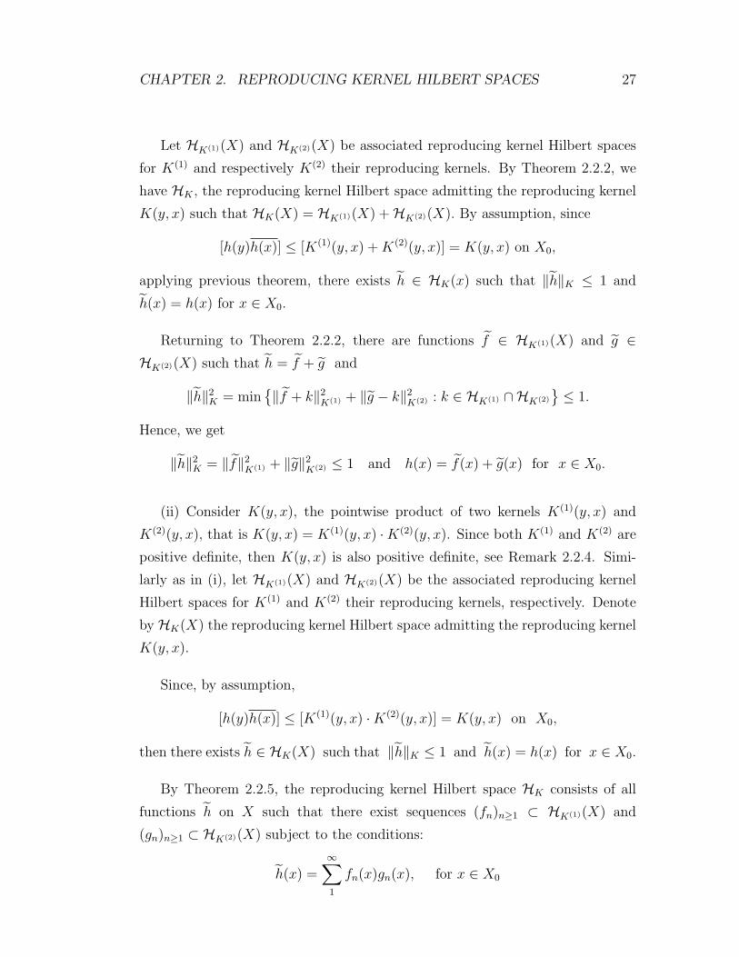
Let HK(1)(X) and HK(2)(X) be associated reproducing kernel Hilbert spaces
for K(1) and respectively K(2) their reproducing kernels. By Theorem 2.2.2, we
have HK , the reproducing kernel Hilbert space admitting the reproducing kernel
K(y, x) such that HK(X) = HK(1)(X) +HK(2)(X). By assumption, since
[h(y)h(x)] ≤ [K(1)(y, x) + K(2)(y, x)] = K(y, x) on X0,
applying previous theorem, there exists h ∈ HK(x) such that ‖h‖K ≤ 1 and
h(x) = h(x) for x ∈ X0.
Returning to Theorem 2.2.2, there are functions f ∈ HK(1)(X) and g ∈HK(2)(X) such that h = f + g and
‖h‖2K = min
‖f + k‖2K(1) + ‖g − k‖2
K(2) : k ∈ HK(1) ∩HK(2)
≤ 1.
Hence, we get
‖h‖2K = ‖f‖2
K(1) + ‖g‖2K(2) ≤ 1 and h(x) = f(x) + g(x) for x ∈ X0.
(ii) Consider K(y, x), the pointwise product of two kernels K(1)(y, x) and
K(2)(y, x), that is K(y, x) = K(1)(y, x) ·K(2)(y, x). Since both K(1) and K(2) are
positive definite, then K(y, x) is also positive definite, see Remark 2.2.4. Simi-
larly as in (i), let HK(1)(X) and HK(2)(X) be the associated reproducing kernel
Hilbert spaces for K(1) and K(2) their reproducing kernels, respectively. Denote
by HK(X) the reproducing kernel Hilbert space admitting the reproducing kernel
K(y, x).
Since, by assumption,
[h(y)h(x)] ≤ [K(1)(y, x) ·K(2)(y, x)] = K(y, x) on X0,
then there exists h ∈ HK(X) such that ‖h‖K ≤ 1 and h(x) = h(x) for x ∈ X0.
By Theorem 2.2.5, the reproducing kernel Hilbert space HK consists of all
functions h on X such that there exist sequences (fn)n≥1 ⊂ HK(1)(X) and
(gn)n≥1 ⊂ HK(2)(X) subject to the conditions:
h(x) =∞∑1
fn(x)gn(x), for x ∈ X0
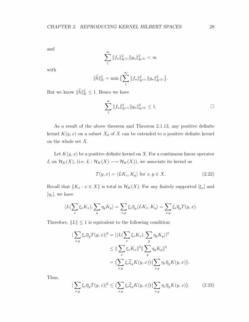
CHAPTER 2. REPRODUCING KERNEL HILBERT SPACES 28
and ∞∑1
‖fn‖2K(1)‖gn‖2
K(2) < ∞
with
‖h‖2K = min
∞∑1
‖fn‖2K(1)‖gn‖2
K(2)
.
But we know ‖h‖2K ≤ 1. Hence we have
∞∑1
‖fn‖2K(1)‖gn‖2
K(2) ≤ 1.
As a result of the above theorem and Theorem 2.1.13, any positive definite
kernel K(y, x) on a subset X0 of X can be extended to a positive definite kernel
on the whole set X.
Let K(y, x) be a positive definite kernel on X. For a continuous linear operator
L on HK(X), (i.e. L : HK(X) −→ HK(X)), we associate its kernel as
T (y, x) = 〈LKx, Ky〉 for x, y ∈ X. (2.22)
Recall that Kx : x ∈ X is total in HK(X). For any finitely supported [ξx] and
[ηx], we have
〈L(∑
x
ξxKx),∑
y
ηyKy〉 =∑x,y
ξxηy〈LKx, Ky〉 =∑x,y
ξxηyT (y, x).
Therefore, ‖L‖ ≤ 1 is equivalent to the following condition:
|∑x,y
ξxηyT (y, x)|2 = |〈L(∑
x
ξxKx),∑
y
ηyKy〉|2
≤ ‖∑
x
ξxKx‖2‖∑
y
ηyKy‖2
=(∑
x,y
ξxξyK(y, x))(∑
x,y
ηxηyK(y, x)).
Thus,
|∑x,y
ξxηyT (y, x)|2 ≤ (∑x,y
ξxξyK(y, x))(∑
x,y
ηxηyK(y, x)). (2.23)
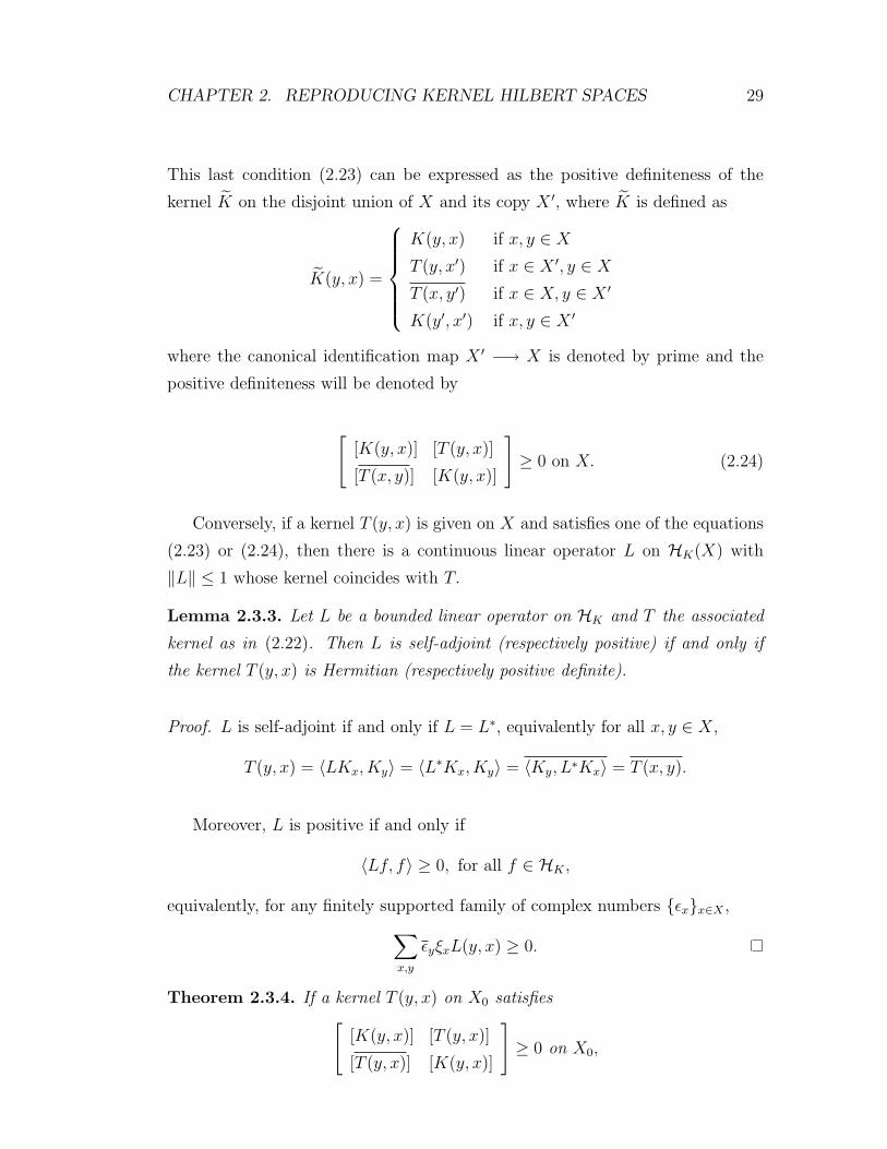
CHAPTER 2. REPRODUCING KERNEL HILBERT SPACES 29
This last condition (2.23) can be expressed as the positive definiteness of the
kernel K on the disjoint union of X and its copy X ′, where K is defined as
K(y, x) =
K(y, x) if x, y ∈ X
T (y, x′) if x ∈ X ′, y ∈ X
T (x, y′) if x ∈ X, y ∈ X ′
K(y′, x′) if x, y ∈ X ′
where the canonical identification map X ′ −→ X is denoted by prime and the
positive definiteness will be denoted by
[[K(y, x)] [T (y, x)]
[T (x, y)] [K(y, x)]
]≥ 0 on X. (2.24)
Conversely, if a kernel T (y, x) is given on X and satisfies one of the equations
(2.23) or (2.24), then there is a continuous linear operator L on HK(X) with
‖L‖ ≤ 1 whose kernel coincides with T.
Lemma 2.3.3. Let L be a bounded linear operator on HK and T the associated
kernel as in (2.22). Then L is self-adjoint (respectively positive) if and only if
the kernel T (y, x) is Hermitian (respectively positive definite).
Proof. L is self-adjoint if and only if L = L∗, equivalently for all x, y ∈ X,
T (y, x) = 〈LKx, Ky〉 = 〈L∗Kx, Ky〉 = 〈Ky, L∗Kx〉 = T (x, y).
Moreover, L is positive if and only if
〈Lf, f〉 ≥ 0, for all f ∈ HK ,
equivalently, for any finitely supported family of complex numbers εxx∈X ,
∑x,y
εyξxL(y, x) ≥ 0.
Theorem 2.3.4. If a kernel T (y, x) on X0 satisfies[
[K(y, x)] [T (y, x)]
[T (y, x)] [K(y, x)]
]≥ 0 on X0,
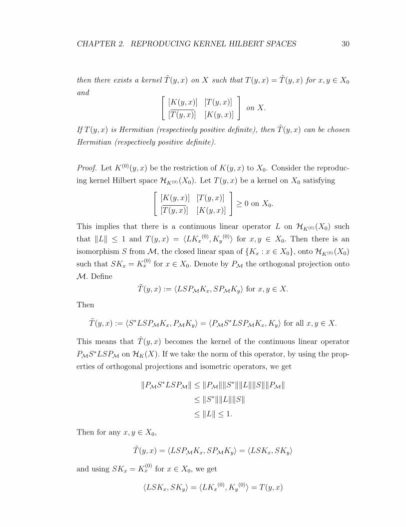
CHAPTER 2. REPRODUCING KERNEL HILBERT SPACES 30
then there exists a kernel T (y, x) on X such that T (y, x) = T (y, x) for x, y ∈ X0
and [[K(y, x)] [T (y, x)]
[T (y, x)] [K(y, x)]
]on X.
If T (y, x) is Hermitian (respectively positive definite), then T (y, x) can be chosen
Hermitian (respectively positive definite).
Proof. Let K(0)(y, x) be the restriction of K(y, x) to X0. Consider the reproduc-
ing kernel Hilbert space HK(0)(X0). Let T (y, x) be a kernel on X0 satisfying[
[K(y, x)] [T (y, x)]
[T (y, x)] [K(y, x)]
]≥ 0 on X0.
This implies that there is a continuous linear operator L on HK(0)(X0) such
that ‖L‖ ≤ 1 and T (y, x) = 〈LKx(0), Ky
(0)〉 for x, y ∈ X0. Then there is an
isomorphism S from M, the closed linear span of Kx : x ∈ X0, onto HK(0)(X0)
such that SKx = K(0)x for x ∈ X0. Denote by PM the orthogonal projection onto
M. Define
T (y, x) := 〈LSPMKx, SPMKy〉 for x, y ∈ X.
Then
T (y, x) := 〈S∗LSPMKx, PMKy〉 = 〈PMS∗LSPMKx, Ky〉 for all x, y ∈ X.
This means that T (y, x) becomes the kernel of the continuous linear operator
PMS∗LSPM on HK(X). If we take the norm of this operator, by using the prop-
erties of orthogonal projections and isometric operators, we get
‖PMS∗LSPM‖ ≤ ‖PM‖‖S∗‖‖L‖‖S‖‖PM‖≤ ‖S∗‖‖L‖‖S‖≤ ‖L‖ ≤ 1.
Then for any x, y ∈ X0,
T (y, x) = 〈LSPMKx, SPMKy〉 = 〈LSKx, SKy〉
and using SKx = K(0)x for x ∈ X0, we get
〈LSKx, SKy〉 = 〈LKx(0), Ky
(0)〉 = T (y, x)
CHAPTER 2. REPRODUCING KERNEL HILBERT SPACES 31
and hence
T (y, x) = T (y, x).
Moreover, if T (y, x) is Hermitian (respectively positive definite), then L∗ is
self-adjoint (respectively positive definite) by previous remark and so the op-
erator PMS∗LSPM will be self-adjoint (respectively positive definite). Denote
PMS∗LSPM = N. Then
T (y, x) = 〈PMS∗LSPMKx, Ky〉 = 〈NKx, Ky〉= 〈N∗Kx, Ky〉 = 〈Kx, NKy〉 = 〈NKy, Kx〉 = 〈T (x, y)〉.
So T (y, x) is Hermitian (respectively positive definite).
When L is self-adjoint, then ‖L‖ ≤ 1 if and only if
|〈Lf, f〉| ≤ ‖L‖‖f‖2K≤ ‖f‖2
K for all f ∈ HK(X). (2.25)
This implies
|〈L(∑
x
ξxKx),∑
y
ξyKy〉| ≤∑x,y
ξyξxK(y, x),
which is equivalent to
|∑x,y
ξyξxM(y, x)| ≤∑x,y
ξyξxK(y, x), for all [ξx]. (2.26)
When L is not self adjoint, then either of the equations (2.25) or equivalently
(2.26) only imply L ≤ 2.
Theorem 2.3.5. Let K(y, x) be a positive definite kernel on X, and let L(y, x) be
a kernel on X0. If for any finitely supported family of complex numbers ξxx∈X
|∑
x,y∈X0
ξyξxL(y, x)| ≤∑
x,y∈X0
ξyξxK(y, x), (2.27)
then there is a kernel L(y, x) on X such that L(y, x) = L(y, x) for all x, y ∈ X0
and
|∑x,y
ξyξxL(y, x)| ≤∑x,y
ξyξxK(y, x) for all [ξx].
If L(y, x) is Hermitian (respectively positive definite), L(y, x) can be chosen Her-
mitian (respectively positive definite).
CHAPTER 2. REPRODUCING KERNEL HILBERT SPACES 32
Proof. Let equation (2.27) be satisfied for K(y, x) a positive definite kernel on X
and let L(y, x) be a kernel on X0. So this is equivalent with Theorem 2.3.4. This
implies that the linear operator L on H(0)K (X0) satisfies
|〈Lh, h〉K(0) | ≤ ‖h‖2K(0) for h ∈ H(0)
K (X0).
Taking S isometric and choosing L(y, x) = 〈LSPMKx, SPMKy〉, similarly as in
the previous proof, we have
|〈LSPMf, SPMf〉K(0)| ≤ ‖SPMf‖2K(0) ≤ ‖f‖2
K for f ∈ HK(X).
Hence, similarly as in the previous proof, we find that L(y, x) = L(y, x) for
x, y ∈ X0. Therefore,
|∑x,y
ξyξxL(y, x)| = |∑x,y
ξyξx〈PMS∗LSPMKx, Ky〉|
= |〈PMS∗LSPM(∑
x
ξxKx),∑
y
ξyKy〉|
≤ ‖PMS∗LSPM‖‖∑
x
ξxKx‖2
≤∑x,y
ξyξx〈Kx, Ky〉
≤∑x,y
ξyξxK(y, x).
Chapter 3
Spaces of Analytic Functions
3.1 Sesqui-analytic kernels
Definition 3.1.1. A two variable function on a domain Ω in the complex plane,
is sesqui-analytic if it is analytic in the first variable and anti-analytic in the
second variable.
For example, this holds if the kernel K(w, z) is analytic in the first variable
and Hermitian, that is,
K(w, z) = Kz(w) = Kw(z) = K(z, w) for all w, z ∈ Ω.
Definition 3.1.2. A function f defined on some topological space X with real
or complex values is called locally bounded, if for any x0 in X, there exists a
neighborhood A of x0 such that f(A) is a bounded set, that is, for some number
M > 0, |f(x)| ≤ M for all x in A.
We have the kernel K(w, z) is locally bounded in the sense that it is bounded
on A×B for every pair A,B of compact subsets of a domain Ω.
Let us denote by Ω a connected domain of the complex plane.
33
CHAPTER 3. SPACES OF ANALYTIC FUNCTIONS 34
Theorem 3.1.3. The reproducing kernel Hilbert space HK(Ω) consists of analytic
functions on Ω if and only if the positive definite kernel K(w, z) on Ω is sesqui-
analytic and locally bounded.
Proof. Suppose that HK(Ω) consists of analytic functions on Ω. Let K(w, z) be
the reproducing kernel of HK(Ω) and note that Kz ∈ HK is analytic. By the
definition of a reproducing kernel which is positive definite, we have
K(w, z) = K(z, w) for all w, z ∈ Ω.
So K is sesqui-analytic. To see the localy boundedness, consider any pair A,Bof compact subsets of Ω. By assumption, every f ∈ HK(Ω) is analytic. Then
f(z) = 〈f,Kz〉, z ∈ Ω,
is analytic and hence continuous in z. Then the map z 7−→ Kz is weakly contin-
uous. This implies Kz : z ∈ A is weakly compact, thus weakly bounded. Then
by the Theorem A.3.6, weakly boundedness implies strong boundedness. That
is, supz∈A ‖Kz‖ =: γA < ∞. Now by Schwarz Inequality,
|K(w, z)| = |〈Kz, Kw〉| ≤ ‖Kz‖ · ‖Kw‖ ≤ γA · γB,
for w ∈ A, z ∈ B. Hence K is locally bounded.
Conversely, suppose that a positive definite kernel K(w, z) on Ω is sesqui-
analytic and locally bounded. Recall that the set Kz : z ∈ Ω is total in HK(Ω).
Then for each f ∈ HK(Ω), f is the strong limit of a sequence (fn)n≥1 in the
linear span of Kz : z ∈ Ω, that is ‖fn − f‖ −→ 0, as n →∞. By assumption,
since K(w, z) is sesqui-analytic, then K(w, z) = Kz(w) is analytic in w. Then by
reproducing property, since
fn(w) = 〈fn, Kw〉, w ∈ Ω,
it follows that fn is analytic. Since K(w, z) is locally bounded, we have
supz∈A ‖Kz‖ ≡ γA < ∞, where A is any compact subset of Ω. Then for w ∈ A,
|fn(w)− f(w)| = |〈fn, Kw〉 − 〈f, Kw〉| = |〈fn − f, Kw〉|= ‖fn − f‖‖Kw‖ ≤ γA‖fn − f‖
CHAPTER 3. SPACES OF ANALYTIC FUNCTIONS 35
and since ‖fn − f‖ −→ 0, (as n →∞), we have fn converges to f uniformly
on each compact subset A of Ω. Hence, HK(Ω) consists of analytic functions on
Ω.
Definition 3.1.4. A subset Λ of Ω is called determining subset if every analytic
function on Ω, equal to zero on Λ, vanishes identically on Ω. In particular, if Λ
has a limit point in Ω, it is a determining subset.
If two analytic functions are equal on a determining subset Λ, then they
coincide on the whole set Ω, i.e. f1|Λ = f2|Λ implies f1|Ω = f2|Ω.
In particular, given two sesqui-analytic kernels K(1)(w, z) and K(2)(w, z)
on Ω, if K(1)(w, z) = K(2)(w, z) for w, z ∈ Λ and Λ is determining subset, then
K(1)(w, z) = K(2)(w, z) on whole Ω.
Theorem 3.1.5. Let K(w, z) be a locally bounded, sesqui-analytic and positive
definite kernel on Ω and Λ a determining subset of Ω.
(i) If a function h on Λ satisfies the condition
[h(w)h(z)] ≤ [K(w, z)] on Λ, (3.1)
then there exists uniquely an analytic function h on Ω such that
h(z) = h(z) for z ∈ Λ and [h(w)h(z)] ≤ [K(w, z)]. (3.2)
(ii) If a positive definite kernel L(w, z) satisfies
[L(w, z)] ≤ [K(w, z)] on Λ, (3.3)
then there exists uniquely a sesqui-analytic positive definite kernel L(w, z) on Ω
such that
L(w, z) = L(w, z) for w, z ∈ Λ and [L(w, z)] ≤ [K(w, z)] on Ω. (3.4)
Proof. Let K(w, z) be a locally bounded, sequi-analytic and positive definite
kernel on Ω and Λ a determining subset of Ω.
CHAPTER 3. SPACES OF ANALYTIC FUNCTIONS 36
(i) Suppose that for a function h on Ω (3.1) is satisfied. Then by Theorem
2.3.1, there exists h ∈ HK(Ω) such that ‖h‖K ≤ 1 and h(z) = h(z) for z ∈ Λ.
By the same theorem, we can extend h(w)h(z) on Λ to a positive definite kernel
h(w)h(z) on Ω. Then h(w)h(z) = h(w)h(z) on Λ implies that
[h(w)h(z)] ≤ [K(w, z)].
Note that by Theorem 3.1.3, HK consists of analytic functions and hence h is
analytic as well. The uniqueness part follows due to the assumption on the set Λ
to be determining for Ω.
(ii) Suppose that a positive definite kernel L(y, x) satisfies the condition (3.3).
By Theorem 2.1.13 there exists a Hilbert space H and a function h : Λ → H such
that L(w, z) = 〈hz, hw〉H for all z, w ∈ Λ. Then we use part (i) for Hilbert space
valued functions.
In the successive theorem, we will use the following lemma:
Lemma 3.1.6. Let Ω be a domain in the complex plane and f either analytic
or harmonic in Ω. Then for all w ∈ Ω and ε > 0 such that D(w; ε) := z ∈ C :
|z − w| ≤ ε ⊂ Ω, we have
f(w) =1
πε2
∫∫
D(w;ε)
f(z)dm(z)
where m(·) is the planar Lebesque measure in C.
Proof. By writing f = u+ iv, it follows that it is sufficient to prove the statement
for f harmonic on Ω. Also recall that by the Cauchy integral formula for harmonic
functions, for all r ∈ [0, ε],
f(w) =1
2π
∫ 2π
0
f(w + reit)dt.
Then by using the change of variables to polar coordinates
x = a + r cos t, y = b + r sin t,
CHAPTER 3. SPACES OF ANALYTIC FUNCTIONS 37
where z = x + iy and w = a + ib, we have
1
πε2
∫∫
D(w,ε)
f(z)dm(z) =1
πε2
∫ ε
0
∫ 2π
0
f(w + reit)rdtdr
=1
πε2
∫ ε
0
( ∫ 2π
0
f(w + reit)dt)rdr
=1
πε2
∫ ε
0
2πf(w)rdr =2πf(w)
πε2· r2
2
∣∣∣ε
0
= f(w).
Theorem 3.1.7. Let K(w, z) be a locally bounded, sesqui-analytic kernel on Ω.
If K(w, z) is positive definite on a determining subset Λ, then it is on the whole
Ω.
Proof. Let K(w, z) be a locally bounded, sesqui-analytic kernel on Ω. Suppose
that K(w, z) is positive definite on Λ. Our aim is to show that K(w, z) is positive
definite on the whole Ω. The proof is divided in six steps:
Step 1: K(w, z) is Hermitian on Ω.
Since K(w, z) is positive definite on Λ, then K(w, z) = K(z, w) on Λ. Then
K(z, w) will also be sesqui-analytic on Λ. This implies that K(w, z) and K(z, w)
are equal on Ω. Hence K(w, z) is Hermitian.
Step 2: There exists a positive Borel function ρ(z) on Ω which satisfies the
following conditions:
(i) 1/ρ(z) is locally bounded.
(ii)∫Ω|K(w, z)|2ρ(z)dm(z) < ∞ for all w ∈ Ω.
(iii)∫Ω
∫Ω|K(w, z)|2ρ(z)ρ(w)dm(z)dm(w) < ∞
where m(·) denotes the planar Lebesque measure.
Let us write Ω as an increasing union of bounded subdomains Ωnn≥1 such
that Ωn ⊂ Ωn+1.
CHAPTER 3. SPACES OF ANALYTIC FUNCTIONS 38
Let supw,z∈Ωn|K(w, z)|2 = γn, (n = 1, 2, 3, . . .). Since K(w, z) is locally
bounded, we have γn < ∞ for each n.
We define ρ as follow,
ρ(z) :=1
2n(γn + 1)m(Ωn \ Ωn−1)for z ∈ Ωn \ Ωn−1 with Ω0 = ∅. (3.5)
(i) We have 1/ρ(z) is bounded on each Ωn and every compact subset of Ω is
absorbed in some Ωm. So we get 1/ρ(z) is locally bounded.
(ii) Let w ∈ Ωn \ Ωn−1. Then∫
Ω
|K(w, z)|2ρ(z)dm(z)
=∞∑
k=1
∫
Ωk\Ωk−1
|K(w, z)|2ρ(z)dm(z)
≤∞∑
k=1
∫
Ωk\Ωk−1
γkρ(z)dm(z)
=∞∑
k=1
∫
Ωk\Ωk−1
γk1
2k(γk + 1)m(Ωk \ Ωk−1)dm(z)
=∞∑
k=1
γk
2k(γk + 1)m(Ωk \ Ωk−1)
∫
Ωk\Ωk−1
dm(z)
≤∞∑
k=1
1/2k = 1 < ∞.
(iii) To see this we have the following estimations:∫
Ω
∫
Ω
|K(w, z)|2ρ(z)ρ(w)dm(z)dm(w)
=
∫
Ω
ρ(w)( ∫
Ω
|K(w, z)|2ρ(z)dm(z))dm(w)
=∞∑
k=1
∫
Ωk\Ωk−1
ρ(w)( ∫
Ω
|K(w, z)|2ρ(z)dm(z))dm(w)
≤∞∑
k=1
∫
Ωk\Ωk−1
ρ(w)dm(w) (by (ii))
=∞∑
k=1
1
2k(γk + 1)≤ 1 < ∞.
CHAPTER 3. SPACES OF ANALYTIC FUNCTIONS 39
Step 3: Define a new measure dµ(z) := ρ(z)dm(z) on Ω and let L2(Ω, µ) be
the associated Hilbert space. Let A2(Ω, µ) be the subspace of L2(Ω, µ) consisting
of all analytic functions in L2(Ω, µ). In the following we show that A2(Ω, µ) is a
reproducing kernel Hilbert space on Ω and it is closed in L2(Ω, µ).
Let us fix w ∈ Ω and take ε > 0 such that the open disk D(w, ε) := z :
|z−w| ≤ ε is contained in Ω. For any analytic function f ∈ A2(Ω, µ), according
to the previous lemma,
f(w) =1
πε2
∫
D(w,ε)
f(z)dm(z).
Then by the Schwarz Inequality in L2(Ω, µ),
|f(w)| =∣∣ 1
πε2
∫
D(w,ε)
f(z)dm(z)∣∣
=1
πε2
(∫
Ω
|f(z)|2ρ(z)dm(z))1/2( ∫
D(w,ε)
1/ρ(z)dm(z))1/2
≤ κ‖f‖
where κ is a finite constant depending on w and ε, but not on f ∈ A2(Ω, µ).
Thus, the point evaluation functional f 7−→ f(w) is continuous on L2(Ω, µ) and
hence A2(Ω, µ) is a reproducing kernel Hilbert space on Ω.
To see that A2(Ω, µ) is closed, by the above discussion, since |f(w)| ≤ κ‖f‖,the strong topology of A2(Ω, µ) is stronger then the topology of local uniform
convergence. This implies that the closure of A2(Ω, µ) consists of analytic func-
tions, that is, A2(Ω, µ) is closed in L2(Ω, µ).
Step 4: Define a linear operator K in L2(Ω, µ) such that
(Kf)(w) := 〈f, Kw〉 =
∫
Ω
K(w, z)f(z)dµ(z) (3.6)
for all f ∈ L2(Ω, µ) and w ∈ Ω. We claim that it is unique and bounded.
Note that by (ii), Kw(z) = K(z, w) = K(w, z) ∈ L2(Ω, µ) and hence K is
CHAPTER 3. SPACES OF ANALYTIC FUNCTIONS 40
well-defined. Then by using (iii) and (3.6),
∫
Ω
|(Kf)(w)|2dµ(w) =
∫
Ω
|〈f,Kw〉|2dµ(w)
≤∫
Ω
‖f‖2‖Kw‖2dµ(w)
= ‖f‖2
∫
Ω
〈Kw, Kw〉dµ(w)
= ‖f‖2
∫
Ω
K(w, z)Kw(z)ρ(z)dm(z)ρ(w)dm(w)
= ‖f‖2
∫
Ω
∫
Ω
|K(w, z)|2ρ(z)ρ(w)dm(z)dm(w)
≤ C‖f‖2
where C is a finite constant. Hence K is bounded.
Step 5 : K maps L2(Ω, µ) in A2(Ω, µ).
Note that since the kernel K is Hermitian, it follows that the operator K
is self-adjoint. Since A2(Ω, µ) is a closed subspace and all analytic functions in
L2(Ω, µ) are contained in A2(Ω, µ) and for all w, Kw(z) is analytic in z, it follows
that Kw ∈ A2(Ω, µ). By Step 4, we have
Kw : w ∈ Ω⊥ ⊆ ker(K) = (RanK∗)⊥ = (RanK)⊥, as K = K∗.
Then (RanK) = (RanK∗) ⊂ A2(Ω, µ).
Step 6: Let L(w, z) be the reproducing kernel of A2(Ω, µ). Then we have
〈KLz, Lw〉 = K(w, z) for all w, z ∈ Ω.
Let P be the orthogonal projection onto A2(Ω, µ). Then for f ∈ L2(Ω, µ), we
have 〈Kf, f〉 = 〈KPf, Pf〉 since RanK ⊂ A2(Ω, µ) and K is self adjoint.
In Step 4, put Lz instead of f with the reproducing property,
(KLz)(u) = 〈Lz, Ku〉 = Ku(z) = K(z, u) = K(u, z) = Kz(u) (3.7)
and
〈KLz, Lw〉 = 〈Kz, Lw〉 = 〈Lw, Kz〉 = Kw(z) = Kz(w) = K(w, z) (3.8)
CHAPTER 3. SPACES OF ANALYTIC FUNCTIONS 41
for w, z ∈ Ω.
Since Λ is a determining subset of Ω and Lz : z ∈ Ω is total in A2(Ω, µ), it
follows that Lz : z ∈ Λ is total in A2(Ω, µ). Therefore, by (3.8) and taking into
account that the linear operator K is bounded and that the kernel K is positive
on Λ, it follows that the operator K is positive and hence the kernel K is positive
definite on Ω.
Theorem 3.1.8. Suppose that Ω(1) ∩Ω(2) 6= ∅ where Ω(1) and Ω(2) are connected
domains of the complex plane. If K(1)(w, z) and K(2)(w, z) are locally bounded,
sesqui-analytic, positive definite kernels on Ω(1) and Ω(2) respectively, such that
K(1)(w, z) = K(2)(w, z) for all w, z ∈ Ω(1) ∩ Ω(2), (3.9)
then there exists uniquely a locally bounded, sesqui-analytic, positive definite ker-
nel K(w, z) on Ω(1) ∪ Ω(2) such that
K(w, z) = K(i)(w, z) for w, z ∈ Ω(i), (i = 1, 2). (3.10)
Proof. Let Ω be the intersection of Ω(1) and Ω(2) and K(w, z) be the restriction
of K(1)(w, z) = K(2)(w, z) to this Ω for w, z ∈ Ω. So we have
K(w, z) = K(1)(w, z) = K(2)(w, z) for w, z ∈ Ω.
Since Ω is open in connected Ω(i), Ω is a determining subset of Ω(1) and Ω(2).
Then, there exists an isometric operator T (i) from HK(i)(Ω(i)) to HK(Ω) such that
T (i)K(i)z = Kz for z ∈ Ω (i = 1, 2).
Now we can define the kernel K(w, z) on Ω := Ω(1) ∪ Ω(2) by
K(w, z) := 〈T (i)K(i)z , T (j)K(j)
w 〉K if w ∈ Ω(i), z ∈ Ω(j) and i, j ∈ 1, 2.
Then, since K(1)(w, z) and K(2)(w, z) are locally bounded and sesqui-analytic, so
is K(w, z).
Moreover by the isometric property of operator T (i), we get from the last
equation that
K(w, z) = K(i)(w, z) for w, z ∈ Ω(i) (i = 1, 2).
CHAPTER 3. SPACES OF ANALYTIC FUNCTIONS 42
Finally, since K(w, z) is locally bounded and sesqui-analytic on Ω, and K(w, z)
is positive definite on the determining subset Ω of Ω, by Theorem 3.1.7, K(w, z)
is positive definite on the whole Ω.
3.2 Bergman Spaces
Definition 3.2.1. The space of all analytic functions f(z) on Ω for which∫∫
Ω
|f(z)|2dxdy < ∞, (z = x + iy)
is satisfied, is called the Bergman space on Ω and denoted by A2(Ω).
Remark 3.2.2. A2(Ω) is a reproducing kernel Hilbert space with respect to the
inner product
〈f, g〉 ≡ 〈f, g〉Ω :=
∫
Ω
∫f(z)g(z)dxdy
and its kernel is called the Bergman kernel of Ω and denoted by B(Ω)(w, z).
In the following we will calculate the Bergman kernel for any simply connected
domain Ω. Consider the simplest case, that is Ω = D, where D := z : |z| < 1.For this case the inner product is
〈f, g〉 =
∫ 1
0
∫ 2π
0
f(reiθ)g(reiθ)dθrdr, (z = reiθ, r ≤ 1).
Theorem 3.2.3. The Bergman kernel for the open unit disc D is given by
B(D)(w, z) =1
π
1
(1− wz)2for w, z ∈ D. (3.11)
Proof. We divide the proof in three steps.
Step 1: fn(z) =√
n+1π
zn, (n=0,1,2,. . . ) form an orthonormal sequence in
A2(D).
Since
〈zn, zm〉 =
∫ 1
0
∫ 2π
0
rneinθrme−imθdθrdr =2π
n + m + 2δnm,
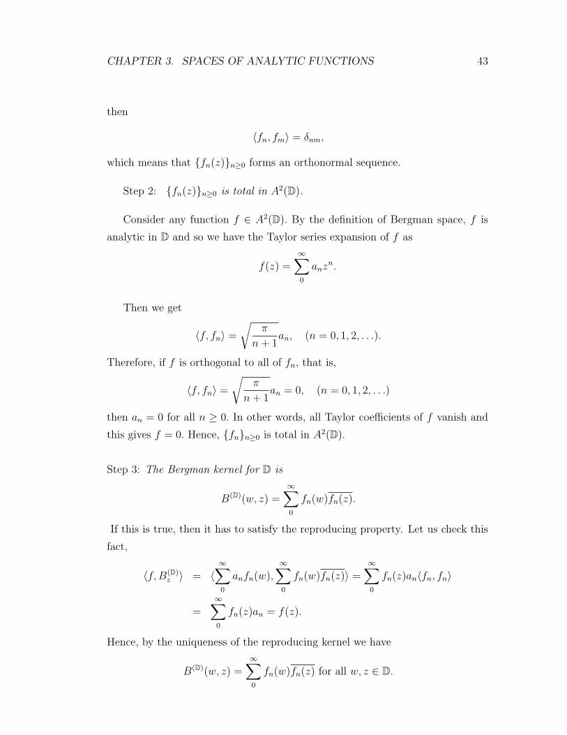
CHAPTER 3. SPACES OF ANALYTIC FUNCTIONS 43
then
〈fn, fm〉 = δnm,
which means that fn(z)n≥0 forms an orthonormal sequence.
Step 2: fn(z)n≥0 is total in A2(D).
Consider any function f ∈ A2(D). By the definition of Bergman space, f is
analytic in D and so we have the Taylor series expansion of f as
f(z) =∞∑0
anzn.
Then we get
〈f, fn〉 =
√π
n + 1an, (n = 0, 1, 2, . . .).
Therefore, if f is orthogonal to all of fn, that is,
〈f, fn〉 =
√π
n + 1an = 0, (n = 0, 1, 2, . . .)
then an = 0 for all n ≥ 0. In other words, all Taylor coefficients of f vanish and
this gives f = 0. Hence, fnn≥0 is total in A2(D).
Step 3: The Bergman kernel for D is
B(D)(w, z) =∞∑0
fn(w)fn(z).
If this is true, then it has to satisfy the reproducing property. Let us check this
fact,
〈f,B(D)z 〉 = 〈
∞∑0
anfn(w),∞∑0
fn(w)fn(z)〉 =∞∑0
fn(z)an〈fn, fn〉
=∞∑0
fn(z)an = f(z).
Hence, by the uniqueness of the reproducing kernel we have
B(D)(w, z) =∞∑0
fn(w)fn(z) for all w, z ∈ D.
CHAPTER 3. SPACES OF ANALYTIC FUNCTIONS 44
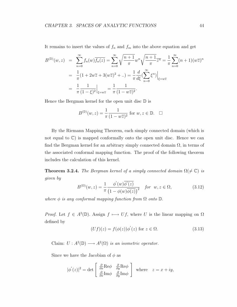
It remains to insert the values of fn and fm into the above equation and get
B(D)(w, z) =∞∑
n=0
fn(w)fn(z) =∞∑
n=0
√n + 1
πwn
√n + 1
πzn =
1
π
∞∑n=0
(n + 1)(wz)n
=1
π(1 + 2wz + 3(wz)2 + ..) =
1
π
d
dξ(∞∑
n=0
ξn)∣∣∣ξ=wz
=1
π
1
(1− ξ)2
∣∣∣ξ=wz
=1
π
1
(1− wz)2.
Hence the Bergman kernel for the open unit disc D is
B(D)(w, z) =1
π
1
(1− wz)2for w, z ∈ D.
By the Riemann Mapping Theorem, each simply connected domain (which is
not equal to C) is mapped conformally onto the open unit disc. Hence we can
find the Bergman kernel for an arbitrary simply connected domain Ω, in terms of
the associated conformal mapping function. The proof of the following theorem
includes the calculation of this kernel.
Theorem 3.2.4. The Bergman kernel of a simply connected domain Ω(6= C) is
given by
B(Ω)(w, z) =1
π
φ′(w)φ′(z)(
1− φ(w)φ(z))2 for w, z ∈ Ω, (3.12)
where φ is any conformal mapping function from Ω onto D.
Proof. Let f ∈ A2(D). Assign f 7−→ Uf, where U is the linear mapping on Ω
defined by
(Uf)(z) = f(φ(z))φ′(z) for z ∈ Ω. (3.13)
Claim: U : A2(D) −→ A2(Ω) is an isometric operator.
Since we have the Jacobian of φ as
|φ′(z)|2 = det
[∂∂x
Reφ ∂∂y
Reφ∂∂x
Imφ ∂∂y
Imφ
]where z = x + iy,
CHAPTER 3. SPACES OF ANALYTIC FUNCTIONS 45
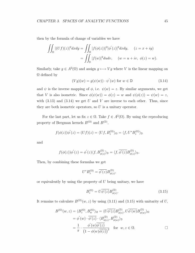
then by the formula of change of variables we have∫∫
Ω
|(Uf)(z)|2dxdy =
∫∫
Ω
|f(φ(z))|2|φ′(z)|2dxdy, (z = x + iy)
=
∫∫
D|f(w)|2dudv, (w = u + iv, φ(z) = w).
Similarly, take g ∈ A2(Ω) and assign g 7−→ V g where V is the linear mapping on
Ω defined by
(V g)(w) = g(ψ(w)) · ψ′(w) for w ∈ D (3.14)
and ψ is the inverse mapping of φ, i.e. ψ(w) = z. By similar arguments, we get
that V is also isometric. Since φ(ψ(w)) = φ(z) = w and ψ(φ(z)) = ψ(w) = z,
with (3.13) and (3.14) we get U and V are inverse to each other. Thus, since
they are both isometric operators, so U is a unitary operator.
For the last part, let us fix z ∈ Ω. Take f ∈ A2(Ω). By using the reproducing
property of Bergman kernels B(Ω) and B(D),
f(φ(z))φ′(z) = (Uf)(z) = 〈Uf,B(Ω)
z 〉Ω = 〈f, U∗B(Ω)z 〉D
and
f(φ(z))φ′(z) = φ
′(z)〈f, B
(D)φ(z)〉D = 〈f, φ′(z)B
(D)φ(z)〉D.
Then, by combining these formulas we get
U∗B(Ω)z = φ′(z)B
(D)φ(z),
or equivalently by using the property of U being unitary, we have
B(Ω)z = Uφ′(z)B
(D)φ(z). (3.15)
It remains to calculate B(Ω)(w, z) by using (3.11) and (3.15) with unitarity of U,
B(Ω)(w, z) = 〈B(Ω)z , B(Ω)
w 〉Ω = 〈Uφ′(z)B(D)φ(z), Uφ′(w)B
(D)φ(w)〉Ω
= φ′(w) · φ′(z) · 〈B(D)
φ(z), B(D)φ(w)〉D
=1
π· φ
′(w)φ′(z)(
1− φ(w)φ(z))2 for w, z ∈ Ω.
CHAPTER 3. SPACES OF ANALYTIC FUNCTIONS 46
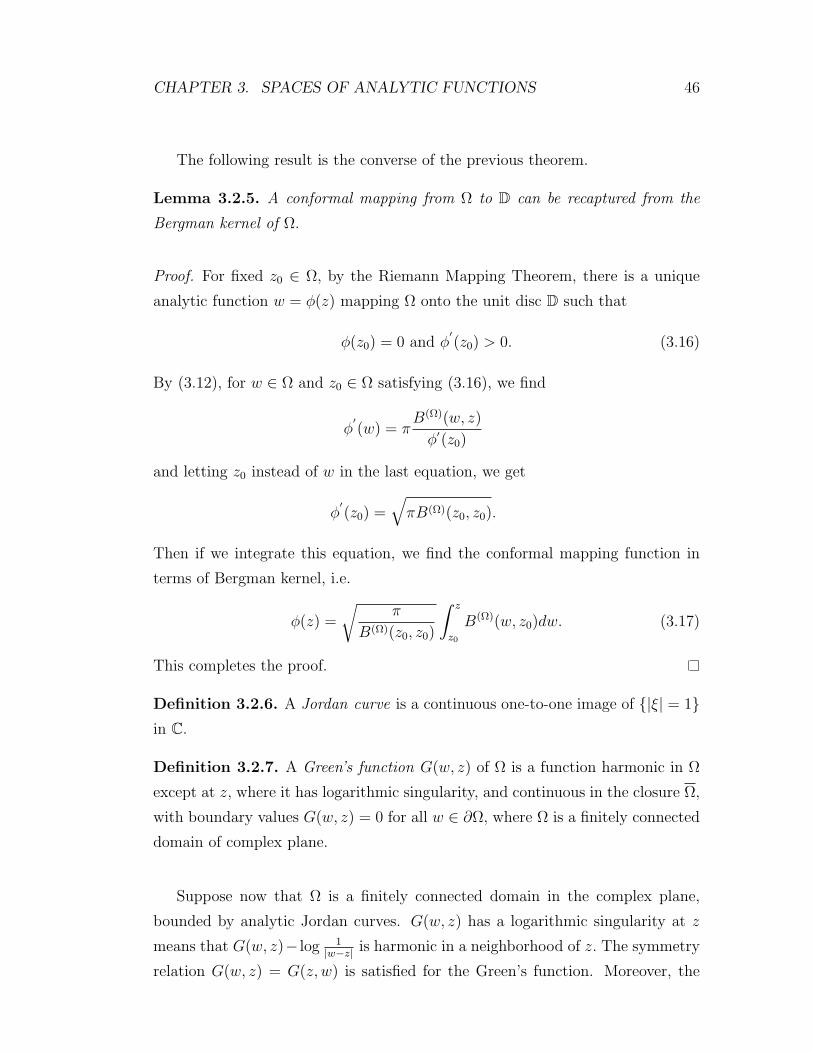
The following result is the converse of the previous theorem.
Lemma 3.2.5. A conformal mapping from Ω to D can be recaptured from the
Bergman kernel of Ω.
Proof. For fixed z0 ∈ Ω, by the Riemann Mapping Theorem, there is a unique
analytic function w = φ(z) mapping Ω onto the unit disc D such that
φ(z0) = 0 and φ′(z0) > 0. (3.16)
By (3.12), for w ∈ Ω and z0 ∈ Ω satisfying (3.16), we find
φ′(w) = π
B(Ω)(w, z)
φ′(z0)
and letting z0 instead of w in the last equation, we get
φ′(z0) =
√πB(Ω)(z0, z0).
Then if we integrate this equation, we find the conformal mapping function in
terms of Bergman kernel, i.e.
φ(z) =
√π
B(Ω)(z0, z0)
∫ z
z0
B(Ω)(w, z0)dw. (3.17)
This completes the proof.
Definition 3.2.6. A Jordan curve is a continuous one-to-one image of |ξ| = 1in C.
Definition 3.2.7. A Green’s function G(w, z) of Ω is a function harmonic in Ω
except at z, where it has logarithmic singularity, and continuous in the closure Ω,
with boundary values G(w, z) = 0 for all w ∈ ∂Ω, where Ω is a finitely connected
domain of complex plane.
Suppose now that Ω is a finitely connected domain in the complex plane,
bounded by analytic Jordan curves. G(w, z) has a logarithmic singularity at z
means that G(w, z)− log 1|w−z| is harmonic in a neighborhood of z. The symmetry
relation G(w, z) = G(z, w) is satisfied for the Green’s function. Moreover, the
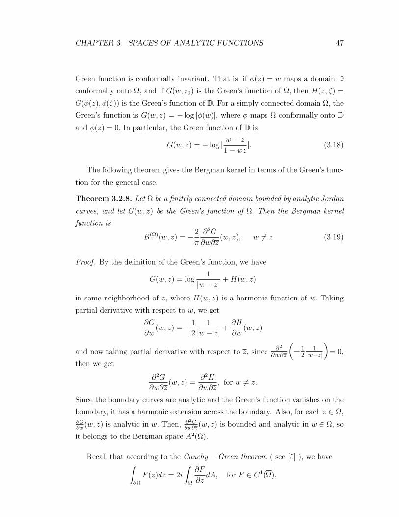
CHAPTER 3. SPACES OF ANALYTIC FUNCTIONS 47
Green function is conformally invariant. That is, if φ(z) = w maps a domain Dconformally onto Ω, and if G(w, z0) is the Green’s function of Ω, then H(z, ζ) =
G(φ(z), φ(ζ)) is the Green’s function of D. For a simply connected domain Ω, the
Green’s function is G(w, z) = − log |φ(w)|, where φ maps Ω conformally onto Dand φ(z) = 0. In particular, the Green function of D is
G(w, z) = − log | w − z
1− wz|. (3.18)
The following theorem gives the Bergman kernel in terms of the Green’s func-
tion for the general case.
Theorem 3.2.8. Let Ω be a finitely connected domain bounded by analytic Jordan
curves, and let G(w, z) be the Green’s function of Ω. Then the Bergman kernel
function is
B(Ω)(w, z) = − 2
π
∂2G
∂w∂z(w, z), w 6= z. (3.19)
Proof. By the definition of the Green’s function, we have
G(w, z) = log1
|w − z| + H(w, z)
in some neighborhood of z, where H(w, z) is a harmonic function of w. Taking
partial derivative with respect to w, we get
∂G
∂w(w, z) = −1
2
1
|w − z| +∂H
∂w(w, z)
and now taking partial derivative with respect to z, since ∂2
∂w∂z
(−1
21
|w−z|)
= 0,
then we get
∂2G
∂w∂z(w, z) =
∂2H
∂w∂z, for w 6= z.
Since the boundary curves are analytic and the Green’s function vanishes on the
boundary, it has a harmonic extension across the boundary. Also, for each z ∈ Ω,∂G∂w
(w, z) is analytic in w. Then, ∂2G∂w∂z
(w, z) is bounded and analytic in w ∈ Ω, so
it belongs to the Bergman space A2(Ω).
Recall that according to the Cauchy −Green theorem ( see [5] ), we have∫
∂Ω
F (z)dz = 2i
∫
Ω
∂F
∂zdA, for F ∈ C1(Ω).
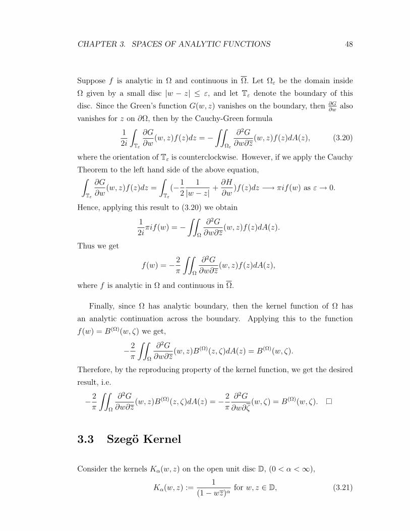
CHAPTER 3. SPACES OF ANALYTIC FUNCTIONS 48
Suppose f is analytic in Ω and continuous in Ω. Let Ωε be the domain inside
Ω given by a small disc |w − z| ≤ ε, and let Tε denote the boundary of this
disc. Since the Green’s function G(w, z) vanishes on the boundary, then ∂G∂w
also
vanishes for z on ∂Ω, then by the Cauchy-Green formula
1
2i
∫
Tε
∂G
∂w(w, z)f(z)dz = −
∫∫
Ωε
∂2G
∂w∂z(w, z)f(z)dA(z), (3.20)
where the orientation of Tε is counterclockwise. However, if we apply the Cauchy
Theorem to the left hand side of the above equation,∫
Tε
∂G
∂w(w, z)f(z)dz =
∫
Tε
(−1
2
1
|w − z| +∂H
∂w)f(z)dz −→ πif(w) as ε → 0.
Hence, applying this result to (3.20) we obtain
1
2iπif(w) = −
∫∫
Ω
∂2G
∂w∂z(w, z)f(z)dA(z).
Thus we get
f(w) = − 2
π
∫∫
Ω
∂2G
∂w∂z(w, z)f(z)dA(z),
where f is analytic in Ω and continuous in Ω.
Finally, since Ω has analytic boundary, then the kernel function of Ω has
an analytic continuation across the boundary. Applying this to the function
f(w) = B(Ω)(w, ζ) we get,
− 2
π
∫∫
Ω
∂2G
∂w∂z(w, z)B(Ω)(z, ζ)dA(z) = B(Ω)(w, ζ).
Therefore, by the reproducing property of the kernel function, we get the desired
result, i.e.
− 2
π
∫∫
Ω
∂2G
∂w∂z(w, z)B(Ω)(z, ζ)dA(z) = − 2
π
∂2G
∂w∂ζ(w, ζ) = B(Ω)(w, ζ).
3.3 Szego Kernel
Consider the kernels Kα(w, z) on the open unit disc D, (0 < α < ∞),
Kα(w, z) :=1
(1− wz)αfor w, z ∈ D, (3.21)
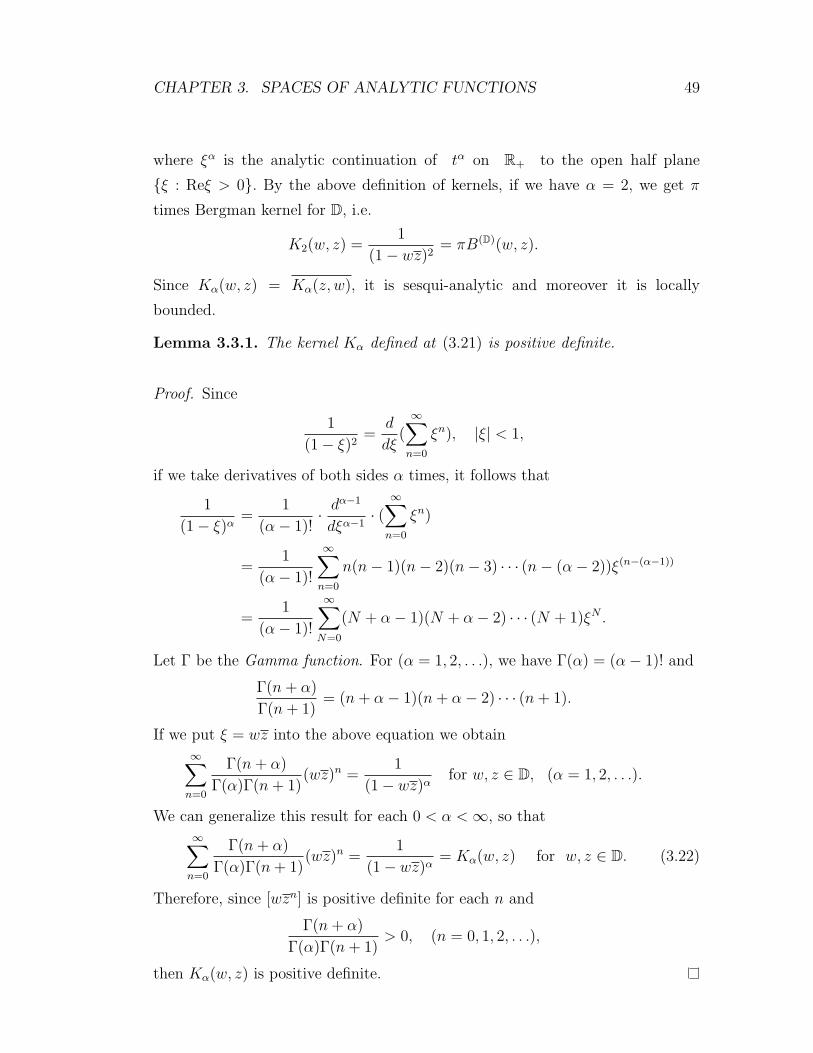
CHAPTER 3. SPACES OF ANALYTIC FUNCTIONS 49
where ξα is the analytic continuation of tα on R+ to the open half plane
ξ : Reξ > 0. By the above definition of kernels, if we have α = 2, we get π
times Bergman kernel for D, i.e.
K2(w, z) =1
(1− wz)2= πB(D)(w, z).
Since Kα(w, z) = Kα(z, w), it is sesqui-analytic and moreover it is locally
bounded.
Lemma 3.3.1. The kernel Kα defined at (3.21) is positive definite.
Proof. Since
1
(1− ξ)2=
d
dξ(∞∑
n=0
ξn), |ξ| < 1,
if we take derivatives of both sides α times, it follows that
1
(1− ξ)α=
1
(α− 1)!· dα−1
dξα−1· (
∞∑n=0
ξn)
=1
(α− 1)!
∞∑n=0
n(n− 1)(n− 2)(n− 3) · · · (n− (α− 2))ξ(n−(α−1))
=1
(α− 1)!
∞∑N=0
(N + α− 1)(N + α− 2) · · · (N + 1)ξN .
Let Γ be the Gamma function. For (α = 1, 2, . . .), we have Γ(α) = (α− 1)! and
Γ(n + α)
Γ(n + 1)= (n + α− 1)(n + α− 2) · · · (n + 1).
If we put ξ = wz into the above equation we obtain
∞∑n=0
Γ(n + α)
Γ(α)Γ(n + 1)(wz)n =
1
(1− wz)αfor w, z ∈ D, (α = 1, 2, . . .).
We can generalize this result for each 0 < α < ∞, so that
∞∑n=0
Γ(n + α)
Γ(α)Γ(n + 1)(wz)n =
1
(1− wz)α= Kα(w, z) for w, z ∈ D. (3.22)
Therefore, since [wzn] is positive definite for each n and
Γ(n + α)
Γ(α)Γ(n + 1)> 0, (n = 0, 1, 2, . . .),
then Kα(w, z) is positive definite.
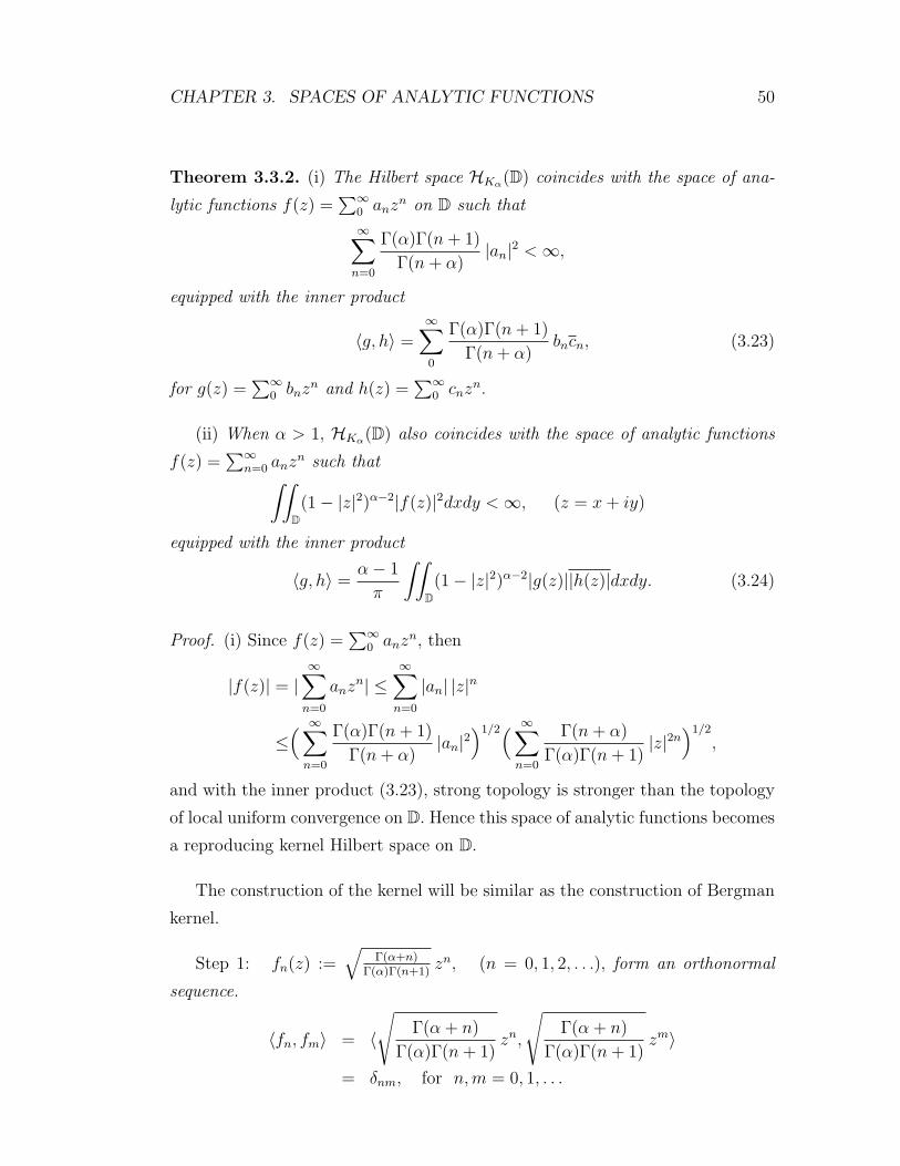
CHAPTER 3. SPACES OF ANALYTIC FUNCTIONS 50
Theorem 3.3.2. (i) The Hilbert space HKα(D) coincides with the space of ana-
lytic functions f(z) =∑∞
0 anzn on D such that
∞∑n=0
Γ(α)Γ(n + 1)
Γ(n + α)|an|2 < ∞,
equipped with the inner product
〈g, h〉 =∞∑0
Γ(α)Γ(n + 1)
Γ(n + α)bncn, (3.23)
for g(z) =∑∞
0 bnzn and h(z) =
∑∞0 cnz
n.
(ii) When α > 1, HKα(D) also coincides with the space of analytic functions
f(z) =∑∞
n=0 anzn such that
∫∫
D(1− |z|2)α−2|f(z)|2dxdy < ∞, (z = x + iy)
equipped with the inner product
〈g, h〉 =α− 1
π
∫∫
D(1− |z|2)α−2|g(z)||h(z)|dxdy. (3.24)
Proof. (i) Since f(z) =∑∞
0 anzn, then
|f(z)| = |∞∑
n=0
anzn| ≤
∞∑n=0
|an| |z|n
≤( ∞∑
n=0
Γ(α)Γ(n + 1)
Γ(n + α)|an|2
)1/2( ∞∑n=0
Γ(n + α)
Γ(α)Γ(n + 1)|z|2n
)1/2
,
and with the inner product (3.23), strong topology is stronger than the topology
of local uniform convergence on D. Hence this space of analytic functions becomes
a reproducing kernel Hilbert space on D.
The construction of the kernel will be similar as the construction of Bergman
kernel.
Step 1: fn(z) :=√
Γ(α+n)Γ(α)Γ(n+1)
zn, (n = 0, 1, 2, . . .), form an orthonormal
sequence.
〈fn, fm〉 = 〈√
Γ(α + n)
Γ(α)Γ(n + 1)zn,
√Γ(α + n)
Γ(α)Γ(n + 1)zm〉
= δnm, for n,m = 0, 1, . . .
CHAPTER 3. SPACES OF ANALYTIC FUNCTIONS 51
Thus, fnn≥0 is an orthonormal sequence.
Step 2: fnn≥0 is complete.
Consider the inner product in (3.23) of fn(z) with f =∑∞
n=0 akzk,
〈f, fn〉 = an
√Γ(α)Γ(n + 1)
Γ(n + α), (n = 0, 1, 2, . . .).
Therefore, f is orthogonal to all of fn, that is
〈f, fn〉 = an
√Γ(α)Γ(n + 1)
Γ(n + α)= 0, (n = 0, 1, 2, . . .)
only if an = 0 for each n. Thus f = 0 and fn is total.
Step 3: Kα(w, z) =∑∞
n=0 fn(w)fn(z).
To prove this, we verify the reproducing property:
〈f,Kz〉 = 〈∞∑
n=0
anfn(w),∞∑
n=0
fn(w)fn(z)〉
=∞∑
n=0
anfn(z) = f(z).
Hence, Kα(w, z) =∑∞
n=0 fn(w)fn(z).
Finally, inserting the values of fn(w) and fn(z) in this equation, we get
Kα(w, z) =∞∑
n=0
fn(w)fn(z) =∞∑
n=0
√Γ(α + n)
Γ(α)Γ(n + 1)wn
√Γ(α + n)
Γ(α)Γ(n + 1)zn
=∞∑
n=0
Γ(α + n)
Γ(α)Γ(n + 1)(wz)n =
1
(1− wz)α.
(ii) We change the coordinates to polar coordinates. For f =∑∞
n=0 anzn,
CHAPTER 3. SPACES OF ANALYTIC FUNCTIONS 52
consider the following integration,
α− 1
π
∫∫
D(1− |z|2)α−2|f(z)|2dxdy
=α− 1
π
∫ 1
0
∫ 2π
0
(1− r2)α−2|∞∑
n=0
an(reiθ)n|2dθrdr (z = reiθ)
=α− 1
π
∫ 1
0
∫ 2π
0
(1− r2)α−2( ∑
n,m≥0
amanrmrmeiθ(m−n))dθrdr
=α− 1
π
∑n,m≥0
aman
∫ 1
0
∫ 2π
0
(1− r2)α−2 rm+n+1eiθ(m−n)dθdr
=α− 1
π
∞∑n=0
|an|2∫ 1
0
2π(1− r2)α−2r2n+1dθdr
= 2(α− 1)∞∑
n=0
|an|2∫ 1
0
2π(1− r2)α−2r2n+1dθdr (t = r2, dt = 2rdr)
= (α− 1)∞∑
n=0
|an|2∫ 1
0
(1− t)α−2tndt.
Since∫ 1
0
(1− t)β−1tγ−1dt =Γ(β)Γ(γ)
Γ(β + γ), for β, γ > 0,
then
(α− 1)
∫ 1
0
(1− t)α−2tndt = (α− 1)Γ(α− 1)Γ(n + 1)
Γ(n + α)=
Γ(α)Γ(n + 1)
Γ(n + α).
Inserting this in the above integration, we get
(α− 1)∞∑0
|an|2∫ 1
0
(1− t)α−2tndt =∞∑0
Γ(α)Γ(n + 1)
Γ(n + α)|an|2
or equivalently,
α− 1
π
∫∫
D(1− |z|2)α−2|f(z)|2dxdy =
∞∑0
Γ(α)Γ(n + 1)
Γ(n + α)|an|2.
Hence, the last equality shows that on the space of analytic functions, the two
inner products (3.23) and (3.24) are the same.
CHAPTER 3. SPACES OF ANALYTIC FUNCTIONS 53
According to the values that α takes, the behavior of HKα(D) changes. If
α > 1, HKα(D) becomes a Hilbert space of analytic functions f(z) on D such
that∫
D|f(z)|2dµα(z) < ∞,
where µα is the measure on D given by
dµα(z) =α− 1
π(1− |z|2)α−2dxdy, (z = x + iy).
Definition 3.3.3. For α > 1, HKα(D) is called the weighted Bergman space on
D (with weight α−1π
(1− |z|2)α−2).
Lemma 3.3.4. If α < 1, HKα(D) is not a reproducing kernel Hilbert space with
respect to the inner product (3.24).
Proof. Suppose that for α < 1, HKα(D) is a reproducing kernel space. Let φ(z)
be an analytic function such that |φ(z)| ≤ 1 for z ∈ D. Then f 7−→ φ · f defines
a continuous linear operator on HKα(D) such that
‖φ f‖Kα ≤ ‖f‖Kα , where f ∈ HKα(D). (3.25)
Then, in terms of the kernel Kα(w, z), inequality (3.25) becomes
[φ(w) Kα(w, z) φ(z)] ≤ [Kα(w, z)] on D,
and hence we get
[Kα(w, z)(1− φ(w) φ(z))] ≥ 0 on D.
This implies that, for any z ∈ D, the following 2× 2 matrix is positive definite
[Kα(0, 0)(1− |φ(0)|2) Kα(0, z)(1− φ(0)φ(z))
Kα(z, 0)(1− φ(z)φ(0)) Kα(z, z)(1− |φ(z)|2)
]≥ 0. (3.26)
If φ(0) = 0, then (3.26) becomes
[Kα(0, 0) Kα(0, z)
Kα(z, 0) Kα(z, z)(1− |φ(z)|2)
]=
[1 1
1 1(1−|z|2)α (1− |φ(z)|2)
]≥ 0,
CHAPTER 3. SPACES OF ANALYTIC FUNCTIONS 54
where Kα(w, z) = 1/(1− wz)α. This implies
1− |φ(z)|2(1− |z|2)α
− 1 ≥ 0 and 1− (1− |z|2)α ≥ |φ(z)|2.
Then, for 0 6= z ∈ D,1− (1− |z|2)α
|z|2 ≥ |φ(z)|2|z|2 . (3.27)
Now consider the analytic function φt(z) := z(z − t)/(1− tz), (0 < t < 1), which
satisfies φt(0) = 0 and |φt(z)| ≤ 1 for z ∈ D and fix z0 ∈ D. Since we have α < 1,
then
(1− |z0|2)α > 1− |z0|2
and by this, we get the following
1 >1− (1− |z0|2)α
|z0|2 . (3.28)
Then, if we take the limit of |φt(z0)/z0|2 as t −→ 1,
limt→1
|φt(z0)/z0|2 = limt→1
∣∣∣ z0(z0 − t)
(1− tz0)z0
∣∣∣2
= limt→1
∣∣∣ z0 − t
1− tz0
∣∣∣2
= 1.
But this contradicts with the inequality (3.27). Hence, for α < 1, HKα(D) is not
a reproducing kernel Hilbert space with respect to the inner product (3.24).
It remains the case when α = 1. Let us denote by T the boundary of D, i.e.
T = ξ : |ξ| = 1 and let σ be the normalized arc-length measure such that
dσ(ξ) :=1
2π|dξ| ≡ 1
2πdθ, (ξ = eiθ).
Consider the Hilbert space L2(T) ≡ L2(T, σ) of measurable functions on T. We
have the inner product
〈f, g〉L2 :=
∫
Tf(ξ)g(ξ)dσ(ξ),
with respect to which the functions φn(ξ) := ξn, (n ∈ Z), which form a complete
orthonormal sequence.
Definition 3.3.5. The closed linear span of φn : n = 0, 1, · · · is called the
Hardy space on T and is denoted by H2(T).
CHAPTER 3. SPACES OF ANALYTIC FUNCTIONS 55
By Corollary A.2.3, f ∈ L2(T) belongs to Hardy space H2(T) if and only if
it is orthonormal to all φn (n < 0,) i.e. all Fourier coefficients of f which have
negative indices vanish. Then we have
〈f, g〉L2 =∞∑
n=0
anbn for f, g ∈ H2(T), (3.29)
where
an = 〈f, φn〉L2 and bn = 〈g, φn〉L2 (n = 0, 1, . . .).
Before stating the last theorem of this chapter, we will define the Poisson kernel
and some important properties of this kernel.
Definition 3.3.6. For z ∈ D and ξ ∈ T, Pz(ξ) is called the Poisson kernel and
defined by
Pz(ξ) :=1− |z|2|1− ξz|2 .
Equivalently, for z = reiθ (0 ≤ r < 1) and ξ = eit (−∞ < t < ∞), the
Poisson kernel can be written as
Pr(t) :=1− r2
1− 2r cos t + r2=
∞∑−∞
r|n|eint.
We recall some properties of the Poisson kernel, (e.g. see [7]):
(i) Pr(t) ≥ 0, for all r < 1.
(ii) Pr(t + 2π) = Pr(t)
(iii)∫ π
−πPr(t)dt = 2π, for all r < 1.
(iv) Given δ > 0, Pr(t) → 0 uniformly for δ ≤ |t| ≤ π as r → 1.
Theorem 3.3.7. The correspondence
f 7−→ f(z) :=∞∑
n=0
anzn with an = 〈f, φn〉L2 , (n = 0, 1, . . .)
yields a unitary operator U from H2(T) onto HK1(D). Conversely, f can be re-
captured from f(z) by the formula
f(ξ) = limr→1
f(rξ) for almost all ξ ∈ T.
CHAPTER 3. SPACES OF ANALYTIC FUNCTIONS 56
Proof. Put α = 1 in Γ(α) Γ(n+1)Γ(n+α)
. We get Γ(1) Γ(n+1)Γ(n+1)
= 1.
Then (3.23) in Theorem 3.3.2 becomes
〈g, h〉 =∞∑0
bncn, for g(z) =∞∑0
bnzn and h(z) =∞∑0
cnzn.
In other words, equation (3.23) becomes the same as the equation (3.29). This
implies that the operator U from H2(T) onto HK1(D), is isometric on the linear
span of φn : n = 0, 1, . . .. Since φn : n = 0, 1, . . . and φn : n = 0, 1, . . . are
total in H2(T) and HK1(D), respectively, then U is unitary. Now by (3.29),
〈f(rξ)− f(ξ), f(rξ)− f(ξ)〉 =
∫
T|f(rξ)− f(ξ)|2dσ(ξ)
=∞∑0
|an|2(1− rn)2 −→ 0 as r → 1.
Therefore, f(rξ) converges to f(ξ) in measure. It remains to show that the
convergence is almost everywhere. Let us define a kernel Sz(ξ) as
Sz(ξ) :=1
1− ξzfor ξ ∈ T. (3.30)
Then we have
f(z) = 〈f, Sz〉L2 for z ∈ D, f ∈ H2(T). (3.31)
Consider the sum
Sz(ξ) + Sz(ξ)− 1 =1
1− ξz+
1
1− zξ− 1, (z = reiθ), (ξ = eit)
=1
1− eitreiθ+
1
1− reiθeit− 1
=1− r2
1− 2r cos(t− θ) + r2
= Pr(t− θ)
and by
Pz(ξ) =1− |z|2|1− ξz|2 =
1− r2
1− 2r cos(t− θ) + r2= Pr(t− θ), (z = reiθ), (ξ = eiθ)
we get
Pz(ξ) = Sz(ξ) + Sz(ξ)− 1. (3.32)
CHAPTER 3. SPACES OF ANALYTIC FUNCTIONS 57
Then consider the inner product 〈f, Pz〉. Since Sz(ξ) − 1 is orthogonal to f in
L2(T), we get
〈f, Pz〉L2 = 〈f, Sz(ξ) + Sz(ξ)− 1〉L2 = 〈f, Sz(ξ)〉+ 〈f, Sz(ξ)− 1〉L2
= 〈f, Sz(ξ)〉L2 = f(z).
So, instead of (3.31), we can use f(z) = 〈f, Pz〉L2 . Then, by the definition of the
inner product in L2, we have
f(z) = 〈f, Pz〉L2 =
∫ π
−π
f(ξ) Pz(ξ)dσ(ξ). (3.33)
Changing variables as z = reiθ and ξ = eiθ, it follows
f(reiθ) =1
2π
∫ π
−π
f(eiθ) Pr(t− θ)dt =1
2π
∫ π
−π
f(ei(t+θ)) Pr(t)dt.
We fix θ in (−π, π) so that F′(θ) exists, where F (θ) :=
∫ π
−πf(eiθ)dt. By using the
property (iii) of the Poisson kernel,
f(reiθ)− F′(θ) =
1
2π
∫ π
π
(f(reiθ)− F′(θ)) Pr(t)dt.
We make change of variables and integrate by parts the right hand side of this
equation, say u = Pr(t) and dv = (f(reiθ)− F′(θ))dt and get
1
2π
[(F (θ + t)− F
′(θ)t) Pr(t)
]π
−π− 1
2π
∫ π
−π
(F (θ + t)− F
′(θ)t
)P′r(t)dt.
Then the first term converges to 0 as r → 1. So, we have
limr→1
f(reiθ)− F′(θ) = lim
r→1
1
2π
∫ π
−π
(F (θ + t)− F
′(θ) t
)P′r(t)dt. (3.34)
For any ε > 0 there exists δ > 0 such that
|F (θ + t)− F (θ − t)− 2F′(θ) t| ≤ εt for 0 ≤ t ≤ δ. (3.35)
On the other hand,
f(reiθ)− F′(θ) =
1
2π
∫ π
−π
(F (θ + t)− F
′(θ) t
)P′r(t)dt
≤ 1
2π
∫ δ
0
(F (θ + t)− F (θ − t)− 2F
′(θ) t
)P′r(t)dt
+1
2π
∫
δ≤|t|≤π
(F (θ + t)− F
′(θ) t
)P′r(t)dt,
CHAPTER 3. SPACES OF ANALYTIC FUNCTIONS 58
and then by using (3.35),
∣∣∣ 1
2π
∫ π
−π
(F (θ + t)− F′(θ) t) P
′r(t)dt
∣∣∣ ≤ ε
∫ π
0
t |P ′r(t)|dt + γ sup
δ≤|t|≤π
|P ′r(t)|,
where
γ = sup|t|≤π
|F (θ + t)− F′(θ) t|.
Now, since we have the derivative of Pr(t) as
P′r(t) =
2r sin t (1− r2)
(1− 2r cos t + r2)2 ,
taking modulus of this derivative we get
|P ′r(t)| =
∣∣∣ 2r sin t (1− r2)
(1− 2r cos t + r2)2
∣∣∣ ≤ 2r(1− r2)
(1− 2r cos t + r2)2,
and this implies supδ≤|t|≤π |P ′r(t)| −→ 0, as r → 1. Also, t |P ′
r(t)| will be clearly
integrable on [0, π]. Consequently, taking the lim sup of (3.34), it converges to 0
as r → 1. That is
lim supr→1
|f(reiθ)− F′(θ)| = 0.
Hence f(reiθ) converges as r → 1 at all θ for which F′(θ) exists.
Since f(z) is analytic on D and f(ξ) is its boundary function on T, then f(z)
is the analytic extension of f to D.
Definition 3.3.8. The kernel
S(ξ, z) :=1
1− ξzfor ξ ∈ T and z ∈ D, (3.36)
or its analytic extension
S(w, z) :=1
1− wzfor w, z ∈ D. (3.37)
is called the Szego kernel .
Since Kα(w, z) = 1(1−wz)α , note that it is equal to the Szego kernel for α = 1,
i.e. S(w, z) = K1(w, z).
We will end this chapter by a remark.
CHAPTER 3. SPACES OF ANALYTIC FUNCTIONS 59
Remark 3.3.9. The orthogonal projection PH2(T) from L2(T) to the Hardy space
H2(T) can be expressed in terms of the Szego kernel as follows:
(PH2g)(z) = 〈g, Sz〉L2 for z ∈ D and g ∈ L2(T). (3.38)
Moreover, by Theorem 3.3.7, we have
(PH2g)(ξ) = limr→1〈g, Srξ〉L2 for almost all ξ ∈ T. (3.39)
Chapter 4
Interpolation Theorems of
Nevanlinna-Pick Type
4.1 General definition of Hardy spaces
In the previous chapter we have defined Hp spaces for the case p = 2. Before
giving a more general definition and some properties of Hp spaces, we first define
the integral means .
Definition 4.1.1. For a function analytic in the unit disc D, the integral means
are defined by
Mp(r, ψ) =( 1
2π
∫ 2π
0
|ψ(reiθ)|pdθ)1/p
, (0 < p < ∞)
and
M∞(r, ψ) = max0≤θ<2π
|ψ(reiθ)|.
Definition 4.1.2. The class Hp is the set of all functions analytic in D for which
the integral means Mp(r, ψ) are bounded for 0 ≤ r < 1.
By the above definitions and the maximum modulus principle, if Mp(r, ψ)
stays bounded as r → 1, then ψ is said to belong to the Hp space.
60
CHAPTER 4. INTERPOLATION THEOREMS 61
Consider the case p = 2. If ψ(z) =∑
anzn is analytic in D, then by
Parseval ′s identity , we have
M22 (r, ψ) =
∞∑n=0
|an|2r2n.
This shows that M2(r, ψ) increases with r, and that ψ ∈ H2 if and only if∑ |an|2 < ∞. Similarly, it follows from the maximum modulus principle that
M∞ increases with r. This situation is more complicated for the other values of
p, but Mp(r, ψ) is always a non-decreasing function.
The Hp class is a linear space under addition and scalar multiplication. The
norm ‖ψ‖Hp of a function ψ ∈ Hp is defined as the limit of Mp(r, ψ) as r → 1
and it is a true norm if p ≥ 1.
Another property of Hp spaces is that, if 0 < p < q ≤ ∞, then Hp ⊃ Hq.
Moreover, by the above relations, H∞(D) is the class of all bounded analytic
functions ψ(z) on D with norm
‖ψ‖∞ = supz∈D
|ψ(z)|. (4.1)
According to Theorem 3.3.7, each ψ ∈ H∞(D) admits the boundary value for
σ-almost all ζ ∈ T, (T is the unit circle),
ψ(ζ) := limr→1
ψ(rζ). (4.2)
From now on, norm ‖ · ‖ and inner product 〈·, ·〉 will be used for the space
H2(T) and the reproducing kernel, i.e. the Szego kernel S(w, z) for H2(T) will be
denoted by K(w, z), to avoid any confusion:
K(w, z) = Kz(w) :=1
1− wzfor z, w ∈ D.
In order to see the connection between H2(T) and H∞(D), let us consider any
function ψ ∈ H∞(D). For each ψ, there is a multiplication operator Mψ on H2(T)
defined by
(Mψh)(ζ) := ψ(ζ)h(ζ) for ζ ∈ T and h ∈ H2(T),
CHAPTER 4. INTERPOLATION THEOREMS 62
or, with respect to analytic extension,
(Mψh)(z) = ψ(z)h(z) for z ∈ D. (4.3)
Lemma 4.1.3. Let Mψ be a multiplication operator on H2(T) defined as in (4.3).
Then ‖Mψ‖ = ‖ψ‖ for all ψ ∈ H∞(D).
Proof. Since
‖ψ‖∞ = supz∈D
|ψ(z)|,
it is clear that ‖Mψ‖ ≤ ‖ψ‖∞.
For the converse inequality, since
K(z, z) = Kz(z) =1
1− zz=
1
1− |z|2 , z ∈ D,
then
|ψ(z)|1− |z|2 = |ψ(z)| |K(z, z)| = |ψ(z)||〈Kz, Kz〉|
= |ψ(z) 〈Kz, Kz〉| = |〈ψ(z) Kz, Kz〉|= |〈Mψ Kz, Kz〉| since ψKz = MψKz
≤ ‖Mψ‖‖Kz‖2
= ‖Mψ‖( 1
1− |z|2 ), z ∈ D.
So, we get
|ψ(z)|1− |z|2 ≤ ‖Mψ‖ 1
1− |z|2 ,
which yields
supz∈D
|ψ(z)| = ‖ψ‖∞ ≤ ‖Mψ‖.
Hence,
‖ψ‖∞ = ‖Mψ‖ for ψ ∈ H∞(D).
If ψ, φ ∈ H∞(D), we have Mφ·ψ = Mφ Mψ for the map ψ 7−→ Mψ from
H∞(D) to B(H2(T)) and ψ is linear and multiplicative.
CHAPTER 4. INTERPOLATION THEOREMS 63
Definition 4.1.4. The multiplication operator corresponding to the function
φ(z) := z, which is defined by
S(φ(z)) = z φ(z),
is called the shift operator and is denoted by S.
It is easy to see that, for multiplication operator Mψ on H2(T) and shift
operator S on B(H2(T)), we have
MψS = SMψ. (4.4)
Theorem 4.1.5. If a continuous linear operator T on H2(T) commutes with the
shift operator S, i.e. TS = ST, then there exists uniquely ψ ∈ H∞(D) for which
T = Mψ.
Proof. Let l be the constant function with value 1 and let ψ = T l. Since
Kz(w) =1
1− wz=
∞∑n=0
(wz)n, z, w ∈ D,
then
Kz(z) =∞∑
n=0
znzn =∞∑
n=0
znSnl.
Since by assumption T is continuous on H2(T) and commutes with shift operator
S, the above relation implies
TKz =∞∑
n=0
znTSnl =∞∑
n=0
znSnT l =∞∑
n=0
znSnψ since ψ = T l,
= ψ
∞∑n=0
znzn = ψKz = MψKz, z ∈ D.
So we get TKz = MψKz for z ∈ D. Thus ψ ∈ H∞(D). Moreover, since T and
Mψ are continuous and Kz : z ∈ D is total in H2(T), then we have T = Mψ.
For the uniqueness part, suppose that there exists ψ1 and ψ2 such that T =
Mψ1 and T = Mψ2 . It follows by (4.3) that
TKz = Mψ1Kz = ψ1Kz and TKz = Mψ2Kz = ψ2Kz,
CHAPTER 4. INTERPOLATION THEOREMS 64
which yields
ψ1Kz = Mψ1Kz = Mψ2Kz = ψ2Kz.
Thus ψ1 = ψ2.
Corollary 4.1.6. Let M be a closed non-zero subspace of H2(T) and S be the
shift operator. If M is invariant for the adjoint S∗, i.e. S∗h ∈M for all h ∈M,
then the closed linear span of Sn(M) : n = 0, 1, . . . coincides with H2(T).
Proof. Let M be a closed non-zero subspace of H2(T). Denote by C the closed
linear span of Sn(M) : n = 0, 1, . . .. Since S∗S = I and by assumption
S∗(M) ⊆ M, then C is invariant for S∗, i.e. S∗(Sn(g)) ⊆ C for all g ∈ M.
In fact S∗(Sn(g)) = Sn−1(g) ⊆ C as SS∗ = I. Clearly C is also invariant for S.
Let P be the orthogonal projection to the closed linear span C.
Claim: PS = SP .
By using the definition of orthogonal projection, for g = g1 + g2 where g1 ∈M, and g2 ∈M⊥, we have P (g) = g1. Taking h ∈ M, 〈h, Sg2〉 = 〈S∗h, g2〉 = 0
since, by assumption, S∗h ∈M. In other words, Sg2 ∈M⊥. Then
(PS)(g) = (PS)(g1 + g2) = P (S(g1) + S(g2)) = S(g1) = (SP )(g),
that is, PS = SP as claimed.
By previous theorem, P = Mψ for some ψ ∈ H∞(D). Since P 2 = P, we
have (Mψ)2 = Mψ which implies that ψ(z)2 = ψ(z). But since ψ ∈ H∞(D), ψ is
analytic. This means, ψ2 = ψ only if ψ(z) ≡ 0 or ψ(z) ≡ 1. By assumption since
M 6= 0, then ψ(z) ≡ 1. That is,
Mψh = h for all h ∈ H2.
Hence the closed linear span of Sn(M) : n = 0, 1, . . . coincides with H2(T).
The following theorem states that two functions in H2(T) can coincide on a
set of positive σ- measure only when they represent one and the same element of
H2(T).
CHAPTER 4. INTERPOLATION THEOREMS 65
Theorem 4.1.7. A function h ∈ H2(T) can vanish on a measurable subset Λ of
T with positive σ-measure only if h = 0.
Proof. Let Λ be a measurable subset T with positive σ-measure. Consider the
subspace M := f ∈ H2(T) : f(ζ) = 0 on Λ σ − a.e (almost everywhere).
Claim: M = 0.
M is a closed subspace since strong convergence in H2(T) implies convergence
in measure on T. Let S be the shift operator. Since, by definition, S(h) ∈ Mfor all h ∈ M, then M is invariant for S. Let P be the orthogonal projection
onto M and l be the constant function with value 1. Consider g := Pl. Then
l− g = l− Pl = (I − P )l is orthogonal to M. As M is invariant for S, it follows
that l − g is also orthogonal to Sng for n = 0, 1, . . .
Since
〈Sng, l〉 = (Sng)(0) = 0 for n = 1, 2, . . . ,
we have
0 = 〈Sng, l − g〉 =
∫
T(Sng)(ζ)(l − g)(ζ)dσ(ζ)
=
∫
TSn(ζ)g(ζ)l(ζ)dσ(ζ)−
∫
T(Sng)(ζ)(g)(ζ)dσ(ζ)
= −∫
Tζn|g(ζ)|2dσ(ζ) as 〈Sng, l〉 = 0.
This means that all Fourier coefficients of |g|2, except the constant term, vanish,
thus |g(ζ)|2 is constant on T σ − a.e. Since g = Pl ∈ M, g(ζ) vanishes on Λ
of positive σ-measure which implies that g = 0, i.e. g = Pl = 0. This means l is
orthogonal to M. Then for each f ∈M, as Sf ∈M, we have (S∗f)(ζ) = ζ f(ζ),
hence S∗f vanishes on Λ σ − a.e., which means that M is invariant for S∗.
Hence, since M is invariant for both S and S∗ and l is not in M, by previous
corollary, M = 0.Corollary 4.1.8. Let P+ be the orthogonal projection from the Hilbert space
L2(T) to H2(T). If Λ is a measurable subset of T with positive σ-measure, then
P+(χΛ f) : f ∈ L2(T) is a dense subspace of H2(T), where χΛ(ζ) = 1 is the
characteristic function of Λ.
CHAPTER 4. INTERPOLATION THEOREMS 66
Proof. We show that, if H2(T) 3 h ⊥ χΛ f for all f ∈ L2(T), then h = 0. To see
this, consider the previous theorem,
0 = 〈χΛ h, h〉 =
∫
Λ
(χΛ h)(ζ)h(ζ)dσ(ζ)
=
∫
Λ
h(ζ)h(ζ)dσ(ζ) =
∫
Λ
|h(ζ)|2dσ(ζ),
implies that h vanishes on Λ σ − a.e. Hence P+(χΛ f) : f ∈ L2(T) is a dense
subspace of H2(T).
A consequence of the above proof is that, P+(χΛ g) : g ∈ H2(T) is dense in
H2(T).
4.2 Interpolation Inside Unit Disc
In this section we consider interpolation on finite and infinite subsets of the unit
disc. In the following theorem we consider interpolation on a finite subset.
Theorem 4.2.1. (Nevanlinna-Pick) Let X = z1, . . . , zn be a finite subset of Dand φ be a function on X. Then, in order for there to exist an analytic function
ψ ∈ H∞(D) such that
‖ψ‖∞ ≤ 1 and ψ(zi) = φ(zi), (i = 1, 2, . . . , n) (4.5)
it is necessary and sufficient that the kernel [1−φ(zi)φ(zj)
1−zizj] on X is positive definite,
that is,n∑
i,j=1
ξiξj1− φ(zi)φ(zj)
1− zizj
≥ 0 for all ξini=1 ⊂ C. (4.6)
Proof. Necessity : Suppose that there exists ψ ∈ H∞(D) satisfying (4.5).
Claim: M ∗ψKz = ψ(z )Kz where Kz (w) = K (w , z ) = 1
1−wzfor w , z ∈ D.
By using the properties of multiplication operators and reproducing kernels,
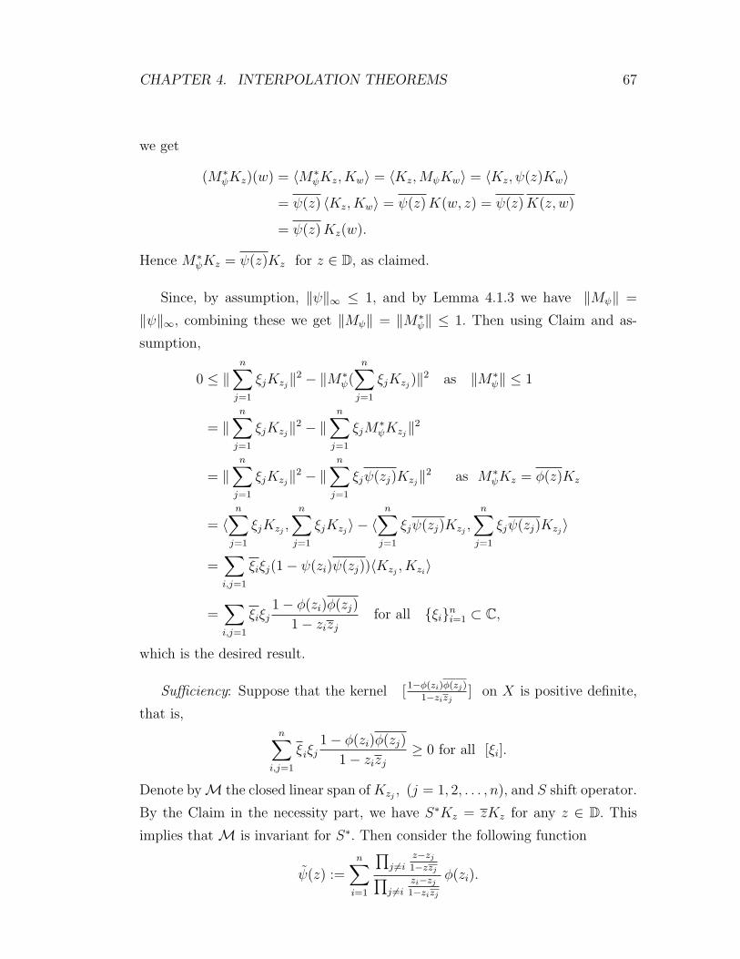
CHAPTER 4. INTERPOLATION THEOREMS 67
we get
(M∗ψKz)(w) = 〈M∗
ψKz, Kw〉 = 〈Kz,MψKw〉 = 〈Kz, ψ(z)Kw〉= ψ(z) 〈Kz, Kw〉 = ψ(z) K(w, z) = ψ(z) K(z, w)
= ψ(z) Kz(w).
Hence M∗ψKz = ψ(z)Kz for z ∈ D, as claimed.
Since, by assumption, ‖ψ‖∞ ≤ 1, and by Lemma 4.1.3 we have ‖Mψ‖ =
‖ψ‖∞, combining these we get ‖Mψ‖ = ‖M∗ψ‖ ≤ 1. Then using Claim and as-
sumption,
0 ≤ ‖n∑
j=1
ξjKzj‖2 − ‖M∗
ψ(n∑
j=1
ξjKzj)‖2 as ‖M∗
ψ‖ ≤ 1
= ‖n∑
j=1
ξjKzj‖2 − ‖
n∑j=1
ξjM∗ψKzj
‖2
= ‖n∑
j=1
ξjKzj‖2 − ‖
n∑j=1
ξjψ(zj)Kzj‖2 as M∗
ψKz = φ(z)Kz
= 〈n∑
j=1
ξjKzj,
n∑j=1
ξjKzj〉 − 〈
n∑j=1
ξjψ(zj)Kzj,
n∑j=1
ξjψ(zj)Kzj〉
=∑i,j=1
ξiξj(1− ψ(zi)ψ(zj))〈Kzj, Kzi
〉
=∑i,j=1
ξiξj1− φ(zi)φ(zj)
1− zizj
for all ξini=1 ⊂ C,
which is the desired result.
Sufficiency: Suppose that the kernel [1−φ(zi)φ(zj)
1−zizj] on X is positive definite,
that is,n∑
i,j=1
ξiξj1− φ(zi)φ(zj)
1− zizj
≥ 0 for all [ξi].
Denote byM the closed linear span of Kzj, (j = 1, 2, . . . , n), and S shift operator.
By the Claim in the necessity part, we have S∗Kz = zKz for any z ∈ D. This
implies that M is invariant for S∗. Then consider the following function
ψ(z) :=n∑
i=1
∏j 6=i
z−zj
1−zzj∏j 6=i
zi−zj
1−zizj
φ(zi).
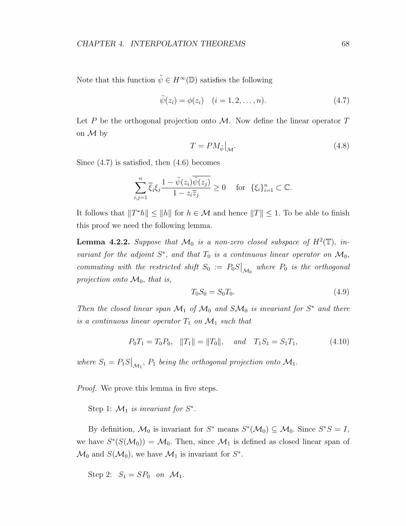
CHAPTER 4. INTERPOLATION THEOREMS 68
Note that this function ψ ∈ H∞(D) satisfies the following
ψ(zi) = φ(zi) (i = 1, 2, . . . , n). (4.7)
Let P be the orthogonal projection onto M. Now define the linear operator T
on M by
T = PMψ
∣∣M. (4.8)
Since (4.7) is satisfied, then (4.6) becomes
n∑i,j=1
ξiξj1− ψ(zi)ψ(zj)
1− zizj
≥ 0 for ξini=1 ⊂ C.
It follows that ‖T ∗h‖ ≤ ‖h‖ for h ∈ M and hence ‖T‖ ≤ 1. To be able to finish
this proof we need the following lemma.
Lemma 4.2.2. Suppose that M0 is a non-zero closed subspace of H2(T), in-
variant for the adjoint S∗, and that T0 is a continuous linear operator on M0,
commuting with the restricted shift S0 := P0S∣∣M0
where P0 is the orthogonal
projection onto M0, that is,
T0S0 = S0T0. (4.9)
Then the closed linear span M1 of M0 and SM0 is invariant for S∗ and there
is a continuous linear operator T1 on M1 such that
P0T1 = T0P0, ‖T1‖ = ‖T0‖, and T1S1 = S1T1, (4.10)
where S1 = P1S∣∣M1
, P1 being the orthogonal projection onto M1.
Proof. We prove this lemma in five steps.
Step 1: M1 is invariant for S∗.
By definition, M0 is invariant for S∗ means S∗(M0) ⊆ M0. Since S∗S = I,
we have S∗(S(M0)) = M0. Then, since M1 is defined as closed linear span of
M0 and S(M0), we have M1 is invariant for S∗.
Step 2: S1 = SP0 on M1.
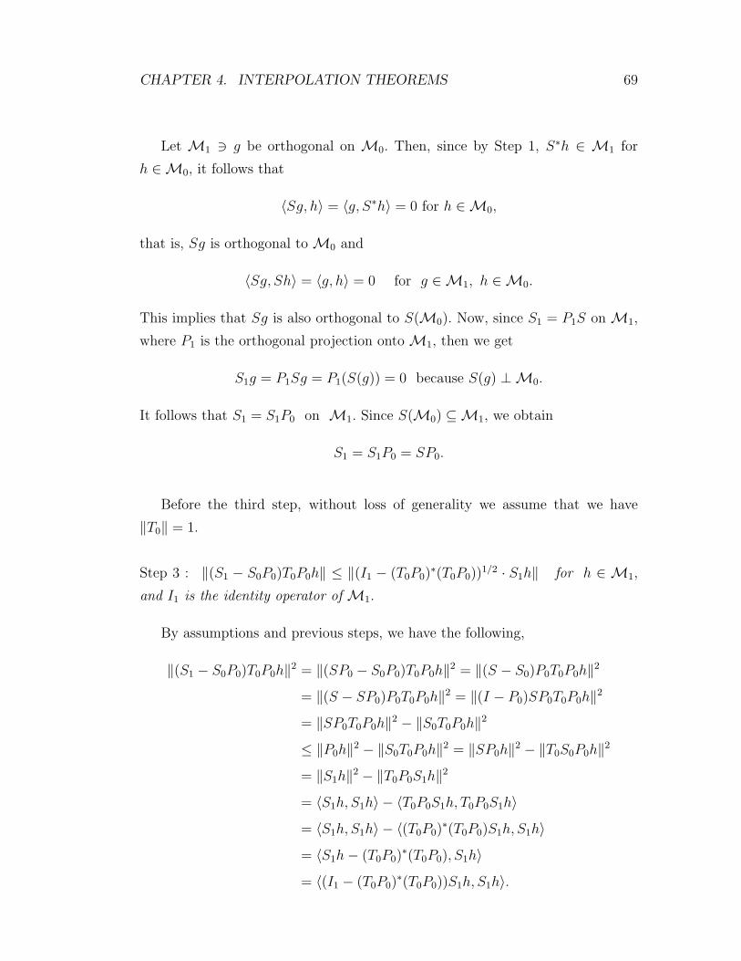
CHAPTER 4. INTERPOLATION THEOREMS 69
Let M1 3 g be orthogonal on M0. Then, since by Step 1, S∗h ∈ M1 for
h ∈M0, it follows that
〈Sg, h〉 = 〈g, S∗h〉 = 0 for h ∈M0,
that is, Sg is orthogonal to M0 and
〈Sg, Sh〉 = 〈g, h〉 = 0 for g ∈M1, h ∈M0.
This implies that Sg is also orthogonal to S(M0). Now, since S1 = P1S on M1,
where P1 is the orthogonal projection onto M1, then we get
S1g = P1Sg = P1(S(g)) = 0 because S(g) ⊥M0.
It follows that S1 = S1P0 on M1. Since S(M0) ⊆M1, we obtain
S1 = S1P0 = SP0.
Before the third step, without loss of generality we assume that we have
‖T0‖ = 1.
Step 3 : ‖(S1 − S0P0)T0P0h‖ ≤ ‖(I1 − (T0P0)∗(T0P0))
1/2 · S1h‖ for h ∈ M1,
and I1 is the identity operator of M1.
By assumptions and previous steps, we have the following,
‖(S1 − S0P0)T0P0h‖2 = ‖(SP0 − S0P0)T0P0h‖2 = ‖(S − S0)P0T0P0h‖2
= ‖(S − SP0)P0T0P0h‖2 = ‖(I − P0)SP0T0P0h‖2
= ‖SP0T0P0h‖2 − ‖S0T0P0h‖2
≤ ‖P0h‖2 − ‖S0T0P0h‖2 = ‖SP0h‖2 − ‖T0S0P0h‖2
= ‖S1h‖2 − ‖T0P0S1h‖2
= 〈S1h, S1h〉 − 〈T0P0S1h, T0P0S1h〉= 〈S1h, S1h〉 − 〈(T0P0)
∗(T0P0)S1h, S1h〉= 〈S1h− (T0P0)
∗(T0P0), S1h〉= 〈(I1 − (T0P0)
∗(T0P0))S1h, S1h〉.
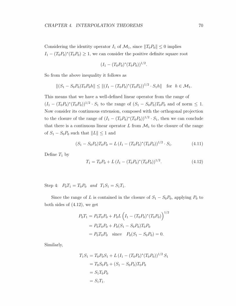
CHAPTER 4. INTERPOLATION THEOREMS 70
Considering the identity operator I1 of M1, since ‖T0P0‖ ≤ 0 implies
I1 − (T0P0)∗(T0P0) ≥ 1, we can consider the positive definite square root
(I1 − (T0P0)∗(T0P0))
1/2.
So from the above inequality it follows as
‖(S1 − S0P0)T0P0h‖ ≤ ‖(I1 − (T0P0)∗(T0P0))
1/2 · S1h‖ for h ∈M1.
This means that we have a well-defined linear operator from the range of
(I1 − (T0P0)∗(T0P0))
1/2 · S1 to the range of (S1 − S0P0)T0P0 and of norm ≤ 1.
Now consider its continuous extension, composed with the orthogonal projection
to the closure of the range of (I1 − (T0P0)∗(T0P0))
1/2 · S1, then we can conclude
that there is a continuous linear operator L from M1 to the closure of the range
of S1 − S0P0 such that ‖L‖ ≤ 1 and
(S1 − S0P0)T0P0 = L (I1 − (T0P0)∗(T0P0))
1/2 · S1. (4.11)
Define T1 by
T1 = T0P0 + L (I1 − (T0P0)∗(T0P0))
1/2. (4.12)
Step 4: P0T1 = T0P0 and T1S1 = S1T1.
Since the range of L is contained in the closure of S1 − S0P0, applying P0 to
both sides of (4.12), we get
P0T1 = P0T0P0 + P0L(I1 − (T0P0)
∗(T0P0))1/2
= P0T0P0 + P0(S1 − S0P0)T0P0
= P0T0P0 since P0(S1 − S0P0) = 0.
Similarly,
T1S1 = T0P0S1 + L (I1 − (T0P0)∗(T0P0))
1/2 S1
= T0S0P0 + (S1 − S0P0)T0P0
= S1T0P0
= S1T1.
CHAPTER 4. INTERPOLATION THEOREMS 71
Hence
P0T1 = T0P0 and T1S1 = S1T1.
Step 5: ‖T1‖ = ‖T0‖.
Since P0L = 0, we have
‖T1h‖2 = ‖T0P0h‖2 + ‖L (I1 − (T0P0)∗(T0P0))
1/2h‖2
≤ ‖T0P0h‖2 + ‖h‖2 − ‖T0P0h‖2 by ‖L‖ ≤ 1
= ‖h‖2,
which yields ‖T1‖ ≤ 1 = ‖T0‖.
Conversely,
‖T0‖ = ‖T0P0‖ = ‖P0T1‖ ≤ ‖T1‖.So we have ‖T1‖ = ‖T0‖.
Therefore T1 satisfies all the requirements in (4.10) of Lemma.
Let us return to the proof of sufficiency part of previous theorem. To avoid
confusion, let us take M0 := M and T0 := T in Lemma. We have that M0 is
invariant under S∗ and ‖T0‖ ≤ 1. Since T0 = P0Mψ
∣∣M0
and S0 = P0S∣∣M0
and
M0⊥ is invariant under S and Mψ, we have P0MψP0 = P0Mψ and P0SP0 = P0S
such that
T0S0 = P0MψP0S∣∣M0
= P0MψS∣∣M0
= P0SMψ
∣∣M0
= S0T0.
Now we can change our theorem into the lemma in such a way that, we have to
find a sequence of linear operators Tn on Mn, the closed linear span of Mn−1
and S(Mn−1), (n = 1, 2, . . .), such that
Pn−1Tn = Tn−1Pn−1, ‖Tn‖ = ‖Tn−1‖ and TnSn = SnTn, (4.13)
where, for each n, Pn is the orthogonal projection onto Mn and Sn = PnS∣∣Mn
.
By Corollary 4.1.6, the closed linear span of Mn : n = 0, 1, . . . which is equal
to that of Sn(M0) : n = 0, 1, . . . must coincide with H2(T). This means that,
Pn strongly converges to I as n →∞. By the equation (4.13) , we reach
‖TnPn‖ ≤ 1 and PnTmPm = TnPn for n ≤ m, (4.14)
CHAPTER 4. INTERPOLATION THEOREMS 72
and hence it follows that there is a continuous linear operator T∞ on H2(T) such
that
‖T∞‖ ≤ 1 and PnT∞ = TnPn for n = 0, 1, . . . (4.15)
Claim: T∞S = ST∞.
Since Pn strongly converges to I as n →∞, then SnPn strongly converges to
S. By (4.15), we have T∞ = limn→∞ PnTnPn. These imply
ST∞ = S limn→∞
PnTnPn = limn→∞
SnTnPn
= limn→∞
TnSnPn by (4.13)
= T∞( limn→∞
SnPn) = T∞S.
Then by Theorem 4.1.5, there exists ψ ∈ H∞(D) such that
‖ψ‖∞ ≤ 1 and Mψ = T∞. (4.16)
Then by (4.15) and (4.16) we reach to
P0Mψ
∣∣M0
= P0T∞∣∣M0
= T0.
Finally, by (4.7) and (4.16),
φ(zi)
1− |zi|2 = φ(zi)〈Kzi, Kzi
〉 = 〈T0Kzi, Kzi
〉
= 〈T∞Kzi, Kzi
〉 = 〈MψKzi, Kzi
〉
=ψ(zi)
1− |zi|2 .
Hence ψ satisfies all the requirements in (4.5) of Theorem 4.2.1.
In the following corollary we consider interpolation on an infinite subset of
the unit disc.
Corollary 4.2.3. Let X be an infinite subset of D, and φ a function on X. In
order for there to exist a function ψ ∈ H∞(D) such that
‖ψ‖∞ ≤ 1 and ψ(z) = φ(z) for z ∈ X, (4.17)
it is necessary and sufficient that the kernel [1−φ(zi)φ(zj)
1−zizj] on X is positive definite.
CHAPTER 4. INTERPOLATION THEOREMS 73
Proof. This follows by an application of Zorn’s Lemma and the previous theorem.
4.3 Interpolation on the Boundary
We will end this chapter by a theorem of interpolation on the boundary of unit
disk D. Before this we need the following lemma.
Lemma 4.3.1. Let Λ be a measurable subset of T and φ a bounded measurable
function on Λ. Then in order for there to exist ψ ∈ H∞(D) such that
‖ψ‖∞ ≤ 1 and ψ(ζ) = φ(ζ) for ζ ∈ Λ σ − a.e., (4.18)
it is necessary and sufficient that
‖P+(φχΛ f)‖ ≤ ‖P+(χΛ f)‖ for f ∈ L2(T). (4.19)
Proof. Suppose that (4.18) is satisfied for ψ ∈ H∞(D). Then
‖P+(φχΛ f)‖ = supg∈H2(D), ‖g‖≤1
|〈φχΛ f, g〉| = supg∈H2(D), ‖g‖≤1
|〈χΛ f, ψ g〉|
≤ ‖ψ‖∞‖P+(χΛ f)‖≤ ‖P+(χΛ f)‖ since ‖ψ‖∞ ≤ 1.
Hence (4.19) is satisfied.
Conversely, suppose that (4.19) is satisfied. Since by Corollary 4.1.8
P+(χΛ f) : f ∈ L2(T) is a dense subspace of H2(T), then there exists an
operator T such that
‖T‖ ≤ 1 and TP+(χΛ f) = P+(φχΛ f) for f ∈ L2(T).
Claim: TS∗ = S∗T.
CHAPTER 4. INTERPOLATION THEOREMS 74
Denote by S the multiplication by the function k(ζ) := ζ in L2(T). Then we
have S∗P+ = P+S∗. It follows that
S∗TP+(χΛ f) = S∗P+(φχΛ f) = P+S∗(φχΛ f)
= P+(φχΛ S∗f) = TP+(χΛ S∗f)
= TP+(S∗(χΛ f)) = TS∗P+(χΛ f).
Since P+(χΛ f) : f ∈ L2(T) is dense in H2(T), the above equation implies
S∗T = TS∗.
By Theorem 4.1.5 there exists ψ ∈ H∞(D) such that
‖ψ‖∞ = ‖T ∗‖ ≤ 1 and T ∗ = Mψ.
Finally, it remains to show ψ(ζ) = φ(ζ) for ζ ∈ Λ σ− a.e. Take f ∈ L2(T). Then
∫
Λ
ψ(ζ)f(ζ)dσ(ζ) = 〈T ∗l, χΛ f〉 = 〈T ∗l, P+(χΛ f)〉
= 〈l, TP+(χΛ f)〉 = 〈l, P+(φχΛ f)〉
= 〈l, φ χΛ f〉 =
∫
Λ
φ(ζ) ˜f(ζ)dσ(η)
which yields that
ψ(ζ) = φ(ζ) for ζ ∈ Λ, σ − a.e.
Theorem 4.3.2. Let Λ be a measurable subset of T with positive σ-measure and φ
a bounded measurable function on Λ. Then in order for there to exist ψ ∈ H∞(D)
such that
‖ψ‖∞ ≤ 1 and ψ(ζ) = φ(ζ) for ζ ∈ Λ σ − a.e., (4.20)
it is necessary and sufficient that
limr→1
∫
Λ
∫
Λ
(1− φ(ξ)φ(ζ)
1− r2ξζ
)f(ξ)f(ζ)dσ(ξ)dσ(ζ) ≥ 0 for all f ∈ L2(T). (4.21)
Proof. Recall that in Chapter 2, the orthogonal projection PH2 was expressed in
terms of the Szego kernel;
(PH2g)(z) = 〈g, Kz〉L2 , for z ∈ D and g ∈ L2(T),
CHAPTER 4. INTERPOLATION THEOREMS 75
and
(PH2g)(ζ) = limr→1〈g, Krζ〉 for almost all ζ ∈ T.
Then for 0 < r < 1 and η ∈ T, by above equations we get the followings;
(P+g)(rη) =
∫
Tg(ζ)
1
1− rηζdσ(ζ)
and
limr→1
∫
T|(P+g)(rη)− (P+g)(η)|2dσ(η)
= limr→1
∫
T
∣∣∫
Tg(ζ)(
1
1− rηζ)dσ(ζ)−
∫
Tg(ζ)(
1
1− ηζ)dσ(ζ)
∣∣2dσ(η)
= limr→1
∫
T
∣∣∫
Tg(ζ)(
1
1− rηζ− 1
1− ηζ)dσ(ζ)
∣∣2dσ(η)
= limr→1
∫
T
∣∣∫
Tg(ζ)(
rηζ − ηζ
1− ηζ − rηζ + rη|ζ|2 )dσ(ζ)∣∣2dσ(η)
= 0.
It follows that
‖P+g‖2 = 〈P+g, P+g〉 = limr→1
∫
T|(P+g)(rη)|2dσ(η)
= limr→1
∫
T
( ∫
T
∫
T
g(ζ)
1− rηζ
g(ε)
1− rηεdσ(ε)dσ(ζ)
)dσ(η)
= limr→1
∫
T
∫
T
( ∫
T
1
1− rηζ
1
1− rηεdσ(η)
)g(ε)g(ζ)dσ(ε)dσ(η)
= limr→1
∫
T
∫
T〈Krη, Krε〉 g(ε)g(ζ)dσ(ε)dσ(η)
= limr→1
∫
T
∫
T
1
1− r2εζg(ε)g(ζ)dσ(ε)dσ(η).
Therefore for all g ∈ L2(T), we have
‖P+g‖2 = limr→1
∫
T
∫
T
1
1− r2εζg(ε)g(ζ)dσ(ε)dσ(η). (4.22)
Since by previous lemma we have (4.19) by (4.18), these imply
‖P+(χΛ g)‖2 − ‖P+(φχΛ g)‖2 ≥ 0.
Then it follows by (4.22) that
limr→1
∫
Λ
∫
Λ
(1− φ(ξ)φ(ζ)
1− r2ξζ
)g(ξ)g(ζ)dσ(ξ)dσ(ζ) ≥ 0 for all g ∈ L2(T).
Appendix A
Hilbert Spaces
A.1 Definitions
Definition A.1.1. Let H be a linear space over the complex field C. An inner
product on H is a function 〈·, ·〉 : H × H → C which satisfies the following
conditions:
(i) 〈f, g〉 = 〈g, f〉 for f, g ∈ H.
(ii) 〈λf + µg, h〉 = λ〈f, h〉+ µ〈g, h〉 and
〈f, λg + µh〉 = λ〈f, g〉+ µ〈f, h〉 for λ, µ ∈ C and f, g and h ∈ H.
(iii) 〈f, f〉 ≥ 0 for f ∈ H and 〈f, f〉 = 0 if and only if f = 0.
Definition A.1.2. A pre-Hilbert space (inner product space) H is a linear space
over C with an inner product defined on it.
If H is an inner product space, ‖ · ‖ defines a norm on H by
‖f‖ = 〈f, f〉1/2.
Sometimes we use the notations ‖ · ‖H and 〈·, ·〉H for norm and inner product,
respectively.
76
APPENDIX A. HILBERT SPACES 77
Some important properties:
‖f‖ ≥ 0 and equality occurs only when f = 0. (A.1)
‖ξf‖ = |ξ|‖f‖ for f ∈ H, ξ ∈ C. (A.2)
|〈f, g〉| ≤ ‖f‖‖g‖ for f, g ∈ H (Schwarz Inequality), (A.3)
and equality occurs when f and g are linearly dependent.
‖f + g‖ ≤ ‖f‖+ ‖g‖ for f, g ∈ H (Triangular Inequality), (A.4)
and equality occurs when f and g are linearly dependent.
〈f, g〉 =1
4(‖f + g‖2 − ‖f − g‖2 + i‖f + ig‖2 − ‖f − ig‖2) for f, g ∈ H (A.5)
(polarization identity).
‖f+g‖2+‖f−g‖2 = 2‖f‖2+2‖g‖2 for f, g ∈ H (parallelogram identity). (A.6)
Define d(f, g) := ‖f − g‖ the binary function. Observe that for f, g and h ∈ Hand for all ξ ∈ C, d satisfies all requirements to be a metric:
(i) d(f, g) ≥ 0 and equality occurs if and only if f = g.
(ii) d(f, g) = d(g, f).
(iii) d(f, g) ≤ d(f, h) + d(h, g).
(iv) d(f − h, g − h) = d(f, g) (translation invariant).
(v) d(ξf, ξg) = |ξ| · d(f, g).
This binary function introduces metric topology in H which is called strong
topology or norm topology.
In other words a sequence (f)n≥0 in H converges strongly to f if ‖fn−f‖ →0 as n →∞.
APPENDIX A. HILBERT SPACES 78
Definition A.1.3. A map L from a linear space to another is called linear oper-
ator if it satisfies
L(ηf + ζg) = ηLf + ζLg
for η, ζ ∈ C and f, g ∈ H.
The operator L is continuous if L is continuous at each point of domain of
L. To be able to speak of continuity of a linear operator, the domain and range
spaces have to be equipped with respective topologies.
Let L be a linear operator from H to G with H and G are pre-Hilbert spaces.
The Lipschitz constant for a linear operator L is called its norm and denoted by
‖L‖ where
‖L‖ = sup‖Lf‖G/‖f‖H : 0 6= f ∈ H. (A.7)
Theorem A.1.4. Let L be a linear operator from H to G where H and G are
pre-Hilbert spaces. The followings are mutually equivalent:
(i) L is continuous
(ii) L is bounded in the sense that
sup‖Lf‖G : ‖f‖H ≤ σ < ∞
for 0 ≤ σ < ∞.
(iii) L is Lipschitz continuous in the sense that there is 0 ≤ γ < ∞ such
that
‖Lf − Lg‖G ≤ γ‖f − g‖H,
for f, g ∈ H.
Proof. (i)=⇒(ii)
Let L be continuous. Define a neighborhood of 0 in G as v = g : ‖g‖G 5 1.Continuity of L implies L0 = 0 and there is a neighborhood (of 0 in H) of the
form u = f : ‖f‖H 5 δ which is mapped into v by L, where δ > 0. Now let
APPENDIX A. HILBERT SPACES 79
us take a nonzero f ∈ H such that ‖f‖H 5 ρ, for ρ > 0. Since ‖δf/ρ‖H ≤ δ,
then δfρ∈ u. As L is linear,
δ‖Lf‖G/ρ = ‖L(δf/ρ)‖G 5 1
and
sup‖Lf‖G : ‖f‖H 5 ρ 5 ρ
δ.
(ii)=⇒ (iii)
Let L satisfies (ii). Consider the norm of Lf − Lg. By linearity property of
L,
‖Lf − Lg‖G = ‖L(f − g)‖G 5 γ‖f − g‖H for f, g ∈ H,
where γ is the supremum in (ii) with ρ = 1.
(iii)=⇒ (i)
This is obvious since boundedness implies continuity.
Denote by B(H,G), all continuous linear operators from H to G, H and G are
pre-Hilbert spaces. B(H,G) becomes a linear space with respect to the natural
addition and scalar multiplication:
(ξL + ζM)f = ξLf + ζMf,
where L and M are linear operators, f ∈ H and ξ ∈ C.
When H = G, B(H,G) is denoted by B(H).
Let K be another pre-Hilbert space. If L ∈ B(H,G) and K ∈ B(G,K), then
their product will be KL ∈ B(H,K) and defined by
(KL)f = K(Lf) for f ∈ H.
Moreover we have the following properties:
(i) K(ξL + ζM) = ξKL + ζKM
APPENDIX A. HILBERT SPACES 80
(ii) ‖ξL‖ = |ξ| · ‖L‖
(iii) ‖L + M‖ ≤ ‖L‖+ ‖M‖ and
(iv) ‖KL‖ ≤ ‖K‖‖L‖.
For H,G are pre-Hilbert spaces and L,M are linear operators, B(H,G) be-
comes a metric space with respect to the translation invariant, positively homoge-
nous distance function
d(L,M) := ‖L−M‖.
For each K ∈ B(G,K), the map L 7−→ KL becomes a continuous linear
operator from B(H,G) to B(H,K).
Definition A.1.5. A linear operator from H to the scalar field C is called a
linear functional (or linear form).
Definition A.1.6. A pre-Hilbert spaceH is called a Hilbert space if it is complete
in metric. In other words, if fn is a Cauchy sequence in H, i.e. ‖fn − fm‖ −→ 0
when n,m →∞, then there is f ∈ H such that ‖fn − f‖ −→ 0 when n →∞.
Every subspace of a pre-Hilbert space is again a pre-Hilbert space with respect
to the induced inner product; but for a subspace of a Hilbert space to be again a
Hilbert space, it has to be closed.
Let H be a pre-Hilbert space. We can imbed H as a dense subspace of a
Hilbert space H in such a way that
〈f, g〉H = 〈f, g〉H for f, g ∈ H.
This canonical method is called completion. If we have a continuous linear opera-
tor L from a dense subspace M of a Hilbert space H to a Hilbert space G, we can
extend L uniquely to a continuous linear operator from H to G with preserving
norm.
Theorem A.1.7. Let M be a dense subspace of a Hilbert space H, and N a
dense subspace of a Hilbert space G. If a linear operator L from M to G satisfies
APPENDIX A. HILBERT SPACES 81
|〈Lf, g〉G| ≤ |γ|‖f‖H‖g‖G for f ∈ H, g ∈M with some 0 ≤ γ < ∞, (A.8)
then it is uniquely extended to a continuous linear operator from M to G with
norm ≤ γ. The minimum of such γ coincides with norm.
Proof. Let L be a linear operator from M to G and satisfies (A.8). By fixing f ,
since g 7−→ 〈Lf, g〉G and g 7−→ ‖g‖G are continuous, we can assume that (A.8)
is satisfied for all g ∈ G.
Now by using (A.8) and Schwarz inequality, we get
‖Lf‖G2 = 〈Lf, Lf〉G ≤ γ‖f‖H‖Lf‖G
which implies
‖Lf‖G ≤ γ‖f‖H for all f ∈ M.
Hence L is continuous operator from M to G with norm ≤ γ. So we can
extend L uniquely to a continuous linear operator from H to G with preserving
norm. It is obvious that minimum of γ coincides with norm.
Theorem A.1.8. Let L2(Ω, µ) consists of all measurable functions f(ω) on Ω
such that ∫
Ω
|f(ω)|2dµ(ω) < ∞, (A.9)
where (Ω, µ) is a measure space such that Ω is the union of subsets of finite
positive measure. Then L2(Ω, µ) becomes a Hilbert space with respect to the inner
product
〈f, g〉 :=
∫
Ω
f(ω)g(ω)dµ(ω). (A.10)
Proof. We have
|f(ω) + g(ω)|2 ≤ 2|f(ω)|2 + |g(ω)|2which implies that L2(Ω, µ) is a linear space. If we expand the left handside, we
have
|f(ω) + g(ω)|2 = |f(ω)|2 + |g(ω)|2 + 2f(ω)g(ω) ≤ 2|f(ω)|2 + |g(ω)|2
APPENDIX A. HILBERT SPACES 82
which implies that
|f(ω)g(ω)| ≤ 1
2|f(ω)|2 + |g(ω)|2.
So, 〈f, g〉 in (A.10) is well-defined and the linear space L2(Ω, µ) becomes a
pre-Hilbert space.
Completeness :
Let us take a Cauchy sequence (fn)n≥1 in L2(Ω, µ). Suppose that
∞∑n=1
‖fn+1 − fn‖ ≡ γ < ∞.
For any m, consider the following integration,∫
Ω
m∑n=1
|fn+1(ω)− fn(ω)|2dµ(ω) ≤∞∑
n=1
‖fn+1 − fn‖2 = γ2 < ∞.
Then by the Lebesque theorem,∫
Ω
∞∑n=1
|fn+1(ω)− fn(ω)|2dµ(ω) ≤ γ2 < ∞
which implies
g(ω) ≡m∑
n=1
|fn+1(ω)− fn(ω)| < ∞ for almost all ω,
and∫
Ω
g(ω)2dµ(ω) =
∫
Ω
∞∑n=1
|fn+1(ω)− fn(ω)|2dµ(ω) ≤ γ2 < ∞.
Hence for almost all ω , the sequence (fn(ω))n≥1 converges. To find the limit of
f(ω), consider the following
|fn+1(ω)− fn(ω)|2 ≤∞∑
k=n
|fk+1(ω)− fk(ω)|2
≤m∑
n=1
|fn+1(ω)− fn(ω)| = g(ω)
and again by Lebesque theorem,
limn→∞
‖fn − f‖2 = limn→∞
〈fn − f, fn − f〉 = limn→∞
∫
Ω
|fn(ω)− f(ω)|2dµ(ω)
≤∫
Ω
limn→∞
|fn(ω)− f(ω)|2dµ(ω) = 0.
APPENDIX A. HILBERT SPACES 83
Therefore fn converges strongly to f , which means L2(Ω, µ) is complete and
it is a Hilbert space with respect to the given inner product.
Let H and G be Hilbert spaces. The algebraic direct sum of H and G, con-
sisting of f⊕g with the functions f ∈ H and g ∈ G, becomes a Hilbert space,
denoted by H⊕G with respect to the inner product
〈f⊕g, f ′⊕g′〉 = 〈f, f ′〉H + 〈g, g′〉G.
Let H and G be Hilbert spaces. The algebraic tensor product of H and G,
consisting of finite sums of f⊗g with f ∈ H and g ∈ G, becomes a pre-Hilbert
space with respect to the inner product
〈∑
i
fi⊗gi,∑
j
f ′j⊗g′j〉 =∑i,j
〈fi, f′j〉H · 〈gi, g
′j〉G.
Definition A.1.9. The canonical completion of the algebraic tensor product of
H and G, where H and G are Hilbert spaces, is called tensor product Hilbert space
and denoted by H⊗G.
A.2 Projection
We start this section with an important theorem.
Theorem A.2.1 (F.Riesz). For each continuous linear functional φ on a Hilbert
space H, there exists uniquely g ∈ H such that
φ(f) = 〈f, g〉 for f ∈ H. (A.11)
Proof. For the case φ = 0, take g = 1, then we are done.
Let φ 6= 0. For this case, we can suppose that ‖φ‖ = 1. Then there exists a
sequence gn such that
‖gn‖ = 1 (n = 1, 2, ..) and φ(gn) −→ ‖φ‖ = 1 as n →∞.
APPENDIX A. HILBERT SPACES 84
Then by parallelogram rule
‖gm − gn‖2 + ‖gm + gn‖2 = 2‖gm‖2 + 2‖gn‖2 = 2 + 2 = 4.
On the other hand by triangular rule,
2 = ‖gm‖+ ‖gn‖ ≥ ‖gm + gn‖,
then we get
2 ≥ ‖gm + gn‖ ≥ |φ(gm) + φ(gn)| −→ 2 as m,n →∞.
Thus,
‖gm + gn‖ = 2 and ‖gm + gn‖2 = 4. So, ‖gm − gn‖ −→ 0 as m,n →∞.
Then, due to the metric completeness, gn converges strongly to some g such
that ‖g‖ = φ(g) = 1.
Let f ∈ H be arbitrary. If 〈f, g〉 = 0, then for all ζ ∈ C,
‖g + ζf‖2 = ‖g‖2 + ζ〈g, f〉+ ζ〈f, g〉+ |ζ|2‖f‖2 = 1 + |ζ|2‖f‖2
and
‖g + ζf‖2 ≥ |φ(g + ζf)|2 = |φ(g) + ζφ(f)|2 = |1 + ζφ(f)|2
= 1 + 2Reζφ(f) + |ζ|2|φ(f)|2.
Combining these equations, we get
1 + |ζ|2‖f‖2 ≥ 1 + 2Reζφ(f) + |ζ|2|φ(f)|2.
Since ζ is arbitrary, then φ(f) = 0. This implies
φ(f) = 〈f, g〉 for f satisfying 〈f, g〉 = 0.
Now consider the other case which is 〈f, g〉 6= 0. Define h := f − 〈f, g〉g. It
follows that,
〈h, g〉 = 〈f − 〈f, g〉g, g〉 = 〈f, g〉 − 〈〈f, g〉g, g〉 = 〈f, g〉 − 〈f, g〉 = 0.
APPENDIX A. HILBERT SPACES 85
Then,
0 = φ(h) = φ(f)− 〈f, g〉φ(g) = φ(f)− 〈f, g〉.Hence we obtain φ(f) = 〈f, g〉.
To see the uniqueness of g, suppose that there exists g′ ∈ H such that for
each linear functional φ, we have
φ(f) = 〈f, g′〉.
Also this equality is satisfied for g. Thus we have
φ(f) = 〈f, g′〉 = 〈f, g〉
which implies
〈f, g − g′〉 = 0.
Hence g = g′.
Theorem A.2.2. For any closed subspace M of a Hilbert space H,
H = M⊕M⊥ (algebraic direct sum),
that is, each f ∈ H can be uniquely written in the form
f = fM + fM⊥ with fM ∈M, fM⊥ ∈M⊥. (A.12)
Moreover, ‖fM‖ coincides with the distance from f to M⊥;
‖fM‖ = min‖f − g‖ : g ∈M⊥, (A.13)
the distance being attained only at fM⊥ .
Proof. Since M is closed, it is also a Hilbert space. By Riesz theorem to the
continuous functional h 7−→ 〈h, g〉 restricted to M, there is fM ∈ M, such
that
〈h, f〉 = 〈h, fM〉 for h ∈M.
By this, we get 〈h, f − fM〉 = 0. Let us define fM⊥ := f − fM. Since
〈h, f − fM〉 = 0, then fM⊥ ⊥ h for all h ∈M. So, fM⊥ ∈M⊥. Hence
f = fM + fM⊥ where fM ∈M, fM⊥ ∈M⊥.
APPENDIX A. HILBERT SPACES 86
For the uniqueness, let f = f ′M + f ′M⊥ be any other decomposition of f , where
f ′M ∈M, f ′M⊥ ∈M⊥. Then,
f = f ′M + f ′M⊥ = fM + fM⊥
which implies that
fM − f ′M = fM⊥ − f ′M⊥
and by the last equality we obtain that fM = f ′M.
For the moreover part, let us take any g ∈ M⊥. Since 〈fM⊥ − g, f〉 = 0, we
get
‖f − g‖2 = ‖fM + fM⊥ − g‖2 = ‖fM‖2 + ‖fM⊥ − g‖2.
Then we have
‖f − g‖2 ≥ ‖fM‖2 and equality occurs when g = fM⊥ .
Hence,
‖fM‖ = min‖f − g‖ : g ∈M⊥.
Corollary A.2.3. In a Hilbert space, the closed linear span of any subset A
coincides with (A⊥)⊥.
Proof. Let M be the closed linear span of A. So, we have M ⊆ (A⊥)⊥. It
remains to show the other side of inclusion. As (A⊥)⊥ is a closed subspace
of H, so it is also a Hilbert space. Now by using the Theorem A.2.2, for each
f ∈ (A⊥)⊥, f has a decomposition such that f = g + h where g ∈ M, h ∈(A⊥)⊥ and h is orthogonal to all of M. Since A ⊆M, h must be orthogonal
to all of A. In other words, h must be in A⊥. But h is both in A⊥ and (A⊥)⊥. Hence
h = 0 and h = 0 = f − g implies f = g ∈ M i.e. (A⊥)⊥ ⊆ M. Consequently,
M = (A⊥)⊥.
Definition A.2.4. A subset of a Hilbert space H is said to be total (complete)
in H if 0 is the only element that is orthogonal to all of A, i.e. A⊥ = 0.
APPENDIX A. HILBERT SPACES 87
So by the Corollary A.2.3, A is total if and only if every element of H can be
approximated by linear combinations of elements of A.
Definition A.2.5. When M is a closed subspace of H, the map f 7−→ fM
determines a linear operator from H to M with norm ≤ 1. This operator is
called the orthogonal projection to M and is denoted by PM.
If I is the identity operator, then I − PM becomes the orthogonal projection
to M⊥ and
‖f‖2 = ‖PMf‖2 + ‖(I − PM)f‖2. (A.14)
Theorem A.2.6 (Abstract Interpolation). Let H be a Hilbert space, X an
index set and γ a positive number. Given a map x 7−→ fx from X to H and one
x 7−→ ax from X to C, there exists an element g ∈ H such that
‖g‖ ≤ γ and 〈fx, g〉 = ax for x ∈ X, (A.15)
if and only if
∑x,y
ξyξxayax ≤ γ2∑x,y
ξyξx〈fx, fy〉 for [ξx], (A.16)
where [ξx] denotes, in general, a function on X which vanishes outside a finite
number of points.
Proof. Suppose that (A.15) is satisfied for g ∈ H. Then
∑x,y
ξyξxayax = |∑
x
ξxax|2 = |∑
x
ξx〈fx, g〉|2 = |〈∑
x
ξxfx, g〉|2,
by the Schwarz inequality
≤ ‖∑
x
ξxfx‖2‖g‖2 ≤ γ2‖∑
x
ξxfx‖2 = γ2∑x,y
ξyξx〈fx, fy〉.
So (A.16) is satisfied.
Now suppose (A.16) is satisfied. Then the correspondence
∑x
ξxfx 7−→∑
x
ξxax
APPENDIX A. HILBERT SPACES 88
defines a linear functional on the linear span of fx : x ∈ X with norm ≤ γ.
This bounded functional can be extended to the closure of this linear span, and
then by using Riesz’s Representation Theorem (see Theorem A.2.1) the vector g
can be found such that ‖g‖ ≤ γ and 〈fx, g〉 = ax for all x ∈ X.
A.3 Weak Topology
Definition A.3.1. The weak topology of a Hilbert space H is the weakest topol-
ogy that makes continuous all linear functionals of the form f 7−→ 〈f, g〉.
For an element f in the weak topology, a fundamental system of neighborhoods
of f consists of subsets of the form
U(f ; A, ε) = h : |〈f, g〉 − 〈h, g〉| < ε for g ∈ A,
where A is a finite subset of H and ε is a positive number. Then a directed net
fλ converges weakly to f if and only if
〈fλ, g〉 λ−→ 〈f, g〉
for all g ∈ H.
Definition A.3.2. The (operator) weak topology in the space B(H,G) of contin-
uous linear operators from H to a Hilbert space G, is the weakest topology that
makes continuous all linear functionals of the form L 7−→ 〈Lf, g〉 for f ∈ H and
g ∈ G.
Then a directed net Lλ converges (operator) weakly to L if and only if
〈Lλf, g〉 λ−→ 〈Lf, g〉.
Definition A.3.3. The (operator) strong topology is the weakest topology that
makes continuous all linear operators of the form L 7−→ Lf for f ∈ H.
APPENDIX A. HILBERT SPACES 89
Then a directed net Lλ converges (operator) strongly to L if and only if
‖Lλf − Lf‖ λ−→ 0
for all f ∈ H.
Theorem A.3.4 ([1]). The closed unit ball U := f : ‖f‖ ≤ 1 of a Hilbert
space H is weakly compact.
Theorem A.3.5 ([1]). The closed unit ball L : ‖L‖ ≤ 1 of B(H,G) is
(operator) weakly compact.
Theorem A.3.6. If a subset A of a Hilbert space H is weakly bounded in the
sense
supf∈A
|〈f, g〉| < ∞ for g ∈ H, (A.17)
then it is strongly bounded, that is, supf∈A ‖f‖ < ∞.
Proof. Define
Bn := g : |〈f, g〉| ≤ n for f ∈ A, (n = 1, 2, 3, . . .).
Then for each n, Bn will be a closed subset of H and so H =⋃
n Bn. By Baire
category theorem, since H is a complete metric space with respect to the strong
topology and H is covered by a countable number of closed sets, then at least
one of them has nonempty interior, say Bn0 . So, for some g0 and ε > 0,
V ≡ g : ‖g − g0‖ ≤ ε ⊂ Bn0
Let g be in H. Since
‖g0 + εg/‖g‖ − g0‖ = ‖|ε|g/‖g‖‖ ≤ ε,
then g0 + εg/‖g‖ will be in V . Then
ε|〈f, g〉|/‖g‖ ≤ |〈f, g0 + εg/‖g‖〉|+ |〈f, g0〉| ≤ n0 + n0 = 2n0 for f ∈ A.
This implies,
|〈f, g〉| ≤ 2n0‖g‖/ε for f ∈ A.
APPENDIX A. HILBERT SPACES 90
Putting f instead of g in the last inequality and using Schwarz inequality, we
get
supf∈A
≤ 2n0/ε < ∞.
Theorem A.3.7. Let H and G be Hilbert spaces. For a linear operator L from
H to G , strong continuity and weak continuity are the same thing.
Proof. Let L be weakly continuous. Since by Theorem A.3.4 the unit ball U of a
Hilbert space is weakly compact, it follows that L(U) is also weakly compact and
so weakly bounded in G. Since Theorem A.3.6 states that weakly boundedness
implies strongly boundedness, L(U) will be strongly bounded and hence it is
strongly continuous by TheoremA.1.4
Now suppose that L is strongly continuous. So we have, for each g ∈ G, the
linear functional f 7−→ 〈Lf, g〉G is continuous on H. Now by Riesz theorem, there
is g′ ∈ H such that,
f 7−→ 〈f, g′〉H for f ∈ H,
then
〈Lf, g〉G = 〈f, g′〉H for f ∈ H.
Hence L is weakly continuous.
Theorem A.3.8 ([1]). Let H and G be Hilbert spaces. Then the following as-
sertions for a subset L of B(H,G) are mutually equivalent:
(i) L is (operator) weakly bounded;
supL∈ L
|〈Lf, g〉| < ∞ for f ∈ H, g ∈ G.
(ii)L is (operator) strongly bounded;
supL∈ L
‖Lf‖ < ∞ for f ∈ H.
(iii) L is norm bounded (or uniformly bounded);
supL∈ L
‖L‖ < ∞.
APPENDIX A. HILBERT SPACES 91
Definition A.3.9. A linear operator L from H to G, where H and G are Hilbert
spaces, is said to be closed if its graph
GL := f⊕Lf : f ∈ H (A.18)
is a closed subspace of the direct sum space H⊕G, that is, if |fn− f‖ −→ 0 in Has (n →∞) and ‖Lfn − g‖ −→ 0 in G as (n →∞), then g = Lf.
Theorem A.3.10. Any closed linear operator L from a Hilbert space H to an-
other Hilbert space G is continuous.
Proof. Let GL be the graph of L. Since L is closed, then GL is a closed subspace
and so it is a Hilbert space. Consider the linear operator φ : f⊕Lf 7−→ f from
GL to H. φ is a bijection because of closedness of GL. Let UL be the unit ball
of GL. By Theorem A.3.4 UL is weakly compact. This implies φ(UL) is weakly
compact and so is⋃∞
n=1 nφ(UL) = H. Now by Baire theorem, φ(UL) has non-
empty interior. By the proof of Theorem A.3.6, there exists 0 ≤ γ < ∞ such
that
‖f⊕Lf‖ ≤ γ‖f‖ for f ∈ H.
This implies
‖f⊕Lf‖2 = 〈‖f⊕Lf‖, ‖f⊕Lf‖〉 = 〈f, f〉+ 〈Lf, Lf〉 = ‖f‖2 + ‖Lf‖2 ≤ γ2‖f‖2.
Then we obtain
‖Lf‖ ≤ (γ2 − 1)1/2‖f‖.Hence L is continuous.
Corollary A.3.11 ([1]). Every continuous linear bijection between Hilbert spaces
has continuous inverse.
A.4 Self-adjoint Operators
Definition A.4.1. Let H and G are Hilbert spaces. A function Φ : H×G −→ Cis a sesquilinear form (or function) if for f, h ∈ H, g, k ∈ G and α, β ∈ C,
(i) Φ(αf + βh, g) = αΦ(f, g) + βΦ(h, g) (A.19)
APPENDIX A. HILBERT SPACES 92
(ii) Φ(f, αg + βk) = αΦ(f, g) + βΦ(f, k) (A.20)
are satisfied.
If L ∈ B(H,G), then the sesquilinear form Φ is defined as
Φ(f, g) = 〈Lf, g〉G (A.21)
and it is bounded,
|Φ(f, g)| ≤ γ‖f‖H‖g‖G for f ∈ H, g ∈ G, (A.22)
where γ can take any value not less than ‖L‖.
If we are given a sesqui-linear form Φ satisfies boundedness condition (A.22),
then for fixed f ∈ H, the linear functional g 7−→ Φ(f, g) is continuous on G.
Applying Riesz theorem, there exists uniquely f ′ ∈ G such that
‖f ′‖G ≤ γ‖f‖H and Φ(f, g) = 〈f ′, g〉G for g ∈ G.
Then f 7−→ f ′ becomes linear, so we obtain Φ(f, g) = 〈f ′, g〉G = 〈Lf, g〉G.
Definition A.4.2. If L ∈ B(H,G), then there exists a unique operator in
B(G,H), called adjoint of L, denoted by L∗ satisfying
Φ(f, g) = 〈f, L∗g〉H for f ∈ H, g ∈ G. (A.23)
By the definition of L and L∗, we have the following relation,
〈Lf, g〉G = 〈f, L∗g〉H for f ∈ H, g ∈ G. (A.24)
Some other properties of adjoint operator:
‖L‖ = ‖L∗‖. (A.25)
Given H,G and K are Hilbert spaces, if K ∈ B(G,K) and L ∈ B(H,G),
then
KL ∈ B(H,K) and (KL)∗ = L∗K∗. (A.26)
APPENDIX A. HILBERT SPACES 93
ker L = (RanL∗)⊥ and (ker L)⊥ = closureRanL∗ (A.27)
where ker L is the kernel of L and RanL is the range of L.
Theorem A.4.3 ([1]). For L,M ∈ B(H,G), the following assertions are mutu-
ally equivalent.
(i) Ran(M) ⊆ Ran(L).
(ii) There exists K ∈ B(H) such that M = LK.
(iii) There exists 0 ≤ γ < ∞ such that
‖M∗g‖ ≤ γ‖L∗g‖ for g ∈ G.
Definition A.4.4. Let H be a Hilbert space. A function φ : H −→ C is a
quadratic form if for all f ∈ H and ζ ∈ C,
φ(ζf) = |ζ|2φ(f) (A.28)
and
φ(f + g) + φ(f − g) = 2φ(f) + φ(g) (A.29)
are satisfied.
For L ∈ B(H), the quadratic form φ on H is defined as
φ(f) = 〈Lf, f〉 for f ∈ H, (A.30)
and it is bounded
|φ(f)| ≤ γ‖f‖2 for f ∈ H, (A.31)
where γ can take any value not less than ‖L‖.
The sesqui-linear form Φ associated with L can be recaptured from quadratic
form φ by the following equation:
Φ(f, g) =1
4φ(f + g)− φ(f − g)+ φ(f + ig)− φ(f − ig) (A.32)
for all f, g ∈ H.
APPENDIX A. HILBERT SPACES 94
Definition A.4.5. A continuous linear operator L on a Hilbert space H is said
to be self-adjoint if L = L∗.
Remark A.4.6. L is self adjoint if and only if the associated sesqui-linear form
Φ is Hermitian.
Remark A.4.7. If L is self-adjoint, norm of L coincides with the minimum of
γ in (A.31) for the associated quadratic form.
Theorem A.4.8. If L is a continuous self-adjoint operator, then
‖L‖ = sup|〈Lf, f〉| : ‖f‖ ≤ 1. (A.33)
Proof. Let γ = sup|〈Lf, f〉| : ‖f‖ ≤ 1.It is obvious that γ ≤ ‖L‖. Consider the reverse direction. By the Remark A.4.6,
since L is self-adjoint, then associated quadratic form is Hermitian, so real-valued.
Let fix f, g ∈ H and choose eiθ such that
〈L(eiθf), g〉 = |〈Lf, g〉|.
Then using the equality (A.32), it follows that
|〈Lf, g〉| = Re〈L(eiθf), g〉
=1
4〈L(eiθf + g), eiθf + g〉 − 〈L(eiθf − g), eiθf − g〉
≤ γ
4‖eiθf + g‖2 + ‖eiθf − g‖2 =
γ
2‖f‖2 + ‖g‖2.
Now replace f and g by λf andg
λrespectively, and take the minimum in λ, we
obtain
|〈Lf, g〉| ≤ γ‖f‖‖g‖ for f, g ∈ H.
Hence we have
‖L‖ ≤ γ.
Definition A.4.9. A self-adjoint operator L ∈ B(H) is said to be positive definite
if 〈Lf, f〉 ≥ 0 for all f ∈ H. If 〈Lf, f〉 = 0 only when f = 0, then L is said to
be strictly positive definite.
APPENDIX A. HILBERT SPACES 95
Remark A.4.10. For any positive definite operator L ∈ B(H), a generalized
Schwarz inequality holds:
|〈Lf, g〉|2 ≤ 〈Lf, f〉 · 〈Lg, g〉. (A.34)
Theorem A.4.11. Let L and M be continuous positive definite operators on Hand G respectively. A continuous linear operator K from H to G satisfies the
inequality
|〈Kf, g〉G|2 ≤ 〈Lf, f〉H〈Mg, g〉G for f ∈ H, g ∈ G (A.35)
if and only if the continuous linear operator
[L K∗
K M
]
on the direct sum Hilbert space H⊕G:
f⊕g 7−→ (Lf + K∗g)⊕(Kf + Mg)
is positive definite.
Proof. Suppose that (A.35) is satisfied. Let S stands for the matrix
[L K∗
K M
]
such that
〈S(f⊕g), f⊕g〉 = 〈Lf + K∗g, f〉H + 〈Kf + Mg, g〉G,then by using the property of adjoint operator and Schwarz inequality, the above
equation follows as
〈S(f⊕g), f⊕g〉 = 〈Lf, f〉H + 〈K∗g, f〉H + 〈Kf, g〉G + 〈Mg, g〉G= 〈Lf, f〉H + 〈g,Kf〉G + 〈Kf, g〉G + Mg, g〉G= 〈Lf, f〉H + 2Re〈Kf, g〉G + 〈Mg, g〉G≥ 〈Lf, f〉H + 〈Mg, g〉G − 2
√〈Lf, f〉H〈Mg, g〉G
= √〈Lf, f〉H −
√〈Mg, g〉G2 ≥ 0.
APPENDIX A. HILBERT SPACES 96
Thus S is positive definite.
Conversely, let S be positive definite. By the above relation we have
0 ≤ 〈S(f⊕g), f⊕g〉 = 〈Lf + K∗g, f〉H + 〈Kf + Mg, g〉G= 〈Lf, f〉H + 〈K∗g, f〉H + 〈Kf, g〉G + 〈Mg, g〉G
then replacing g with a suitable eiθg, we get
〈Lf, f〉H − 2|〈Kf, g〉G|+ 〈Mg, g〉G ≥ 0,
or
|〈Kf, g〉G| ≤ 1
2〈Lf, f〉H + 〈Mg, g〉G .
Then replacing f and g by λf andg
λrespectively, we obtain
|〈Kf, g〉G|2 ≤ 〈Lf, f〉H〈Mg, g〉G.
Theorem A.4.12 ([1]). Let L be a continuous positive definite operator. Then
there exists uniquely a positive definite operator called the square root of L, de-
noted by L1/2, such that (L1/2)2 = L.
Definition A.4.13. For a continuous linear operator L, the square root of the
positive definite operator L∗L is called the modulus (operator) of L.
Definition A.4.14. A linear operator V between Hilbert spaces H and G is
called isometric or an isometry if it preserves the norm, that is,
‖V f‖G = ‖f‖H for f ∈ H. (A.36)
By (A.36), a continuous linear operator V is isometric if and only if V ∗V = IH,
in other words, V preserves inner product :
〈V f, V g〉G = 〈f, g〉H for f, g ∈ H. (A.37)
Definition A.4.15. A linear operator U : H −→ H that is a surjective isometry
is called a unitary (operator).
APPENDIX A. HILBERT SPACES 97
If U ∈ B(H) is a unitary operator, then U∗ = U−1.
Definition A.4.16. A continuous linear operator U between Hilbert spaces Hand G is called a partial isometry if for f ∈ (ker U)⊥ = Ran(U∗), ‖Uf‖ = ‖f‖.The space (ker U)⊥ is called the initial space of U and the space Ran(U) is called
the final space of U.
For a partial isometry U , its adjoint U∗ is again a partial isometry.
Corollary A.4.17 ([1]). Each continuous linear operator L on H admits a
unique decomposition
L = UL, (A.38)
where L is positive definite and U is a partial isometry with initial space the
closure of Ran(L). Indeed, L must be the modulus |L|.
Bibliography
[1] T. Ando, Reproducing Kernel Spaces and Quadratic Inequalities, Lecture
Notes, Hokkaido University, Research Institute of Applied Electricity, Divi-
sion of Applied Mathematics, Sapporo, Japan, 1987.
[2] N. Aronszajn, Theory of reproducing kernels, Trans. Amer. Math. Soc.
68(1950), 337–404.
[3] J.B. Conway, A Course in Functional Analysis, Springer Verlag, Berlin -
Heidelberg - New York, 1989.
[4] P.L. Duren, Theory of Hp Spaces, Academic Press, INC., New York, 1970.
[5] P.L. Duren, A. Schuster, Bergman Spaces, Amer. Math. Soc., Provi-
dence R.I. 2004.
[6] H. Dym, J-Contractive Matrix Functions, Reproducing Kernel Hilbert
Spaces and Interpolation, CBMS Regional Conference Series in Mathematics,
Amer. Math. Soc., Providence R.I. 1989.
[7] P. Koosis, Introduction to Hp Spaces, Cambridge Mathematical Press,
Cambridge, 1970.
[8] S. Saitoh, Theory of Reproducing Kernels and its Applications, Pitman
Research Notes in Mathematics Series, vol. 189, Longman Scientific and
Technical, Harlow, 1988.
[9] J. Weidman, Linear Operators in Hilbert Spaces, Springer Verlag, Berlin -
Heidelberg - New York, 1980.
98