DOCUMENT RESUME

ED 463 346 UD 034 861

AUTHOR Lochner, Lance; Moretti, EnricoTITLE The Effect of Education on Crime: Evidence from Prison

Inmates, Arrests, and Self-Reports.PUB DATE 2001-12-00NOTE 52p.

PUB TYPE Numerical/Quantitative Data (110) -- Reports - Research(143)

EDRS PRICE MF01/PC03 Plus Postage.DESCRIPTORS Black Students; Compulsory Education; *Crime; Crime

Prevention; *Delinquency; *Educational Attainment;Graduation; High Schools; Racial Differences; *Role ofEducation

IDENTIFIERS *Incarcerated Youth

ABSTRACTThis paper estimates the effect of education on

participation in crime and incarceration, using data from the U.S. Census andchanges in state compulsory attendance laws. Increases in compulsoryschooling ages are not correlated with increases in state resources devotedto fighting crime. Research suggests that additional years of secondaryschooling reduce the probability of incarceration, with the greatest impactassociated with completing high school. Black-white differences ineducational attainment explain up to 23 percent of the gap in incarcerationrates. FBI arrest data corroborate findings on incarceration. The mainimpacts of education relate to murder, assault, and motor vehicle theft. Thestudy examines the effect of schooling on self-reported crime in the NationalLongitudinal Survey of Youth, noting that estimates for imprisonment andarrest are caused by changes in criminal behavior, not educationaldifferences in the probability of arrest or incarceration conditional oncrime. The study calculates social savings from crime reduction associatedwith high school graduation. The externality is about 14-26 percent of theprivate return, suggesting that a significant part of the social return tocompleting high school comes in the form of externalities from crimereduction. (Contains 12 tables and 37 references.) (SM)

Reproductions supplied by EDRS are the best that can be madefrom the ori inal document.

The Effect of Education on Crime: Evidence fromPrison Inmates, Arrests, and Self-Reports

Lance LochnerEnrico Moretti

PERMISSION TO REPRODUCE ANDDISSEMINATE THIS MATERIAL HAS

BEEN GRANTED BY

LI Lac.i.i.oc'fic

TO THE EDUCATIONAL RESOURCESINFORMATION CENTER (ERIC)

1

(X)

BEST COPY AVAILABLE2

U.S. DEPARTMENT OF EDUCATIONOffice of Educational Research and Improvement

EDUCATIONAL RESOURCES INFORMATIONCENTER (ERIC)

0 This document has been reproduced asreceived from the person or organizationoriginating it.

0 Minor changes have been made toimprove reproduction quality.

Points of view or opinions stated in thisdocument do not necessarily representofficial OERI position or policy.

The Effect of Education on Crime: Evidence from Prison Inmates,

Arrests, and Self-Reports*

Lance Lochner Enrico MorettiDepartment of Economics Department of EconomicsUniversity of Rochester UCLA

December 2001

Abstract

This paper estimates the effect of education on participation in criminal activity accounting

for endogeneity of schooling. Crime is a negative externality with enormous social costs, so if

education reduces crime, then schooling may have large social benefits that are not taken into

account by individuals.The paper begins by analyzing the effect of schooling on incarceration using Census data

and changes in state compulsory attendance laws over time as an instrument for schooling.

Changes in these laws have a significant effect on educational achievement, and we reject tests

for reverse causality. Moreover, increases in compulsory schooling ages are not correlated with

increases in state resources devoted to fighting crime. Both OLS and IV estimates agree and

suggest that additional years of secondary schooling reduce the probability of incarceration

with the greatest impact associated with completing high school. Differences in educational

attainment between blacks and whites can explain as much as 23% of the black-white gap in

incarceration rates.We corroborate our findings on incarceration using FBI data on arrests that distinguish

among different types of crimes. The biggest impacts of education are associated with murder,

assault, and motor vehicle theft. We also examine the effect of schooling on self-reported crime

in the NLSY and find that our estimates for imprisonment and arrest are caused by changes in

criminal behavior and not educational differences in the probability of arrest or incarceration

conditional on crime. Given the consistency of our estimates, we calculate the social savings

from crime reduction associated with high school graduation. The externality is about 14-26%

of the private return, suggesting that a significant past of the social return to completing high

school comes in the form of externalities from crime reduction.

*We are grateful to Daron Acemoglu and Josh Angrist for their data on compulsory attendance laws and useful

suggestions. We thank Mark Bib, Elizabeth Caucutt, Janet Currie, Gordon Dahl, Stan Engerman, Jeff Grogger,

David Levine, Jens Ludwig, Darren Lubotsky, Marco Manacorda, David Mustard, Steve Rivkin, Edward Vytlacil

and seminar participants at Columbia University, Chicago GSB, NBER Summer Institute, Econometric Society,

University of Rochester, UCLA, University of British Columbia, Hoover Institution, and Stanford University for

their helpful comments.

1

3

1 Introduction

Is it possible to reduce crime rates by raising the education of potential criminals? If so, would it

be cost effective with respect to other crime prevention measures? Despite the enormous policy

implications, little is known about the relationship between schooling and criminal behavior.

The motivation for these questions is not limited to the obvious policy implications for crime

prevention. Estimating the effect of education on criminal activity may shed some light on the

magnitude of the social return to education. Economists interested in the benefits of schooling

have traditionally focused on the private return to education. However, researchers have recently

started to investigate whether schooling generates benefits beyond the private returns received

by individuals. In particular, a number of studies attempt to determine whether the schooling

of one worker raises the earnings of other workers around him. (For example, see Acemoglu and

Angrist (2000), Heckman and Klenow, (1999), and Moretti (1999).) Yet, little research has been

undertaken to evaluate the importance of other types of external benefits of education, such as

its potential effects on crime. (Lochner (1999) and Witte (1997) are notable exceptions.) Crime

is a negative externality with enormous social costs. If education reduces crime, then schooling

will have social benefits that are not taken into account by individuals. In this case, the social

return to education may exceed the private return. Given the large social costs of crime, even

small reductions in crime associated with education may be economically important.

There are a number of reasons to believe that education can reduce criminal activity. First,

schooling increases the returns to legitimate work, raising the opportunity costs of illegal behav-

ior.1 Additionally, punishment for criminal behavior often entails incarceration. By raising wage

rates, schooling makes any time spent out of the labor market more costly. Second, schooling

may directly affect the financial or psychic rewards from crime itself. Finally, schooling may

alter preferences in indirect ways, which may affect decisions to engage in crime. For example,

education may increase one's patience (as in Becker and Mulligan (1997)) or risk aversion.

Despite the many reasons to expect a causal link between education and crime, empirical

research is not conclusive.2 The key difficulty in estimating the effect of education on criminal

'Freeman (1996), Gould, et al. (2000), Grogger (1998), Machin and Meghir (2000), and Viscusi (1986) empiri-cally establish a negative correlation between earnings levels (or wage rates) and criminal activity. The relationshipbetween crime and unemployment has been more tenuous (see Chiricos (1987) or Freeman (1983, 1995) for excel-lent surveys); however, a number of recent studies that better address problems with endogeneity and unobservedcorrelates (including Gould, et al. (2000) and Raphael and Winter-Ebmer (2001)) find a sizeable positive effect ofunemployment on crime.

2Witte (1997) concludes that "...neither years of schooling completed nor receipt of a high school degree has asignificant affect on an individual's level of criminal activity." But, this conclusion is based on only a few availablestudies, including Tauchen, et al. (1994) and Witte and Tauchen (1994), which find no significant link betweeneducation and crime after controlling for a number of individual characteristics. While Grogger (1998) estimates asignificant negative relationship between wage rates and crime, he finds no relationship between education and crimeafter controlling for wages. (Of course, increased wages are an important consequence of schooling.) More recently,Lochner (1999) estimates a significant and important link between high school graduation and crime using data

14

activity is that unobserved characteristics affecting schooling decisions are likely to be correlated

with unobservables influencing the decision to engage in crime. For example, individuals with high

criminal returns or discount rates are likely to spend much of their time engaged in crime rather

than work regardless of their educational background. To the extent that schooling does not

raise criminal returns, there is little reward to finishing high school or attending college for these

individuals. As a result, we might expect a negative correlation between crime and education

even if there is no causal effect of education on crime. State policies may induce bias with the

opposite sign if increases in state spending for crime prevention and prison construction trade

off with spending for public education, a positive spurious correlation between education and

crime is also possible.

In this paper, we use individual-level data on incarceration from the Census and cohort-level

data on arrests by state from the FBI Uniform Crime Reports (UCR) to analyze the effects of

schooling on crime. We then turn to self-report data on criminal activity from the National

Longitudinal Survey of Youth (NLSY) to verify that the estimated impacts measure changes in

crime and not educational differences in the probability of arrest or incarceration conditional

on crime. We employ a number of empirical strategies to account for unobservable individual

characteristics and state policies that may introduce spurious correlation.

We start by analyzing the effect of education on incarceration. The group quarters type

of residence in the Census indicates whether an individual is incarcerated at the Census date.

For both blacks and whites, OLS estimates uncover significant reductions in the probability of

incarceration associated with more schooling. To address endogeneity problems, we use changes

in state compulsory attendance laws over time to instrument for schooling. Changes in these laws

have a significant effect on educational achievement, and we reject tests for reverse causality. In

the years preceding increases in compulsory schooling laws, there is no obvious trend in schooling

achievement. Increases in education associated with increased compulsory schooling take place

after changes in the law. Furthermore, increases in the number of years of compulsory attendance

raise high school graduation rates but have no effect on college graduation rates. These two facts

indicate that the increases in compulsory schooling raise education, not vice versa. We also

examine whether increases in compulsory schooling ages are associated with increases in state

resources devoted to fighting crime. They are not.

Instrumental variable estimates reveal a significant relationship between education and incar-

ceration, and they suggest that the impacts are greater for blacks than for whites. One extra

from the National Longitudinal Survey of Youth (NLSY). Other research relevant to the link between educationand crime has examined the correlation between crime and time spent in school (Gottfredson 1985, Farrington

et al. 1986, Witte and Tauchen 1994). These studies find that time spent in school significantly reduces criminalactivity more so than time spent at work suggesting a contemporaneous link between school attendance andcrime. Previous empirical studies have not controlled for the endogeneity of schooling.

5

year of schooling results in a .10 percentage point reduction in the probability of incarceration

for whites, and a .37 percentage point reduction for blacks. To help in interpreting the size of

these impacts, we calculate how much of the black-white gap in incarceration rates in 1980 is due

to differences in educational attainment. Differences in average education between blacks and

whites can explain as much as 23% of the black-white gap in incarceration rates.

Because incarceration data do not distinguish between types of offenses, we also examine the

impact of education on arrests using data from the UCR. This data allows us to identify the

type of crime that arrested individuals have been charged with. Estimates uncover a robust and

significant effect of high school graduation on arrests for both violent and property crimes, effects

which are consistent with the magnitude of impacts observed for incarceration in the Census data.

When arrests are separately analyzed by crime, the greatest impacts of graduation are associated

with murder, assault, and motor vehicle theft.

Estimates using arrest and imprisonment measures of crime may confound the effect of edu-

cation on criminal activity with educational differences in the probability of arrest and sentencing

conditional on commission of a crime. To verify that our estimates identify a relationship be-

tween education and actual crime, we estimate the effects of schooling on self-reported criminal

participation using data from the NLSY. These estimates confirm that education significantly

reduces self-reported participation in both violent and property crime. We also use the NLSY

to explore the robustness of our findings on imprisonment to the inclusion of rich measures of

family background and individual ability. The OLS estimates obtained in the NLSY controlling

for AFQT scores, parental education, family income, and several other background characteristics

are remarkably similar to the estimates obtained using Census data.

Given the general consistency in findings across data sets, measures of criminal activity, and

identification strategies, we cannot reject that a relationship between education and crime exists.

Using our estimates, we calculate the social savings from crime reduction associated with high

school completion. Our estimates suggest that a 1% increase in malehigh school graduation rates

would save as much as $1.4 billion, or about $2,100 per additional male high school graduate.

These social savings represent an important externality of education that has not yet been doc-

umented. The estimated externality from education ranges from 14-26% of the private return to

high school graduation, suggesting that a significant part of the social return to education is in

the form of externalities from crime reduction.

The remainder of the paper is organized as follows. In Section 2, a simple model of criminal

activity is described. Section 3 reports estimates of the impact of schooling on incarceration

rates (Census data), and Section 4 reports estimates of the impact of schooling on arrest rates

(UCR data). Section 5 uses NLSY data on self-reported crime and on incarceration to check the

robustness of UCR and Census-based estimates. In Section 6, we calculate the social savings from

crime reduction associated with high school graduation. Section 7 concludes.

2 An Economic Framework

To provide some intuition as to why education might affect criminal behavior, this section dis-

cusses a simple economic model of work, school, and crime. The model is by no means a complete

description of criminal decisionmaking, but it is a useful reference point for an empirical study of

crime and schooling. Individuals are assumed to choose the amount of education they acquire and

the amount of time spent on work and crime once they have finished school. We begin by ana-

lyzing crime and work decisions conditional on educational choice, then return to the educational

choice problem.

Consider the decisions of someone who has completed s years of school and must decide how

to allocate his time to work and crime, where kt is the fraction of time spent committing crime at

age t. Let Wt(s) represent his wage rate and R(kt, s) his total net return from crime at age t if he

has s years of schooling.3 Assume that someone who commits crime in period t has a probability,

71-(kt), of being punished the next period, t + 1, where 711(kt) > 0. For simplicity, assume that

the punishment, P, is constant over time and measured in utility terms. While in school, an

individual receives a constant utility of U. Since we are interested in post-school crime, we ignore

crime during school years. At each age after completing school, individuals consume their income

from work and crime, receiving utility u(yt), where yt = wt(s)(1 kt) R(kt, s) is total income

in period t, u'(yt) > 0 and u"(yt) < 0. The individual's maximization problem, conditional on

already having chosen s years of school, is

lt 1V (s) = ma. Efiu+os- E p t (s)[u(wt(s)(1 kt) + R(kt, s)) P(s)7r(kt)P]{k}- 8+1

It=o t=s+1

where 0 E [0, I] is an individual's initial discount factor, p(s) E [0, 1] is his after-school discount

factor (i.e. schooling may affect his rate of time preference), and T is the total number of years

he can work or attend school. V (s) represents the lifetime value of choosing s years of school

when the individual chooses his criminal behavior optimally.

The interior first order condition for crime, kt, is given by

OR(kt, s) Cr' (kt)PWt(s) = P(s) 0. (1)

akt

Notice, the gap between current returns from crime and work must be (weakly) positive, since

crime involves future punishment. The right hand side of equation (1) represents the compen-

sating differential that must be paid in the criminal sector due to potential punishment. It is

'In the analysis that follows, we assume that w(s) > 0, w(s) > a, and Pe > 0.

4

7

increasing in the discount rate p(s), since impatient individuals (low p(s)) heavily discount future

punishment costs.

Equation (1) suggests three ways that schooling can affect criminal decisions. First, school-

ing increases individual wage rates, thereby increasing the opportunity costs of crime. Second,

schooling may affect the net marginal returns to crime, gt . Finally, schooling may alter individ-

ual rates of time preference. That is, schooling may increase the patience exhibited by individuals

(i.e. p' (s) > 0).4 As long as schooling increases the marginal return to work more than crime

(1dt (s) > a"kt) and schooling does not decrease patience levels, crime is decreasing in the number

of years of schooling. It is also clear that, all else equal, individuals with higher wage rates and

lower discount factors (p) will commit less crime. High wage rates reduce crime by increasing its

opportunity cost, while increased patience makes delayed punishments more costly.

Recall that schooling is not exogenous. After calculating their optimal lifetime work and crime

decisions for each potential level of schooling, young individuals will choose the education level

that maximizes lifetime earnings, V (s). The same factors that affect decisions to commit crime,

and therefore V (s), also affect schooling decisions. For example, it is clear from equation (1) that

individuals with lower discount factors will engage in more crime, since more impatient individuals

put less weight on future punishments. At the same time, individuals with low discount factors

choose to invest less in schooling, since they discount the future benefits of schooling more heavily.

Similarly, individuals with a high marginal return from crime are likely to spend much of their

time committing crime regardless of their educational attainment. If schooling provides little or

no return in the criminal sector (i.e. 12,181s 0), then there is little value to attending school.

Both examples suggest that schooling and crime are likely to be negatively correlated, even if

schooling has no causal effect on crime.

An Empirical Specification

We now clarify the empirical issues involved in estimation. To simplify the discussion further,

consider an income maximizing framework (u(y) = y) where the probability of facing punishment

is simply 7rkt and the net return to crime depends on individual characteristics 0 according to5

R(kt, s) = (0 + 7(s))kt

4While this specification does not explicitly allow schooling to affect individual tastes for crime, the relationshipbetween schooling and net criminal returns yields qualitatively similar implications. One could also allow for incar-ceration (i.e. punishment may include time out of the criminal and labor market), which would make punishmentsmore costly for those with high wage rates or criminal returns. This would provide another channel through whichschooling affects crime. These additional channels have been suppressed to maintain simplicity.

5We assume throughout this analysis that 0 is unobserved. Introducing observed characteristics is straightfor-ward.

5

8

Solving the first order conditions for kt yields the following characterization for criminal activity:6

kt(0, s) = (1111)(wt(s) + -y(s) + 0 p(s)r.13). If time preferences are unaffected by schooling and

the probability of punishment as well as the punishment itself varies across locations, /, then

criminal behavior for person i at age t is described by

wt(si) Oi P71131ko,t

If the difference in returns to schooling for work and crime is linear in schooling, so (tot(s)

-y(s))1ii = ct + Ss, we obtain a simple reduced form specification for criminal behavior for person

i as

ki,t,t = ct ös i + 9

where ri is the parameter of interest, öi = Oi/71 is a measure of unobserved ability, and d1 = p711P1171

is a state-specific dummy representing the deterrent effect of expected punishment. Standard

OLS regressions of criminal activity on schooling and current location will be biased if individual

criminal abilities or returns (Oi) are correlated with schooling. Indeed, theory suggests that Oi

and si are negatively correlated (i.e. those with high criminal returns will acquire less education)

producing a negative bias in the estimated impact of schooling on crime. Failure to account for

differences in expected punishment levels across location may also induce a bias. If states face

budget decisions between funding for schools and funding for police and prisons, we might expect

a negative correlation between expected punishments and schooling levels across states. In this

case, failure to account for state-level variation in expected punishments would lead to positively

biased estimates.

To address the endogeneity of schooling and eliminate the bias induced by correlation between

Oi and si, we use instruments that exogenously affect schooling choices. Using valid instruments

for schooling and controlling for state-level variation should produce unbiased estimates of 6 in

the simple framework above. A final complication arises due to data limitations. The instruments

that we use in this paper are effective when using large data sets on crime like the Census or

UCR. However, neither of these data sets measures crime directly. The Census data provide

information on incarceration while the UCR provide data on arrests. It is, therefore, important

to clarify the relationship between schooling and these alternative measures of crime.

It is reasonable to assume that arrests and incarceration are a function of the amount of

crime committed, kt. Consider first the case where both the probability of arrest conditional

on crime (7ra) and the probability of incarceration conditional on arrest (7ri) are constant and

age invariant. Then an individual with s years of schooling will be arrested with probability

Pr (Arrestt) = 7rakt(s) and incarcerated with probability Pr(Inct) = 7ri7rakt(s).

6For an interior solution where 0 E (a t(s), a t(s) -I- 77) and a t(s) = zut(s) y(s) p(s)R P .

6

9

Consider two schooling levels high school completion (s=1) and drop out (s=0). Then, the

effect of graduation on crime is simply kt(1) kt(0), while its effect on arrests is ra(kt (1) kt (0)).

Its impact on incarceration is 7rira (kt(1)kt (0)). The measured effects of graduation on arrest and

incarceration rates are less than its effect on crime by factors of 7ra and 7rira, respectively. However,

graduation should have similar effects on crime, arrests, and incarceration when measured in

logarithms.

More generally, the probability of arrest conditional on crime, ra(s), and the probability of

incarceration conditional on arrest, 7ri(s), may depend on schooling. This would be the case if, for

example, more educated individuals have access to better legal defense resources or are treated

more leniently by police officers and judges. In this case, the measured effects of graduation on

arrest and incarceration rates (when measured in logarithms) are

ln Pr(Arrestt ls = 1) ln Pr(Arrestt ls = 0) = (ln kt(1) ln kt(0)) + (In ira (1) ln ira (0))

and

lnPr(Inctls = 1)-1n Pr(Inctls = 0) = (ln kt(1)ln kt(0))+(lnira(1)ln ira(0))+(lnri(1)-1n7ri(0)),

respectively. If the probability of arrest conditional on crime and the probability of incarceration

conditional on arrest are larger for less educated individuals, then the measured effect of gradua-

tion on arrest is greater than its effect on crime by In7ra (1) In7r,(0) and its measured effect on

imprisonment is larger still by the additional amount In r(1) ln ri(0). Mustard (2001) provides

evidence from U.S. federal court sentencing that high school graduates are likely to receive a

slightly shorter sentence than otherwise similar graduates, though the difference is quitel small

(about 2-3%).

3 The Impact of Schooling on Incarceration Rates

3.1 Data and OLS Estimates

We begin by analyzing the impact of education on the probability of incarceration for men using

U.S. Census data. The public versions of the 1960, 1970, and 1980 Censuses report the type of

group quarters and, therefore, allow us to identify prison and jail inmates, who respond to the

same Census questionnaire as the general population. We create a dummy variable equal to 1

if the respondent is in a correctional institution.7 We include in our sample males ages 20-60

for whom all the relevant variables are reported. Summary statistics are provided in Table 1.

Roughly 0.5-0.7% of the respondents are in prison during each of the Census years we examine.

Average years of schooling increase steadily from 10.5 in 1960 to 12.5 in 1980.

7Unfortunately, the public version of the 1990 Census does not identify inmates. The years under considerationprecede the massive prison build-up that began around 1980.

10

Table 2 reports incarceration rates by race and educational attainment. The probability of

imprisonment is substantially larger for blacks than for whites and this is the case for all years and

education categories. Incarceration rates for white men with less than twelve years of schooling

are around .8% while they average about 3.6% for blacks over the three decades. Incarceration

rates are monotonically declining with education for all years and for both blacks and whites.

An important feature to notice in Table 2 is that the reduction in the probability of impris-

onment associated with higher schooling is substantially larger for blacks than for whites. For

example, in 1980 the difference between high school drop outs and college graduates is .8% for

whites and 3.5% for blacks. Because high school drop outs are likely to differ in many respects

from individuals with more education, these differences do not necessarily represent the causal

effect of education on the probability of incarceration. However, the patterns indicate that the

effect may differ for blacks and whites. In the empirical analysis below, we allow for differential

effects by race whenever possible.8

To account for other factors in determining incarceration rates, we begin by using OLS to

examine the impacts of education. Figure 1 shows how education affects the probability of

imprisonment at all schooling levels after controlling for age, state of birth, state of residence,

cohort of birth and year effects (i.e. the graphs display the coefficient estimates on the complete

set of schooling dummies). The figure clearly shows a decline in incarceration rates with schooling

beyond 8th grade, with a larger decline at the high school graduation stage than at any other

schooling progression.

We now present results for models that are either linear in years of schooling or that measure

education using a dummy variable for high school graduation. Table 3 reports the estimated

effects of years of schooling on the probability of incarceration using a linear probability model

(columns 1-3). Estimates for whites are presented in the top panel with estimates for blacks in

the bottom. In column 1, covariates include year dummies, age (14 dummies for three-year age

groups, including 20-22, 23-25, 26-28, etc.), state of birth, and state of current residence, which

are all likely to be important determinants of criminal behavior and incarceration.9 To account

for the many changes that affected Southern born blacks after Brown v. Board of Education, we

also include a state of birth specific dummy for black men born in the South who turn age 14 in

1958 or later. These estimates suggest that an additional year of schooling reduces the probability

of incarceration by 0.001 for whites and by 0.0037 for blacks.th The larger effect for blacks is

8The stability in aggregate incarceration rates reported in Table 1 masks the underlying trends within eacheducation group, which show substantial increases over the 1970s. The substantial difference in high school graduateand drop out incarceration rates combined with the more than 25% increase in high school graduation rates over thistime period explains why aggregate incarceration rates remained relatively stable over time while within educationgroup incarceration rates rose.

8A11 specifications exclude Alaska and Hawaii as a place of birth, since our instruments below are unavailablefor those states.

10The standard errors are corrected for state of birth - year of birth clustering, since our instrument below varies

8

1 1

consistent with the larger differences in unconditional means reported in Table 2.

Column 2 accounts for unobserved differences across birth cohorts, allowing for differences

in school quality or youth environments by including dummies for decade of birth (1914-1923,

1924-1933, etc.). Column 3 further controls for for state of residence x year effects. This absorbs

state-specific time-varying shocks or policies that may affect the probability of imprisonment and

graduation. For example, an increase in prison spending in any given state may be offset by a

decrease in education spending that year. (Notice, however, that since prison inmates may have

committed their crime years before they are observed in prison, the state of residence x year effects

are an imperfect control.) Both sets of estimates are insensitive to these additional controls.

The largest impact of education on imprisonment occurs when moving from less than high

school to high school graduation (see Figure 1 or Table 2). Given the importance of high school

completion in determining incarceration rates, we explore a specification in Table 4 that conditions

on high school graduation rather than total years of schooling. We present results for the two

most general specifications, identical to columns 2 and 3 of Table 3, although other specifications

yield similar estimates. In this table, high school graduates include anyone with 12 or more years

of schooling and a high school degree." OLS estimates in columns 1 and 2 indicate that high

school graduation is associated with a decrease in the probability of imprisonment by about 0.76

percentage points for whites and 3.4 percentage points for blacks.12

Two points about robustness are worth making now. First, in Section 5 we use NLSY data

to show that these results are not sensitive to the inclusion of controls for individual ability

and family background characteristics. In particular, models that include AFQT scores, family

income, parents' education, whether or not the individual lived with both of his natural parents

at age 14 and whether his mother was teenager at his birth estimated using NLSY data yield

estimates that are remarkably similar to those based on Census data. Second, probit models yield

similar estimated effects. We further examine the sensitivity of these results and our IV results

below.

To help in interpreting the size of these impacts on incarceration, one can use these estimates to

calculate how much of the black-white gap in incarceration rates is due to differences in educational

attainment. In 1980, the difference in incarceration rates for whites and blacks is about 2.4%.

at the state of birth year of birth level.11We ignore the fact that in some years, high school graduation in South Carolina could be achieved with 11

years of schooling. We also ignore the fact that some inmates graduate in prison, which is uncommon in the yearswe examine. If some inmates graduate from high school while in prison, these estimates will be biased towardfinding no effect of graduation on crime.

12Both coefficients are larger than the unconditional estimates, 0.06 percentage points for whites and 1.7 forblacks, obtained by simply differencing the average imprisonment rates. The difference between conditional andunconditional estimates is explained by the inclusion of age effects in the conditional specification. Drop out ratesincrease with age in our sample due to the secular trend of increasing education throughout the century andimprisonment rates decrease with age since most crimes are committed by younger men.

9

1 2

Using the estimates for blacks, we conclude that 23% of the difference in incarceration rates

between blacks and whites could be eliminated by raising the average education levels of blacks

to the same level as that of whites.

Alternatively, consider that the rise in white and black high school graduation rates between

1970 and 1980 are 13 and 21 percentage points, respectively.13 In this case, the rise in graduation

rates among whites should have caused a decrease of 0.1 percentage points in their incarceration

rates (compared to a base of 0.6% among white drop outs in 1970). The corresponding figure for

blacks is 0.6 percentage points (compared to a base of 2.9% among black drop outs in 1970).

3.2 The Effect of Compulsory Attendance Laws on Schooling Achievement

The OLS estimates just presented are consistent with the hypothesis that education reduces

the probability of imprisonment. If so, the effect appears to be statistically significant for both

whites and blacks, and quantitatively larger for blacks. However, these estimates may reflect

the effects of unobserved individual characteristics that influence the probability of committing

crime and dropping out of school. For example, the theoretical model in Section 2 suggests that

individuals with a high discount rate or taste for crime, presumably from more disadvantaged

backgrounds, are likely to commit more crime and attend less schooling. To the extent that

variation in unobserved discount rates and criminal proclivity across cohorts is important, OLS

estimates could overestimate the effect of schooling on imprisonment.

It is also possible that juveniles who are arrested or confined to youth authorities while in

high school may face limited educational opportunities. Even though we examine men ages 20

and older, some are likely to have been incarcerated for a few years, and others may be repeat

offenders. If their arrests are responsible for their drop out status, this should generate a negative

correlation between education and crime. Fortunately, this does not appear to be an important

empirical problem.14

The ideal instrumental variable induces exogenous variation in schooling but is uncorrelated

with discount rates and other individual characteristics that affect both imprisonment and school-

ing. We use changes over time in the number of years of compulsory education that states mandate

as an instrument for education. Years of compulsory attendance are defined as the maximum

between (i) the minimum number of years that a child is required to stay in school and (ii) the

difference between the earliest age that he is required to be in school and the latest age he is

"These graduation rates refer to the proportion of 20-60 year old men with a high school degree and not the

graduation rate of cohorts from those years."A simple calculation using NLSY data suggests that the bias introduced by this type of reverse causality is

small. The incarceration gap between high school graduates and drop outs among those who were not in jail at ages

17 or 18 is 0.044, while the gap for the full sample is only slightly larger (0.049). Since the first gap is not affected

by reverse causality, at most 10% of the measured gap can be explained away by early incarceration resulting indrop out. If some of those who were incarcerated would have dropped out anyway (not an unlikely scenario), less

than 10% of the gap is eliminated.

required to enroll. Figure 2 plots the evolution of compulsory attendance laws over time for 49

states (all but Alaska and Hawaii). In the years relevant for our sample, 1914 to 1974, states

changed compulsory attendance levels several times, and not always upward.

We assign compulsory attendance laws to individuals on the basis of state of birth and the

year when the individual was 14 years old. To the extent that individuals migrate across states

between birth and age 14, the instrument precision is diminished, though IV estimates will still

be consistent. We create four indicator variables, depending on whether years of compulsory

attendance are 8 or less, 9, 10, and 11 or 12.15 The fractions of individuals belonging to each

compulsory attendance group are reported in Table 1.

Figure 3 shows how the increases in compulsory schooling affect educational attainment over

time, controlling for state and year of birth.16 In the 12 years before the increase, there is no

obvious trend in schooling achievement. All of the increase in schooling associated with stricter

compulsory schooling laws takes place after changes in the law. This figure is important because

it suggests that changes in compulsory schooling laws are not simply picking up underlying trends

in education. Stricter compulsory attendance laws appear to raise education, not vice versa. More

formal tests of reverse causality are provided below.

Table 5 quantifies the effect of compulsory attendance laws on educational achievement. These

specifications include controls for age, year, state of birth, state of residence, and cohort of birth

effects. To account for the impact of Brown v. Board of Education on the schooling achievement

of Southern born blacks, they also include an additional state of birth dummy for black cohorts

born in the South turning age 14 in 1958 or later. Identification of the estimates comes from

changes over time in the number of years of compulsory education in any given state. The

identifying assumption is that conditional on state of birth, cohort of birth, state of residence and

year, the timing of the changes in compulsory attendance laws within each state is orthogonal

to characteristics of individuals that affect criminal behavior like family background, ability, risk

aversion, or discount rates.

Consider the estimates for whites presented in the top panel. Three points are worth making.

First, the more stringent the compulsory attendance legislation, the lower, is the percentage of

high school drop outs. In states/years requiring 11 or more years of compulsory attendance,

the number of high school drop outs is 5.5% lower than in states/years requiring 8 years or less

(the excluded case). These effects have been documented by Acemoglu and Angrist (2000) and

15The data sources for compulsory attendance laws are given in Appendix B of Acemoglu and Angrist (2000).

We use the same cut off points as Acemoglu and Angrist (2000). We experimented with a matching based on theyear the individual is age 16 or 17, and found qualitatively similar results.

16The figure shows the estimated coefficients on leads and lags of an indicator for whether compulsory schoolingincreases in an individual level regression that also controls for state of birth and year of birth effects. The dependentvariable is years of schooling. Lags include years -12 to -3. Leads include years +3 to +12. Time=0 represents theyear the respondent is age 14.

1 141

Lleras-Muney (2000).17 Second, the coefficients in columns 1 and 2 are roughly equal, but with

opposite sign. For example, in states/years requiring 9 years of schooling, the share of high school

drop outs is 3.3 percentage points lower than in states/years requiring 8 years or less of schooling;

the share of high school graduates is 3.3 percentage points higher. This suggests that compulsory

attendance legislation does reduce the number of high school drop outs by 'forcing' them to stay in

school. Third, the effect of compulsory attendance is smaller, and in most cases, not significantly

different from zero in columns 3 and 4. Finding a positive effect on higher levels of schooling may

indicate that the laws are correlated with underlying trends of increasing education, which would

cast doubt on their exogeneity. This does not appear to be a problem in the data. The coefficient

on compulsory attendance > 11 for individuals with some college is negative, although small

in magnitude, suggesting that states imposing the most stringent compulsory attendance laws

experience small declines in the number of individuals attending community college. This result

may indicate a shift in state resources from local community colleges to high schools following

the decision to raise compulsory attendance laws.

The bottom panel in Table 5 reports the estimated effect of compulsory attendance laws on

the educational achievement of blacks. These estimates are also generally consistent with the

hypothesis that higher compulsory schooling levels reduce high school drop outs rates, although

the coefficients in column 1 are not monotonic as they are for whites. The coefficients in column

3 are negative, suggesting that increases in compulsory attendance are associated with decreases

in the percentage of black men attending local colleges. The magnitudes are smaller than the

effect on high school graduation rates but larger than the corresponding coefficients for whites.

This may reflect a shift in resources from local black colleges to white high schools, and to a lesser

extent, to black high schools.18 As expected, compulsory attendance laws have little effect oncollege graduation.

Are compulsory schooling laws valid instruments? We start to address this question by ex-

amining whether increases in compulsory schooling ages are associated with increases in state

resources devoted to fighting crime. If increases in mandatory schooling correspond with in-

creases in the number of policemen or police expenditures, IV estimates might be too large.

However, we do not expect this to be a serious problem.

First, in contrast to most studies using state policy changes as an instrument, simultane-ous changes in compulsory schooling laws and increased enforcement policies are not necessarily

problematic for the instrument in this study, since we examine incarceration among individuals

17Having a compulsory attendance law equal to 9 or 10 years has a significant effect on high school graduation.Possible explanations include "lumpiness" of schooling decisions (Acemoglu and Angrist, 2000), educational sorting(Lang and Kropp 1986), or peer effects.

'8To the extent that compulsory attendance laws reduce college attendance, IV estimates will be biased towardfinding no effect (or even a positive effect) of high school graduation on crime.

12

15

many years after schooling laws are changed and drop out decisions are made. Recall that we

assign compulsory attendance based on the year an individual is age 14, and our sample only

includes individuals ages 20 and older. For the instrument to be invalid, state policy changes

that take place when an individual is age 14 must directly affect his crime years later (in his

twenties and thirties). In general, this does not appear to be a likely scenario. However, as an

additional precaution, we absorb time-varying state policies in our regressions by including state

of residence x year effects.

Second, we directly test for whether increases in compulsory attendance laws are associated

with increases in the amount of police employed in the state. We find little evidence that higher

compulsory attendance laws are associated with greater police enforcement. Column 1 in Table

6 reports the correlation between the instruments and the per capita number of policemen in

the state. Data on policemen are from the 1920 to 1980 Censuses. Columns 2 and 3 report

the correlation between the instruments and state police expenditures and per capita police

expenditures, respectively, using annual data on police expenditures from 1946 to 1978.19 No

clear pattern emerges from columns 1 and 2, while there appears to be a negative correlation

in column 3. Overall, we reject the hypothesis that higher compulsory attendance laws are

associated with an increase in police resources. If anything, per capita police expenditures may

have decreased slightly in years when compulsory attendance laws increased (consistent with

trade-offs associated with strict state budget constraints).

Another important concern with using compulsory attendance laws as an instrument is that

the cost of adopting more stringent versions of the laws may be lower for states that experience

faster increases in high school graduation rates. It is, therefore, possible that changes in com-

pulsory attendance laws simply reflect underlying state-specific trends in graduation rates. We

have already shown in Figure 3 that increases in education follow increases in compulsory school-

ing, and that in the 12 years prior to the increase there is no observable trend in schooling. We

now quantify the relationship between future compulsory attendance laws and current graduation

rates. If causality runs from compulsory attendance laws to schooling, we should observe that

future laws do not affect current graduation rates conditional on current compulsory attendance

laws. Results of this test are reported in Table 7. The coefficients in the first row, for example,

represent the effect of compulsory attendance laws that are in place 4 years after individuals are

age 14. All models condition on compulsory attendance laws in place when the individual is age

14, 15, 16, and 17 (these coefficients are not reported but are generally significant). To minimize

problems with multicollinearity, we run separate regressions for each future year (i.e. each row is

a separate regression), although results are similar when we run a single regression of compulsory

attendance on all future years. Positive coefficient estimates on future schooling laws would be

19Data on police expenditures are taken from ICPSR Study 8706.

13

16

consistent with causality running from schooling to compulsory attendance, and would cast doubt

on our identifying assumption. Overall, the results in Table 7 suggest that states with faster ex-

pected increases in graduation rates are not more likely to change their compulsory attendance

laws.2° This result is consistent with the findings of Lleras-Muney (2000) who examines these

laws from 1925-39.

3.3 Instrumental Variable Estimation

We now present instrumental variable estimates of the impact of schooling on the probability of

incarceration. Ideally, one would like to estimate an unrestricted model of incarceration on a full

set of schooling dummies (analogous to the regressions underlying Figure 1) using IV to avoid any

endogeneity problems. Unfortunately, this is not feasible, since the range of compulsory schooling

ages is quite limited. In fact, there is too little variation in the laws to even identify a model of

incarceration that is generally linear in schooling but that also allows for a separateeffect of high

school completion. Instead, when we move to W techniques we are limited to estimating models

that either only include an indicator for high school completion or are linear in schooling.

We estimate models identical to our earlier OLS specifications using 2SLS, and begin with a

discussion of the linear-in-schooling models. Returning to Table 3, the 2SLS estimates in columns

4-6 suggest that one extra year of schooling reduces the probability of imprisonment by about .1

percentage points for whites and .3-.5 percentage points for blacks. These estimates are stable

across specifications and nearly identical to the corresponding OLS estimates. This indicates

that the endogeneity bias is unlikely to be quantitatively important after controlling for age,

time, state of residence, and state of birth. We cannot reject that the OLS and 2SLS estimates

are the same using a standard Hausman test. The table also reports the test statistics for F-tests

of whether the compulsory schooling attendance laws all have zero coefficients.

A slightly different story emerges when we move to Table 4, which examines the effect of

high school graduation on the probability of incarceration. In general, the estimated effect of

graduation on the probability of imprisonment among white men is stable around -0.6% to -0.9%

across both 2SLS specifications, quite similar to the corresponding estimates using OLS. However,

the 2SLS estimated effects for blacks range from -7% to -8%, roughly twice the correspondingOLS

estimates. While endogeneity issues would lead us to expect OLS estimates to be biased toward

finding too large an effect, the OLS estimates are actually smaller than the 2SLS estimates for

blacks. Why? The answer lies in understanding that OLS and 2SLS do not necessarily estimate

the same parameter of interest. When estimating the impact of high school graduation on the

200n 1y one estimated coefficient for whites is significantly positive (t=-1-18). The only significant positive coeffi-cients for blacks refer to laws 15 or more years in the future, too far ahead to be comfortably interpreted as causal.Furthermore, for those years where the coefficients are positive, there is no relationship between stringency of thelaw and high school drop out, making it difficult to interpret this finding.

14

17

probability of incarceration using only an indicator variable for graduation status, OLS and 2SLS

estimators can be written as weighted sums of causal responses to each unit change in schooling

(i.e. completing grades 9, 10, 11, 12, etc.), where the sets of "weights" differ for the two estimators.

The expected difference between the estimators depends on the difference in the weights as well as

the impacts of schooling on incarceration at each grade level. In Appendix A, we discuss this issue

in detail and empirically show that differences in these "weights" explain much of the difference

between our OLS and 2SLS estimates. Moreover, the differential "weights" explain why the OLS

and 2SLS estimates are similar for whites and not for blacks when using the graduate dummy

specification. After taking these factors into account, the instrumental variable estimates for high

school graduation confirm the OLS results.21

Overall, we find strong evidence that education reduces the probability of incarceration. Both

OLS and 2SLS estimates agree, suggesting that endogeneity problems are relatively unimportant

after controlling for age, year, state of residence, and state of birth. An additional yearof schooling

reduces the probability of incarceration by about .1 percentage point for whites and .4 percentage

points for blacks. The estimated impact of high school graduation is about 0.8 percentage points

for whites and 3.4 percentage points for blacks.

In addition to the effects of years of schooling and high school graduation on imprisonment,

one may also be interested in the effect of moving from 11 to 12 years of schooling. This effect

may be important for policy reasons, given the substantial interest in programs that encourage

youth to finish high school. Based on Figure 1, the greatest reductions in the probability of

incarceration are associated with the final year of high school: the effect is 0.6% for whites and

2.2% for blacks. In the Appendix, we build on Angrist and Imbens (1995) to show that the causal

effect of finishing 12th grade is bounded by the 2SLS estimates from the linear-in-schooling (Table

3) and high school graduate (Table 4) specifications.

In Table 8, we explore the robustness of the estimated effects of an additional year of schooling

on the probability of incarceration. All specifications control for age, year x state of residence,

state of birth, and cohort of birth. Specification A reports the base case results from Table 3

for ease of comparison. The following three models aim at absorbing trends that are specific

21 For completeness, we explore two other potential explanations for the difference between OLS and 2SLS esti-mates for blacks (when using the specification with a dummy for graduation), but we find little empirical support for

either of them. First, we study whether heterogeneity in the rates of return to schooling can explain the discrepancygiven that 2SLS estimates of the Mincerian rate of return to schooling are typically greater than OLS estimates(Card 1995). We find that IV estimates are indeed larger than OLS estimates, but they are larger for both blacksand whites. Second, we study whether spillovers or contagion effects, which have been suggested by Glaeser, et. al(1996) and Gaviria and Raphael (2001), may be responsible for the difference in estimates. If individual decisionsto commit crime depend on average education levels or crime rates for other individuals in their cohort and state,2SLS (using state-cohort level instruments as we do) will estimate the sum of the individual effect and spillovereffect. If cross-state and cohort variation in average graduations rates are small relative to overall variation ingraduation rates, then OLS will only estimate the individual effect of graduation on crime. Empirically, this doesnot appear to be an important factor.

18"

to the region or the state of birth to account for geographic differences in school quality over

time, as well as differences in other time-varying factors that are specific to the state of birth and

correlated with schooling. Specification B includes region of birth specific linear trends in year of

birth. Specification C includes the interaction of region of birth effects and cohort of birth effects.

Specification D further relaxes the model by allowing for different trends in cohort quality at the

state level.

These three specification come close to fully saturating the model. For example, in specifica-

tion D the 2SLS estimator is identified only by deviations of compulsory attendance laws from

a linear trend. The loss of identifying variation in the first stage is indicated by the drop in

reported first stage F-test statistics. OLS estimates are unchanged. While the 2SLS estimates

show greater effects, they are much less precise and statistically indistinguishable from the base

case estimates.

Specification E allows the cohort effects to vary with age, capturing the possibility that age-

crime patterns have varied over time. Estimates are similar to the base case.

Finally, specification F allows the impact of education on the probability of incarceration to

vary with age. Ideally, one would like to split the sample into two or three age groups, running

separate regressions for each group. However, there is not enough variation in the data to obtain

precise IV estimates separately for each age group. The estimates of model F suggest that the

effects are larger for younger men, declining with age. In addition to the coefficient estimates, we

report the implied effects at ages 20 and 40. Among white men, the OLS estimates suggest that

an additional year of schooling reduces the probability of incarceration by about 0.11 percentage

points at age 20 and by 0.06 percentage points at age 40. The corresponding estimates for blacks

imply an effect of 0.6 and 0.4 percentage points at ages 20 and 40, respectively.

4 The Impact of Schooling on Arrest Rates

One limitation of Census data is that they do not differentiate among different types of criminal

offenses. In this section, we investigate the impact of education on specific crime rates by using

data on arrests by offense. Because individual-level data that contain education of the arrested

do not exist, we use arrest data collected by the FBI Uniform Crime Reports (UCR) by state,

criminal offense, and age for 1960, 1970, 1980, and 1990. For each year and reporting agency,

arrests are reported by age group, gender, and offense type. Unfortunately, arrest rates are not

reported by race in addition to state, age, and year. We only study males ages 20-59 in ouranalysis.

To relate arrest rates to schooling and racial composition, we augment the arrest data with av-

erage education levels and high school graduation rates by age and state as well as the percentage

16

19

black by age in each state from the 1960-1990 Censuses. We estimate the following model:

in Acast i3East YEast dst dsc dsa dct dat dac ecast (2)

where ln Acast is the logarithm of the male arrest rate for crime c, age group a, in state s in year

t (from UCR); East is either average education or the high school graduation rate for males in

age group a in state s at time t (from Census); Bast is the percent of males that are black in age

group a in state s at time t (from Census). In using log arrest rates, the effect of education on

arrest rates is assumed to be the same in percentage terms for all crimes.22 In a few specifications,

we allow the effect of schooling to vary by type of crime (13c).

The d's represent indicator variables that account for unobserved heterogeneity across states,

years, cohorts, and criminal offense types. In particular, dst is a statex year effect that absorbs

time varying, state-specific shocks that may induce spurious correlation. The level of arrests

reflects both the level of criminal activity and police resources devoted to making arrests. If a

state decides to reduce spending for public education and increase spending for police or prisons, a

spurious positive correlation between arrests and schooling may arise. Including state-year effects

is more robust than including observable state-level variables reflecting differences in spending or

punishment. Since for each state-year combination there are many age groups in our data, we

can control for unrestricted state-specific time-varying shocks without fully saturating the model.

For example, average schooling and arrest rates of men ages 20-24 are different from average

schooling and arrest rates of men ages 25-29 in the same state and year.

In estimating equation (2), the distribution of crimes across states does not need to be uniform.

Some states may focus arrests more heavily on some types of crimes than others, either because

more of those crimes are committed or because that state is simply harsher on those crimes.

Also, the age of arrestees need not be the same across states some age groups may be more

prone to commit crimes in some states or the arrest policy with respect to age may differ across

states. The terms dsc and dsa absorb permanent statex crime and state x age heterogeneity in

arrest rates. Crime-specific and age-specific trends in arrest common to all states are accounted

for by crime x year dummies, c/a, and age x year dummies, dat, respectively. Finally, age x crime

effects, 4,, account for the fact that some age groups might always be more likely to commit

certain types of crimes and to be arrested for those crimes. In the data, we have 8 age groups

(20-24, 25-30, etc.), 9 crimes (murder, rape, assault, robbery, burglary, larceny, auto theft, and

arson), and 51 states.

Most crimes do not result in an arrest. We are interested in arrests, however, because there

is presumably a link between the amount of crime that takes place and the number of arrests

that are made. To establish that link, we first compare our arrest data with crime reported

2This assumption is consistent with that made by Levitt (1998). We have also estimated specifications in arrestrates (rather than log arrest rates) and arrived at similar conclusions.

17

20

to the police in the FBI's Uniform Crime Reports. The crime reported to the police in the

UCR is used by the FBI to calculate official crime rates. The average arrest-crime ratio across

all years and states is 0.6 for murder and declines substantially as we move toward less serious

crimes. Although this fact suggests that very few arrests are made for each crime committed, the

correlation between arrests and crimes committed is remarkably high: 0.97 for burglary, 0.96 for

rape and robbery, 0.94 for murder, assault and burglary, and 0.93 for motor vehicle theft. This

suggests that variation in arrest rates closely tracks variation in actual crimes committed.23

The estimated impacts of education on arrest rates are reported in Table 9. The top half

reports the effects of average education levels and the bottom half reports the effects of high school

graduation rates. Columns 1-3 report OLS estimates, and columns 4-6 report 2SLS estimates

using compulsory schooling laws as instruments. We assign the compulsory attendance laws

based on the state where the arrest took place and the year the arrestees were age 14.24 All

models are weighted by cell size. Since variation in arrest rates occurs across offense type, age,

state, and year, and variation in graduation rates occurs across age, state, and year, standard

errors are corrected for state-year-age clustering.

The OLS estimates suggest that a one-year increase in average education levels is estimated

to reduce arrest rates by 11%. 2SLS estimates suggest slightly larger effects, although they

are not statistically different. While the standard errors more than double when using 2SLS,

the estimates are still generally statistically significant. Given the importance of high school

completion in determining incarceration rates, we also explore the relationship between high

school graduation rates and arrest rates in the bottom half of the table. The OLS estimatedimpacts of high school graduation rates range from 0.6-0.7, while 2SLS estimates suggest a larger

effect (though they are less precisely estimated).

Table 10 allows for differential effects of schooling across different types of crime. The top

half distinguishes between violent and property crimes, while the bottom half examines arrests

for more detailed types of crimes. In interpreting these results, recall that when an individual is

arrested for committing more than one crime, only the most serious is recorded. For example,

if a murder is committed during a burglary, the arrest is recorded as murder. This may blurthe distinction between violent and property crime. Estimates for years of schooling are in

columns 1 and 2. The upper panel shows similar effects across the broad categories of violent

23Levitt (1998) transforms arrest rates into implied crime rates using the following algorithm: Crirneast =Arrestast x (Crime8t1Arrest5t) under the assumption that the number of crimes committed by a cohort in a givenstate and year is proportional to that cohort's share of total arrests in that state and year. Since we use thelogarithm of arrests, and we control for state x year effects, our specification is similar to Levitt's (1998). (Theywould be identical if we studied only one type of crime.)

24Unfortunately, we cannot assign compulsory attendance directly to individuals as we could with the Censusdata. Nor can we assign compulsory attendance based on the state of birth, since it is not available in the FBIaggregate data. Because of these data limitations, we expect a decrease in precision. Still the first stage estimatedeffects of compulsory schooling laws on education are significant.

18

2 1

and property crime; however, the bottom panel suggests that the effects vary considerably within

these categories. A one year increase in average years of schooling reduces murder and assault by

almost 30%, motor vehicle theft by 20%, arson by 13%, and burglary and larceny by about 6%.

Estimated effects on robbery are negligible, while those for rape are significantly positive. This

final result is surprising and not easily explained by standard economic models of crime.25

We find very similar patterns when looking at the relationship between high school graduation

rates and arrest rates, reported in columns 3 and 4. The estimates for detailed arrests imply that

a ten percentage point increase in graduation rates would reduce murder and assault arrest rates

by about 20%, motor vehicle theft by about 13%, and arson by 8%.26

Because arrest rates are not reported by race in addition to state, age, and year, it is difficult

to determine whether schooling has differential effects on arrest by race. We attempt to examine

this issue by controlling for both the schooling levels of blacks and whites in each state. To do

this, we interact black (and white) educational attainment by age and state with the fraction of

men who are black (and white) in that same age and state category. If total arrests are the sumof arrests for blacks and for whites, then coefficients on these variables will give us the impacts of

education on arrests for each race. We find some evidence that the impact is greater for blacks.27

As a whole, these results suggest that schooling is negatively correlated with many types of

crime even after controlling for a rich set of covariates that absorb heterogeneity at the state, year,

crime, and age level. Both IV and OLS estimates are similar, again suggesting that endogeneityproblems are empirically unimportant.

Are these estimates consistent with the Census-based incarceration estimates of the previous

section? As discussed in Section 2, if sentence lengths or the probability of incarceration given

arrest are greater for less educated individuals, the log difference in incarceration rates by edu-

cation should exceed the log difference in arrest rate by the log difference in the probability of

25We originally thought that it may be explained by differential reporting rates by education, with more educatedwomen more likely to report a rape. To test this hypothesis we examined reporting rates from the National CriminalVictimization Survey, but we failed to find evidence of such differential reporting. It is still possible that lesseducated women tend to be more restrictive in their definition of rape.

26High school graduation rates appear to have a slightly larger effect on violent crimes (especially murder andassault) than property crimes. This may be surprising since one channel through which schooling can affect crimeis through raising wage rates and, therefore, the opportunity costs of crime. But, it is consistent with the factthat punishments for violent crimes typically involve substantially longer prison sentences, which are more costlywhen wages and schooling are high. And, to the extent that schooling increases patience levels or risk aversion, thelong prison sentences associated with violent crimes become more costly. Non-economic factors may also play animportant role in determining criminal activity. For example, finishing high school may cause individuals to changetheir lifestyles, residential location, or peer groups, reducing the amount of criminal opportunities they come intocontact with and choose to engage in. Finally, the large coefficients on murder and assault may, in part, reflect thefact that only the most serious crime gets reported by the FBI when multiple crimes are committed.

27For example, in a specification analogous to that of column 2 in the bottom panel of Table 9, the coefficientestimate for the interaction of black graduation rates with percent black and violent crime is -2.49 (0.49), while itis -1.50 (0.49) for property crime. The corresponding estimates for whites are only -0.38 (0.24) and -0.31 (0.25).When we also control for state-specific year effects as in column (3) of Table 9, the lack of race-specific arrest ratesmakes precise estimation of race-specific graduation impacts difficult.

19

22

incarceration given arrest. Since Mustard (2001) finds differences of only 2-3% in sentencing by

graduation status, we should expect comparable effects of education on log arrest rates and log

incarceration rates. The log difference in incarceration rates between high school drop outs and

graduates for all men in the Census is about 1.4 (IV estimates produce larger impacts for blacks).

The IV estimates in Table 9, obtained using data on all offenses, suggest that graduation reduces

arrest rates among all men by nearly 1 log point. OLS estimates suggest an overall effect of about

0.7 log points, while crime-specific estimates suggest effects as large as 2.2 log points for violent

crimes (carrying a long prison sentence) such as assault and murder. These simple comparisons

suggest that the estimated effects on arrest and incarceration rates are roughly consistent.

One might also expect effects of this magnitude based on the estimated impact of increased

wage rates on crime and arrest rates. For example, Grogger (1998) estimates an elasticity of

criminal participation with respect to wages of around 1-1.2 using self-report data from the

NLSY. Gould, et. al (2000) estimate the elasticity of arrest rates to the local wage rates of

unskilled workers to be in the neighborhood of 1-2. When using March CPS data from 1964-90, a

standard log wage regression controlling for race, experience, experience-squared, year effects, and

college attendance yields an estimated coefficient on high school graduation of 0.49. Combining

this estimate of the effect of schooling on wages with the elasticity of arrests with respect to wages

estimated by Gould, et. al (2000) produces an impact of 0.5-1.0. That is, a 10% increase in high

school graduation rates should reduce arrest rates by 5-10% through increased wages alone. This

covers the range of estimates in Tables 9 and 10 and confirms that an important explanation for

the effect of high school graduation on crime resides in the higher wage rates associated with

finishing high school.

5 The Impact of Schooling on Criminal Participation and Incar-ceration in the NLSY

Since crime is not directly observed, we have used data on arrests and incarceration to estimate

the impacts of education on crime. Those results suggest that schooling is associated with a

lower probability of arrest and imprisonment. Because those estimates may confound the effects

of schooling on actual crime with any educational differences in the probability of arrest or

incarceration conditional on commission of a crime (see Section 2), we turn to the National

Longitudinal Survey of Youth to study the relationship between education and self-reported crime.

Although self-reported crime may suffer from under-reporting, it is the most direct measure of

criminal participation available.

The NLSY also offers an abundance of individual-level variables that may determine crime but

which are not available in the Census or arrest data we have used thus far. Therefore, a second

important advantage of the NLSY is that it can be used to determine the robustness of our earlier

20

23'

results to the inclusion of more control variables likely to be related to crime. In particular, the

survey records scores on the Armed Forces Qualifying Test (AFQT) that can be used as a measure

of cognitive ability. Parents' age and education are available, as is family income. The NLSY

also indicates whether or not individuals lived with both of their natural parents at age 14 and

whether the mother was a teenager when she gave birth. Because the NLSY follows respondents

who become incarcerated, we are able to verify our Census-based findings in Section 3.

We create three self-reported crime categories corresponding to more serious offenses: (i)

property crimes consist of thefts greater than or equal to $50 as well as shop-lifting; (ii) violent

crimes consist of using force to get something or attacking with intent to injure or kill (i.e. robbery

and assault); and (iii) drug crimes consist of selling marijuana or hard drugs. Individuals are

considered to be incarcerated if (i) they were surveyed in prison or (ii) they reported incarceration

as a reason they were not looking for work when they were unemployed during the survey year

(post-1988 only).

While it is virtually impossible to verify self-reported crime, most studies agree that young

black men are more likely to under-report their criminal behavior than young white men. (See for

example the exhaustive study by Hindelang, Hirsch, and Weis (1984) Our calculations based on

NLSY data suggest that black drop outs may be substantially under-reporting criminal activity,

while there is less reason to believe that black high school graduates and whites are under-

reporting to the same degree.28 Because a correlation between under-reporting and education

would bias any estimates of the impact of schooling on crime, we focus attention on white men

in the NLSY.

Table 11 reports the estimated effects of schooling on self-reported criminal participation and

incarceration among young white men in the NLSY using OLS. Self-reported crime measures are

for men ages 18-23 in 1980, while incarceration measures represent the annual rate of incarcer-

ation over ages 22-28. Two goals are pursued. First, we examine the impacts of schooling on

self-reported crime to compare with the results for arrests and incarceration. Second, to deter-

mine the robustness of our findings, we explore much richer specifications that control for family

background, individual ability, and local labor markets.

We begin with sparse specifications analogous to those used in the previous sections, control-

28Among black drop outs, the self-reported crime rate at ages 18-23 is 0.22, but the incarceration rate overages 22-28 is 0.32. While self-reported criminal activity may suffer from under-reporting, the incarceration dataare reliable, since they are primarily based on whether the respondent is interviewed in prison. Given that crimetypically declines with age among adults and 32% of the black high school drop outs in the sample were incarceratedover ages 22-28, it seems highly unlikely that only 22% of young black drop outs participated in crime just a few yearsearlier. In the absence of gross incarceration of innocent black men, it is likely that black drop outs substantiallyunder-reported their criminal involvement in the NLSY. Among whites and black graduates, self-reported crimerates are more consistent with subsequent incarceration rates. As a result, differential reporting by educationalattainment is likely to be less of a problem among whites. More accurate reporting among whites accords withprevious studies (Hindelang, Hirsch and Weis 1981).

21

2 4

ling for age and region of residence. Because the sample is so young and many of the men are still

in school, we also control for school enrollment. As indicated by columns 1 and 3, both years of

schooling and high school graduation significantly reduce participation in violent, property, and

drug crimes. An additional year of school reduces participation in each type of crime by around

2-3 percentage points. High school graduation reduces participation rates in violent crime by

0.11, drug sales by 0.06, property crime by 0.13, and overall criminal participation by 0.18.

Columns 2 and 4 control for age, family background,29 ability (as measured by AFQT per-

centile), race and ethnicity, geographic location (region of residence and SMSA status), local

unemployment rates, and statewide incarceration rates (the ratio of prisoners to crimes commit-

ted in the state as taken from Levitt (1998)). (In estimating the effect of high school graduation in

column 4, we also condition on college attendance, which shows no significant effects.) The strik-

ing result is that these estimates obtained by conditioning on a rich set of individual and family

background characteristics are nearly identical to the parsimonious specifications used throughout

the paper. In other words, ignoring cognitive ability and family background does not introduce

an upward bias in estimating the effect of high school graduation on criminal participation.

How do these effects compare with our findings for arrest rates? We compare arrest results

from Table 10 with the log difference in self-reported crime by high school graduation status

in the NLSY. The difference in self reported log violent crime rates is 0.92, slightly larger than

the measured effect on violent arrests, 0.79. The difference in self-reported log property crime

rates is 0.43, slightly less than the estimated effect on property arrests, 0.62. These findings

suggest that the estimated impacts of graduation on arrests and incarceration are not simply

the result of differential treatment by police and judges. Education has a real effect on crime

that is measurably similar to its effects on both arrest and incarceration.39 This reconciles with

the finding of Mustard (2001) that average prison sentences are quite similar across high school

graduates and drop outs.

We next examine the impact of education on incarceration in the NLSY to verify our earlier

results using Census data. The estimated effects of schooling on incarceration during early adult-

hood are shown in the bottom row of Table 11. As in Section 3, education significantly reduces

the probability that a young man will be incarcerated. Estimates for both years of schooling

and high school graduation are similar across the parsimonious and rich specifications, suggesting

that an additional year of schooling reduces the annual probability of incarceration by about 0.5

percentage points and that high school graduation reduces the probability by about 3 percentage

29Family background measures include: current enrollment in school, parents highest grade completed, whetheror not the individual lived with both of his natural parents at age 14, whether his mother was a teenager at hisbirth, and family income.

391t should be noted that self-report estimates measure the effects on criminal participation at the extensivemargin, so they need not correspond perfectly to arrest rates, which include changes at the intensive and extensive

margin.

22

25

points among white men ages 22-28.31 While these estimated effects are larger than those found

with the Census data, the discrepancy is explained by the fact that the Census estimates report

incarceration rates over ages 20-60, while the NLSY-based estimates refer to men ages 22-28.

When annual incarceration rates are compared for 22-28 year-old men, both data sources yield

remarkably similar predictions.32

Two points are evident from the NLSY data. First, education significantly reduces self-

reported crime, and the estimated effects are consistent with the impacts estimated for arrests

and incarceration in Sections 3 and 4. This implies that the impacts estimated for arrests and in-

carceration reflect a true effect on crime, and not simply educational differences in the probability

of arrest or incarceration conditional on commission of a crime. Second, controlling for individual

ability, family background, and local labor markets does not change the estimated effect.

6 Social Savings from Crime Reduction

Given the estimated impact of education on crime, it is possible to determine the social savings

associated with increasing education levels. Because the social costs of crime differ substantially

across crimes, we use estimates based on the impact of schooling on arrests by offense type to

determine the social benefits of increased education. Recognizing that the effects of schooling

tend to be more important during the high school years (particularly at the 12th grade level)

and due to the substantial policy interest in high school drop out, we estimate the social benefits

through reduced crime of increasing the high school graduation rate by 1%.

These estimates are subject to two important caveats. First, they assume that estimates inTable 10 produce a consistent estimate of the effect of graduation on arrest. Second, consistent

with most other studies of crime, these estimates do not account for general equilibrium effects

on wages resulting from an increase in the supply of graduates. However, in Lochner and Moretti

(Appendix B, 2001), we present a simple general equilibrium model to assess how sensitive our

estimates of social savings might be to the inclusion of general equilibrium effects. The intuition

of the model is very simple. An increase in the supply of high school graduates reduces their

wage levels which should increase their crime rate. This would suggest that our social benefit

calculations overestimate the true social savings. At the same time, however, a reduction in the

supply of drop outs increases their wage rates which should decrease their crime rate causing us

to understate the true social savings. A back of the envelope calculation reported in Lochner and

31These estimates adjust the impact of graduation on the probability of incarceration over the entire age spanof 22-28 to an annual impact using the ratio of incarceration rates over the seven year period to the annualincarceration rate (a factor of 3). Though not shown, results for blacks are also consistent with Census results andare available from the authors upon request.

32For example, annual incarceration rates among males ages 22-28 in the Census are 0.025 and 0.005 for whitedrop outs and graduates, respectively.

23

26

Moretti (Appendix B, 2001) suggests that the net effect of changing wages on crime is trivial. If

anything, when 1% of the population is moved from dropout to graduate status, the reduction

in wages among graduates is more than offset by the increase in wages among drop outs, so that

the net effect on crime when general equilibrium effects are included is no smaller than what is

reported here.

Recognizing the limitations of the exercise, we nonetheless provide a rough estimate of the

social savings from crime reduction resulting from a 1% increase in high school graduation rates.

Columns 1 to 4 of Table 12 report the costs per crime associated with murder, rape, robbery,

assault, burglary, larceny/theft, motor vehicle theft, and arson. Victim costs and property losses

are taken from Miller, et al. (1996). Victim costs reflect an estimate of productivity and wage

losses, medical costs, and quality of life reductions based on jury awards in civil suits. Incarcera-

tion costs per crime equal the incarceration cost per inmate multiplied by the incarceration rate

for that crime (approximately $17,000).33 Total costs are computed by summing incarceration

costs and victim costs less 80% of property losses, which are already included in victim costs and

may be considered a partial transfer to the criminal.34 The table reveals substantial variation

in costs across crimes: violent crimes like murder and rape impose enormous costs on victims

and their family members, while property crimes like burglary and larceny serve more to transfer

resources from the victim to the criminal.

It is important to recognize that many costs of crime are not included in this table. For

example, the steps individuals take each day to avoid becoming victimized from their choice of

neighborhood to leaving the lights on when they are away from home are extremely difficult

to estimate. More obvious costs such as private security measures are also not included in Table

12. Even law enforcement (other than costs directly incurred when pursuing/solving a particular

crime) and judicial costs are absent here, mostly because they are difficult to attribute to any

particular crime. Finally, the costs of other crimes not in the table may be sizeable. Nearly 25%

of all prisoners in 1991 were incarcerated for drug offenses, costing more than $5 billion in jail

and prison costs alone (Lynch et al. 1994). Given the NLSY findings for the effects of high school

graduation on drug offenses, there is good reason to believe these costs of crime are also relevant

for this analysis.

Column 5 reports the predicted change in total arrests in the U.S. based on the arrest estimates

reported in panel B, column 4 of Table 10 and the total number of arrests in the Uniform Crime

33Incarceration rates by offense type are calculated as the total number of individuals in jail or prison (fromLynch, et al. (1994)) divided by the total number of offenses that year (where the number of offenses are adjustedfor non-reporting to the police). Incarceration costs per inmate are taken from Stephan (1999). Offenses knownto the police and reporting rates are given by the Uniform Crime Reports and National Criminal VictimizationSurvey.

34For the crime of arson, total costs equal victim costs plus incarceration costs, since it is assumed that none ofthe property loss is transferred to the criminal.

24

27

Reports. Our estimates imply that nearly 400 fewer murders and 8,000 fewer assaults would have

taken place in 1990 if high school graduation rates had been one percentage point higher. Column

6 adjusts the arrest effect in column 5 by the number of crimes per arrest. In total, nearly 100,000

fewer crimes would take place. The implied social savings from reduced crime are obtained by

multiplying column 4 by column 6 and are shown in column 7. Savings from murder alone are

as high as $1.1 billion. Savings from reduced assaults amount to nearly $370,000. Because our

estimates suggest that graduation increases rape and robbery offenses, they partially offset the

benefits from reductions in other crimes. The final row reports the total savings from reductions in

all eight types of crime. These estimates suggest that the social benefits ofa one percent increase

in male U.S. high school graduation rates (from reduced crime alone) would have amounted to$1.4 billion. And, these calculations leave out many of the costs associated with crime and only

include a partial list of all crimes. Given these omissions, $1.4 billion should be viewed as anunder-estimate of the true social benefit.

One might worry that our large estimated effects for murder combined with the high social

costs of murder account for most of the benefits. When we, instead, use the estimated effects for

violent and property crime in the top panel of Table 10, the resulting total social benefits from

crime reduce to $782 million. (An overly conservative estimate that only considered savings from

reductions in incarceration costs would yield a savings of around $50 million.)

The social benefit per additional male graduate amounts to around $1,170-$2,100, depending

on whether estimates in the top or bottom panel of Table 10 are used. To put these amountsinto perspective, it is useful to compare the private and social benefits of completing high school.Completing high school would raise average annual earnings by about $8,040.35 Therefore, thepositive externality in crime reduction generated by an extra male high school graduate is between14% and 26% of the private return to high school graduation. The externalities from increasinghigh school graduation rates among black males are likely to be even greater given the largerestimated impacts on incarceration and arrest rates among blacks.

For another interesting comparison, consider what a one percent increase in male graduationrates entails. The direct costs of one year of secondary school were about $6,000 per student in1990. Comparing this initial cost with $1,170-$2,100 in social benefits per year thereafter revealsthe tremendous upside of completing high school.36

How do these figures compare with the deterrent effects of hiring additional police? Levitt35This is based on a regression of log earnings on dummies for high school completion, college attendance, and

other standard controls using males in the 1990 Census. The coefficient on the high school dummy, 0.42, wasmultiplied by $19,146, the average earnings for male workers with 10 or 11 years of schooling in the 1990 Census.

36Because the arrest estimates reflect the average difference between all high school graduates and all drop outs(rather than comparing those with 12 versus 11 years of schooling), the estimated benefits are likely to be greaterthan the benefits that result from simply increasing the schooling of those with eleven years by one additional year.However, as Figure 1 reveals, 70% of the reductions seem to be associated with finishing the final year of highschool.

25

28

(1997) argues that an additional sworn police officer in large U.S. cities would reduce annual costs

associated with crime by about $200,000 at a public cost of roughly $80,000 per year. To generate

an equivalent social savings from crime reduction would require graduating 100 additional high

school students for a one-time public expense of around $600,000 in schooling expenditures (and

a private expense of nearly three times that amount in terms of foregone earnings). Of course,

such a policy would also raise human capital and annual productivity levels of the new graduates

by more than 40% or $800,000 based on our estimates using standard log wage regressions. So,

while increasing police forces is a cost effective policy proposal for reducing crime, increasing high

school graduation rates offers far greater benefits when both crime reductions and productivity

increases are considered.

7 Conclusions

There are many theoretical reasons to expect that education reduces crime. By raising earnings,

education raises the opportunity cost of crime and the cost of time spent in prison. Education

may also make individuals less impatient or more risk averse, further reducing the propensity to

commit crimes. To empirically explore the importance of the relationship between schooling and

criminal participation, this paper uses three data sources: individual-level data from the Census

on incarceration, state-level data on arrests from the Uniform Crime Reports, and self-report

data on crime and incarceration from the National Longitudinal Survey of Youth.

All three of these data sources produce similar conclusions: schooling significantly reduces

criminal activity. This finding is robust to different identification strategies and measures of

criminal activity. The estimated effect of schooling on imprisonment is consistent with its es-

timated effect on both arrests and self-reported crime. Both OLS and IV estimates produce

similar conclusions about the quantitative impact of schooling on incarceration and arrest. The

estimated impacts on incarceration and self-reports are unchanged even when rich measures of

individual ability and family background are controlled for using NLSY data. Finally, we draw

similar conclusions using aggregated state-level UCR data as we do using individual-level data

on incarceration and self-reported crime in the Census or NLSY.

Given the consistency of our findings, we conclude that the estimated effects of education

on crime cannot be easily explained away by unobserved characteristics of criminals, unobserved

state policies that affect both crime and schooling, or educational differences in the conditional

probability of arrest and imprisonment given crime. Evidence from other studies regarding the

elasticity of crime with respect to wage rates suggests that a significant part of the measured

effect of education on crime can be attributed to the increase in wages associated with schooling.

We further argue that the impact of education on crime implies that there are benefits to

education not taken into account by individuals themselves, so the social return to schooling is

26

29

larger than the private return. The estimated social externalities from reduced crime are sizeable.

A 1% increase in the high school completion rate of all men ages 20-60 would save the United

States as much as $1.4 billion per year in reduced costs from crime incurred by victims and society

at large. Such externalities from education amount to $1,170-2,100 per additional high school

graduate or 14-26% of the private return to schooling. It is difficult to imagine a better reason

to develop policies that prevent high school drop out.

References

Acemoglu, D. and Angrist, J. (2000), How Large are Human Capital Externalities? Evidence

from Compulsory Schooling Laws. Working Paper.

Angrist, J. and Imbens, G. (1995), 'Two-Stage Least Squares Estimation of Average Causal

Effects in Models with Variable Treatment Intensity', JASA 90(430), 431-442.

Becker, G. and Mulligan, C. (1997), 'The Endogenous Determination of Time Preference', Quar-

terly Journal of Economics 112(3), 729-758.

Card, D. (1995), 'Earnings, Schooling, and Ability Revisited', Research in Labor Economics

14, 23-48.

Chiricos, T. (1987), 'Rates of Crime and Unemployment: An Analysis of Aggregate Research',

Social Problems 34(2), 187-211.

Farrington, D. et al. (1986), 'Unemployment, School Leaving and Crime', British Journal ofCriminology 26, 335-56.

Freeman, R. (1983), Crime and Unemployment, in J. Q. Wilson, ed., 'Crime and Public Policy',

ICS Press, San Francisco, chapter 6.

Freeman, R. (1995), The Labor Market, in J. Q. Wilson and J. Petersilia, eds, 'Crime', ICS Press,

San Francisco, chapter 8.

Freeman, R. (1996), 'Why Do So Many Young American Men Commit Crimes and What Might

We Do About It?', Journal of Economic Perspectives 10(1), 25-42.

Gaviria, A. and Raphael, S. (2001), 'School-Based Peer Effects and Juvenile Behavior', Review

of Economics and Statistics .

Glaeser, E., Sacerdote, B. and Scheinkman, J. (1996), 'Crime and Social Interactions', Quarterly

Journal of Economics 111(2), 507-48.

Gottfredson, D. (1985), 'Youth Employment, Crime, and Schooling', Developmental Psychology

21, 419-32.

Gould, E., Mustard, D. and Weinberg, B. (2000), Crime Rates and Local Labor Market Oppor-

tunities in the United States: 1979-1997. Working Paper.

27

Grogger, J. (1998), 'Market Wages and Youth Crime', Journal of Labor Economics 16(4), 756-91.

Heckman, J. (1997), 'Instrumental Variables: A Study of Implicit Behavioral Assumptions Used

in Making Prgoram Evaluations', Journal of Human Resources 32, 441-62.

Heckman, J. and Klenow, P. (1999), Human Capital Policy. Working Paper.

Heckman, J. and Vytlacil, E. (2001), Local Instrumental Variables, in C. Hsiao, K. Morimune

and J. Powell, eds, 'Nonlinear Statistical Inference: Essays in Honor of Takeshi Amemiya',

Cambridge University Press, Cambridge.

Hindelang, M., Hirsch, T. and Weis, J. (1981), Measuring Delinquency, Sage, Beverly Hills, CA.

Imbens, G. and Angrist, J. (1994), 'Identification and Estimation of Local Average Treatment

Effects', Econometrica 62(2), 467-75.

Lang and Kropp (1986), 'Human Capital versus Sorting: Evidence from compulsory schooling

laws', Quarterly Journal of Economics 101, 609-624.

Levitt, S. (1997), 'Using Electoral Cycles in Police Hiring to Estimate the Effect of Police on

Crime', American Economic Review 87(3), 270-90.

Levitt, S. (1998), 'Juvenile Crime and Punishment', Journal of Political Economy 106(6), 1156-

85.

Lleras-Muney, A. (2000), Were Compulsory Attenance and Child Labor Laws Effective? An

Analysis from 1915 to 1939. Working Paper.

Lochner, L. (1999), Education, Work, and Crime: Theory and Evidence. Rochester Center for

Economic Research Working Paper No. 465.

Lochner, L. and Moretti, E. (2001), The Effect of Education on Crime: Evidence from Prison

Inmates, Arrests, and Self-Reports. NBER Working Paper No. 8605.

Lynch, J. et al. (1994), Profile of Inmates in the United States and in England and Wales, 1991,

U.S. Department of Justice, Washington, DC.

Machin, S. and Meghir, C. (2000), Crime and Economic Incentives. Institute for Fiscal Studies,

Working Paper.

Miller, T., Cohen, M. and Wiersema, B. (1996), Victim Costs and Consequences: A New Look.

Final Summary Report to the National Institute of Justice.

Moretti, E. (1999), Estimating the Social Return to Education: Evidence from Longitudinal

and Cross-Sectional Data. Center for Labor Economics, University of California, Berkeley,

Working Paper No. 22.

Mustard, D. (2001), 'Racial, Ethnic and Gender Disparities in Sentencing: Evidence from the US

Federal Courts', Journal of Law and Economics 44(1).

28

31

Raphael, S. and Winter-Ebmer, R. (2001), 'Identifying the Effect of Unemployment on Crime',

Journal of Law and Economics 44(1).

Stephan, J. (1999), State Prison Expenditures, 1996, U.S. Department of Justice, Washington,

DC.

Tauchen, H., Witte, A. D. and Griesinger, H. (1994), 'Criminal Deterrence: Revisiting the Issue

with a Birth Cohort', Review of Economics and Statistics 76(3), 399-412.

Viscusi, K. (1986), Market Incentives for Criminal Behavior, in R. Freeman and H. Holzer, eds,

'The Black Youth Employment Crisis', University of Chicago Press, Chicago, chapter 8.

Witte, A. D. (1997), Crime, in J. Behrman and N. Stacey, eds, 'The Social Benefits of Education',

University of Michigan Press, Ann Arbor, chapter 7.

Witte, A. D. and Tauchen, H. (1994), Work and Crime: An Exploration Using Panel Data. NBER

Working Paper 4794.

Yitzhaki, S. (1996), 'On Using Linear Regressions in Welfare Economics', Journal of Business

and Economic Statistics 14(4), 478-86.

29

32

Figure 1: RegressionAdjusted Probability of Incarceration, by Years of SchoolingWHITES

0.018 -

0.002 -

0.07

0.06 -

0.05

(Loa

0.03 -"5

0.02ft

0.01

-0.01

8 10 12Years of Schooling

BLACKS

14 16 18

2 4 6 8 10 12Years of Schooling

14 16 18

Note: Regression-adjusted probability of incarceration is obtained by conditioning on age, stateof birth, state of residence, cohort of birth, and year effects.

3 3

Figure 2: Changes in Compulsory Attendance Laws by State 1914-1978

Al. AR

It

0 nC

00

a

VIOR

II

UT

FL

VA

LA

CArjjIA

NJtoF.

TNT

1 . .

VT

tJJ-

NA

yearat 1 4

Years of Compulsory Schooling

34

Figure 3: The Effect of Increases in Compulsory Attendance Laws on Average Years of Schooling

.2

0

-.2

-15 0time

Distance from Increase

35

110 115

Table 1: Census Descriptive Statistics: Mean (Standard Deviation) by Year

Variable 1960 1970 1980In Prison 0.0067 0.0051 0.0068

(0.0815) (0.0711) (0.0820)Years of Schooling 10.54 11.58 12.55

(3.56) (3.39) (3.07)High School Graduate + 0.48 0.63 0.77

(0.50) (0.48) (0.42)Age 38.79 38.54 37.00

(11.21) (11.95) (11.94)Compulsory Attendance < 8 0.32 0.20 0.14

(0.46) (0.40) (0.35)Compulsory Attendance = 9 0.43 0.45 0.40

(0.49) (0.49) (0.49)Compulsory Attendance = 10 0.06 0.07 0.09

(0.24) (0.26) (0.29)Compulsory Attendance > 11 0.17 0.26 0.34

(0.37) (0.44) (0.47)Black 0.096 0.090 0.106

(0.295) (0.287) (0.307)

Sample Size 392,103 880,404 2,694,731

36

Table 2: Census Incarceration Rates for Men by Education

All Years 1960 1970 1980

White MenHS Drop Out .0083 .0076 .0069 .0093HS Graduate .0034 .0021 .0022 .0039Some College .0024 .0021 .0013 .0027College + .0007 .0003 .0002 .0008

Black MenDrop Out .0364 .0294 .0294 .0411HS Graduate .0218 .0180 .0152 .0235Some College .0197 .0081 .0089 .0215College + .0066 .0000 .0026 .0075

Notes: High school drop outs are individuals with less than 12 years of schooling or 12 years butno degree; high school graduates have exactly 12 years of schooling and a high school degree.Individuals with some college have 13-15 years of schooling, and college graduates have at least16 years of schooling and a college degree.

37

Table 3: OLS and IV Estimates of the Effect of Years of Schooling on Imprisonment

OLS 2SLS(1) (2) (3) (4) (5) (6)

WHITESSecond-Stage

Years of Schooling -.0010 -.0010 -.0010 -.0011 -.0009 -.0014(.00002) (.00002) (.00002) (.0002) (.0005) (.0006)

First StageCompulsory Attendance = 9 0.278 0.222 0.202

(0.026) (0.024) (0.024)Compulsory Attendance = 10 0.213 0.199 0.176

(0.035) (0.034) (0.033)Compulsory Attendance > 11 0.422 0.340 0.329

(0.037) (0.033) (0.033)First Stage R-squared 0.12 0.13 0.13F-test for Instruments 52.5 38.6 36.2

BLACKS

Second-StageYears of Schooling -.0037 -.0037 -.0037 -.0047 -.0033 -.0041

(.0001) (.0001) (.0001) (.0012) (.0018) (.0019)

First StageCompulsory Attendance = 9 0.672 0.454 0.421

(0.043) (0.040) (0.039)Compulsory Attendance = 10 0.664 0.476 0.434

(0.079) (0.071) (0.070)Compulsory Attendance > 11 0.794 0.528 0.509

(0.068) (0.063) (0.062)First Stage R-squared 0.25 0.25 0.26F-test for Instruments 88.1 45.9 41.5

Additional Controls:Cohort of Birth EffectsState of Residence x Year Effects

Notes: Standard errors corrected for state of birth - year of birth clustering are in parentheses.The dependent variable is a dummy equal to 1 if the respondent is in prison. All specificationscontrol for age, year, state of birth, and state of residence. Sample in the top panel includes whitemales ages 20-60 in 1960, 1970, and 1980 Censuses; N = 3,209,138. Sample in the bottom panelincludes black males ages 20-60 in 1960, 1970, and 1980 Censuses. N = 410,529. Age effectsinclude 14 dummies (20-22, 23-25, etc.). State of birth effects are 49 dummies for state of birth(Alaska and Hawaii are excluded). Year effects are 3 dummies for 1960, 1970, and 1980. Stateof residence effects are 51 dummies for state of residence. Cohort of birth effects are dummiesfor decade of birth (1914-23, 1924-33, etc.). Models for blacks also include an additional stateof birth dummy for cohorts born in the South turning age 14 in 1958 or later to account for theimpact of Brown v. Board of Education.

38

Table 4: OLS and W Estimates of the Effect of High-School Graduation on ImprisonmentOLS 2SLS

(1) (2) (3) (4)WHITESHS Graduate

Hausman Test [p-value]

-0.0077(0.0002)

-0.0077(0.0002)

-0.0061(0.0035)

-0.0089(0.0037)

First Stage F-test 47.91 48.05

BLACKSHS Graduate -0.0339 -0.0339 -0.0723 -0.0800

(0.0011) (0.0011) (0.0366) (0.0378)Hausman Test [p-value]First Stage F-test 10.09 10.01

Additional Controls:State of Residence x Year Effects

Notes: Standard errors corrected for state of birth year of birth clustering are in parentheses. Thedependent variable is a dummy equal to 1 if the respondent is in prison. High school graduationis a dummy equal 1 if the respondent has 12 or more years of schooling, and a high school degree.All specifications control for age, year, state of birth, and state of residence. Sample in the toppanel includes white males ages 20-60 in 1960, 1970, and 1980 Censuses; N = 3,209,138. Sample inthe bottom panel includes black males ages 20-60 in 1960, 1970, and 1980 Censuses. N = 410,529.Age effects include 14 dummies (20-22, 23-25, etc.). State of birth effects are 49 dummies forstate of birth (Alaska and Hawaii are excluded). Year effects are 3 dummies for 1960, 1970, and1980. State of residence effects are 51 dummies for state of residence. Cohort of birth effects aredummies for decade of birth (1914-23, 1924-33, etc.). Models for blacks also include an additionalstate of birth dummy for cohorts born in the South turning age 14 in 1958 or later to account forthe impact of Brown v. Board of Education.

3 9

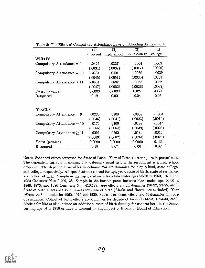
Table 5: The Effect of Compulsory Attendance Laws on Schooling Achievement(1)

drop out(2)

high school(3)

some college(4)

college+WHITESCompulsory Attendance = 9 -.0325 .0327 -.0004 .0003

(.0034) (.0037) (.0017) (.0020)Compulsory Attendance = 10 -.0331 .0401 -.0030 -.0039

(.0045) (.0051) (.0030) (.0033)Compulsory Attendance > 11 -.0551 .0582 -.0068 .0036

(.0047) (.0052) (.0026) (.0032)F-test (p-value) 0.0000 0.0000 0.027 0.171R-squared 0.12 0.02 0.04 0.05

BLACKSCompulsory Attendance = 9 -.0236 .0309 -.0069 -.0003

(.0046) (.0041) (.0023) (.0016)Compulsory Attendance = 10 -.0176 .0406 -.0182 -.0047

(.0065) (.0064) (.0039) (.0023)Compulsory Attendance > 11 -.0296 .0502 -.0189 .0016

(.0069) (.0062) (.0034) (.0025)F-test (p-value) 0.0000 0.0000 0.0000 0.136R-squared 0.19 0.07 0.06 0.02

Notes: Standard errors corrected for State of Birth Year of Birth clustering are in parentheses.The dependent variable in column 1 is a dummy equal to 1 if the respondent is a high schooldrop out. The dependent variables in columns 2-4 are dummies for high school, some college,and college, respectively. All specifications control for age, year, state of birth, state of residence,and cohort of birth. Sample in the top panel includes white males ages 20-60 in 1960, 1970, and1980 Censuses; N = 3,209,138. Sample in the bottom panel includes black males ages 20-60 in1960, 1970, and 1980 Censuses; N = 410,529. Age effects are 14 dummies (20-22, 23-25, etc.).State of birth effects are 49 dummies for state of birth (Alaska and Hawaii are excluded). Yeareffects are 3 dummies for 1960, 1970 and 1980. State of residence effects are 51 dummies for stateof residence. Cohort of birth effects are dummies for decade of birth (1914-23, 1924-33, etc.).Models for blacks also include an additional state of birth dummy for cohorts born in the Southturning age 14 in 1958 or later to account for the impact of Brown v. Board of Education.

4 0

Table 6: Are changes in compulsory attendance laws correlated with the number of policemen orstate police expenditures?

Number ofPolicemen

(1)

PoliceExpenditures

(2)

Per CapitaPolice Expend.

(3)Compulsory Attendance .9 .0024 .103 -.002

(.0080) (.186) (.002)Compulsory Attendance =10 -.0031 -.430 -.015

(0.0104) (.209) (.003)Compulsory Attendance =11 -.0080 .-340 -.011

(.0102) (.180) (.003)

R-squared 0.81 0.89 0.85343 1500 1500

Notes: Standard errors in parentheses. All specifications control for year and state effects. Thedependent variable in column 1 is the percentage policemen in the state. Sample in column 1includes observations from 49 states in years 1920, 1930, 1940, 1950, 1960, 1970, and 1980. Thenumber of policemen in 1920-40 are taken from Census reports on occupations and the laborforce for the entire U.S. population. Data from 1950-80 are from the IPUMS 1% Census samples.The dependent variable in column 2 is state police expenditures/$100 billions in constant dollars;Sample in column 2 includes observations from 49 states in all years from 1946 to 1978. Thedependent variable in column 3 is state per capita police expenditures in constant dollars; samplein column 3 includes observations from 49 states in years all years from 1946 to 1978. Data onpolice expenditures are from ICPSR 8706. See text for details.

4 1

Table 7: The Effect of Future Compulsory Attendance Laws on Current Graduation StatusWHITES BLACKS

Compuls.Att. = 9

(1)

Compuls.Att. = 10

(2)

Compuls.Att. >11

(3)

Compuls.Att. = 9

(4)

Compuls.Att. = 10

(5)

Compuls.Att.> 11

(6)

t = +4 -.0032 .0025 -.0141 .0054 -.0153 -.0164(.0122) (.0182) (.0214) (.0067) (.0110) (.0144)

t = +5 .0004 .0085 -.0007 -.0004 -.0098 -.0068(.0078) (.0113) (.0141) (.0046) (.0081) (.0101)

t = +6 .0006 .0100 .0027 -.0043 -.0132 -.0160(.0069) (.0093) (.0121) (.0045) (.0073) (.0095)

t = +7 .0001 .0107 .0027 -.0072 -.0136 -.0024(.0057) (.0078) (.0121) (.0043) (.0079) (.0090)

t = +8 .0013 .0106 .0091 -.0099 -.0106 -.0047(.0054) (.0071) (.0086) (.0042) (.0079) (.0083)

t = +9 .0016 .0092 -.0094 -.0126 -.0104 -.0060(.0051) (.0067) (.0080) (.0041) (.0079) (.0070)

t = +10 .0011 .0095 .0123 -.0140 -.0084 -.0041(.0046) (.0063) (.0071) (.0045) (.0078) (.0075)

t = +11 -.0013 .0063 .0131 -.0156 -.0071 -.0020(.0043) (.0055) (.0069) (.0049) (.0075) (.0078)

t = +12 -.0061 .0016 .0080 -.0158 -.0017 -.0042(.0047) (.0054) (.0072) (.0050) (.0070) (.0075)

t = +15 -.0092 -.0018 .00078 -.0097 .0122 -.0044(.0046) (.0054) (.0066) (.0052) (.0063) (.0079)

t = +18 -.0067 .0019 .0131 -.0020 .0271 -.0061(.0046) (.0055) (.0056) (.0055) (.0061) (.0085)

t = +20 -.0065 .0040 .0076 .0013 .0349 .0040(.0050) (.0060) (.0059) (.0064) (.0071) (.0083)

Notes: Standard errors corrected for State of Birth - Year of Birth clustering are in parentheses.The dependent variable is a dummy equal to 1 if the respondent is a high school graduate. Eachrow is a separate regression. All models control for compulsory attendance laws at t=0, t=1,t=2 and t=3, as well as year, age, state of birth, state of residence, and cohort of birth. Ageeffects are 14 dummies (20-22, 23-25, etc.). State of birth effects are 49 dummies for state of birth(Alaska and Hawaii are excluded). Year effects are 3 dummies for 1960, 1970 and 1980. Stateof residence effects are 51 dummies for state of residence. Cohort of birth effects are dummiesfor decade of birth (1914-23, 1924-33, etc.). Columns 4, 5, and 6 also include an additional stateof birth dummy for cohorts born in the South turning age 14 in 1958 or later to account for theimpact of Brown v. Board of Education. In column 1, 2 and 3, sample includes white males ages20-60 in 1960, 1970, and 1980 Censuses. In column 4, 5, and 6 sample includes black males ages20-60 in 1960, 1970, and 1980 Censuses. N = 3,209,138 for whites; N = 410,529 for blacks.

42

Table 8: The Impact of Years of Schooling on Incaceration Robustness ChecksWHITES BLACKS

OLS(1)

2SLS

(3)

OLS

(3)

2SLS(4)

(A) Base Case -.0010 -.0014 -.0037 -.0041(.00002) (.0006) (.0001) (.0019)

First Stage F-Test 36.2 41.5

(B) Region of Birth*Cohort Trend -.0010 -.0019 -.0037 -.0073(.00002) (.0010) (.0001) (.0026)

First Stage F-Test 12.79 28.39

(C) Region of Birth*Cohort Effects -.0010 -.0022 -.0037 -.0034(.00002) (.0017) (.0001) (.0035)

First Stage F-Test 5.74 22.41

(D) State of Birth*Cohort Trend -.0010 -.0034 -.0037 -.0067(.00002) (.0021) (.0001) (.0032)

First Stage F-Test 5.83 19.15

(E) Age Effects*Cohort Effects -.0010 -.0017 -.0037 -.0033(.00002) (.0007) (.0001) (.0023)

First Stage F-Test 37.90 35.68

(F) Education -.0015 -.0065 -.0087 -.0072(.0001) (.0014) (.0007) (.0063)

Education * Age .00002 .00007 .0001 .00003(.00000) (.00001) (.00001) (.00008)

Effect at Age 20 -.0011 -.005 -.006 -.006Effect at Age 40 -.0006 -.003 -.004 -.005First Stage F-Test 19.2-28.8 24.3-34.8

Notes: Standard errors corrected for state of birth - year of birth clustering are in parentheses.All specifications control for age, state of birth, and state of residence x year.

4 3

Table 9: OLS and IV Estimates of the Effect of Schooling on Arrest RatesOLS

(1) (2)

(A) AVERAGE EDUCATIONAvg. Years of Education -0.114 -0.116

(0.024) (0.023)R-squared 0.89 0.93

(B) HIGH SCHOOL GRADUATIONHS Graduation Rate -0.618 -0.674

(0.183) (0.181)R-squared 0.93 0.95

Controls:age x offense effects Y Yoffense x year effects y Yage x year effects Y ystate x age effects

Y Ystate x offense effects Ystate x year

2SLS(3) (4) (5) (6)

-0.111 -0.176 -0.182 -0.162(0.042) (0.080) (0.080) (0.105)

0.95

0.710 -0.946 -0.941 -0.873(0.283) (0.491) (0.522) (0.669)

0.96

Y Y Y Y

Y Y Y Y

Y y y Y

Y Y Y Y

Y Y Y

Y Y

Notes: Standard errors corrected for state-year-age clustering are in parentheses. The dependentvariable is the logarithm of the arrest rate by age, type of offense, state, and year. Averageschooling and high school graduation rate is by age group, state, and year (see text). All modelscontrol for percentage black. There are 8 age groups, 8 offenses, 50 states, and 4 years. All modelsare weighted by cell size.

4 4

Table 10: OLS Estimates for Arrest Rates by Type of CrimeAverage Educ. HS Grad. Rate

(1) (2) (3) (4)(A) VIOLENT vsViolent Crime

Property Crime

PROPERTY CRIME-.121 -.116 -.751(.025) (.044) (.198)-.111 -.105 -0.593(.026) (.044) (.208)

(B) BY DETAILED TYPE OF CRIME

-.793(.291)-0.621(.304)

Murder -.276 -.274 -2.062 -2.133(.041) (.058) (.403) (.403)

Rape .113 .118 1.094 1.049(.037) (.048) (.307) (.353)

Robbery -.007 -.005 0.184 0.113(.031) (.047) (.253) (.333)

Assault -.297 -.292 -2.136 -2.179(.028) (.048) (.226) (.326)

Burglary -.057 -.052 -0.202 -0.250(.032) (.048) (.268) (.347)

Larceny -.058 -.052 -0.235 -0.277(.027) (.045) (.209) (.311)

Vehicle Theft -.201 -.197 -1.227 -1.271(.030) (.048) (.251) (.346)

Arson -.133 -.127 0.745 -0.784(.044) (.053) (.358) (.408)

Additional Controls:state x year

Notes: Standard errors corrected for state-year-age clustering are in parentheses. Violent crimesinclude murder, rape, robbery, and assault. Property crimes include burglary, larceny, vehicletheft, and arson. Average schooling and high school graduation rate are by age group, state, andyear (see text). All specifications control for percentage black, age x offense effects, offense x yeareffects, age x year effects, state x age effects and state x offense effects. There are 8 age groups,8 offenses, 50 states, and 4 years. All models are weighted by cell size.

Table 11: The Effect of Education on Self-Reported Crime and Incarceration for Whites (NLSY)Years of School HS Graduate(1) (2) (3) (4)

Self-Reported CrimeViolent Crime -0.0212 -0.0177 -0.1063 -0.1102

(0.0078) (0.0087) (0.0218) (0.0229)Drug Sales -0.0151 -0.0156 -0.0562 -0.0555

(0.0054) (0.0060) (0.0153) (0.0159)Property Crime -0.0184 -0.0151 -0.1155 -0.1259

(0.0111) (0.0122) (0.0311) (0.0321)Any Crime 70.0310 -0.0287 -0.1627 -0.1758

(0.0122) (0.0135) (0.0341) (0.0355)

Incarcerated -0.0053 -0.0056 -0.0331 -0.0315(0.0005) (0.0007) (0.0027) (0.0032)

Controls:Age/Cohort y y y YRegion of Residence

Y y y YEnrolled in School Y Y Y YFamily Background

Y YAbility y YSMSA Status y YLocal Unemployment Rate y YState Incarceration Rate

Y Y

Notes: Self-reported crimes are based on men ages 18-23 in 1980. Violent crimes correspond torobbery and assault, while property crimes include shop-lifting and all other thefts of over $50.Each row represents a separate OLS regression. The dependent variables for the self-reportedcrimes are dummy variables equal to one if the person participated in that type of crime; infor incarceration, it is a dummy equal 1 if the individual was incarcerated at any time overages 22-28. The reported coefficients for incarceration are obtained by adjusting the ages 22-28incarceration rates by the ratio of the probability of incarceration for the seven year span to theannual incarceration probability (over those same ages). Family background measures include:current enrollment in school, parents highest grade completed, whether or not the individual livedwith both of his natural parents at age 14, whether his mother was a teenager at his birth, andfamily income.

4 6

Tab

le 1

2: S

ocia

l Cos

ts p

er C

rim

e an

d So

cial

Ben

efits

of

Incr

easi

ng H

igh

Scho

ol C

ompl

etio

nR

ates

by

1%

Vic

tim C

osts

per

crim

e(1

)

Prop

erty

Los

spe

r cr

ime

(2)

Inca

rc. C

ost

per

crim

e(3

)

Tot

al C

ost

per

crim

e(4

)

Est

. Cha

nge

in A

rres

ts(5

)

Est

. Cha

nge

in C

rim

es(6

)

Soci

al B

enef

it(4

) x

(6)

(7)

Vio

lent

Cri

mes

Mur

der

2,94

0,00

012

084

5,45

53,

024,

359

-373

-373

$1,1

29,5

96,5

62R

ape

87,0

0010

02,

301

89,2

2134

71,

559

-$13

9,10

9,27

8R

obbe

ry8,

000

750

1,98

59,

385

134

918

-$8,

617,

191

Ass

ault

9,40

026

538

9,91

7-7

,798

-37,

135

$368

,252

,227

Prop

erty

Cri

mes

Bur

glar

y1,

400

970

363

987

-653

-9,4

67$9

,342

,643

Lar

ceny

/The

ft37

027

044

198

-1,9

83-3

5,10

5$6

,944

,932

Mot

or V

ehic

le T

heft

3,70

03,

300

185

1,24

5-1

,355

-14,

238

$17,

728,

056

Ars

on37

,500

15,5

001,

542

39,0

42-6

9-4

69$1

8,32

3,74

8

Tot

al11

,750

94,3

10$1

,402

,461

,698

Not

es: V

ictim

cos

ts a

nd p

rope

rty

loss

es ta

ken

from

Tab

le 2

of

Mill

er, C

ohen

, and

Wie

rsem

a(1

996)

. Inc

arce

ratio

n co

sts

per

crim

e eq

ual

the

inca

rcer

atio

n co

st p

er in

mat

e, $

17,0

27 (

Step

han

1999

), m

ultip

lied

by th

e in

carc

erat

ion

rate

(L

ynch

et a

l. 19

94).

Tot

al c

osts

are

calc

ulat

ed a

s th

e su

m o

f vi

ctim

cos

ts a

nd in

carc

erat

ion

cost

s le

ss 8

0% o

f th

epr

oper

ty lo

ss (

alre

ady

incl

uded

in v

ictim

cos

ts)

for

all c

rim

esex

cept

ars

on. T

otal

cos

ts f

or a

rson

are

the

sum

of

vict

im c

osts

and

inca

rcer

atio

nco

sts.

See

text

for

det

ails

. Est

imat

ed c

hang

e in

arr

ests

calc

ulat

ed f

rom

pan

el B

, col

umn

4 of

Tab

le 1

0 an

d th

e to

tal n

umbe

r of

arr

ests

in19

90 U

nifo

rm C

rim

e R

epor

ts. E

stim

ated

cha

nges

incr

imes

adj

usts

the

arre

st e

ffec

t by

the

num

ber

of c

rim

espe

r ar

rest

. The

soc

ial b

enef

it is

the

estim

ated

cha

nge

in c

rim

es in

col

umn

6tim

es th

e to

tal c

ost p

er c

rim

e in

col

umn

4. A

ll do

llar

figu

res

are

in 1

993

dolla

rs. S

ee te

xt f

or d

etai

ls.

4 8

Appendix A Interpretation of IV and OLS Estimators

When estimating the impact of high school graduation on the probability of incarceration using

only an indicator variable for graduation status, OLS and IV estimators can be written as weighted

sums of causal responses to each unit change in schooling (i.e. completing grades 9, 10, 11,

12, etc.), where the sets of "weights" differ for the two estimators. The results presented here

build on Angrist and Imbens (1995) to show that the "weights" placed on the effects of each

schooling progression have an intuitive interpretation and are functions of observable quantities.

The expected difference between the estimators depends on the difference in the weights as well

as the impacts of schooling on incarceration at each grade level. In our context, we empirically

show that differences in these "weights" explain much of the difference between our OLS and IV

estimates for blacks.

Consider the following model for incarceration: yj(s) = E oj + Ei , which depends on the levelj=o

of schooling s E {1, 2, ..., S} and a mean zero individual-specific iid error term ei (all individuals

are assumed to have the same 0's).37 Let D be an indicator equal to one when s > k and zero

otherwise. In our case, k = 12, so D represents high school graduation. For purposes of this

analysis, assume that D is independent of e. The OLS regression

yi = + 0Di + ei (3)

yields an estimate for 0 with

k-1plim ijoLs = E(yls k) E(yls < k) = Ok E E (4)

j=1 j=k+1

where 03 = Pr(s < jis < k) and 03 = Pr(s > js > k). OLS estimates of the 03's are pictured inFigure 1.

Consider an instrument Z E {0, 1, 2, ..., /} that satisfies the monotonicity and independence

assumptions of Angrist and Imbens (1995).38 The two stage least squares (2SLS) estimate for 0

using / indicator variables (zi = 1 if Z = i and zero otherwise) as instruments for D in equation

(3) has

where

Ely[E(DIZ) E(D)11phrit 432SLS

EfE(DIZ)[E(DIZ) E(D)]} AA'jOk

Pr(Z = i)[E(DIZ = i) E(D)]Pr(si > j > so)= i=1

Pr(Z = i)[E(DIZ = i) E(D)]Pr(si k > so)j=1

(5)

(6)

37For a discussion of IV estimation and random coefficient models, see Heckman (1997), Heckman and Vytlacil(2001), and Imbens and Angrist (1994).

38In our case, Z=0 if compulsory schooling is 8 years or less; Z=1 if compulsory schooling is 9 years; Z=2 ifcompulsory schooling is 10 years; Z=3 if compulsory schooling is 11 or 12 years.

4 9

and .3, is the schooling choice for someone when Z = z. The A-weights depend on the number of

individuals whose education level is affected by each of the instruments (Pr(si > j > so)) and the

distance between E(D1Z = i) and E(D).39 Equations (4) and (5) show that the OLS and 2SLS

estimators are different weighted sums of the causal responses to each unit change in schooling.

Although we refer to the O's, O's, and A's as "weights" for lack of a better word, neither the OLS

nor the 2SLS "weights" sum to 1. For both OLS and 2SLS estimators, the weights on 012 alone

must equal one, so their sums will generally be greater than one.

In general, the OLS and 2SLS estimates need not coincide even if OLS estimates are not

plagued by endogeneity problems. This is because both estimators estimate different functions of

the underlying O's. Comparing the 2SLS and OLS estimates produces the following relationship:

k-1plim (I2sLs ijoLs) = E(A i-0,),51,+ E (A,- 03)133.

j=1 j=k+1(7)

Equation (7) makes clear that only special cases will yield OLS and 2SLS estimates with the

same expectation.° The empirical values for these weights are shown in Figure A-1, separately

for blacks and whites. While the difference in 2SLS and OLS weights is small for whites, it issizeable for blacks.

Recall that the OLS estimates for blacks are smaller than the 2SLS estimates despite the fact

that endogeneity would lead us to expect the opposite. Both OLS and 2SLS estimates are similar

for whites. Do the weights explain these findings? Re-weighting the OLS estimates of each causal

response (as shown in Figure 1) by the 2SLS weights in Figure A-1 produces an adjusted impact

of 0.0077 for whites and 0.05 for blacks. While re-weighting the OLS estimator produces little

change for whites (when compared with the OLS estimates in Table 4), it substantially increases

the estimated effect for blacks. This is consistent with what we observe for the 2SLS estimates

in the table. Although this evidence is only suggestive, the larger 2SLS estimates for blacks seem

to reflect, at least in part, the differences in weights that OLS and 2SLS give to the impacts

of different schooling levels on crime. Some of the 2SLS-OLS difference may also be attributed

to their imprecision. Using a standard Hausman test, we cannot reject that the OLS and 2SLS

estimates are the same for both whites and blacks.

We now turn to the model that is linear in years of schooling. In this case, the 2SLS estimators

of the coefficient on years of schooling equals E A3,3i, and the OLS estimator equals E3=1 J=1

39See Appendix A of Lochner and Moretti (2001) for a derivation of these A-weights.49There are two such special cases. First, schooling may have no effect on incarceration at any level except

moving from 11 to 12 years. In this case, )33 = 0 for all j 12, and the two estimators consistently estimate theeffect of moving from 11 to 12 years of school. Second, A, = 0, for all j < 12 and A, = 03 for all j > 12. In thisunlikely event, both estimators will yield the same weighted sums of all causal effects.

50

The 2SLS weights are

Pr(Z = i)IE(.91Z = i) E(s))Pr(si j > so)= I

E Pr(Z = i)[E(sIZ = i) E(s)][E(siZ = i) E(sIZ = 0)]i=1

The OLS weights are wi = [Pr(s > j)(E(sls > j) E(s))[IVar(s). For a detailed discussion ofOLS weights in a continuous regressor context, see Yitzhaki (1996). Unlike the previous weights,

sthese 2SLS and OLS weights must sum to one: E = E Lei = 1. They are weighted averages

j=1 j=1of all causal impacts, where the weights are shown in Figure A-2. The differences between OLSand 2SLS weights are small for both blacks and whites, consistent with the small difference inpoint estimates based on the linear specification shown in Table 3.

Finally, we turn to the effect of moving from 11th grade to 12th grade. If the relationshipbetween education and incarceration is non-linear as suggested by Figure 1, what do our 2SLSestimates say about the impact of completing high school (i.e. moving from 11th grade to 12thgrade)? As discussed above, the 2SLS estimator using an indicator for high school graduationwill over-estimate this effect. On the other hand, if the effect of completing 12th grade is greaterthan the impact of any other single-year grade transition, the linear-in-schooling 2SLS estimatorwill under-estimate the effect of finishing the 12th grade since it is a weighted average of allsingle-year causal effects. Thus, the effect of finishing 12th grade should be bounded by thelinear-in-schooling and the graduate dummy specifications.

511.

Figure A-1: 2SLS and OLS Weights for the Model that Includes a Dummy for HS Graduate

WHITES

TWOSLS- differ OLS

9 12educ

Years of Schooling

BLACKS

TWOSIS- differ OLS

9 12educ

Years of Schooling

Figure A-2: 2SLS and OLS Weights for the Model Linear in Years of Schooling

WHITES

TWOSLS OLSDIFF

A 6 1'2educ

Years of Schooling

BLACKS

TWOSLSDIFF

01.S

18

3 6 9 12 15 18

Years of Schooling

The lines with circles plot 2SLS weights for each year of schooling; the lines with triangles plot

OLS weights. The lines with '+' plot the difference between 2SLS and OLS weights.

U.S. Department of EducationOffice of Educational Research and Improvement (OERI)

National Library of Education (NLE)Educational Resources Information Center (ERIC)

REPRODUCTION RELEASE(Specific Document)

I. DOCUMENT IDENTIFICATION:

t)O 03`1011

ERIC

e of E. QczL4ov o Cv wte E v cieC.Q "ipv,-;10

Acr ests 0.(kA Si ç `P-Q-f tAsAuthor(s): Lax,c_e_ LockAdle-

UAW cvs ck-.) 0 t- Qockesi-ti.

ULC-1 (_ ez,r- ekkN)

Title:

Corporate Source: Publication Date:

II. REPRODUCTION RELEASE:In order to disseminate as widely as possible timely and significant materials of interest to the educational community, documents announced in the

monthly abstract journal of the ERIC system, Resources in Education (RIE), are usually made available to users in microfiche, reproduced paper copy,and electronic media, and sold through the ERIC Document Reproduction Service (EDRS). Credit is given to the source of each document, and, ifreproduction release is granted, one of the following notices is affixed to the document.

If permission is granted to reproduce and disseminate the identified document, please CHECK ONE of the following three options and sign at the bottomof the page.

The sample sti:ker shown beiow will beaffixed to all Level 1 documents

PERMISSION TO REPRODUCE ANDDISSEMINATE THIS MATERIAL HAS

BEEN GRANTED BY

TO THE EDUCATIONAL RESOURCESINFORMATION CENTER (ERIC)

Check here for Level 1 release, permittingreproduction amd dissemination in microfiche or other

ERIC archival media (e.g., electronic) and papercoPY.

Signhere,-)please

lbe sample sticker shown below will beaffixed to all Level 2A documents

PERMISSION TO REPRODUCE ANDDISSEMINATE THIS MATERIAL IN

MICROFICHE, AND IN ELECTRONIC MEDIAFOR ERIC COLLECTION SUBSCRIBERS ONLY,

HAS BEEN GRANTED BY

TO THE EDUCATIONAL RESOURCESINFORMATION CENTER (ERIC)

2A

Level 2A

Check here for Level 2A release, permittingreproduction and dissemination in microfiche and in

electronic media for ERIC archival collectionsubscribers only

The sample sticker shown below will beaffixed to all Level 28 documents

PERMISSION TO REPRODUCE ANDDISSEMINATE THIS MATERIAL IN

MICROFICHE ONLY HAS BEEN GRANTED BY

2B

TO THE EDUCATIONAL RESOURCESINFORMATION CENTER (ERIC)

Level 28

LICheek here for Level 28 release, permitting

reproducfion and dissemination in microfiche only

Documents will be processed as Indicated provided reproduction quality permits.tf permission to reproduce is granted, but no box Is checked, documents will be processed at Level 1.

I hereby grant to thi Educational Resources Information Center (ERIC) nonexclusive permission to reproduce and disseminate this documentas indicated above. Reproduction from the ERIC microfiche or electronic media by persons other than ERIC employees and its systemcontractors requires permission from the copyright holder. Exception is made fornon-profit reproduction by libraries and other senfice agenciesto satisfy information needs of educators in response to disaete inquiries

laturegan;-ZEZ'°'r'P----Th

Rood Name/Position/Tit* L &Ace Le, /iks.515rtak.Af Tre.-{csso

C

N Y 146.)7 '

Tetro 3- 030E-Mall Aftess:

FAX 65 7a3-16g7°ate 02-lef'0?-

1,A.A>cc rgoi_cc . RocitegreP-t-D LA. (over)

III. DOCUMENT AVAILABILITY INFORMATION (FROM NON-ERIC SOURCE):

If permission to reproduce is not granted to ERIC, or, if you wish ERIC to cite the availability of the document from another source, pleaseprovide the following information regarding the availability of the document. (ERIC will not announce a document unless it is publiclyavailable, and a dependable source can be specified. Contributors should also be aware that ERIC selection criteria are significantly morestringent for documents that cannot be made available through EDRS.)

Publisher/Distributor:

Address:

Price:

IV. REFERRAL OF ERIC TO COPYRIGHT/REPRODUCTION RIGHTS HOLDER:

If the right to grant this reproduction release is held by someone other than the addressee, please provide the appropriate name andaddress:

Name:

Address:

V. WHERE TO SEND THIS FORM:

Send this form to the following ERIC Clearinghouse:Acquisitions Coordinator

ERIC Clearinghouse on Adult, Career, and Vocational EducationCenter on Education and Training for Employment

1900 Kenny RoadColumbus, OH 43210-1090

However, if solicited by the ERIC Facility, or if making an unsolicited contribution to ERIC, return this form (and the document beingcontributed) to:

4,1

EFF-088 (Rev. 2/2000)