Finance and Economics Discussion SeriesDivisions of Research & Statistics and Monetary Affairs

Federal Reserve Board, Washington, D.C.

Research and development, profits and firm value: A structuralestimation

Missaka Warusawitharana

2008-52

NOTE: Staff working papers in the Finance and Economics Discussion Series (FEDS) are preliminarymaterials circulated to stimulate discussion and critical comment. The analysis and conclusions set forthare those of the authors and do not indicate concurrence by other members of the research staff or theBoard of Governors. References in publications to the Finance and Economics Discussion Series (other thanacknowledgement) should be cleared with the author(s) to protect the tentative character of these papers.

Research and Development, Profits and Firm Value:

A Structural Estimation

Missaka Warusawitharana∗

Board of Governors of the Federal Reserve System

Abstract

Is the return to private R&D as high as believed? This study identifies a flaw in the production

function approach to estimating the return to R&D. I provide new estimates based on a structural

estimation approach that incorporates uncertainty about the outcome from R&D. The results

shed light on the rate of innovation, the impact of an innovation on profits, and the market value

of the R&D stock. The parameter estimates imply a mean return to R&D of 3.7-5.5%, much

lower than previous values. The analysis also demonstrates the unsuitability of using the return

to R&D as a basis for policy decisions on tax subsidies to R&D.

September 16, 2008

∗I thank Marco Cagetti, John Fernald, Joao Gomes, Jonathan Heathcote, Michael Palumbo, Simon Gilchristand seminar participants at the 2008 Econometric Society Summer meetings, the 2008 SED meetings and theFederal Reserve Board for valuable comments and suggestions. The views expressed in this paper are mine anddo not reflect the views of the Board of Governors of the Federal Reserve System or its staff. Contact: Divisionof Research and Statistics, Board of Governors of the Federal Reserve System, Mail Stop 97, 20th Street andConstitution Avenue NW, Washington, DC 20551. m1mnw00@frb.gov, (202)452-3461.

1 Introduction

Estimating the returns to research and development (R&D) expenditures has value from an eco-

nomic growth perspective (Romer (1990)) and a macro fluctuations perspective (Comin and Gertler

(2006) and Barlevy (2007)). A substantial literature employs the production function based ap-

proach of Griliches (1979) and finds returns to private R&D in the range of 25 - 60%. Based partly

on this finding, Jones and Williams (1998) argue that optimal R&D investment is two to four times

the observed level. However, is the return to R&D as high as believed and should the return be

used as a basis for policy decisions?

This study begins by demonstrating that the production function approach to estimating the

return to R&D suffers from an indeterminacy flaw: the estimated returns vary sharply with the

assumed obsolescence rates. The production function approach estimates the elasticity of value-

added with respect to R&D using regressions of log value-added on factor inputs. This literature

finds that different obsolescence rates lead to similar elasticity estimates. Therefore, the literature

focuses on the estimates obtained assuming an obsolescence rate of 15%, as in Griliches and Mairesse

(1984). However, the estimated next period return equals the elasticity estimate times the ratio of

value-added to R&D stocks, which varies with the obsolescence rate. Thus, different assumptions

for the obsolescence rate lead to different estimates for the return to R&D.

This study tackles the above problem by using structural estimation to estimate the return to

R&D.1 The underlying model incorporates uncertainty in the outcome to R&D, unlike the produc-

tion function approach. Such uncertainty is arguably a key economic feature of R&D investment as

neither researchers nor managers know the outcome of an R&D project when they initiate it. The

model incorporates uncertainty from R&D in a manner similar to the endogenous growth literature

(Romer (1990), Grossman and Helpman (1991), and Aghion and Howitt (1992)) by assuming that

the R&D stock impacts the probability of an innovation, which results in higher profits in the

future. The model thus departs from the production based literature, which treats R&D stocks as

simply another input in the production function.

The model economy consists of firms in an R&D sector and non-R&D sector. This follows the

Compustat data set as most firms either report positive R&D for all years or report no R&D at all.

Firms in the non-R&D sector are modelled following the Q-theoretic approach, with a downward

sloping demand curve (Gomes (2001) and Eberly, Rebelo, and Vincent (2008)). In addition to

1Other papers which use this method include: Cooper and Ejarque (2003); Hennessy and Whited (2005); Cooperand Haltiwanger (2006); Hennessy and Whited (2007); Bloom (2008); and Eberly, Rebelo, and Vincent (2008).

1

physical investment, firms in the R&D sector also accumulate an R&D stock. The R&D stock

does not reflect the stock of ideas applicable for production, as in Griliches (1979). Instead, the

R&D stock measures the degree of investments made by the firm towards generating the next

innovation. In each period, a firm may successfully innovate, leading to a jump in the firm’s profits

that dissipates over time. Prior innovations by the firm are reflected in the current profitability

level. A firm would realize a negative return from R&D investment in a year in which it failed to

innovate, thereby enabling the model to capture failed R&D outcomes.

The model yields an explicit characterization of the R&D policy function in terms of the ex-

pected increase in firm value from an innovation and the residual value of R&D investment in the

next period. An unexpected feature of the model is that the optimal R&D policy does not neces-

sarily increase with the return. The return to R&D measures the increase in next period profits

from an innovation, which is only one aspect of the impact of R&D on firm value, which determines

optimal R&D investment. Parameter changes can simultaneously yield higher returns to R&D and

lower optimal R&D investment.

Identification of the model parameters follows from matching moments on R&D, profits, and

valuations for both R&D and non-R&D sector firms. The estimates reveal that an innovation leads

to increases in profitability of 13% to 19%. The fraction of firms innovating each year ranges from

0.41 to 0.51. These estimates indicate that firms generate a substantial increase in profits from

an innovation but also face significant uncertainty on the outcome of their R&D investments. The

estimated mean annual return to private R&D ranges from 3.7% to 5.5%, much lower than the

production function estimates. These low returns are partly explained by a high autocorrelation

term that implies the benefit of an innovation lasts many periods into the future. The low returns

do not, however, deter firms from generating the high R&D investment levels observed in the data.

The model also enables an estimation of the market value of the R&D stock. Hall (2001)

highlights the growing importance of intangible capital in the US economy. The estimates indicate

that the market value of R&D stocks as a fraction of all capital ranges from 16.7% to 23.1%.

Combined with the high level of R&D investment, this demonstrates the prominent role of R&D

in understanding capital accumulation.

Counterfactual experiments on a additional 5% tax subsidy to R&D generate economically

significant increases in R&D investment and the rate of innovation for all the estimated models.

This demonstrates that the low return to R&D does not invalidate prior arguments for robust

policy actions in favor of R&D investment, particularly given the evidence of technology spillovers

2

found by Bloom, Schankerman, and van Reenen (2007). Taken together, these results demonstrate

that the return to R&D is much lower than commonly believed and should not be used for forming

R&D related policy decisions.

2 Model

The model economy consists of a large number of heterogeneous firms. The firms operate in either

an R&D sector or a non-R&D sector. The two sectors differ only in that firms in the R&D sector

can engage in R&D and potentially obtain an improvement in their profitability while firms in the

non-R&D sector cannot do so. Firms are exogenously assigned to each sector and do not switch

from one to another (see Klette and Kortum (2004) for a model where firms endogenously decide

whether to engage in R&D or not). These assumptions correspond to the data on US firms, where

some firms report positive R&D activity for most or all periods and others report zero R&D for all

periods. The model does not incorporate leverage.

2.1 The non-R&D sector

Non-R&D firms operate as standard Q-theory firms facing a downward sloping demand curve.2 In

each period, the output of the ith firm follows a Cobb-Douglas specification with

Y (Ki, xi) = xiKνi L1−ν

i ,

where ν denotes the elasticity of output with respect to capital (time subscripts omitted). The firm

faces a downward sloping demand curve

Pi = diY−ηi ,

where d denotes a demand shift parameter and η equals a constant price elasticity term. Assuming

a deterministic wage process and a per period fixed cost of operations c, the profits of the firm can

be written as

Π(Ki, zi) = ziKθi − c,

2See Gomes (2001), Bloom (2008), and Eberly, Rebelo, and Vincent (2008).

3

where zi inherits the properties of xi, and the decreasing returns to scale parameter θ is a function

of η and ν. The subsequent analysis employs the above profit function. The firm spends its profits

on capital investments and returns any cash left as a dividend to shareholders, with negative divi-

dends indicating a share issuance. Both investment and disinvestment activity incurs a symmetric

quadratic adjustment cost, and firms can freely disinvest.3 The capital stock of the firm in the next

period is given by

K ′

i = Ki(1 − δ) + Ii,

where δ denotes the depreciation rate and Ii equals investment. The per period dividend of the

firm equals

Dn(Ki, zi) = Π(Ki, zi)(1 − τn) − Ii − bI2i

2Ki, (1)

where b measures the level of quadratic adjustment costs for physical capital and τn denotes a linear

tax rate on operating profits.4 Taxes drive a wedge between operating profits and firm values. The

above specification enables the model to incorporate this wedge in a parsimonious manner. The

transition equation for log profitability follows an AR(1) process with

log(z′i) = µ + ρ log(zi) + εi (2)

εi ∝ N(0, σ2).

The parameters of the above process are identical across firms in the non-R&D sector. Thus,

heterogeneity across firms is driven by heterogeneity in shocks to profitability. Let β < 1 denote

the discount factor. Given these assumptions, the value of the firm can be obtained as the solution

to a Bellman equation:

V n(Ki, zi) = maxIi,K

′

i

Dn(Ki, zi) + βEz[Vn(K ′

i, z′

i)], (3)

K ′

i = Ki(1 − δ) + Ii.

3For simplicity, the model does not include any irreversibility of selling physical capital as in Abel and Eberly(1994) or any costs of external finance as in Brown, Fazzari, and Petersen (2008). Including these frictions wouldlikely have no significant impact on the R&D parameter estimates of interest while substantially complicating themodel solution and estimation.

4Superscripts n and r denote the non-R&D and R&D sectors, respectively.

4

The results given in Stokey and Lucas (1989, Chapter 9) ensure the existence and uniqueness of

V n(Ki, zi) and the policy function Ii.

2.2 The R&D sector

Firms in the R&D sector are similar to those in the non-R&D sector, except for their R&D activity.

These firms also invest in a stock of R&D. The R&D stock of the firm does not directly impact

the production function as in Griliches (1979) and others. Instead, the R&D stock stochastically

affects the transition of profitability across periods. The model views R&D stocks as measuring

the potential for future innovations rather than a measure of the stock of ideas applicable for

production. When a firm’s R&D activity is successful, the firm realizes a profitability jump in the

next period.5 If the R&D effort was not successful, the firm will not realize a jump in profitability.

These innovations reflect discoveries by firms that lead to an increased profitability of the firm’s

capital stock.6 A fraction of the R&D stock becomes obsolete each period reflecting the conclusion

or abandonment of R&D projects. The model attempts to capture the inherently uncertain nature

of the innovation process through this mechanism as a firm would realize a negative return from

its R&D investment in a year in which it failed to innovate.

Denote the accumulated R&D stock of the firm at the end of each period by S′

i. Let Ri equal

the investment in R&D activity. The law of motion for R&D stocks is given by

S′

i = Si(1 − γ) + Ri, (4)

where γ denotes the rate at which R&D stocks become obsolete. Let ji denote a binary variable

that equals 1 if the firm successfully innovates, and 0 otherwise. The probability of a successful

innovation is given by a Bernoulli distribution with success probability

p(ji = 1) = 1 − exp(−aS′

i

Ki), (5)

where a is a parameter that influences the success rate of innovations. Higher R&D stocks lead

to a greater probability of a successful innovation. This particular parametrization implies that

5Other papers which provide a similar treatment of the innovation process include Klette and Kortum (2004),Aghion, Bloom, Blundell, Griffith, and Howitt (2005), and Li (2007).

6The vintage capital models of Greenwood and Jovanovic (1999) and Hobijn and Jovanovic (2001) emphasizemacro level technological revolutions that have different impacts on the value of current and future capital.

5

success probabilities are concave in S′

i. The success probability decreases as the current capital

stock increases. The scaling by capital stock can be thought of as capturing an increase in R&D

project size with firm size. As such, larger firms require a greater level of R&D investment to

generate the same probability of success as a small firm. The scaling ensures that large firms do

not benefit disproportionately from R&D activity.7 In the event of success, log profitability jumps

by a constant λ.8 This measures the improvement in the firm’s profitability from a successful

innovation. The transition equation for profitability of firms in the R&D sector is as follows:

log(z′i) = µ + ρ log(zi) + λji + εi (6)

ji ∝ B(p(S′

i

Ki)) (7)

εi ∝ N(0, σ2),

The distribution for ji is independent of the distribution for εi. In this setup, the transition

equation for profitability becomes an AR(1) process with jumps, where the jump intensity varies

endogenously with R&D stocks.

The model is agnostic on the source of the jump in profits from a successful innovation. This

may arise from either improvements in the current products of the firm, the introduction of entirely

new products, or cost reductions. More formally, a successful innovation may result in an increase

in the productivity parameter xi or the demand shifter d. The model does not take a stand on

whether patent protection is necessary for generating an increase in profitability (see Boldrin and

Levine (2008)). While the inability to link R&D investment directly to total factor productivity

may be a drawback, the above approach has the benefit of allowing R&D to have a broader impact.

Correspondingly, the endogenous growth literature highlights both quality improvements and new

product introductions as the outcome of innovations.

The timing of the firm’s decisions warrant clarification. R&D sector firms enter each period

with an R&D stock, a capital stock, and a profitability level. The firms invest in R&D and capital

during the period. At the end of the period, each firm discovers whether it successfully innovated

7The endogenous growth theory model of Romer (1990) implies that innovation increases in the level of R&D.Subsequent work by Jones (1995b) demonstrates that this relationship does not hold in the data. Jones (1995a),Young (1998), and Segerstrom (1998) introduce endogenous growth models without scale effects. In the currentmodel, a lack of scaling leads to explosive value functions as large firms will continue to increase R&D spending andincrease their probability of success.

8Kortum (1997) employs a search theoretic approach, in which the rate of arrival of ideas is exogenous and theefficiency of the improvement depends on the R&D stock.

6

or not. If a firm succeeds, its next period profitability will be higher than if it did not. The

accumulated R&D stock carries over to the next period and a fraction of it becomes obsolete after

the realization of the profitability level z′. Note that this timing sequence differs from the law of

motion for capital: the current period R&D investment adds to the R&D stock which impacts the

realization of the next profitability level. This timing structure was chosen as it yields a value

function that is separable in the R&D stock. It also captures the idea that R&D investment in the

current period impacts the firm’s profitability in the next period.

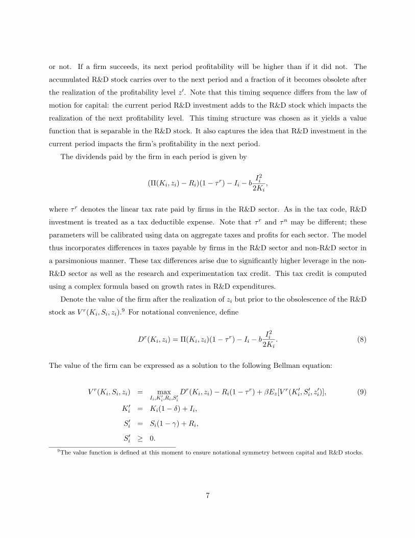
The dividends paid by the firm in each period is given by

(Π(Ki, zi) − Ri)(1 − τ r) − Ii − bI2i

2Ki,

where τ r denotes the linear tax rate paid by firms in the R&D sector. As in the tax code, R&D

investment is treated as a tax deductible expense. Note that τ r and τn may be different; these

parameters will be calibrated using data on aggregate taxes and profits for each sector. The model

thus incorporates differences in taxes payable by firms in the R&D sector and non-R&D sector in

a parsimonious manner. These tax differences arise due to significantly higher leverage in the non-

R&D sector as well as the research and experimentation tax credit. This tax credit is computed

using a complex formula based on growth rates in R&D expenditures.

Denote the value of the firm after the realization of zi but prior to the obsolescence of the R&D

stock as V r(Ki, Si, zi).9 For notational convenience, define

Dr(Ki, zi) = Π(Ki, zi)(1 − τ r) − Ii − bI2i

2Ki. (8)

The value of the firm can be expressed as a solution to the following Bellman equation:

V r(Ki, Si, zi) = maxIi,K

′

i,Ri,S

′

i

Dr(Ki, zi) − Ri(1 − τ r) + βEz[Vr(K ′

i, S′

i, z′

i)], (9)

K ′

i = Ki(1 − δ) + Ii,

S′

i = Si(1 − γ) + Ri,

S′

i ≥ 0.

9The value function is defined at this moment to ensure notational symmetry between capital and R&D stocks.

7

The lack of a non-negativity constraint on R&D investment implies that firms can sell their R&D

if necessary. While firms do so infrequently in the simulation, this assumption is necessary for

the subsequent characterization of the R&D policy function. The reversibility assumption is also

supported by anecdotal evidence of firms selling partially developed products to other firms, partic-

ularly in the pharmaceutical sector. The expectation in the Bellman equation is taken over the joint

distribution for ji, εi. The results in Bertsekas (2000, Chapter 7) yield the existence and uniqueness

of the solution to the above problem. Substituting the expression for Ri into the maximization

problem yields

V r(Ki, Si, zi) = maxIi,K

′

i,S′

i

Dr(Ki, zi) + Si(1 − γ)(1 − τ r) − S′

i(1 − τ r) + βEz[Vr(K ′

i, S′

i, z′

i)],

K ′

i = Ki(1 − δ) + Ii,

S′

i ≥ 0.

Observe that Si does not impact the optimization problem for either K ′

i or S′

i. This motivates the

conjecture that the value of the firm can be simplified as follows:

V r(Ki, Si, zi) = G(Ki, zi) + Si(1 − γ)(1 − τ r). (10)

The value of the R&D stock equals Si(1 − γ)(1 − τ r) due to the model’s timing convention. The

value function is defined after the realization of zi, but before the anticipated obsolescence of the

R&D stock at the beginning of the period. Thus, the effective value of Si equals its value after

obsolescence, which is reduced by the tax deductability of R&D expenditures. Substituting the

above expression into the Bellman equation, one obtains:

G(Ki, zi) = maxIi,K

′

i,S′

i

Dr(Ki, zi) − S′

i(1 − τ r) + βS′

i(1 − γ)(1 − τ r) + βEz[G(K ′

i, z′

i)], (11)

K ′

i = Ki(1 − δ) + Ii,

S′

i ≥ 0.

This establishes our conjecture and demonstrates that the value function is separable in the R&D

stock. Note that this is not a general result, and it arose from the particular assumptions made

about the timing and structure of the optimization problem. The separability ensures that the

8

return to R&D investment is negative in periods where the firm does not innovate.

2.3 R&D policy

The above analysis simplifies the solution of the optimal R&D policy of the firms. The optimal

choice of S′

i impacts the current period dividend payment, the level of R&D stock carried over to

the next period, as well as the transition equation for profitability z. The first two pieces are linear

in S′

i. Let S′

i be the optimal policy in the interior region, where the S′

i ≥ 0 constraint does not

bind. The following proposition characterizes the optimal R&D stock in this region:

Proposition 1 The optimal R&D stock of the firm when S′

i > 0 is given by

S′

i

Ki=

1

a

[

log(a) − log ((1 − τ r)(1 − β(1 − γ))) + log

(

β(Ez[G(K ′

i, z′

i)|ji = 1] − Ez[G(K ′

i, z′

i)|ji = 0])

Ki

)]

.

Proof. Appendix A.

Therefore, the optimal policy function for R&D stocks is given by

S′

i

Ki= max(

S′

i

Ki, 0).

Optimal R&D investment increases with the expected jump in the value of the firm per unit of

capital from a successful innovation. Decreasing returns to scale imply that G(Ki,zi)Ki

is decreasing

in Ki. Therefore, the level of the optimal R&D stock per unit of capital decreases as firm size

increases. This matches the negative relationship between firm size and R&D investment observed

in the Compustat data set. The optimal R&D stock increases as the discount rate decreases.

The separability of the value function into its R&D stock and the above characterization of the

R&D policy both simplify and improve the accuracy of the numerical solution of the value function

in the subsequent estimation. The next section examines the return to R&D in this setting.

2.4 Return to R&D

A key objective of estimating the above structural model is to identify the private return to R&D,

defined as the marginal impact of R&D investment on next period after-tax profits. This definition

9

closely mirrors that employed in the production function literature, where the return equals the

marginal impact of R&D investment on next period value added. From an accounting perspective,

the profits measure employed in the study equals the value added measure minus selling and

administrative expenses. The impact of R&D on profits would be a more relevant variable for a

firm’s optimization decision than the impact of R&D on value added. Some algebra, detailed in

Appendix B, yields the following expression for the expected return to R&D investment.

∂

∂Si′Ez

[

Π(K ′

i, z′

i)]

=

(

(K ′

i)θzρ

i exp(

µ + σ2/2)

[exp(λ) − 1]

Ez[G(K ′

i, z′

i)|ji = 1] − Ez[G(K ′

i, z′

i)|ji = 0]

)

(1 − β(1 − γ))

β. (12)

The above expression lends itself to a natural interpretation in the context of the model. The first

term equals the expected increase in next period profits from an innovation divided by the expected

increase in firm value from an innovation. The 1− β(1− γ) term equals the residual value of R&D

investment in the next period after obsolescence. Note that as the model incorporates the tax

deductability of R&D investment, the comparable return definition would be the marginal impact

on after-tax profits.

The intuition for the above formula arises from the fact that R&D policies are derived from

optimality conditions. This implies that the discounted total marginal expected return to R&D

investment equals its marginal cost, 1. Current period R&D investment affects the firm in the next

period by increasing profits if the firm innovated and by increasing the residual R&D stock. An

innovation also increases firm value, as expected profitability in subsequent periods increases, and as

the firm optimally readjusts its capital stock in response to the innovation. The estimated return

focuses only on the component of the total return measured in next period profits. Parameter

changes that shift the total return from next period profits to an increase in firm value or that

increase the residual value of R&D result in a lower estimated return. The maximum return of 1β

is obtained when ρ = 0 and γ = 1. The estimated return increases with the obsolescence rate γ.

Note that changes in the parameter that influences the success probability, a, impact the return

indirectly through the Ez[G(K ′

i, z′

i)|ji] terms.

The return to R&D does not directly affect the optimal R&D policy in this setting, as they are

both jointly determined. Figure 1 demonstrates the non-monotone relationship between optimal

R&D investment and the return in the model. The figure plots the mean level of R&D investment

on the left y-axis and the mean return to R&D on the right y-axis as the autocorrelation parameter,

ρ, increases from 0.90 to 0.98. The other parameters are fixed at the estimates obtained in Section

10

4.1. An increase in ρ increases the benefit of an innovation and leads to an increase in the expected

firm value from an innovation. This results in higher R&D investment. However, an increase in

ρ has no impact on the expected increase in next period profits from an innovation, leading to a

decrease in the ratio of the expected increase in profits to firm value. This results in a reduction of

the return as defined above.

The non-monotone relationship between R&D investment and the return to R&D extends to

changes in the parameter driving the success rate, a. Figure 2 plots the mean level of R&D

investment on the left y-axis and the mean return to R&D on the right y-axis as a increases from 2

to 3. The other parameters are fixed at the estimates obtained in Section 4.1. For these parameters,

an increase in a leads to a decrease in optimal R&D as it lowers the probability of a successful

innovation. This also lowers the growth options associated with R&D investment, thereby reducing

the increase in firm value from an innovation while having no impact on the expected increase in

profits from an innovation. Thus, an increase in a leads to an increased return to R&D.

The above figures demonstrate that a high return to R&D does not imply a high level of

R&D investment in this setting, or vice versa. Therefore, the return to R&D does not provide an

appropriate statistic for forming R&D policies in the context of the model. The intuition for this

result is that the R&D policy is determined by the expected total return to R&D, while the return

focuses only on the expected impact on next period profits, which is only one component of the

total return.

2.5 Statistics of economic interest

The above analysis focuses on the return to R&D. The model also enables the computation of other

statistics that may either be of independent interest or be useful in understanding R&D decisions.

The optimal R&D policy increases with the expected jump in firm value from an innovation.

The percentage jump in firm value equals

Ez[Vr(K ′

i, S′

i, z′

i)|ji = 1] − Ez[Vr(K ′

i, S′

i, z′

i)|ji = 0]

Ez[V r(K ′

i, S′

i, z′

i)].

While it is difficult to construct an empirical counterpart to the above measure, it is helpful for

understanding R&D decisions.

The λ parameter estimates the impact of an innovation on next period profits. The total impact

of an innovation also depends on the speed at which the increase in profitability mean reverts. The

11

present value equivalent permanent increase in profitability from an innovation provides an alternate

method of evaluating the impact of an innovation on profits. This is given by:

1 − β

1 − βρ(exp(λ) − 1).

The above statistic ignores changes in the optimal capital stock following an innovation. On the

other hand, it provides a more direct comparison with quality ladder models of growth.

The model also provides an estimate of the value of the aggregate capital stock, which includes

both physical capital and R&D stocks. The expected value of the R&D stock of each firm is given

by

Ez[Vr(K ′

i, S′

i, z′

i)] − Ez[Vn(K ′

i, z′

i)],

which equals the difference in market value between a firm in the R&D sector with one in the

non-R&D sector with the same capital stock and profitability levels. This includes the book value

of the R&D stock plus the growth opportunities associated with it. The ratio of the aggregate

R&D stock to the value of all capital within the R&D sector can be obtained as

∑

i (Ez[Vr(K ′

i, S′

i, z′

i)] − Ez[Vn(K ′

i, z′

i)|zi])∑

i Ez[V r(K ′

i, S′

i, z′

i)|zi].

The value of the aggregate R&D stock as a fraction of all capital equals the above expression times

the market value of the R&D sector as a fraction of the market value of all firms, which is obtained

from the data and equals 0.723.

3 Estimation

The study estimates the above models using indirect inference, a variant of simulated methods

of moments estimation (see Gourieroux, Monfort, and Renault (1993) for details). This method

involves comparing a selected set of data moments with the same moments from artificial data

obtained by simulating the model for a given set of parameters. The parameter estimates are

obtained as the solution to the minimization of a quadratic form of the difference between the data

and simulated moments. Appendices C and D discuss the estimation in more detail.

12

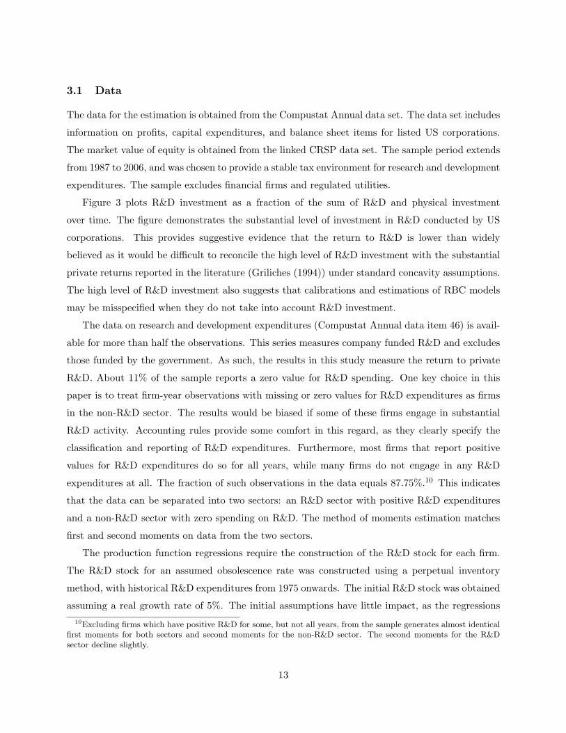
3.1 Data

The data for the estimation is obtained from the Compustat Annual data set. The data set includes

information on profits, capital expenditures, and balance sheet items for listed US corporations.

The market value of equity is obtained from the linked CRSP data set. The sample period extends

from 1987 to 2006, and was chosen to provide a stable tax environment for research and development

expenditures. The sample excludes financial firms and regulated utilities.

Figure 3 plots R&D investment as a fraction of the sum of R&D and physical investment

over time. The figure demonstrates the substantial level of investment in R&D conducted by US

corporations. This provides suggestive evidence that the return to R&D is lower than widely

believed as it would be difficult to reconcile the high level of R&D investment with the substantial

private returns reported in the literature (Griliches (1994)) under standard concavity assumptions.

The high level of R&D investment also suggests that calibrations and estimations of RBC models

may be misspecified when they do not take into account R&D investment.

The data on research and development expenditures (Compustat Annual data item 46) is avail-

able for more than half the observations. This series measures company funded R&D and excludes

those funded by the government. As such, the results in this study measure the return to private

R&D. About 11% of the sample reports a zero value for R&D spending. One key choice in this

paper is to treat firm-year observations with missing or zero values for R&D expenditures as firms

in the non-R&D sector. The results would be biased if some of these firms engage in substantial

R&D activity. Accounting rules provide some comfort in this regard, as they clearly specify the

classification and reporting of R&D expenditures. Furthermore, most firms that report positive

values for R&D expenditures do so for all years, while many firms do not engage in any R&D

expenditures at all. The fraction of such observations in the data equals 87.75%.10 This indicates

that the data can be separated into two sectors: an R&D sector with positive R&D expenditures

and a non-R&D sector with zero spending on R&D. The method of moments estimation matches

first and second moments on data from the two sectors.

The production function regressions require the construction of the R&D stock for each firm.

The R&D stock for an assumed obsolescence rate was constructed using a perpetual inventory

method, with historical R&D expenditures from 1975 onwards. The initial R&D stock was obtained

assuming a real growth rate of 5%. The initial assumptions have little impact, as the regressions

10Excluding firms which have positive R&D for some, but not all years, from the sample generates almost identicalfirst moments for both sectors and second moments for the non-R&D sector. The second moments for the R&Dsector decline slightly.

13

use observations from 1987 onwards, matching the sample selection for the structural estimation.

The log value added measure is obtained as net sales (data item 12) minus cost of goods sold (data

item 41). All variables except employment are adjusted for inflation using the GDP deflator for

non-residential investment.

Table 1 provides summary statistics for firms in the R&D and non-R&D sectors. Total assets

equals the book value of assets (data item 6). Profits equals operating income before depreciation

(data item 13) scaled by book assets. Investment is defined as capital expenditure on plant,

property, and equipment (data item 30) minus retirements of plant, property, and equipment (data

item 184). Tobin’s Q is computed as the market value of assets scaled by the book value of

assets.11 An alternative definition would be to define Q as the market value of capital scaled by

the replacement value of capital. While this definition may be preferred where measurement error

is a concern (Erickson and Whited (2000)), it also leads to large outliers, particularly in the R&D

sector, that may bias the comparison between the two sectors. The variables are Winsorized at the

99% level to eliminate outliers. The data used to compute the matched moments are adjusted for

firm and year fixed effects within the R&D and non-R&D sectors, respectively.

The moments demonstrate a sharp contrast between these two sectors, indicating fundamental

differences between firms that engage in R&D activity and those that do not. These differences

are statistically significant at the 1% level. Firms in the R&D sector have an average Tobin’s Q

value almost 50% greater than firms in the non-R&D sector (Chan, Lakonishok, and Sougiannis

(2001) find that the market value of the firm reflect R&D activity). On the other hand, these

firms exhibit much lower average earnings after accounting for their R&D expenditures. The level

of R&D spending is quite substantial when compared to total assets and larger than the rate of

investment. However, aggregate expenditures on R&D are lower than total capital expenditures

within the R&D sector, as small firms do a disproportionately larger level of R&D spending. This

is consistent with the R&D policy function given in Proposition 1 as smaller firm capture a greater

increase in firm value per unit of capital from an innovation.

3.2 Identification

The results obtained from indirect inference methods are sensitive to the choice of which specifics

moments are to be matched. In particular, it is important to select moments that are informative

11Market value of assets equals the book value of assets + market value of equity - book value of equity - deferredtaxation.

14

about the parameters of interest. Intuitively, if a given simulated moment varies strongly with a

parameter, matching this moment to the data will be informative about the underlying parameter.

The moments I match include the first moment of profits for the R&D and non-R&D sectors.

This will be informative about the parameters of the profitability process, as well as the parameters

influencing the success rate and impact of R&D spending. The second moments of profits for both

sectors help identify σ. The first and second moments of R&D spending provide information on

the R&D parameters λ, a, andγ. The first moments of Tobin’s Q for each sector help inform the

returns to scale parameter θ and the R&D parameters. The second moments of Q for both sectors

also help identify θ and the volatility of profits. The autocorrelation coefficient for profits and R&D

spending helps inform the ρ parameter. Finally, the second moment of investment identifies the

level of adjustment cost parameter b. It should be noted that each moment provides information

on almost all of the parameters.

All moments do not have the same weight in the estimation. The optimal weighting matrix

is obtained as the inverse of the covariance matrix of the chosen moments. Intuitively, the GMM

estimation works harder to match the more precisely estimated moments. Standardizing the chosen

moments by their standard errors reveals that the estimation places little weight on matching the

autocorrelation for R&D, and emphasizes the first moment of R&D, the first moment of Q for both

sectors, and the first moment of operating income for the non-R&D sector.

Some of the auxiliary parameters in the model are calibrated to simplify the estimation of the

parameters of interest. The calibrated parameters are the discount factor β, the per period fixed

cost of operations c and the depreciation rate δ. The calibrated value of β = 1/1.065 follows

Gomes (2001), Hennessy and Whited (2005), and Bloom (2008) and reflects an equity premium

of 6%. The fixed cost of operation is set at 15% of the profits prior to R&D expenditure for the

median firm in each sector.12 The depreciation rate δ = 0.079, a value which equals the mean

investment rate for all firms from the data. Setting the depreciation rate equal to the investment

rate in the data ensures that the steady state investment rate in the simulated data, which equals

the depreciation rate, matches the actual data. One could easily match the mean investment rates

for the two sectors separately by specifying different depreciation rates. The fraction of firms in

the R&D sector equals 0.48, the fraction of observations with positive R&D values in the data set.

The µ parameter is not identified with the chosen moments as it functions as a scaling parameter.

As such, fix µ = −0.3 for both sectors. The chosen moments do not include the relative firm size

12Eberly, Rebelo, and Vincent (2008) estimates fixed costs to be 22% of revenue net of variable costs includingR&D expenditures.

15

between R&D and non-R&D firms. This could be matched by allowing µ to vary across the two

sectors.

3.3 Estimating the return using production functions

This section details the observation that the production function approach pioneered by Griliches

(1979) suffers from an indeterminacy flaw when applied to estimating the return to R&D. This

approach specifies value-added by the firm as a multiplicative function of factor inputs, including

the R&D stock:

Yi,t = atKαi,tL

βi,tS

νi,t. (13)

A linear regression of log value-added on log inputs yields the elasticity of value-added with respect

to the R&D stock ν. The construction of the R&D stock Si,t follows a perpetual inventory method

using data on R&D expenditures applied to equation (4). The obsolescence rate of R&D investment

necessary for the construction of the R&D stock is typically assumed to be 15%, following Griliches

and Mairesse (1984), or sometimes assumed to be 0. One common finding in this literature is that

the estimated elasticity ν does not vary with the assumed obsolescence rate γ.

The return to R&D in this framework equals the marginal product of R&D on value-added and

is given by:∂Yi,t

∂Si,t= ν

Yi,t

Si,t.

The calculated R&D stocks vary with the assumed obsolescence rate γ. This can be most easily

seen by considering a firm that invests a fixed amount R in R&D. The R&D stock of this firm is

given by S = Rγ. However, while the calculated R&D stocks vary with γ, the ν estimates does not

(Hall and Mairesse (1995)). This implies that the estimated rates of return obtained using this

framework are sensitive to the assumed obsolescence rate γ. The intuition for this result is that

higher obsolescence rates lead to a lower R&D stock, resulting in a higher marginal impact of R&D

on value added, as the elasticity parameter remains mostly unchanged.

Table 2 presents the results of the above regression for different assumptions on γ using the

Compustat data set. Note that even though the notation is identical, γ may not be comparable

across the two approaches as the R&D stock concept in the production function regression differs

from the R&D stock concept in the structural model. The sample ranges from 1987 to 2006, and all

variables except employment are adjusted for inflation using the GDP deflator for non-residential

investment. The pooled regression includes year and industry dummies, and the standard errors

16

are robust to clustering at the firm level. The assumed obsolescence rates range from 0 to 0.25.

The regressions reveal that the estimated elasticity of value-added with respect to R&D varies

little with the obsolescence rate γ, as commonly found in the literature. The point estimate implies

an economically and statistically significant contribution of R&D to value-added by firms. The

adjusted R-square values indicate that the model fit does not vary much with γ.

The table reports the sample median steady state return for a hypothetical firm with a constant

R&D policy and the sample median return using the computed R&D stocks. Both return estimates

vary sharply with the obsolescence rate γ. Using the standard assumption of γ = 0.15 leads to

an estimated median return of 45.2%, similar to the high rates of return reported in the literature

(see Griliches (1986) and Hall and Mairesse (1995)). However, changing the assumed value of γ to

0 yields a much lower return (12.6%), and assuming γ = 0.25 yields an even higher return. The

steady state returns with a fixed R&D policy exhibit similar variation. Thus, the return estimates

obtained from production function regressions vary sharply with the assumed obsolescence rates, a

difficulty compounded by the lack of evidence on the appropriate value for γ.

4 Results from structural estimation

4.1 Baseline model

The estimation begins with the baseline model, which identifies the impact of R&D on profits, the

success rate from R&D, and the rate of depreciation for R&D stocks. Table 3 presents the results

of estimating the model by indirect inference. Panel A reports the matched moments for the data

and simulations, respectively. Panel B reports the estimated parameter values. Panel C reports

some statistics of economic interest from the simulated data set.

The low value for the J -statistic demonstrates that the model matches the chosen moments

well. Examination of the matched moments indicates that the model succeeds in matching the first

and second moments of R&D to assets. The model also matches the first moment of Tobin’s Q for

both sectors, and matches the second moment of Tobin’s Q for the non-R&D sector. While the

measure of Tobin’s Q in the simulated data incorporates the R&D stock it also reflects differences

in growth options due to potential innovations. The model fares less well at matching the first and

second moments of income for both sectors. The estimation yields a ρ value that is much higher

than regression estimates, thereby resulting in higher autocorrelations for both profits and R&D

17

expenditures.

The model has trouble generating the high level of Tobin’s Q given the observed levels of profits.

A related difficulty arises from matching the variation in Tobin’s Q given the variation in profits. A

high autocorrelation value helps with both of these challenges. For a given distribution of profits,

an increase in persistence will increase Tobin’s Q for high profitability firms and lower it for low

profitability firms. This impact will be greater for high Q firms, resulting in higher first and second

moments for Tobin’s Q. A high autocorrelation value also increases R&D investment by extending

the benefit of an innovation further into the future.

The results indicate that firms in the R&D sector generate an economically and statistically

significant increase in profitability from a successful innovation. The point estimate for λ of 0.123

implies that a successful innovation increases the profitability of the firm by 13.1%. Ignoring any

changes in the capital stock, this is equivalent in present value terms to a 9.0% permanent increase in

profitability. In the steady state, 50.7% of firms in the R&D sector innovate each period. However,

there is sharp cross-sectional variation in the probability of innovation, reflecting the sensitivity of

the R&D policy function on the current profitability and size of the firm.

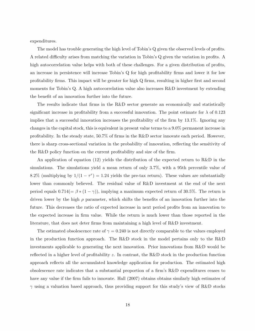
An application of equation (12) yields the distribution of the expected return to R&D in the

simulations. The simulations yield a mean return of only 3.7%, with a 95th percentile value of

8.2% (multiplying by 1/(1 − τ r) = 1.24 yields the pre-tax return). These values are substantially

lower than commonly believed. The residual value of R&D investment at the end of the next

period equals 0.714(= β ∗ (1 − γ)), implying a maximum expected return of 30.5%. The return is

driven lower by the high ρ parameter, which shifts the benefits of an innovation further into the

future. This decreases the ratio of expected increase in next period profits from an innovation to

the expected increase in firm value. While the return is much lower than those reported in the

literature, that does not deter firms from maintaining a high level of R&D investment.

The estimated obsolescence rate of γ = 0.240 is not directly comparable to the values employed

in the production function approach. The R&D stock in the model pertains only to the R&D

investments applicable to generating the next innovation. Prior innovations from R&D would be

reflected in a higher level of profitability z. In contrast, the R&D stock in the production function

approach reflects all the accumulated knowledge application for production. The estimated high

obsolescence rate indicates that a substantial proportion of a firm’s R&D expenditures ceases to

have any value if the firm fails to innovate. Hall (2007) obtains obtains similarly high estimates of

γ using a valuation based approach, thus providing support for this study’s view of R&D stocks

18

as measuring the stock of experiments towards the next innovation. It is less plausible to view the

stock of ideas applicable for production becoming obsolete at these rates. The γ estimate implies a

half-life of R&D expenditures of 2.53 years, indicating a moderate lifespan for R&D projects. The

point estimate for the adjustment cost parameter b matches those found by Whited (1992), Cooper

and Haltiwanger (2006), and Eberly, Rebelo, and Vincent (2008).

The steady state mean expected increase in firm value equals 21.3%, with a high degree of cross-

sectional variation. A high impact of innovation on firm value induces firms to incur the high level

of R&D expenditures observed in the data and the simulations despite the low return estimates.

While the appropriate sample counterpart is unclear, the estimate is consistent with anecdotal

evidence of sudden jumps in firm value upon the release of news about potential innovations.

The estimation yields a value of the aggregate R&D stock equal to 17.9% of the value of all

capital.13 In comparison, the aggregate value of R&D investment to all investment in the sample

period equals 24.6%. This indicates that a substantial portion of the aggregate capital stock consists

of R&D stocks. As R&D stocks comprise a large fraction of all intangible capital, these findings

support the argument of Hall (2001) that intangible capital accumulation forms an important

component of US investment.

4.2 Estimates with a lower discount rate

The estimates of the baseline model indicate that the model has difficulty reconciling the profit and

valuation levels. This has the effect of yielding a very high autocorrelation parameter, as the model

strives to reconcile a low level of profits with the observed valuations. One solution to this difficulty

is to assume a lower discount rate. The value of β = 1/1.065 used in the baseline estimation is

calibrated assuming a 6% equity premium. Recent evidence indicates that the equity premium

may have been sharply lower for this sample period, motivating a higher value for β. This section

reports the results using a discount rate of β = 1/1.045 to estimate the model.14

Table 4 presents the results using the lower discount rate. Panel A reports the matched moments

for the data and simulations, respectively. Panel B reports the estimated parameter values. Panel

13The R&D Satellite accounts recently constructed by the BEA measures the book value of R&D stocks to be 7.3%of the sum of R&D and physical capital as of 2003.

14Fama and French (2002) find an equity premium in the range of 2.55% to 4.32% using dividend and earningsgrowth rates. Claus and Thomas (2001) find an equity premium in the range of 3% from 1985 to 1998 using analystsforecasts. Jagannathan, McGrattan, and Scherbina (2001) find an equity premium of almost zero for 1982 to 1999using data on bond yields and dividend yields. Cogley and Sargent (2008) argue that the declining equity premiumarises due to a pessimistic prior following the Great Depression. The implied equity premium of 4% is at the highend of these estimates.

19

C reports some statistics of economic interest from the simulated data set.

The value of the J -statistic is lower than that for the baseline model. As suggested above, this

model has better success reconciling the moments on profits with the valuation moments. The

lower discount rate also leads to a lower autocorrelation parameter. The estimates continue to

have difficulty with the second moment of Tobin’s Q, as the model does not generate as many

observations with high Tobin’s Q as found in the data. Overall, the lower discount rate improves

the performance of the model.

The point estimate for λ implies a 18.9% increase in profitability from a successful innovation.

This is larger than the corresponding value obtained in the baseline estimation because the lower

value of ρ requires an innovation to have a greater initial impact on profits, as the benefit dissipates

faster. In present value terms, the estimate corresponds to a 4.63% permanent increase in profitabil-

ity, lower than the comparable estimate for the baseline model. The smaller permanent increase in

profits generates a similar level of R&D expenditures, as the firms discount future dividends less

than before. The steady state rate of innovation is lower, with a mean probability of success of

0.450.15 This is partly due to the higher obsolescence rate γ, which implies a lower steady state

R&D stock than in the baseline model.

The steady state mean return to R&D expenditures equals 5.5%, higher than the estimated value

from the baseline model. Nonetheless, this estimate is much lower than the values reported in the

literature. Intuitively, the lower estimate for ρ implies that more of the benefit of an innovation

is realized in the next period, thereby increasing the ratio of expected increase in profits from an

innovation to the expected increase in firm value. The higher estimate of γ decreases the residual

value of R&D expenditures, also resulting in a higher return. However, the higher return does not

translate to a higher level of R&D expenditures.

The difference in expected firm value from innovating versus not-innovating has a direct impact

on R&D policy in the model. The mean expected increase in firm value of 14.1% is lower than the

corresponding value in the baseline model. There is also much less cross-sectional variation in the

increase in firm value. The higher impact of a successful innovation on profits does not translate

to firm values, as the benefit dissipates faster.

15The 5th percentile of the probability of success equals 0, as 8.1% of firms in the steady state have an R&D stockof 0.

20

4.3 Estimates using only R&D sector data

The results presented in the baseline model assume that the non-R&D related parameters are

identical across both sectors and use non-R&D sector data to help estimate these parameters.

However, these parameters may vary across the two sectors. This section presents the results of

estimating the model using data only on R&D sector firms. This leads to a decrease in the number

of matched moments and provides a robustness check to differences in model parameters across the

two sectors.

Table 5 presents the results of estimating the model using indirect inference with data on R&D

sector firms only. Panel A reports the matched moments for the data and simulations, respectively.

Panel B reports the estimated parameter values. Panel C reports some statistics of economic interest

from the simulated data set. The calibrated value of δ = 6.3%, the mean capital investment rate

for R&D sector firms. The discount rate β = 1/1.065, as in the baseline model.

The matched moments exhibit a similar pattern to that observed in Table 3. The model matches

the first and second moments of R&D and has difficulty reconciling the level of profitability with

the level of Tobin’s Q. The model also implies a higher autocorrelation level for profits and R&D

than found in the data. The J-statistic increases and its p-value decreases, as the number of data

points and the degrees of freedom decrease. However, the data does not reject the model.

The point estimates imply a higher impact of an innovation on profits and a higher obsolescence

rate for R&D expenditures. The lower point estimate for θ suggests that mark-ups may be slightly

higher in the R&D sector. Somewhat surprisingly, the measures of economic interest are quite

similar to those obtained using data on both sectors. The return to R&D is, as before, much lower

than that reported in the literature. The probability of an innovation exhibits sharp cross-sectional

variation and is slightly lower than the baseline model estimate.

The above estimates indicate that firms capture an economically and statistically significant

increase in profits from innovation. They also face significant uncertainty regarding the outcome

of their R&D expenditures. This uncertainty does not, however, deter firms from undertaking the

substantial level of R&D expenditures observed in the data.

5 Policy experiments

This section presents the results of counterfactual experiments on the following: a subsidy on R&D

spending and an increase in the impact of a successful innovation on profits. The policy experiments

21

reflect the model and are partial equilibrium in nature. They do not take into account possible

responses by consumers or changes in government spending arising from these exogenous changes.

As such, substantial care needs to be taken in using these experiments to argue for policy changes.

The analysis provides a method to quantify the impact of changes in key parameters on the level

of R&D spending, profits, firm value, and the rate of innovation within the context of the model.

5.1 A subsidy to R&D spending

There exists an active policy debate about using the tax code to subsidize R&D investment. The

research and experimentation tax credit uses a complex formula based on growth rates in these

expenditures, which comprise only a subset of total R&D expenditures. The estimation presented

in the previous section accounts for the tax credit through the calibration of the gross tax rate

on operating income, τ r. The tax credit amounted to about 2.5% of all spending on R&D by

firms from 1990 to 2001 (Moris (2005)). Currently, the tax credit is not permanent and requires

Congressional authorization every few years. This counterfactual experiment studies the impact of

a further 5% R&D tax credit within the context of the model (see Bloom, Griffith, and van Reenen

(2002) for a cross-country study on the impact of tax subsidies on innovation). Table 6 reports the

moments of interest using the actual estimates and with a 5% subsidy on R&D expenditures. Panel

A reports the values for the baseline model, Panel B reports the values with the lower discount

rate parameter, and Panel C reports the results with the R&D sector only estimates. While the

analysis does not impose any other taxes to offset the drop in tax revenue, it can provide a basis

for a cost-benefit analysis of R&D tax credits.

The subsidy for R&D expenditures leads to higher spending and a greater level of innovation

under all models. The tax subsidy increases the rate of innovation by 4.4, 3.6, and 4.4 percentage

points for the models estimated in Sections 4.1, 4.2, and 4.3, respectively. This is driven by an

approximately 1% increase in the rate of R&D expenditures in response to the additional tax

credit. The findings imply a mean increase in R&D expenditures of 1.72 to 2.15 dollars for a dollar

increase in the R&D tax credit. This is higher than the 1 to 1 impact of R&D tax credits on R&D

expenditures estimated by Hall and van Reenen (2000). The similar impact of the tax subsidy for

all models contrasts with the different rates of return. This provides further evidence that using

the return to R&D for policy prescriptions leads to erroneous conclusions in this setting.

22

5.2 An increase in the impact of a successful innovation

An increase in the impact of a successful innovation provides a method to incorporate changes in

patent policy that favor innovators into the model. Eaton and Kortum (1999) directly estimate

a model of international research and patenting and find a strong effect of strengthening patent

rights on productivity growth. While such an analysis does not shed much light on the optimal

level of patent protection, it can help quantify the impact of a change in patent policy on R&D

expenditures and the rate of innovation. Gilbert and Shapiro (1990) argue for viewing patent policy

in terms of the degree of profits accruing to the innovator. In the context of this study, increased

patent protection can be viewed as an exogenous increase in λ. Table 7 reports the moments of

interest using the actual estimates and the new values obtained with a 5% increase in λ. Panel A

reports the values for the baseline model, Panel B reports the values with the lower discount rate

parameter, and Panel C reports the results with the R&D sector only estimates.

The increase in the impact of a successful innovation on profits leads to higher investment

in R&D for all models. The rate of innovation increases by 3.7, 3.2, and 3.6 percentage points,

respectively. The increase in λ has a similar impact on the rate of innovation as the R&D tax

subsidy. However, this experiment has a larger impact on valuation compared to the tax subsidy.

The tax subsidy benefits all R&D firms, while the increase in λ benefits only firms that innovate.

As firms with higher valuations invest more in R&D and are more likely to innovate, the change in

λ has a bigger impact on these firms, as reflected in the larger increase in the mean value of Tobin’s

Q.

6 Conclusion

An empirical analysis demonstrates that the high returns to R&D found in much of the literature

are sensitive to assumptions of the obsolescence rate. This study estimates the return to R&D by

simultaneously estimating all the key structural parameters of a dynamic model. The underlying

model differs from that used in the production based approach as it incorporates uncertainty in

the outcome of R&D projects, an arguably key economic feature of R&D investment. Further, the

R&D stock in the model measures investment made towards generating the next innovation instead

of the knowledge stock applicable for production. The identified variables of interest include the

impact of an innovation on profits, the rate of innovation, the return to R&D, and the expected

increase in firm value from an innovation.

23

The estimates reveal an economically and statistically significant impact of an innovation on

profits. In present value terms, an innovation leads to an increase in profitability of 4.6-9.0%. This

translates to an expected increase in firm value from innovating of 14.1-21.3%. The estimated

rates of innovation suggest a significant probability of failure for R&D projects, highlighting the

importance of uncertainty in estimating the return to R&D. The estimated returns to R&D are

much lower than those found in the literature. However, this does not deter firms from maintaining

a high level of R&D investment.

Counterfactual experiments examine the impact of a subsidy to R&D expenditures and an

increase in profits from a successful innovation. A tax subsidy yields a clear increase in the rate

of innovation even though the estimates imply a low return. These findings suggests that, as it

focuses only on the short-term impact, the return to R&D would not be an appropriate tool for

R&D policy analysis.

The analysis in this study employs a partial equilibrium approach that does not incorporate

economic growth. Combining the findings of this study with endogenous growth models, such as

that by Klette and Kortum (2004), may provide a rich framework for further research and policy

analysis.

24

Appendix

A Proofs

Proposition 1 The optimal R&D stock of the firm when S′

i > 0 is given by

S′

i

Ki=

1

a

[

log(a) − log ((1 − τ r)(1 − β(1 − γ))) + log

(

β(Ez[G(K ′

i, z′

i)|ji = 1] − Ez[G(K ′

i, z′

i)|ji = 0])

Ki

)]

.

Proof. The first order condition for the optimal R&D stock yields:

− (1 − τ r) + (1 − τ r)β(1 − γ) + β∂Ez[G(K ′

i, z′

i)]

∂S′

i

= 0. (A.1)

The impact of R&D spending on the expected value of the firm in the next period can be clarified

by an application of the law of iterated expectations,

Ez[G(K ′

i, z′

i)] = Ez[G(K ′

i, z′

i)|ji = 1]p(ji = 1) + Ez[G(K ′

i, z′

i)|ji = 0]p(ji = 0).

This result arises due to the independence between the draws of ji and εi. Substituting the expres-

sion for p(ji) given in (5) one obtains:

Ez[G(K ′

i, z′

i)] = Ez[G(K ′

i, z′

i)|ji = 1](1 − exp(−aS′

i

Ki)) + Ez[G(K ′

i, z′

i)|ji = 0] exp(−aS′

i

Ki). (A.2)

The derivative of the above expression with respect to S′

i yields:

∂Ez[G(K ′

i, z′

i)]

∂S′

i

=a

Kiexp(−a

S′

i

Ki)(

Ez[G(K ′

i, z′

i)|ji = 1] − Ez[G(K ′

i, z′

i)|ji = 0])

.

Substituting the above expression into the first order condition given in (A.1) yields the optimal

policy function for the firm’s R&D stock,

(1 − τ r)(1 − β(1 − γ)) = βa

Kiexp(−a

S′

i

Ki)(

Ez[G(K ′

i, z′

i)|ji = 1] − Ez[G(K ′

i, z′

i)|ji = 0])

(A.3)

⇒ S′

i

Ki=

1

a

[

log(a) − log ((1 − τ r)(1 − β(1 − γ))) + log

(

β(Ez[G(K ′

i, z′

i)|ji = 1] − Ez[G(K ′

i, z′

i)|ji = 0])

Ki

)]

.

25

Some algebra reveals that the second order condition with respect to S′

i is negative, ensuring that

the F.O.C.s yield the optimal policy in the interior region.

B Expected return to R&D

The after-tax expected return to R&D expenditures is given by:

∂

∂Si′Ez

[

Π(K ′

i, z′

i)(1 − τ r)]

=∂

∂Si′Ez

[

z′i(K′

i)θ(1 − τ r)

]

. (B.1)

The conditional expectation of z′i can be written as,

Ez[z′

i] = Ez[z′

i|ji = 1]p(ji = 1) + Ez[z′

i|ji = 0]p(ji = 0). (B.2)

Using the transition equation for z′i in (6) and the log-normality assumption, the conditional ex-

pectations can be written as

Ez

[

z′i|ji = 1]

= exp(

µ + λ + ρ log(zi) + σ2/2)

= zρi exp

(

µ + σ2/2 + λ)

.

Ez

[

z′i|ji = 0]

= zρi exp

(

µ + σ2/2)

.

The partial derivative of the probability of an innovation equals:

∂

∂Si′p(ji = 1) =

a

Kiexp(−a

S′

i

Ki). (B.3)

The above expressions yield the following:

∂

∂Si′Ez

[

Π(K ′

i, z′

i)]

= (K ′

i)θ

[

zρi exp

(

µ + σ2/2 + λ) a

Kiexp(−a

S′

i

Ki) − zρ

i exp(

µ + σ2/2) a

Kiexp(−a

S′

i

Ki)

]

= (K ′

i)θ a

Kiexp(−a

S′

i

Ki)zρ

i exp(

µ + σ2/2)

[exp(λ) − 1].

26

Substituting the expression for aKi

exp(−aS′

i

Ki) given in (A.3) and collecting terms yields the following

expression for the return to R&D.:

∂

∂Si′Ez

[

Π(K ′

i, z′

i)(1 − τ r)]

=

(

(K ′

i)θzρ

i exp(

µ + σ2/2)

[exp(λ) − 1]

Ez[G(K ′

i, z′

i)|ji = 1] − Ez[G(K ′

i, z′

i)|ji = 0]

)

(1 − β(1 − γ))

β.

C Simulated method of moments

The indirect inference method of Gourieroux, Monfort, and Renault (1993) obtains parameter

estimates by matching a set of selected moments from the data to those obtained by simulation.

Denote the structural parameters by Ψ∗. The matched moments can be written as a solution to

a minimization problem Q(Y, M), where Y denotes the data and M the moments to be matched.

The data moments are then given by

M = arg minM

Q(YN , M), (C.1)

where YN denotes a data matrix with N observations. The corresponding moments for the simulated

data set with parameter vector Ψ and n = N × S observations are given by

m(Ψ) = arg minM

Q(Ym, M). (C.2)

The study picks S = 8, which is within the recommended range.

The structural parameters are then obtained by minimizing a quadratic form of the distance

between the data and simulated moments.

Ψ = arg minΨ

[

M − m(Ψ)]

′

W[

M − m(Ψ)]

, (C.3)

where W denotes a positive definite weighting matrix. The optimal weighting matrix is given by

W =[

Nvar(M)]

−1. (C.4)

The above covariance matrix is calculated with the actual data set using the influence function

method of Erickson and Whited (2000). The estimator is asymptotically normal for fixed S with

27

covariance matrix given by

√N(Ψ − Ψ∗) ∼ N(0, Φ) (C.5)

Φ = (1 +1

S)

[

∂2Q

∂Ψ∂M ′

(

∂Q

∂M

∂Q

∂M

′)

−1∂2Q

∂M∂Ψ′

]

−1

.

While ∂Q∂M

can be evaluated analytically, numerical methods are required to obtain ∂2Q∂Ψ∂M

. Both

partial derivatives are obtained using simulated data evaluated at the data moments.

The indirect inference method also yields a GMM-style test of the over-identifying restrictions.

The J-statistic adjusted for the simulation size converges in distribution to a χ2 distribution, with

degrees of freedom equal to the number of moments minus the number of parameters:

J =NS

1 + S

[

M − m(Ψ)]

′

W[

M − m(Ψ)]

. (C.6)

D Numerical Solution

The simulations require numerical solution of the value function for firms in the R&D and non-

R&D sectors. The capital grid has 61 points and the profits grid has 10 points. The capital

grid is centered around an approximation of the median size of the firm given the parameters.

Simulations which result in steady state firm sizes near the boundaries of the grid are discarded

in the estimation. The profit grid is formed using the quadrature method of Tauchen and Hussey

(1991), with a mean value obtained by guessing the success rate. The endogenous jumps in z from

an innovation are handled by interpolating firm value over two more grids constructed using the

transition equation for profitability conditional on whether the firm innovates. The expected value

of the firm is obtained using the law of iterated expectations.

The simulated sample is generated using the value and policy functions for the R&D and non-

R&D sectors. The law of motion for profitability is generated directly using the transition equations

(6) and (2). The firm’s decisions are obtained using linear interpolation of the policy functions. The

simulations maintain the same fraction of firms in the R&D sector as in the data. The simulation

is run for 100 years, with the initial 50 discarded as a burn-in sample. This yields the value of

the quadratic form of the difference in the data moments and simulated moments. The program

searches for the parameters that minimize this distance using the simulated annealing algorithm.

Each estimation involved evaluating more than 100,000 candidate parameter sets.

28

References

Abel, Andrew, and Janice C. Eberly, 1994, A unified model of investment under uncertainty,

American Economic Review 84, 1369–1384.

Aghion, Philippe, Nick Bloom, Richard Blundell, Rachel Griffith, and Peter Howitt, 2005, Compe-

tition and innovation: An inverted-U relationship, Quarterly Journal of Economics 120, 701–728.

Aghion, Philippe, and Peter Howitt, 1992, A model of growth through creative destruction, Econo-

metrica 60, 323–351.

Barlevy, Gadi, 2007, On the cyclicality of research and development, American Economic Review

97, 1131–1164.

Bertsekas, Dimitri P., 2000, Dynamic Programming and Optimal Control vol. 1. (Athena Scientific

Belmont, MA).

Bloom, Nick, 2008, The impact of uncertainty shocks, Forthcoming, Econometrica.

Bloom, Nick, Rachel Griffith, and John Van Reenen, 2002, Do R&D tax credits work? Evidence

from a panel of countries 1979-1997, Journal of Public Economics 85, 1–31.

Bloom, Nick, Mark Schankerman, and John Van Reenen, 2007, Identifying technology spillovers

and product market rivalry, NBER working paper 13060.

Boldrin, Michele, and David K. Levine, 2008, Perfectly competitive innovation, Journal of Monetary

Economics 55, 435–453.

Brown, James R., Steven M. Fazzari, and Bruce C. Petersen, 2008, Financing innovation and

growth: Cash flow, external equity and the 1990s R&D boom, Forthcoming, Journal of Finance.

Chan, Louis K. C., Josef Lakonishok, and Theodore Sougiannis, 2001, The stock market valuation

of research and development expenditures, Journal of Finance 56, 24312456.

Claus, James, and Jacob Thomas, 2001, Equity premia as low as three percent? Evidence from

analysts’ earnings forecasts for domestic and international stock markets, Journal of Finance 56,

1629–1666.

Cogley, Timothy, and Thomas J. Sargent, 2008, The market price of risk and the equity premium:

A legacy of the Great Depression?, Journal of Monetary Economics 55, 454–476.

29

Comin, Diego, and Mark Gertler, 2006, Medium-term business cycles, Americal Economic Review

96, 523–551.

Cooper, Russell W., and Joao Ejarque, 2003, Financial frictions and investment: Requiem in Q,

Review of Economic Dynamics 6, 710–728.

Cooper, Russell W., and John Haltiwanger, 2006, On the nature of capital adjustment costs, Review

of Economic Studies 73, 611–633.

Eaton, Jonathan, and Samuel Kortum, 1999, International technology diffusion: Theory and mea-

surement, International Economic Review 40, 537–570.

Eberly, Janice, Sergio Rebelo, and Nicolas Vincent, 2008, Investment and value: A neoclassical

benchmark, NBER Working Paper 13866.

Erickson, Timothy, and Toni M. Whited, 2000, Measurement error and the relationship between

investment and q, Journal of Political Economy 108, 1027–1057.

Fama, Eugene F., and Kenneth R. French, 2002, The equity premium, Journal of Finance 57,

637–659.

Gilbert, Richard, and Carl Shapiro, 1990, Optimal patent length and breath, RAND Journal of

Economics 26, 106–112.

Gomes, Joao F., 2001, Financing investment, American Economic Review 90, 1263–1285.

Gourieroux, Christian, Alain Monfort, and E. Renault, 1993, Indirect inference, Journal of Applied

Econometrics 8, S85–S118.

Greenwood, Jeremy, and Boyan Jovanovic, 1999, The information-technology revolution and the

stock market, American Economic Association (Papers and Proceedings) 89, 116–122.

Griliches, Zvi, 1979, Issues in assessing the contribution of research and development to productivity

growth, Bell Journal of Economics 10, 92–116.

Griliches, Zvi, 1986, Productivity, R&D, and basic research at the firm level in the 1970’s, American

Economic Review 76, 141–154.

Griliches, Zvi, 1994, Productivity, R&D, and the data constraint, American Economic Review 84,

1–23.

30

Griliches, Zvi, and Jacques Mairesse, 1984, Productivity and R&D at the firm level, in Zvi Griliches,

eds.: R & D, Patents, and Productivity (University of Chicago Press, Chicago, IL ).

Grossman, Gene M., and Elhanan Helpman, 1991, Innovation and Growth in the Global Economy.

(MIT Press Boston, MA).

Hall, Bronwyn H., 2007, Measuring the returns to R&D: The depreciation problem, NBER working

paper 13473.

Hall, Bronwyn H., and Jacques Mairesse, 1995, Exploring the relationship between R&D and

productivity in French manufacturing firms, Journal of Econometrics 65, 263–293.

Hall, Bronwyn H., and John Van Reenen, 2000, How effective are fiscal incentives for R&D? A

review of the evidence, Research Policy 29, 449–469.

Hall, Robert E., 2001, The stock market and capital accumulation, American Economic Review

91, 1185–1202.

Hennessy, Christopher A., and Toni M. Whited, 2005, Debt dynamics, Journal of Finance 60,

1129–1165.

Hennessy, Christopher A., and Toni M. Whited, 2007, How costly is external financing? Evidence

from a structural estimation, Journal of Finance 62, 1705–1745.

Hobijn, Bart, and Boyan Jovanovic, 2001, The information-technology revolution and the stock

market: Evidence, American Economic Review 91, 1203–1220.

Jagannathan, Ravi, Ellen R. McGrattan, and Anna Scherbina, 2001, The declining U.S. equity

premium, Federal Reserve Bank of Minneapolis Quarterly Review 24, 3–19.

Jones, Charles I., 1995a, R&D-based models of economics growth, Journal of Political Economy

103, 759–784.

Jones, Charles I., 1995b, Time series tests of endogenous growth models, Quarterly Journal of

Economics 110, 495–525.

Jones, Charles I., and John C. Williams, 1998, Measuring the social return to R&D, Quarterly

Journal of Economics 113, 1119–1135.

31

Klette, Tor Jacob, and Samuel Kortum, 2004, Innovating firms and aggregate innovation, Journal

of Political Economy 112, 986–1018.

Kortum, Samuel, 1997, Research, patenting and technological change, Econometrica 65, 1389–1419.

Li, Dongmei, 2007, Financial constraints, R&D investment, and stock returns: Theory and evi-

dence, Working paper, University of California, San Diego.

Moris, Francisco, 2005, The U.S. research and experimentation tax credit in the 1990s, National

Science Foundation, InfoBrief NSF05-316, Arlington, VA.

Romer, Paul M., 1990, Endogenous technological change, Journal of Political Economy 98, S71–

S102.

Segerstrom, Paul S., 1998, Engogenous growth without scale effects, American Economic Review

88, 1290–1310.

Stokey, Nancy L., and Robert E. Lucas, Jr., 1989, Recursive Methods in Economic Dynamics.

(Harvard University Press, Cambridge, MA).

Tauchen, George, and Robert Hussey, 1991, Quadrature-based methods for obtaining approximate

solutions to nonlinear asset pricing models, Econometrica 59, 371–396.

Whited, Toni M., 1992, Debt, liquidity constraints, and corporate investment: Evidence from panel

data, Journal of Finance 47, 1425–1460.

Young, Alywn, 1998, Growth without scale effects, Journal of Political Economy 106, 41–63.

32

Table 1: Summary statistics

The table reports summary statistics for firms classified by their R&D investment into the R&D andnon-R&D sectors. The data are at an annual frequency. The source data are from the CompustatIndustrial files from 1987 to 2006. All variables are scaled by the book value of assets of thefirm and Winsorized at the 1% level. Tobin’s Q is defined as the market value of assets scaledby the book value of assets. Profits equals operating income before depreciation scaled by bookassets. R&D expenditure is obtained from Compustat data item 46 and treated as an expensein calculating profits. Investment equals capital expenditures on plant, property, and equipmentnet of retirements. The variables are adjusted for firm and year fixed effects within the R&D andnon-R&D sectors.

R&D sector Non-R&D sectorVariable Mean Std. Dev. Mean Std. Dev.

Log assets 5.034 2.131 5.193 1.860Tobin’s Q 2.174 1.224 1.528 0.680Profits 0.072 0.146 0.144 0.100R&D to assets 0.112 0.082Investment to assets 0.063 0.062 0.094 0.089Number of observations 35409 38207

33

Table 2: Production function regressions

The table reports the results of a pooled regression of the log of value-added on logs of labor,capital, and the stock of R&D. The regressors include year and industry dummies. The pointestimates yield the estimated elasticities of value added with respect to the inputs. The columnsvary the assumed obsolescence rate in the construction of the R&D stock. The standard errorsare heteroskedasticity robust and adjust for clustering at the firm level. The R&D stock variableis constructed using a perpetual inventory method. The data are from the Compustat annual filefrom 1987 to 2006. All variables, except labor, are adjusted for inflation using the GDP deflatorfor business investment. The steady state return to R&D, which equals ν Y

Rγ, is derived using the

estimated R&D elasticity ν, the assumed obsolescence rate γ, and the sample median value of theratio of value added to R&D expenditures. The sample median of Y

Requals 8.63. The estimated

return to R&D, which equals ν YS

, uses the estimated elasticity ν and the sample median of valueadded scaled by the R&D stock, which varies with the assumed obsolescence rate γ.

Obsolescence rateRegressor γ = 0 γ = 0.05 γ = 0.10 γ = 0.15 γ = 0.25

Labor 0.656 0.650 0.649 0.648 0.648(0.016) (0.016) (0.016) (0.016) (0.016)

Capital stock 0.181 0.169 0.162 0.157 0.152(0.012) (0.012) (0.012) (0.012) (0.012)

R&d stock 0.197 0.216 0.225 0.229 0.234(0.008) (0.009) (0.008) (0.008) (0.008)

Number of Observations 39582 39582 39582 39582 39582Adjusted R-squared 0.892 0.894 0.895 0.896 0.896

Steady state return (= ν YR

γ) - 9.3% 19.4% 29.7% 50.4%

Estimated return (= ν YS

) 12.6% 24.1% 34.8% 45.2% 65.0%

34

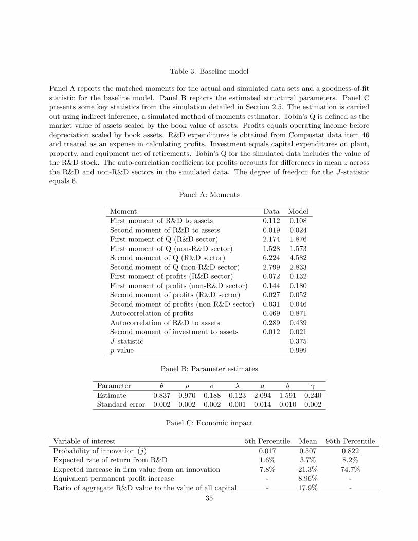
Table 3: Baseline model

Panel A reports the matched moments for the actual and simulated data sets and a goodness-of-fitstatistic for the baseline model. Panel B reports the estimated structural parameters. Panel Cpresents some key statistics from the simulation detailed in Section 2.5. The estimation is carriedout using indirect inference, a simulated method of moments estimator. Tobin’s Q is defined as themarket value of assets scaled by the book value of assets. Profits equals operating income beforedepreciation scaled by book assets. R&D expenditures is obtained from Compustat data item 46and treated as an expense in calculating profits. Investment equals capital expenditures on plant,property, and equipment net of retirements. Tobin’s Q for the simulated data includes the value ofthe R&D stock. The auto-correlation coefficient for profits accounts for differences in mean z acrossthe R&D and non-R&D sectors in the simulated data. The degree of freedom for the J-statisticequals 6.

Panel A: Moments

Moment Data Model

First moment of R&D to assets 0.112 0.108Second moment of R&D to assets 0.019 0.024First moment of Q (R&D sector) 2.174 1.876First moment of Q (non-R&D sector) 1.528 1.573Second moment of Q (R&D sector) 6.224 4.582Second moment of Q (non-R&D sector) 2.799 2.833First moment of profits (R&D sector) 0.072 0.132First moment of profits (non-R&D sector) 0.144 0.180Second moment of profits (R&D sector) 0.027 0.052Second moment of profits (non-R&D sector) 0.031 0.046Autocorrelation of profits 0.469 0.871Autocorrelation of R&D to assets 0.289 0.439Second moment of investment to assets 0.012 0.021J -statistic 0.375p-value 0.999

Panel B: Parameter estimates

Parameter θ ρ σ λ a b γ

Estimate 0.837 0.970 0.188 0.123 2.094 1.591 0.240Standard error 0.002 0.002 0.002 0.001 0.014 0.010 0.002

Panel C: Economic impact

Variable of interest 5th Percentile Mean 95th Percentile

Probability of innovation (j) 0.017 0.507 0.822Expected rate of return from R&D 1.6% 3.7% 8.2%Expected increase in firm value from an innovation 7.8% 21.3% 74.7%Equivalent permanent profit increase - 8.96% -Ratio of aggregate R&D value to the value of all capital - 17.9% -

35

Table 4: Model with lower discount rate

Panel A reports the matched moments for the actual and simulated data sets and a goodness-of-fit statistic for the model with a lower discount rate. Panel B reports the estimated structuralparameters. Panel C presents some key statistics from the simulation detailed in Section 2.5.The estimation is carried out using indirect inference, a simulated method of moments estimator.Tobin’s Q is defined as the market value of assets scaled by the book value of assets. Profits equalsoperating income before depreciation scaled by book assets. R&D expenditures is obtained fromCompustat data item 46 and treated as an expense in calculating profits. Investment equals capitalexpenditures on plant, property, and equipment net of retirements. Tobin’s Q for the simulateddata includes the value of the R&D stock. The auto-correlation coefficient for profits accounts fordifferences in mean z across the R&D and non-R&D sectors in the simulated data. The degree offreedom for the J-statistic equals 6.

Panel A: Moments

Moment Data Model

First moment of R&D to assets 0.112 0.106Second moment of R&D to assets 0.019 0.023First moment of Q (R&D sector) 2.174 1.857First moment of Q (non-R&D sector) 1.528 1.583Second moment of Q (R&D sector) 6.224 4.048Second moment of Q (non-R&D sector) 2.799 2.634First moment of profits (R&D sector) 0.072 0.112First moment of profits (non-R&D sector) 0.144 0.168Second moment of profits (R&D sector) 0.027 0.040Second moment of profits (non-R&D sector) 0.031 0.041Autocorrelation of profits 0.469 0.859Autocorrelation of R&D to assets 0.289 0.449Second moment of investment to assets 0.012 0.017J -statistic 0.293p-value 1.000

Panel B: Parameter estimates

Parameter θ ρ σ λ a b γ

Estimate 0.870 0.861 0.296 0.173 2.461 2.492 0.335Standard error 0.001 0.001 0.001 0.001 0.017 0.020 0.002

Panel C: Economic impact

Variable of interest 5th Percentile Mean 95th Percentile

Probability of innovation (j) 0.000 0.450 0.772Expected rate of return from R&D 2.9% 5.5% 10.0%Expected increase in firm value from an innovation 10.3% 14.1% 20.6%Equivalent permanent profit increase - 4.63% -Ratio of aggregate R&D value to the value of all capital - 23.1% -

36

Table 5: R&D sector only

Panel A reports the matched moments for the actual and simulated data sets and a goodness-of-fitstatistic for the model estimated with R&D sector data. Panel B reports the estimated structuralparameters. Panel C presents some key statistics from the simulation detailed in Section 2.5.The estimation is carried out using indirect inference, a simulated method of moments estimator.Tobin’s Q is defined as the market value of assets scaled by the book value of assets. Profits equalsoperating income before depreciation scaled by book assets. R&D expenditures is obtained fromCompustat data item 46 and treated as an expense in calculating profits. Investment equals capitalexpenditures on plant, property, and equipment net of retirements. Tobin’s Q for the simulateddata includes the value of the R&D stock. The auto-correlation coefficient for profits accounts fordifferences in mean z across the R&D and non-R&D sectors in the simulated data. The degree offreedom for the J-statistic equals 2.

Panel A: Moments

Moment Data Model

First moment of R&D to assets 0.112 0.108Second moment of R&D to assets 0.019 0.022First moment of Q 2.174 1.885Second moment of Q 6.224 4.538First moment of profits 0.072 0.143Second moment of profits 0.027 0.053Autocorrelation of profits 0.435 0.889Autocorrelation of R&D to assets 0.289 0.536Second moment of investment to assets 0.008 0.014J -statistic 0.502p-value 0.778

Panel B: Parameter estimates

Parameter θ ρ σ λ a b γ

Estimate 0.795 0.944 0.233 0.150 2.079 2.348 0.338Standard error 0.019 0.012 0.014 0.003 0.171 0.161 0.017

Panel C: Economic impact

Variable of interest 5th Percentile Mean 95th Percentile

Probability of innovation (j) 0.000 0.413 0.736Expected rate of return from R&D 2.8% 5.2% 11.2%Expected increase in firm value from an innovation 9.1% 19.7% 52.8%Equivalent permanent profit increase - 8.74% -

37

Table 6: Counterfactual experiment on a subsidy to R&D expenditures

The table reports selected statistics from a counterfactual experiment on an additional tax subsidyto R&D expenditures. Panel A reports the results for the baseline model, Panel B reports theresults for the lower discount rate model, and Panel C reports the results for the model estimatedwith R&D sector data. The estimate row reports the moments with no additional subsidy onR&D expenditures and the experiment row reports the results with a 5% tax subsidy to R&Dexpenditures. s denotes the size of the additional tax subsidy. The statistics reported consist ofthe steady state level of R&D spending to assets, profits, Tobin’s Q, and the steady state meanrate of innovation. The structural parameters for each model are reported in Panel B of Tables 3,4, and 5.

Panel A: Baseline model

s R&D to assets Profits Tobin’s Q j

Estimate 0.000 0.108 0.132 1.876 0.507Experiment 0.050 0.119 0.140 2.053 0.551

Panel B: Model with lower discount rate

s R&D to assets Profits Tobin’s Q j

Estimate 0.000 0.106 0.112 1.857 0.450Experiment 0.050 0.117 0.113 2.044 0.486

Panel C: R&D sector only model

s R&D to assets Profits Tobin’s Q j

Estimate 0.000 0.108 0.143 1.885 0.413Experiment 0.050 0.121 0.148 2.077 0.457

38

Table 7: Counterfactual experiment on an increase in returns to innovation

The table reports selected statistics from a counterfactual experiment on an increase in the impactof an innovation. Panel A reports the results for the baseline model, Panel B reports the resultsfor the lower discount rate model, and Panel C reports the results for the model estimated withR&D sector data. The estimate row reports the moments with the estimated value for λ and theexperiment row reports the results with a λ value 5% greater than the estimate. The statisticsreported consist of the steady state level of R&D spending to assets, profits, Tobin’s Q, and thesteady state mean rate of innovation. The structural parameters for each model are reported inPanel B of Tables 3, 4, and 5.

Panel A: Baseline model

λ R&D to assets Profits Tobin’s Q j

Estimate 0.123 0.108 0.132 1.876 0.507Experiment 0.129 0.117 0.140 2.368 0.544

Panel B: Model with lower discount rate

λ R&D to assets Profits Tobin’s Q j

Estimate 0.173 0.106 0.112 1.857 0.450Experiment 0.182 0.116 0.113 2.172 0.482

Panel C: R&D sector only model

λ R&D to assets Profits Tobin’s Q j

Estimate 0.150 0.108 0.143 1.885 0.413Experiment 0.158 0.119 0.149 2.180 0.449

39

Figure 1: Steady state R&D expenditures and return as ρ varies

0.9 0.91 0.92 0.93 0.94 0.95 0.96 0.97 0.980.07

0.08

0.09

0.1

0.11

0.12

ρ

Mea

n R

&D

to a

sset

s

0.9 0.91 0.92 0.93 0.94 0.95 0.96 0.97 0.980.035

0.037

0.039

0.041

0.043

0.045

Mea

n re

turn

µ

rd µ

ret

Notes: The figure plots the steady state mean level of R&D to assets (left axis) and the meanreturn to R&D (right axis) as the ρ parameter increases from 0.9 to 0.98. The other parametersare fixed at the estimates from the baseline model reported in Panel B of Table 3. The plottedvalues are obtained by solving the model for 100 evenly spaced values of ρ.

40

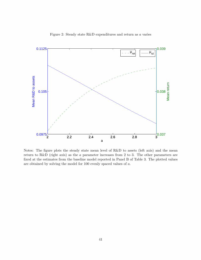
Figure 2: Steady state R&D expenditures and return as a varies

2 2.2 2.4 2.6 2.8 30.0975

0.105

0.1125

a

Mea

n R

&D

to a

sset

s

2 2.2 2.4 2.6 2.8 30.037

0.038

0.039

Mea

n re

turn

µ

rd µ

ret

Notes: The figure plots the steady state mean level of R&D to assets (left axis) and the meanreturn to R&D (right axis) as the a parameter increases from 2 to 3. The other parameters arefixed at the estimates from the baseline model reported in Panel B of Table 3. The plotted valuesare obtained by solving the model for 100 evenly spaced values of a.

41

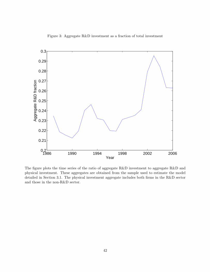
Figure 3: Aggregate R&D investment as a fraction of total investment

1986 1990 1994 1998 2002 20060.2

0.21

0.22

0.23

0.24

0.25

0.26

0.27

0.28

0.29

0.3

Year

Agg

rega

te R

&D

frac

tion

The figure plots the time series of the ratio of aggregate R&D investment to aggregate R&D andphysical investment. These aggregates are obtained from the sample used to estimate the modeldetailed in Section 3.1. The physical investment aggregate includes both firms in the R&D sectorand those in the non-R&D sector.

42