research and policy notes 3...2. key features of ifrs 9 for loan loss provisions the ifrs 9...

RESEARCH AND POLICY NOTES 3 Petr Polák, Jiří Panoš

The Impact of Expectations on IFRS 9 Loan Loss Provisions

RESEARCH AND POLICY NOTES


Petr Polák Jiří Panoš

3/2019

CNB RESEARCH AND POLICY NOTES The Research and Policy Notes of the Czech National Bank (CNB) are intended to disseminate the results of the CNB’s research projects as well as the other research activities of both the staff of the CNB and collaborating outside contributors, including invited speakers. The Notes aim to present topics related to strategic issues or specific aspects of monetary policy and financial stability in a less technical manner than the CNB Working Paper Series. The Notes are refereed internationally. The referee process is managed by the CNB Economic Research Division. The Notes are circulated to stimulate discussion. The views expressed are those of the authors and do not necessarily reflect the official views of the CNB. Printed and distributed by the Czech National Bank. Available at http://www.cnb.cz. Reviewed by: Péter Lang (Magyar Nemzeti Bank) Jan Sobotka (Czech National Bank)

Project Coordinator: Simona Malovaná

© Czech National Bank, December 2019 Petr Polák, Jiří Panoš


Petr Polák and Jirí Panoš ∗

Abstract

This paper describes the implementation of the IFRS 9 accounting standard into a macroprudential(top-down) stress-testing framework. It sets out to present a possible way of overcoming dataissues and discusses key assumptions which have an effect on the end results and which stresstesters should be aware of. According to the results, macroeconomic expectations play a crucialrole in the pass-through of impairment. The paper also presents evidence about the pro-cyclicalityof the IFRS 9 approach.

Abstrakt

Tato práce popisuje implementaci úcetního standardu IFRS 9 do makroobezretnostních (top-down)zátežových testu. Jejím cílem je prezentovat možný zpusob prekonání datových problému. Zabýváse klícovými predpoklady, které mají vliv na konecné výsledky a kterých by si testující meli býtvedomi. Výsledky ukazují, že pri transmisi znehodnocení hrají zásadní roli makroekonomickáocekávání. Práce rovnež prináší poznatky o procyklicnosti prístupu IFRS 9.

JEL Codes: E44, E62, G01, G21.Keywords: IFRS 9, impairments, loan loss provisions, macroprudential policy, stress test-

ing.

∗ Petr Polák, Czech National Bank and Charles University, Prague, [email protected]í Panoš, European Central Bank and Czech National Bank and University of Economics, Prague,[email protected] work was supported by grant VSE IG102029 and Polák acknowledge support from the Grant Agency ofCharles University (grant #1548119). The authors would like to thank Libor Holub, Jan Frait, Jan Sobotka, MarcelaGronychová, Péter Lang and Simona Malovaná for their comments and suggestions, which helped to improve thepaper significantly. The views expressed in this paper are those of the authors and not necessarily those of theCzech National Bank.

2 Petr Polák and Jirí Panoš

1. Introduction

International Financial Reporting Standard 9 – Financial Instruments (IFRS 9) was prepared by theInternational Accounting Standards Board (IASB) and issued in July 2014. It came into force inJanuary 2018 and has been the mandatory accounting framework for a significant number of EUbanks since then. This new accounting standard for loan loss provisioning represented a significantchange for the whole banking sector. It was created to replace the previous International AccountingStandard 39 (IAS 39) in the wake of the global financial crisis (GFC) with the aim to improve loanloss provisioning. Barth and Landsman (2010) argue that IAS 39 was one of the factors whichcontributed to the GFC, as it lacked forward-looking credit loss recognition. Bellotti and Crook(2012) explain that the underestimated credit risk present in the portfolio at that time was caused bythe mechanism of IAS 39, in which credit losses were recognised right after the impairment tookplace. This contributed to provisioning pro-cyclicality and underestimation of credit losses andrelated provisions, which in turn reduced banks’ resilience to shocks. IFRS 9, on the other hand,requires banks to base their credit losses on forecasts of the macroeconomic situation.

The motivation for the transition to IFRS 9 stems from the GFC. Pre-crisis IAS 39 loan loss pro-visioning was based on the incurred loss model, which caused delays in the recognition of creditlosses, widely labelled as “too little, too late”, such as in Laeven and Majnoni (2003). During thecrisis, a significant increase in fair value and impairment losses was observed. The recognition ofthese losses was perceived to have pro-cyclical features – banks did not have large enough buffersto cover the losses they made during the crisis, and had to form loan loss provisions from their di-minished profits in the subsequent downturn. Therefore, in 2009, the G20 called on the accountingstandard setters to “strengthen accounting recognition of loan-loss provisions by incorporating abroader range of credit information” and “improve accounting standards for provisioning” (OECD,2009).

In response to the G20, the Financial Stability Board (FSB) produced advice regarding the inter-action between accounting issues and pro-cyclicality based on the argument that recognising loanlosses at an earlier stage in the credit cycle might reduce pro-cyclicality. This included a recommen-dation to “reconsider the incurred loss model by analysing alternative approaches for recognisingand measuring loan losses that incorporate a broader range of available credit information” (FSB,2009). The new IFRS 9 standard is based on the expected credit losses (ECL) framework and aimsto be more forward-looking than its predecessor. Thus, according to IASB (2011), IFRS 9 shouldbe more transparent and less pro-cyclical. Optimally, banks would form provisions in good timeswhen they have sufficient profits, so that they can cover losses when an economic downturn comes.This should smooth the impacts of credit losses over the cycle.

It is expected that IFRS 9, if implemented properly, will help banks to recognise credit losses inadvance and thus avoid the kind of delays observed during the GFC. The idea of reducing pro-cyclicality is especially important for financial stability – banks are expected to provision appropri-ately at times of economic growth and should thus be more stable during crises. In addition, thehigher provisioning requirements should provide banks with an incentive to behave more cautiouslyand not to lend excessively during booms, since doing so should be more costly for them. In theory,banks should be able to calculate appropriate risk parameters with high precision given the detailedinformation they collect about their portfolios. On the other hand, they might have incentives tounderestimate the severity of adverse shocks in order to reduce the need to provision. Moreover,given the forward-looking nature of the ECL framework, expectations about future macroeconomicconditions play a crucial role in the new standard and might substantially affect loan loss provision-ing.

The Impact of Expectations on IFRS 9 Loan Loss Provisions 3

Stress tests have become an integral part of financial stability analysis since the last crisis. Borioet al. (2014) state that “given current (modelling) methodology, macro stress tests are ill-suited asearly warning devices”. The argument for this statement comes from the GFC, which was neitherpredicted nor indicated by the regularly conducted stress tests. We also agree with another asser-tion made by Borio et al. (2014) that “improvements in the performance of stress tests depend ona change in mindset”. To do the stress tests right, one has to revise the methodology regularly,incorporate advances in knowledge, and promptly adjust to new accounting and reporting rules.IFRS 9 is connected to one of the key risks in the banking sector – credit risk, so the change inthe accounting standard is being accompanied by gradual changes in regulatory reporting. Thereis no doubt that supervisory authorities themselves have to adapt in time and modify their existingstress-testing methodologies by integrating the new accounting rules properly, despite very oftenstill lacking sufficient data.

This paper presents the IFRS 9 methodology implemented in the Czech National Bank’s top-downmacroprudential stress test framework. As we discussed earlier, expectations about future economicconditions are one of the key drivers of loan loss provisioning under IFRS 9, so this paper also usesthis framework to show how different expectations might affect the timing of provisioning and anal-yses whether IFRS 9 differs in terms of pro-cyclicality from its predecessor IAS 39. To conductour analysis, we decided to employ the CNB’s workhorse top-down stress-testing framework aug-mented by an expectations layer, because this framework is directly tailored to testing the stabilityof the system as a whole and has all the necessary components already integrated into its structure.

The discussion about the pro-cyclicality of IFRS 9 is not new, but the academic evidence is scarce(see, for example, Gaffney and McCann, 2019; Abad and Suarez, 2017; Reitgruber, 2015). Therehave also been attempts to quantify the difference between the two standards; for instance, Krügeret al. (2018) simulate the bond portfolio. Domikowsky et al. (2014) analyse loan loss provisioningusing a sample of German banks and find counter-cyclical behaviour for specific provisions and noexplicit cyclical effects for general provisioning. Taking into account that at the time, German bankswere allowed to take a forward-looking approach to provisioning, this seems to be an importantfinding in support of the new IFRS 9 standard.

Cohen and Edwards (2017) describe the new provisioning approach from a more theoretical per-spective and conclude that it represents a step in the right direction. However, it is argued that theburden of the new standard might be substantial, especially for smaller institutions, given the com-plexity of the data which have to be maintained. From the supervisory perspective, new modelshave to be verified and well understood. The costs involved are significant and may raise concernsthat the new standard might be too demanding. Closer to our analysis is Seitz et al. (2018), whosimulate the expected credit loss model (IFRS 9) and compare the results with the incurred lossmodel (IAS 39). They suggest that ECL provisions tend to exceed IAS 39 provisions during timesof crisis and that there will not be a significant increase in counter-cyclical loan loss provisioning.

For our analysis, we decided to use a simplified banking sector model and to focus mainly on loans,since they usually represent the largest part of the banking sector’s balance-sheet exposure. Theresults calculated using the new IFRS 9 model will also be compared with the previous stress-testingframework using the incurred loss model described by Geršl et al. (2012). The first results underthe new methodology were presented in the Czech National Bank’s 2017/2018 Financial StabilityReport (CNB, 2018). However, this paper describes the methodology in more detail and emphasisesthe challenges stemming from different expectations about future economic conditions. To the bestof our knowledge, this paper is the first attempt to analyse the effects of different expectations onloan loss provisioning.


The paper is structured as follows: Section 2 focuses on the key features of IFRS 9, Section 3describes the credit risk models used in stress testing, Section 4 discusses the effect of expectationsand Section 5 gives conclusions.

2. Key Features of IFRS 9 for Loan Loss Provisions

The IFRS 9 accounting standard is primarily concerned with the classification and measurementof financial assets and liabilities and contains three significant building blocks: (a) recognition andmeasurement of financial assets and liabilities, (b) impairment and (c) hedge accounting. For top-down macroprudential stress testing, the first two are key.

Recognition and measurement deals with the problem of the classification and measurement offinancial assets for the balance sheet and profit & loss statement. The previous accounting standardIAS 39 is a rule-based approach with four classification categories of financial assets (loans andreceivables, FVPL, available for sale and held to maturity). The new accounting standard IFRS 9 isa principle-based approach with three classification and measurement categories of financial assets(amortised cost, FVPL and FVOCI). Expected credit losses are supposed to be recognised for allassets not measured at FVPL. For financial liabilities there are very few changes. Overall, the newapproach should be more robust regarding manipulation, more informative and, thanks to a short setof guidelines, also simpler. However, the real situation is more complicated, since the same assetscan be classified for similar firms differently (e.g. bonds) and the standard’s generality may lead toheterogeneous implementation across the industry.

Expected credit loss (ECL). The new approach to the classification of financial assets and liabilitiesalso directly affects loan loss provisioning. IAS 39 used the incurred loss framework, which requiredbanks to recognise credit losses only when evidence of a loss was apparent (BIS, 2017). This meansthat provisions were mainly created only after there were already known troubles with the financialasset. IFRS 9 has introduced the ECL framework for the recognition of asset impairment, whichmeans that banks have to determine the ECL at all times as from the initial recognition and holda proper amount of provisions. To determine the ECL, banks should not only use the availableinformation about past events, but also predict and forecast future developments. Because virtuallyevery loan has a certain probability of default (even if possibly very small), an appropriate ECLshould be associated with every loan since the time it was originated or acquired. If this probabilityor other factors change, the ECL should be adjusted accordingly, as this new approach aims to bemuch more forward-looking in order to ensure timely recognition of credit losses.

Impairment stages. Generally, there are three stages under IFRS 9 intended to reflect the deteriora-tion in the credit quality of a financial asset. It should be noted that the actual underlying probabilityof default does not directly determine whether the loan should be categorised as Stage 1 or Stage 2.In order to classify the loan as Stage 2, the probability of default has to increase significantly incomparison with the initial recognition. See subsection 2.1 for more details.

Stage 1 – Stage 1 covers all loans for which the credit quality has not deteriorated significantly sinceits initial recognition. For these loans, the 12-month ECL is recognised and the interest revenue iscalculated on the gross carrying amount.

Stage 2 – If a loan’s credit quality has deteriorated significantly since its initiation and the creditrisk is not very low, the loan is categorised as Stage 2. For loans in Stage 2, the lifetime ECLis recognised, but the interest revenue is still calculated on the gross carrying amount. Institutions


should evaluate regularly whether the credit quality has deteriorated and also determine what changewill be considered significant.

Stage 3 – If a loan has objective evidence of impairment, it is categorised as Stage 3. The lifetimeECL is recognised, as in Stage 2, but the interest revenue is calculated on the net carrying amount.It should be noted that from the regulatory perspective, Stage 3 (i.e. credit-impaired) loans are notthe same as non-performing loans. However, this approximation is usually quite suitable and doesnot cause any major distortion of the results. Such simplification can thus be part of stress-testingmethodologies, (see, for example, EBA, 2018).

12-month and lifetime losses. The ECL is recognised either for 12 months (Stage 1) or for thelifetime of the loan (Stage 2 and Stage 3). The lifetime ECL is the expected present value of theloss that is incurred if the borrower defaults at any time before the loan’s maturity. In general, thelifetime expected credit loss is calculated in four steps: (a) determine all the scenarios in which theloan defaults; (b) estimate the loss incurred in each scenario; (c) multiply the loss by the probabilityof the associated scenario; (d) discount and sum up all the results. This approach gives us the presentvalue of the probability-of-default weighted average of the credit losses. The 12-month ECL is theportion of the lifetime ECL which is associated with the time horizon of the next 12 months.

2.1 Significant Increase in Credit Risk

The important feature for the classification of financial assets under IFRS 9 is the change in creditrisk. A loan is reclassified from Stage 1 to Stage 2 if its credit risk deteriorates significantly (para-graph 5.5.9 of IFRS 9)1. The precise definition of significant increase in credit risk (SICR) is leftfor banks’ internal methodologies and might differ from bank to bank. For our top-down modellingperspective, we should understand what the main drivers of SICR are and how they can be modelledeffectively.

We identify three main determinants of SICR: (a) Macroeconomic environment. If the economicconditions deteriorate, uncertainty increases and an economic slowdown or downturn is expectedor even occurs, then the credit quality of assets is generally expected to deteriorate as well. Wecontrol for this in our approach.2 (b) Idiosyncratic factors. Banks observe behavioural changesin borrowers. Examples include an absence of regular income for retail and a sudden decrease inturnover for non-financial corporations. These are individual idiosyncratic characteristic stemmingfrom other sources than the macroeconomic environment and we are unable to model them properlyon the macro level. However, these effects can reasonably be expected to be diversified away onthe macro level and are beyond the scope of the top-down modelling framework. (c) Change inmodel estimates. This point might be valid for institutions without a sufficiently long customercredit history or which employ models that are not sufficiently robust.

It can be concluded that from the top-down perspective, the key driver of SICR is the macroe-conomic environment and SICR will tend to be strongly pro-cyclical. This logical conclusion isconfirmed by Gaffney and McCann (2019). SICR will cause credit exposures to shift from Stage 1to Stage 2, hence this ratio will be pro-cyclical too. For Stage 2 assets, lifetime expected creditlosses are required, so the loss provisioning will be related to the macroeconomic environment as

1 Instruments with low credit risk are excluded; see paragraphs 5.5.10 and B5.5.23 of IFRS 92 The approach used, however, does not perfectly grasp the entirety of the impact that macro variables could havethrough SICR, as the changes in the volume of Stage 2 exposures due to changes in macro variables will beproportional to the changes in the PD. However, the observed transitions to and from Stage 2 might be different ina normal economic situation and in a crisis, and they might not be proportional to the increase in the PD.


well. Thus, the ultimate key factor here is the accuracy of the predictions of future macroeconomicconditions which are then fed into the models. This factor can either promote early creation ofprovisions or cause later recognition of losses similar to IAS 39.

2.2 Interaction with Basel Requirements

In line with the Basel regulation, banks hold capital for unexpected losses, whereas expected lossesshould be covered by product pricing and loan loss provisions. Banks are also required to computethe regulatory expected losses. However, the Basel computations of expected losses differ from theaccounting perspective of IFRS 9. First, unlike in the case of IFRS 9, the time horizon for the Baselregulation is always 12 months. Second, while the regulatory expected losses should be through-the-cycle (TTC) and therefore rather independent of the macroeconomic cycle, IFRS 9 expected lossesshould be point-in-time (PiT) and thus explicitly take into account the current economic conditionsand forecasts (paragraph 5.5.17).

In general, provisioning affects CET1 capital through the profit & loss statement. Moreover, theBasel regulation specifies additional adjustments for possible shortfalls in provisioning. Para-graph 73 of Basel III states that if the regulatory expected loss exceeds the stock of provisions,the difference must be deducted directly from CET1. In the opposite situation, when the stock ofprovisions exceeds the regulatory expected loss, the excess may be added back to the Tier 2 capital.3

Ultimately, both measures affect CET1, and since IFRS 9 is expected to form provisions sooner andin a more sufficient manner compared to IAS 39, the new standard can be expected to be moreCET1-demanding than its predecessor at least in certain phases of the cycle.

To calculate IFRS 9 provisions, we need to identify, estimate and forecast an appropriate set of PiTrisk parameters and key macroeconomic variables (paragraphs 5.5.17 and BS.5.49 of IFRS 9). TheBasel requirements try to avoid pro-cyclicality using TTC risk parameters. The TTC values aimto be more independent of the macroeconomic risk factors. However, banks often use observedhistorical default rates (DF rates) to calibrate their PD models, and DF rates are naturally driven bythe macroeconomic situation. Hence, the TTC risk parameters are still indirectly determined by themacroeconomic factors, and a cyclical component is inherently present in the models, since banksproduce their estimates usually based on at least five years of historical observations according toArticles 180 and 181 of the CRR. Consequently, this approach might cause the risk weights tobehave pro-cyclically and will thus be replaced by a requirement to use data sets which include arepresentative mix of good and bad years. For more details, see, for example, Andersen (2011) orHeid (2007).

For IRB banks, which already had regulatory credit risk models in place, the adoption of IFRS 9was often considerably easier than it was for STA banks. This may raise the question of whetherthis new accounting standard could partially serve as an incentive for banks to switch from the STAto the IRB approach, which is generally less capital demanding (Behn et al., 2016; Mariathasan andMerrouche, 2014). For more information, see Prorokowski (2018), who contributes to the debate onthe suitability of the bank models used to meet the Basel requirement to calculate IFRS 9 expectedloss provisioning.

3 There is a limit of 0.6% of RWA; see paragraph 61 of Basel III.


3. Credit Risk Models in the Macro Stress-testing Framework

The majority of EU banks have adopted the new IFRS 9 accounting standard, which directly influ-ences the accounting recognition of credit risk, the most significant risk in the European bankingsector. Various approaches to credit risk stress testing are well described, for example, in Daniëlset al. (2017), Breuer and Summer (2017), Drehmann et al. (2010) and Buncic and Melecky (2013).However, in order to present the effects of expectations on the cyclicality of the IFRS 9 accountingstandard, we use the adjusted top-down macroprudential stress-testing framework of the CNB. Ourapproach to IFRS 9 modelling is originally based on the methodology developed at the ECB byGross et al. (2018) for applications within the EBA EU-wide stress-testing exercise. However, ourmodel is different in several important aspects. We assume the dynamic balance sheet approach,while employing our own data and satellite models for credit growth and risk parameters such asPD and LGD. Moreover, we have significantly re-worked the crucial loss rate estimation moduleof the model in order to efficiently utilise the full information contained in the transition probabil-ity matrix (TPM). We see our main contribution, however, in adding an expectations layer to themodel, which allows us to analyse different expectations about future developments and to assesstheir impact on loan loss provisioning and capital (see Section 4).

3.1 Credit Risk Framework under IAS 39

The previous framework for credit risk stress testing based on the IAS 39 principles was similaracross all central banks, so we use this approach as a benchmark measurement. Usually, the modelsplits the loan portfolio into segments (such as loans to non-financial corporations, households,governments, financial institutions etc.), and for every segment different growth rate, default rateand loss given default parameters are estimated. For the modelling purposes of this paper, we willuse just one theoretical segment, but the idea can be simply replicated for the other segments us-ing appropriately estimated parameters. For the regular top-down stress-testing exercise, we modelseveral portfolios for each bank in the system and then aggregate the results. However, for the pur-poses of this paper it suffices to model just one fictitious bank holding a theoretical, well-diversified,homogeneous4 portfolio of retail consumer loans.

To model the credit losses, we apply the dynamic balance sheet approach – the volume of grossloans (performing and non-performing together) over the period modelled is determined by a satel-lite model for the loan growth rate. To get the volume of performing loans, we subtract the non-performing loans volume from the gross loans volume. For each quarter, the volume of NPLs isgenerated according to the following set of equations:

GLt+1 = g ·GLt (1)NPLt+1 = NPLt +PDt+1 · (GLt −NPLt)−a ·NPLt (2)

PLt = GLt −NPLt (3)∆LLPt+1 = PDt+1 · (GLt −NPLt) ·LGDt+1−a ·LLPt +(PLt+1−PLt) ·PLcoverage (4)

where g is the gross loan growth parameter, NPL is the volume of non-performing loans, PL is thevolume of performing loans, GL is the volume of gross loans, PD is the probability of default, ∆LLPis the change in the volume of loan loss provisions, a is the NPL outflow parameter (write-offs) andPLcoverage is the average performing loans coverage ratio.4 The top-down modelling approach presented here implicitly assumes that the portfolios modelled are reasonablydiversified and homogeneous. Although this might not always be fulfilled in practice (especially when dealing withcorporate or institutional portfolios), it allows us to abstract from idiosyncratic factors and justifies the Markovapproach to the modelling of transitions.


Calculating the credit losses is therefore quite straightforward, as we have only one probabilityof default value determining the amount of newly defaulted loans. In this model, banks createprovisions equal to the realised losses. This means that the change in the NPL volume directlyaffects the profit & loss statement. We assume that all losses from the new NPLs are directlyrealised, so the loss is equal to the product of LGD and the new NPL volume. The loan lossesare then directly recorded in the profit & loss statement and hence directly affect the banks’ capital.Moreover, although banks were not required to provision for the expected losses, they usually held acertain amount of them, as reflected by the PLcoverage parameter. In general, loan loss provisioningunder the incurred loss model tends to be significantly pro-cyclical, as discussed, for example, byPool et al. (2015).

Even under the IAS 39 framework, we distinguish TTC and PiT values. The TTC values are usedfor the Basel capital requirements and the PiT values for the loan loss calculations.

3.2 Credit Risk Framework under IFRS 9

3.2.1 Probability of DefaultFor stress-testing purposes, the probability of default trajectory is usually produced by a satellitemodel. In general, central banks rarely have access to detailed loan-level data, so aggregate valuesare usually used. We were able to identify three different approaches to modelling the TTC andPiT values: (a) treat the PiT and TTC values completely separately and assume that the TTC valuesrequired for the Basel capital requirements are constant at a rating-class level, (b) use the TTCvalues reported by banks and then add a shock to get the PiT values, as at De Nederlandsche Bank(Daniëls et al., 2017), for example, or (c) take the PiT model values and calculate the TTC values asa long-term average. The last-mentioned approach is currently employed at the CNB (Geršl et al.,2012). This approach allows the TTC values to vary and is also in line with Article 181 of the CRRand the current EBA approach.

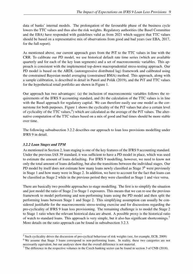
Figure 1: Probability of Default and Its Projection

0

2

4

6

8

10

12/15 12/16 12/17 12/18 12/19 12/20 12/21 12/22 12/23

(%)

Point-in-time (PiT) for the Baseline scenario Point-in-time (PiT) for the Adverse scenario

Through-the-cycle (TTC) for the Adverse scenario

Note: The chart depicts the historical default rates, projected PiT PD values and calculated TTC PD valuesfor the five-year horizon.

CNB (2018) discusses the lowering of IRB risk weights in the banking sector and states that thefurther we are from the crisis, the more the values from the post-crisis period dominate the input


data of banks’ internal models. The prolongation of the favourable phase of the business cyclelowers the TTC values and thus also the risk weights. Regulatory authorities (the Basel Committeeand the EBA) have responded with guidelines valid as from 2021 which suggest that TTC valuesshould be based on a representative mix of observations from good and bad years (see EBA, 2017,for the full report).

As mentioned above, our current approach goes from the PiT to the TTC values in line with theCRR. To calibrate our PD model, we use historical default rate time series (which are availablequarterly and for each of the key loan segments) and a set of macroeconomic variables. This ap-proach is consistent with the implemented top-down macroprudential stress-testing approach. OurPD model is based on the ARDL (autoregressive distributed lag) framework and calibrated usingthe constrained Bayesian model averaging (constrained BMA) method. This approach, along witha sample calibration, is described in detail in Panoš and Polák (2019), and the PiT and TTC valuesfor the hypothetical retail portfolio are shown in Figure 1.

Our approach has two advantages: (a) the inclusion of macroeconomic variables follows the re-quirements of the IFRS 9 accounting standard, and (b) the calculation of the TTC values is in linewith the Basel approach for regulatory capital. We can therefore easily use one model as the cor-nerstone for both purposes. Figure 1 shows the cyclicality of the PiT values but also a certain levelof cyclicality of the TTC values,5) which are calculated as the average of the PiT values. The alter-native computation of the TTC values based on a mix of good and bad times should be more stableover time.

The following subsubsection 3.2.2 describes our approach to loan loss provisions modelling underIFRS 9 in detail.

3.2.2 Loan Stages and TPMAs mentioned in Section 2, loan staging is one of the key features of the IFRS 9 accounting standard.Under the previous IAS 39 standard, it was sufficient to have a PD model in place, which was usedto estimate the amount of loans defaulting. For IFRS 9 modelling, however, we need to know notonly the total amount of loans defaulting, but also the transitions between the individual stages. OurPD model by itself does not estimate how many loans newly classified as Stage 36 were previouslyin Stage 1 and how many were in Stage 2. In addition, we have to account for the fact that loans canbe classified as Stage 2 while in the previous period they were classified as Stage 1 and vice versa.

There are basically two possible approaches to stage modelling. The first is to simplify the situationand just model the ratio of Stage 2 to Stage 1 exposures. This means that we can re-use the previousframework to model performing and non-performing loans using the PD model and then split theperforming loans between Stage 1 and Stage 2. This simplifying assumption can usually be con-sidered justifiable for the macroeconomic stress-testing exercise and for discussions regarding thepro-cyclicality of IFRS 9 loan loss provisioning. The remaining challenge is to model the Stage 2to Stage 1 ratio when the relevant historical data are absent. A possible proxy is the historical ratioof watch to standard loans. This approach is very simple, but it also has significant shortcomings.7

More details on the ratio approach can be found in subsubsection 3.2.3.

5 Such cyclicality drives the discussion of pro-cyclical behaviour of risk weights (see, for example, ECB, 2009)6 We assume that Stage 3 loans correspond to non-performing loans. In reality, these two categories are notnecessarily equivalent, but our analyses show that the overall difference is not material.7 The difference in the respective volumes in the Czech banking sector can be found in section 3 of CNB (2018).


The second possible approach is to model the whole transition probability matrix (TPM) and thecorresponding flows between the individual stages. This approach is more precise and providesadditional information as well. The TPM in our approach is a time-variant stochastic matrix ofa discrete-time, discrete-state-space inhomogeneous Markov chain, and we use the subscript t tohighlight that the TPM elements are not constant over time. T PXY,t represents the transition prob-ability from Stage X to Stage Y at time t. In addition, some methodologies (e.g. EBA, 2018) addthe “no-cure from Stage 3” assumption, which means that loans can never recover once classifiedas Stage 3. This assumption makes the modelling considerably easier, since we are not required tomodel the transition probabilities from Stage 3 back to Stage 1 and Stage 2 and we do not have todeal with double defaults over the period modelled. Thus, in our approach we too assume no cures(and no repayments) from Stage 3, which consequently becomes an absorbing state of the Markovchain, and the number of parameters which need to be modelled is therefore reduced by two (seeTable 1).

Table 1: TPM of Markov Chain

From/To Stage 1 Stage 2 Stage 3Stage 1 T P11,t = 1−T P12,t −T P13,t T P12,t T P13,tStage 2 T P21,t T P22,t = 1−T P21,t −T P23,t T P23,tStage 3 T P31,t = 0 T P32,t = 0 T P33,t = 1

Note: Blue cells represent matrix elements which need to be modelled.

To get the volume of loans in each stage under the constant balance sheet approach, we can simplymultiply the vector of current volumes in each stage by the corresponding TPM to get the volumesin each stage at the beginning of the next period, as in equation 5. The general approach underdynamic balance sheets and further details are described in subsubsection 3.2.4.

ExpS1,t+1ExpS2,t+1ExpS3,t+1

T

=

ExpS1,tExpS2,tExpS3,t

T

·

T P11,t T P12,t T P13,tT P21,t T P22,t T P23,tT P31,t T P32,t T P33,t

(5)

3.2.3 Using S1/S2 Ratio to Model Loan StagesAs the starting point for the modelling under the baseline scenario, we can use the current ratio ofStage 2 to Stage 1 loans that banks report within the regulatory reporting. However, our main aimis to model the path under the adverse scenario. To achieve that, we assume that the ratio of Stage 2to Stage 1 exposures would double over the stress period. As a benchmark to derive this relativeincrease, we use the ratio of standard to watch loans during the GFC. The predicted probabilities ofdefault from the current model can be used without changes. In the new context, they represent thetotal transition from Stage 1 and Stage 2 to Stage 3. Nevertheless, modelling of the whole TPM isnecessary, as it allows us to model the transitions between the different stages using the individualtransition probabilities, and it is also important for more rigorous modelling of the ECL. Therefore,we reject the S1/S2 ratio approach in favour of the approach detailed in the next subsection, whichhas the potential to deliver more precise and informative results.

3.2.4 TPM Modelling MethodologyAs mentioned above, the TPM in our framework is a stochastic matrix which is not constant overtime and carries information about the probabilities of transition between the IFRS 9 stages. Sincewe are limited by a lack of historical data availability, we do not model each T Pxy separately. Instead,


we use the initial value of the TPM, the constrained-BMA PD model (Panoš and Polák, 2019) anda set of bridge equations to infer the values of the matrix in each period. Therefore, to get thetransition probabilities we use three different ingredients for each loan segment: (a) the startingpoint values of the TPM, (b) the projected PiT PD trajectories from the PD satellite model and (c) apair of linear bridge equations with suitably estimated parameters. First, the starting values of theTPM have to be estimated using either the regulatory reporting data or some other relevant datasource, such as the bottom-up supervisory stress testing. Afterwards, the trajectories of T P13 andT P23 can be estimated using distance-to-default (DD) transformation. Finally, the T P12 and T P21trajectories are calculated using the T P13 and T P23 values acquired in the previous step. To obtainthe remaining T P11 and T P22 values on the main diagonal of the TPM, we can utilise the fact that theTPM is a stochastic matrix and hence these values can be calculated such that the sum of each rowis equal to one. We assume Stage 3 to be the absorbing state with no recovery rates, hence T P31 andT P32 are both equal to zero and T P33 equals one. The general DD transformation is mathematicallyexpressed as:

DD :=−Φ−1 (PD) (6)

where Φ−1 is the inverse cumulative distribution function (CDF) of the standard normal distribution.This transformation was first defined by Merton (1974). In the context of the original model, itmeasured how many standard deviations of the asset probability distribution a given firm is distantfrom bankruptcy. Among market practitioners, it is widely agreed that the distance to default is auseful measure for assessing the credit risk of a non-financial corporation (Chan-Lau and Sy, 2007).From the mathematical perspective, it is virtually equivalent to the probit transformation. The mainadvantage of this transformation is that we are no longer limited to the [0,1] interval for PD, but wehave the whole set of real numbers. In addition, the non-linear nature of the transformation leads tosmaller values of PD being stressed more than larger ones. That further promotes the conservativenature of the model, which is fully in line with the spirit of the top-down macroprudential stress test.Naturally, the inverse transformation is used to get the projected values back to the [0,1] interval:

T P13,Ti = Φ

(Φ−1 (T P13,T0

)+Φ

−1 (PDTi

)−Φ

−1 (PDT0

))T P23,Ti = Φ

(Φ−1 (T P23,T0

)+Φ

−1 (PDTi

)−Φ

−1 (PDT0

)) (7)

At this point, we are in a position to obtain the T P12 and T P21 trajectories. Empirical observationsmade by Gross et al. (2018) suggest that in the DD space, linear relations exist between T P12 andT P13 and T P21 and T P23, which can be expressed as a regression line model:

Φ−1 (T P12,t

)= α +βΦ

−1 (T P13,t)+ εt ,∀t

Φ−1 (T P21,t

)= γ +δΦ

−1 (T P23,t)+ωt ,∀t

(8)

We a priori expect a positive correlation between T P12 and T P13 (i.e. β > 0) and a negative correla-tion between T P21 and T P23 (i.e. δ < 0). Unfortunately, only very limited data series from regulatoryreporting are available to estimate the coefficients β and δ at the moment. For the time being, wetherefore resort to the values estimated for the Czech Republic in the EBA stress-testing exercise,which we periodically update using Bayesian regression principles. For the purposes of our analysiswith only one hypothetical loan segment, we use approximately average values of these coefficients,i.e. β = 0.5 and δ =−0.5 The final projections of the T P12 and T P21 values are then obtained usingthe starting point values, the estimated coefficients β and δ , the previously obtained trajectories ofT P13 and T P23 and inverse DD transformation:


T P12,Ti = Φ

(Φ−1 (T P12,T0

)+ β

(Φ−1 (T P13,Ti

)−Φ

−1 (T P13,T0

)))T P21,Ti = Φ

(Φ−1 (T P21,T0

)+ δ

(Φ−1 (T P23,Ti

)−Φ

−1 (T P23,T0

))) (9)

As mentioned before, the rest of the TPM is calculated such that it satisfies the definition of astochastic matrix, i.e. the sum of the row values is equal to one. There is no mechanism in thisapproach to ensure that the sum of the modelled parameters T P12 +T P13 and T P21 +T P23 is lessthan or equal to one. If the sum is actually greater than one, the transition probability on the maindiagonal is then set to zero and the off-diagonal entries are normalised (ECB, 2017).

The initial TPM for the period is shown in Table 2. With the initial TPM and its evolution over timein our hands, we can calculate the loan volumes in each stage for every loan segment and time step,as described in the following part of this paper. The data limitations that prevent us from modelling

Table 2: Sample TPM

From/To Stage 1 Stage 2 Stage 3 ∑

Stage 1 96.8 1.8 1.4 100.0Stage 2 11.7 78.0 10.3 100.0Stage 3 0.0 0.0 100.0 100.0

Note: Values are shown in percentages.

the transitions between stages directly will hopefully soon perish. Since the introduction of IFRS 9,banks have been paying more attention to instrument classification, and various pieces of informa-tion regarding the stage transitions are reported to supervisory authorities. More detailed data areavailable to supervisors thanks not only to IFRS 9, but also to projects such as AnaCredit.8 How-ever, it will take several years (maybe even decades) before sufficient-quality time series from thesesources become available, i.e. before the series are long enough to contain a period of economicdownturn.

3.2.5 Credit Growth, Loan Volumes and StagesFor each loan segment, the flows between stages have to be modelled for the whole stress-testingperiod. These flows are governed by the transition probability matrix and its evolution over time(for the derivation of the TPM, see subsubsection 3.2.4).

Determining the loan volumes in the individual stages one time step ahead is divided into two steps.First, the corresponding TPM is applied to the current loan volumes. Then, the new loans are addedto Stage 1 and the loans that banks write off are subtracted from Stage 3. Together with the written-off loans, we also remove the appropriate amount of provisions. This approach allows us to use thedynamic balance sheet and produces a more realistic ratio of performing to non-performing loans.9

Formally, the loan volume in each stage is given by:8 AnaCredit is a project to set up a data-set containing detailed information on individual bank loans in the euroarea, harmonised across all member states. “AnaCredit” stands for analytical credit datasets. It was set out inRegulation (EU) 2016/867 of May 2016 (ECB/2016/13).9 We prudentially assume no repayments from Stage 3, which can be reduced only via write-offs. However, itis also implicitly assumed there are no repayments from Stage 2. This assumption would not hold in reality –unfortunately, our current credit growth satellite model does not allow us to distinguish between new credit (inflowto Stage 1) and repayments (outflow from Stage 1 and Stage 2), hence we consider this to be one of the areas forpotential improvement.


ExpS1,t+1ExpS2,t+1ExpS3,t+1

T

=

ExpS1,tExpS2,tExpS3,t

T

·

T P11,t T P12,t T P13,tT P21,t T P22,t T P23,t

0 0 1

+CCt ·Expt +WOt ·ExpS3,t

0−WOt ·ExpS3,t

T

(10)

where ExpSs,t represents the exposure at time t in Stage s; T Pi j,t represents transition from Stage ito Stage j at time t; CCt is the credit growth of the total gross exposure (Expt) at time t; and WOt isthe write-off parameter at time t.10 It is important to emphasise that the credit growth captured byCCt is lowered in each period by the outflow of Stage 3 exposures captured by WOt . However, sincewe target credit growth at the CCt level, we have to add the volume that has been written off. This isa rather technical issue based on an understanding of the CCt parameter, specifically that the growthof the whole stock of exposures is a more relevant financial stability indicator and is also easier tomodel over time.

3.2.6 Loan Loss Provision ModellingThe next step in IFRS 9 expected loss modelling is to estimate the loss rates for the individual stages.For exposures moving to Stage 3, we use the loss given default (LGD) parameter, as we assume thatthe losses are realised immediately and that no cure from S3 is possible. It follows that the totalamount of Stage 3 provisions depends on the previous LGDs and corresponding exposure amountstransitioning to Stage 3. For exposures in Stage 1 and Stage 2, we need the 12-month loss rate (12MLR) and the lifetime loss rate (LT LR) respectively. Last but not least, we need the average residualmaturity for each credit segment. The residual maturity data are taken from regulatory reportingand the bottom-up supervisory stress tests. For the LGD estimation, we use a satellite model and,once again, information from the bottom-up stress tests, where banks provide their LGDs and otherrisk parameters. The LGD satellite model is defined in detail by Geršl et al. (2012).

IRB banks also report their LGD values within regulatory reporting. Some central banks (see, forexample, Daniëls et al., 2017) use these values in their stress-testing frameworks. These values arereported according to the Basel regulation and should be interpreted as “downturn” LGDs, meaningthat estimated losses should be appropriate for an economic downturn. The situation is in fact anal-ogous to the PD case discussed earlier, as here again we require PiT values for the computation ofcredit losses and provisioning and different regulatory values for the capital adequacy calculations.Similarly to PD PiT, the LGD PiT values are expected to be pro-cyclical, as collateral value tendsto be negatively affected by recessions (see Figure 2).

12-month and Lifetime Loss Rates It is a well-known property of an inhomogeneous Markovchain that the elements of the product of the chain’s N subsequent TPMs represent the probabilitiesthat a chain which originally started in a state given by a specific row is, after N periods, in a stategiven by a specific column. From the absorbing property of Stage 3, it can be concluded that theelement at position (1,3) (respectively (2,3)) of the product of N subsequent TPMs gives us theprobability that an exposure which initially started in Stage 1 (Stage 2) moved to Stage 3 from anyother stage in the N-th period at the latest. From that, it can be further derived that the differencebetween the elements at position (1,3) (respectively (2,3)) of the multiples of N and N-1 subsequentTPMs gives the probability of an exposure initially starting in Stage 1 (Stage 2) moving to Stage 3from any other stage exactly in the N-th period. Let us denote these probabilities as T P1−3

N,Tifor

10 In reality, Stage 3 exposures can also be reduced through loan sales. We abstract from loan sales in our modellingapproach.


exposures being in Stage 1 at time Ti and T P2−3N,Ti

for exposures being in Stage 2 at time Ti. The 12MLR is then calculated as:

LRS112M,Ti

=4

∑k=1

[(1

1+ rTi

)k·EADTi−1+k ·LGDTi−1+k ·T P1−3

k,Ti

]/EADTi (11)

where r stands for the interest rate in the specific loan segment and EAD for the exposure size. Thus,LRS1

12M,Tirepresents the discounted value of the expected credit losses for exposures in Stage 1 in

the next 12 months (four quarters) expressed as a percentage of the original exposure value, whichmeets the IFRS 9 requirements.

Similarly, we model the lifetime LR as:

LRS2LT,Ti

=M

∑k=1

[(1

1+ rTi

)k·EADTi−1+k ·LGDTi−1+k ·T P2−3

k,Ti

]/EADTi (12)

where M represents the residual maturity expressed in quarters in the given loan segment. LRS2LT,Ti

represents the discounted value of the expected credit losses for exposures in Stage 2 from Ti untilmaturity expressed as a percentage of the original exposure value, which again meets the IFRS 9requirements.

For simplicity, we assume that the EAD decreases linearly up to maturity. The LGD values alsodecrease linearly, but cannot fall below a defined threshold representing the costs of litigation andother relevant fixed costs associated with a default event. The transition probabilities T P1−3

k,Tiand

T P2−3k,Ti

are also important drivers of the ECL in formulae 11 and 12. For many loan segments, thematurities stretch beyond the modelling horizon, so we have to determine the long-term averagesto which the both the baseline and adverse values of the risk parameters converge after the stress-testing period. These long-term averages can be calculated using historical time series (if available)or as weighted averages of the values from the baseline and adverse scenarios, or can be set byexpert judgement. We assume a six-year convergence period, after which the risk parameters stayflat.

Figure 2 shows the LGD path and Figure 3 the loss rate paths for the given scenarios. As mentionedabove, we again differentiate between the LGDs used for the capital requirements and the PiT LGDsused for the IFRS 9 ECL provisions.

Since we have already discussed all the necessary features required to calculate the ECL and theassociated loan loss provisions in the IFRS 9 framework, the next part of this paper forms a stylisedportfolio and applies the methods and calculations introduced above to show how different expec-tations about future macroeconomic conditions might influence provisioning and ultimately affectcapital adequacy, which is one of the key measures of banks’ stability.


Figure 2: LGD

0

10

20

30

40

50

60

70

80

12/16 12/17 12/18 12/19 12/20 12/21 12/22 12/23

(%)

LGD Baseline LGD Adverse

Note: The chart depicts the LGD path under the baseline and adverse scenarios for the sample portfolio.

Figure 3: Loss Rates

0

1

2

3

0

5

10

15

20

25

30

12/18 12/19 12/20 12/21 12/22 12/23

(%)(%)

Life-time loss rate (LT LR) Baseline Life-time loss rate (LT LR) Adverse

12-month loss rate (12M LR) Baseline (rhs) 12-month loss rate (12M LR) Adverse (rhs)

Note: The chart depicts the LR and 12M loss rate paths under the baseline and adverse scenarios for thesample portfolio.


4. Expectations and Impact on Capital

4.1 Stylised Credit Portfolio

This section presents a hypothetical retail loan portfolio and calculates the impact of macroeco-nomic scenarios under different expectations about future conditions. This allows for a compre-hensive comparison of the impact and for a discussion regarding the pro-cyclicality of the IFRS 9accounting standard. We first make several assumptions that are inherently embodied in the stan-dard macro-stress-testing exercise and add the macroeconomic scenarios for which the impact ofthe new accounting standard will be calculated. The period modelled is five years, and the evolutionof the variables is computed on a quarter-by-quarter basis. We approach the portfolio from the top-down perspective, so homogeneity is assumed and aggregate values are used. We assume the IRBmethodology for calculating regulatory capital and consider only one homogeneous retail portfolioof consumer loans.11

Regarding the scenario design, our main motivation is the time span in which we want to demon-strate the effects of the accounting framework, while maintaining basic economic principles andapplying a severe yet plausible economic downturn. In the adverse scenario, the economy follows apositive trend in the first six quarters and is then hit by a sudden crisis. This crisis lasts for roughlythree years, which means that within the five-year horizon we are also able to model the beginningof an economic recovery. The final results are presented for two macroeconomic scenarios (base-line and adverse) and three different types of expectations, and are compared among themselvesand with the previous IAS 39 approach. We consider the same starting point values and long-termaverages for all calculations to ensure that any differences in the results are solely determined bythe different approaches to expectations.

Table 3: Stylised Credit Portfolio

Stage Volume Provisions Coverage ratio (%) Risk weightStage 1 892 4 0.5 47.0Stage 2 61 6 10.4 47.0Stage 3 47 34 72.3 50.0

Note: The table provides starting-point information about the stylised portfolio. We assume that loans areretail consumer loans, split into stages, and that the coverage ratios are proportionately equivalent tothose of the Czech banking sector. For the risk weight for defaulted exposures, we assume that thedifference between LGD and ELBE is 4% and constant over time.

Table 3 summarises the stylised credit portfolio, which has a nominal value of 1,000 units, and weassume that there are no other assets. We use the S1-S2-S3 ratio from the Czech banking sector,resulting in 892 units in Stage 1, 61 units in Stage 2 and 47 units in Stage 3. Based on the evidencefrom regulatory reporting, we set Stage 3 loans equal to non-performing loans and to loans in defaultaccording to CRR.12 For the coverage ratios’ starting values (i.e. the stock of provisions for eachstage divided by the associated loan volume), we again use values from the Czech banking sector.The coverage ratios for Stage 1, Stage 2 and Stage 3 loans are 0.5%, 10.4% and 72.3% respectively.The starting-point risk weight (RW) of 47.0% for non-defaulted loans and 50% for defaulted loansimplies an initial risk exposure amount (REA) of 474.4 units. We assume a starting capital ratio of

11 In the actual CNB stress-testing exercise, we distinguish between loan segments with respect to FINREP report-ing.12 These three sets are generally not identical, but the difference tends to be sufficiently small.


20%, which implies 94.9 units of regulatory capital, and we further assume that banks will earn 7.5units quarterly.13 If banks’ capital ratio is higher than the initial level of 20% in any given period,the rest is paid out as dividends. This assumption should lead to higher resilience for banks that usethe forward-looking IFRS 9 approach and thus conserve their capital in good times in comparisonto those which do not take expected future developments into account.

We employ the dynamic balance sheet approach with the credit growth path shown in Figure 4.Moreover, we work under the assumption that banks reduce their lending volume during the crisis,but the riskiness of new loans is the same as that of the current stock, so the homogeneity of theportfolio is maintained. In reality, however, banks tend to loosen their lending standards during pe-riods of economic growth and tighten them during downturns (Hromadkova et al., 2018). Rigorousmodelling of such behaviour is quite complex and therefore we leave aside this phenomenon andinstead prefer to work with conservative values of the risk parameters.

Figure 4: Credit Growth in the Scenario

-4

-2

0

2

4

6

8

12/15 12/16 12/17 12/18 12/19 12/20 12/21 12/22 12/23

(%)

Baseline Adverse

Note: The chart depicts the credit growth path under the baseline and adverse scenarios. The scenario-conditional trajectories are produced by a dedicated CNB satellite model.

In the stress-testing exercise, the scenarios are the key drivers of the final results. Since IFRS 9 aimsto be forward-looking and we need to calculate the lifetime expected losses for Stage 2 loans, wehave to make assumptions about the evolution of key variables beyond the stress-testing horizon.Furthermore, we need data regarding the residual maturity of the loan portfolio. Both of these issueswere discussed earlier in this paper.

Credit losses are driven by loan defaults. Under the IAS 39 modelling approach, the projectedPD is the only variable needed to determine the volume of newly defaulted loans. For simplicity,we assume that provisions are created in the same amount as the actual loan losses (defined asthe volume of newly defaulted loans times the loss given default). Under the IFRS 9 modellingapproach, provisions equal to the ECL should be created even for performing loans, which means

13 This assumption is based on an ROA equal to 3%.


that the stock of provisions has to be modelled for each stage and each time period. The expectedlosses differ between the individual stages, so the associated stocks of provisions differ as well. Inthe IAS 39 framework, there are only performing loans and NPLs. For IFRS 9, however, we haveto split performing loans into Stage 1 and Stage 2. This split is crucial, and the possible ways ofdoing so were discussed in subsubsection 3.2.2. In the following part, we will use both approachesand compare them.

4.2 Expectations about Future Developments

According to IFRS 9, current and expected macroeconomic conditions should be taken into accountwhen determining the ECL. Estimates of current economic indicators are usually available, butforecasting future developments is often problematic. Not only are the models used to predict thefuture imperfect, but the magnitude of crises is often underestimated, as shown by An et al. (2018).The following analysis compares different types of expectations about macroeconomic conditionsand their impact on provisioning.

Figure 5: Real GDP Growth Forecast and Possible Crisis Timing

-6

-4

-2

0

2

4

6

12/15 12/16 12/17 12/18 12/19 12/20 12/21 12/22 12/23

(%)

Baseline Adverse

Note: The chart shows the assumed path of real GDP growth. The blue line represents the baseline scenario,while the red line shows the path of the economic downturn in the adverse scenario.

We have already shown how 12-month and lifetime loss rates are calculated in our model, but thekey driver in these calculations is expectations about future developments. One possible approachis perfect foresight. Perfect foresight means that all the information is available at any time, andentities know precisely when the next crisis will arise and how long and severe it will be. On theone hand, this assumption is obviously very strong and rather unrealistic. On the other hand, for thetop-down stress-testing exercise it makes the situation easier, because the stress-testing scenariosare transferred directly into the estimated risk parameters from the beginning of the test. This wasone of the reasons behind the emergence of IFRS 9 accounting – banks are supposed to create loanloss provisions in good times, before a crisis hits them. However, if we want to achieve and analysecloser-to-reality behaviour, we can relax this assumption and try to model how different expectationsand applications of the IFRS 9 principles can affect banks. For the purposes of this paper, we assume


a crisis (negative GDP growth) that comes a year and a half after the beginning of the modellingperiod and lasts approximately three years (see Figure 5 for a graphical representation).

For the crisis given by our scenario, we test three types of expectations (a) the perfect foresightapproach, where all the information is known from the beginning, (b) the optimistic approach,where banks always believe that the situation will start to revert to the baseline scenario in the nextperiod and (c) the Bayesian approach, where banks’ expectations are gradually adjusted to reflectthe inflow of new information.

The perfect foresight approach assumes that the exact path of the crisis is known to all entitiesat the beginning of the stress test. Under perfect foresight, provisioning tends to be smoother.Therefore, banks are better able to manage the crisis, since they have enough provisions on theirbalance sheets before the crisis, as they conserve revenues in good times to cover their losses in badtimes. However, in a real stress situation, no bank will have perfect knowledge of the future, whichmeans IFRS 9 provisions might behave differently than under the perfect foresight approach.

The optimistic approach is our label for the second type of expectations under consideration. Itassumes that at each time step of the downturn period, banks expect the situation to start convergingtowards the baseline path in the next period. Figure 6 shows the optimistic approach to expectationsabout the path of real GDP over time.

Figure 6: Real GDP Growth Rate Forecast Based on Optimistic Expectations about FutureDevelopments

-6

-4

-2

0

2

4

12/18 12/19 12/20 12/21 12/22 12/23

(%)

Assumed GDP development in the exercise

Expected GDP according to the optimistic approach

Note: The dashed lines represent expectations about the real GDP growth path at any given time. It isalways assumed that the economic situation will start improving in the next period and quicklyconverge towards the baseline scenario.

The Bayesian approach is our label for the third type of expectations about future developments. Inthis case, banks can see as far as two periods ahead and evaluate the currently available informationabout economic developments. We start in good times, so banks’ prior beliefs incline towards the


baseline scenario and then gradually switch to the adverse one as new information arrives. Theexpectations about real GDP in the Bayesian approach are depicted in Figure 7.

Figure 7: Real GDP Growth Rate Forecast Based on Bayesian Expectations about FutureDevelopments

-6

-4

-2

0

2

4

12/18 12/19 12/20 12/21 12/22 12/23

(%)

Assumed GDP development in the exercise

Expected GDP according to the bayesian approach

Note: The dashed lines represent expectations about the GDP growth path at any given time. Banks use theavailable information up to two periods ahead to gradually update their beliefs regarding the scenario.

From our perspective, the alternative approaches to expectations are closer to reality than the perfectforesight approach, as banks do not possess crystal balls and in general might be tempted to postponeprovisioning to the future in the hope that a more serious downturn will never come.

4.3 Impairment Creation

Different paths of the loss rate parameters and the stock of provisions are calculated for each of theselected approaches to expectations. The techniques described in subsubsection 3.2.6 are used tosimulate the projected paths conditional on the presented scenarios and approaches to expectations.One of the key results is the path of provisions, as shown in Figure 8. The following paragraphs aimto highlight the differences between the presented approaches.

The provisions created according to IAS 39 depict the losses suffered by banks under the previousaccounting framework and also serve as a benchmark for all the IFRS 9 framework results. Thepath is based on the losses already incurred and is therefore strongly connected to the way the crisisunfolds in the hypothetical retail credit portfolio. No substantial buffers are created prior to thecrisis in this approach.

Under the perfect foresight approach, one can easily observe the gradual increase in provisioningahead of the crisis, as banks know with certainty that the crisis is approaching. The perfect foresightensures that there are more provisions at the dawn of the crisis, and the provisions created to coverperforming loans (Stage 1 and Stage 2) can be used in later stages to cover the losses arising fromloans that become non-performing (Stage 3) in the course of the crisis.


In the case of the optimistic approach, banks provision much less for performing loans (especiallyprior to the crisis), as the economic situation perceived by banks is always more optimistic thanthe actual situation prescribed by the scenario at each time step. Since the macroeconomic path isultimately the same in all the approaches, this leads to banks postponing the creation of provisions.This causes the provisioning to be more pro-cyclical and, in the later stages, similar to IAS 39, asbanks need to provision for the new non-performing loans, for which the ECL and the associatedprovisions were previously underestimated.

Figure 8: Loan Loss Provisions Creation

0

4

8

12

16

20

12/18 12/19 12/20 12/21 12/22 12/23

(units)

Baseline Adverse Perfect foresight Adverse Bayesian approach

Adverse Optimistic approach Adverse IAS39

Note: The figure shows the quarterly creation of loan loss provisions for each expectation type for the sameunderlying scenario. PF stands for perfect foresight.

One of the potential pitfalls of IFRS 9 is captured by the Bayesian approach. In this case, banksrealise the true depth and length of the crisis too late and so are forced (either internally or bysupervisors, auditors or other authorities) to create a vast amount of additional provisions duringthe downturn, when their revenues are diminished. This leads to a severe “cliff effect” with a largeimpact on banks’ overall capital position. This potentially causes a credit crunch with spillovers tothe real economy, and threatens the stability of the system.

Hence, based on an examination of Figure 8, it seems that perfect foresight is the key ingredientof IFRS 9, one which can truly reduce the need to form loan loss provisions during recessions. Ifbanks knew about the crisis in advance and behaved accordingly, IFRS 9 would without doubt beless pro-cyclical than the previous standard.

The pre-crisis period and recovery period actually highlight the biggest differences between theperfect foresight IFRS 9 and IAS 39. We observe that at the end of the crisis, banks can startto release provisions created for performing loans and use them to cover the losses caused by theincreased inflow of non-performing loans. Such behaviour, where the creation of provisions ishigher before the start than at the end of the crisis, is desirably counter-cyclical. In addition, bankspay the least dividends, as they use their profits in good times to create a cushion for bad times(this is discussed in more detail in the following section). However, the assumption of perfect


foresight can effectively only be applied in stress-testing exercises. In reality, banks do not have aprecise knowledge of either the timing or length and depth of the crisis. In addition, the majorityof macroeconomic forecasts and equilibrium models rarely predict deep or prolonged crises. Wetherefore expect banks’ real-world behaviour to resemble our alternative approaches to expectationsrather than the perfect foresight approach.

4.4 Basel Requirements and CET1 Capital Impact

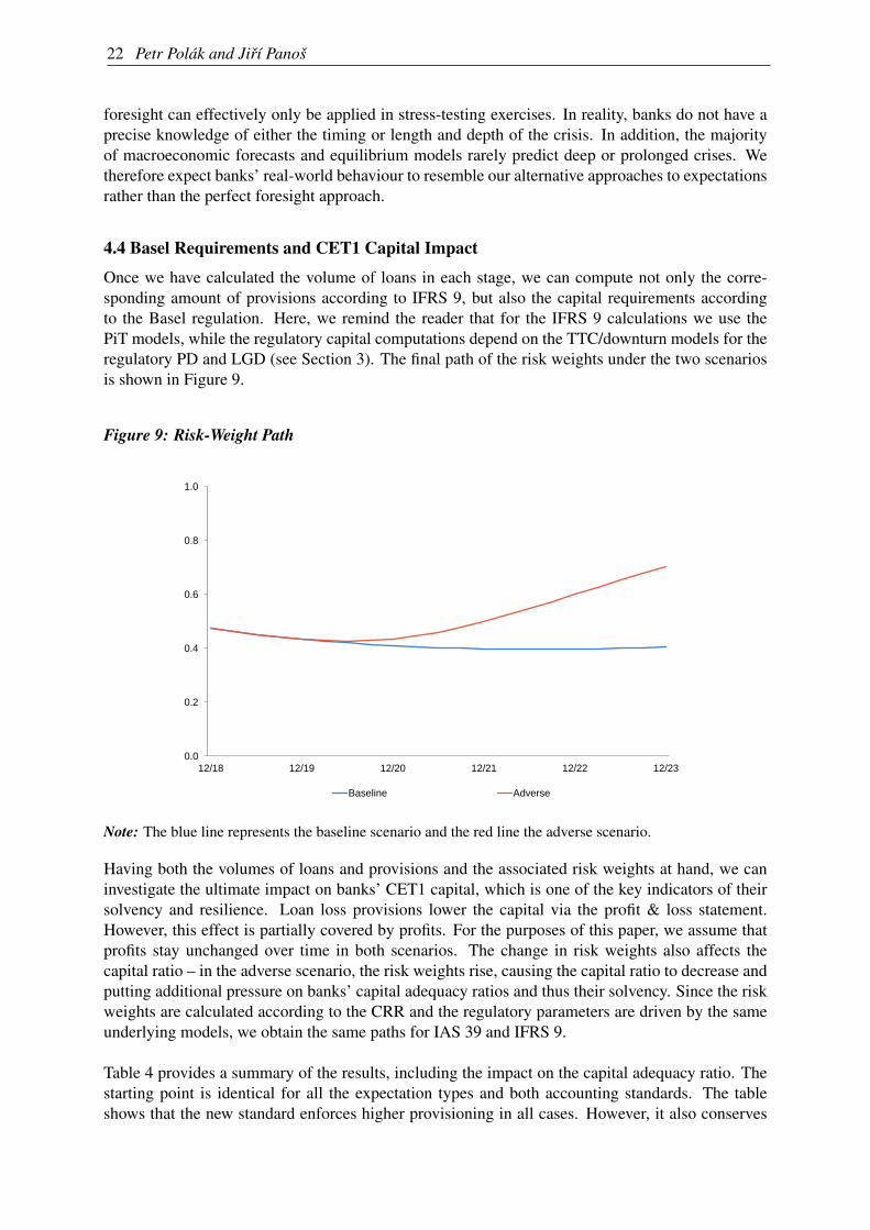
Once we have calculated the volume of loans in each stage, we can compute not only the corre-sponding amount of provisions according to IFRS 9, but also the capital requirements accordingto the Basel regulation. Here, we remind the reader that for the IFRS 9 calculations we use thePiT models, while the regulatory capital computations depend on the TTC/downturn models for theregulatory PD and LGD (see Section 3). The final path of the risk weights under the two scenariosis shown in Figure 9.

Figure 9: Risk-Weight Path

0.0

0.2

0.4

0.6

0.8

1.0

12/18 12/19 12/20 12/21 12/22 12/23

Baseline Adverse

Note: The blue line represents the baseline scenario and the red line the adverse scenario.

Having both the volumes of loans and provisions and the associated risk weights at hand, we caninvestigate the ultimate impact on banks’ CET1 capital, which is one of the key indicators of theirsolvency and resilience. Loan loss provisions lower the capital via the profit & loss statement.However, this effect is partially covered by profits. For the purposes of this paper, we assume thatprofits stay unchanged over time in both scenarios. The change in risk weights also affects thecapital ratio – in the adverse scenario, the risk weights rise, causing the capital ratio to decrease andputting additional pressure on banks’ capital adequacy ratios and thus their solvency. Since the riskweights are calculated according to the CRR and the regulatory parameters are driven by the sameunderlying models, we obtain the same paths for IAS 39 and IFRS 9.

Table 4 provides a summary of the results, including the impact on the capital adequacy ratio. Thestarting point is identical for all the expectation types and both accounting standards. The tableshows that the new standard enforces higher provisioning in all cases. However, it also conserves


more capital, since the payout of dividends is highest under IAS 39. These observations favourIFRS 9, as the higher amount of provisions and increased capital conservation should strengthenbanks’ stability during a downturn. However, clearly only the perfect foresight approach ensures asignificant improvement in terms of conservation, as it retains almost six units of capital more incomparison with the other approaches based on IFRS 9 and almost seven units of capital more incomparison with IAS 39.

Table 4: Summary of Results

Expectations LLP created LLP released LLP created total Dividends End CAR (%)Perfect 206.3 -8.7 197.7 16.0 4.2Optimistic 198.3 -4.1 194.1 21.9 3.9Bayes 206.6 -8.9 197.7 21.5 3.4IAS 39 183.3 0.0 183.3 22.7 5.2

Note: The table provides a summary of selected results, such as the creation of loan loss provisions (LLP)and the effect on the capital adequacy ratio (CAR). All the provisions and dividend values are in unitsand represent cumulative values for the five years of the scenario. The CAR values are in percentagesand represent the values at the end of the scenario.

In addition, as we demonstrated earlier it is not just the sheer amount, but also the timing of pro-visioning that is important as regards assessing the new standard. And the timing can be highlydependent on banks’ expectations. Under the non-perfect foresight IFRS 9 approaches, banks arerequired to form a substantial amount of provisions during times of high stress, as can be seen inFigure 8. So, once again it seems that the crucial assumption in making IFRS 9 conclusively moreappealing than IAS 39 is perfect foresight. If the assumptions of the perfect foresight approach heldin reality, the amount of provisions created could even serve as an early-warning device, as the pro-visions would be formed earlier than under IAS 39 and ahead of the actual crisis. However, if theseassumptions do not hold (which we expect to usually be the case in the real world), the new IFRS 9accounting standard might actually behave in an even more pro-cyclical manner and thus might beeven less desirable from the financial stability perspective than the preceding IAS 39 standard.

Figure 10 shows the path of the capital adequacy ratio under the presented scenarios and accountingstandards/approaches to expectations. IFRS 9 causes banks to finish the simulation with a lowercapital adequacy ratio by comparison with IAS 39 at the end of the five-year simulated horizon.But Figure 8 shows that the required flows of provisions are higher under IAS 39 than under IFRS 9during the last year of the scenario. This demonstrates that IFRS 9 is actually less capital demandingduring that period, and banks should also be better equipped with loss-absorbing capacity in the longterm (especially under the perfect foresight and Bayesian approaches).

The model outputs can also be exploited to assess the potential underestimation of credit risk duringthe period modelled. A simple way to express this potential underestimation is to quantify it asthe gap between the provisions required in order to fully cover the true level of the expected creditlosses induced by the scenario (as captured by the perfect foresight approach, under which completeinformation about the macroeconomic path is available and fully utilised by banks at all times) andthose which banks actually create under the selected approach at each time step.


Figure 10: CET1 Impact

0

4

8

12

16

20

24

12/18 12/19 12/20 12/21 12/22 12/23

(%)

Baseline Adverse Perfect foresight Adverse Optimistic approach

Adverse Bayesian approach Adverse IAS 39

Note: The figure shows the path of the CET1 capital adequacy ratio for each expectation type for the sameunderlying scenario. PF stands for perfect foresight.

The abrupt closure of this gap, which peaks at 11.1 units,14 causes the cliff effect in the Bayesianapproach observed in Figure 8 to be much stronger than that in the optimistic approach. On theother hand, this gap never completely closes in the optimistic approach during the period modelledand is 6.3 units on average, with a peak value of 12.2 units.15 On first inspection, this appears toindicate that it might be more beneficial for banks to stay optimistic in their predictions than to fullyadmit the deterioration in macroeconomic conditions. Yet this would be offset in the longer termby different recovery paths, as the actual risks materialise in the same manner in each approachregardless of the expectations selected. This means the actual credit losses are ultimately the samefor all the approaches. Hence, provisions and retained earnings matter in the long term, and wecan conclude that any implementation of IFRS 9 provides a better cushion for further losses andallows for an easier recovery than IAS 39. Unfortunately, the recovery period beyond the five-yearscenario modelled is not fully captured by the simulation. However, the consequences discussedabove are already starting to become apparent in the last year of the simulated period (see Figure 8and Figure 10).16

Comparing the results under the new IFRS 9 framework only, the perfect foresight approach ensuresthe strongest capital position among the approaches considered, due to its ability to conserve morecapital through the early recognition of loan losses. However, as discussed earlier, the perfectforesight approach is probably not feasible in reality. In general, stress tests should be conductedaccording to the precautionary principle, meaning that all the relevant risks should be captured welland estimated in a prudential manner, as it is safer to cautiously overestimate uncertain risks inorder to be confident they are not underestimated. Bearing that in mind, our results suggest that

14 At that point this accounts for 12.5% of CET1.15 This accounts for 8.4% of CET1 on average and for 13.6% at the peak.16 The simulation exercise assumes 3% ROA, which is 7.5 units of income. This does not cover the necessaryimpairments at the end of the test, which means that the capital ratio would decrease further in all the approaches.


the perfect foresight approach might not be the optimal macroprudential stress-testing assumption,as the simulated solvency position might appear stronger than it would have been in reality, wherenon-perfect foresight generally applies and loan loss provisioning is driven by the expectations ofindividual banks.

5. Conclusion

Since 2018, the majority of EU banks have been following the new accounting rules set out in theIFRS 9 standard, which replaced IAS 39. This new approach was created with the clear aim to beless pro-cyclical and to support the resilience of the banking sector by improving loan loss provi-sioning. While the previous standard was based on the incurred loss framework, the new standardis designed to be more forward-looking and to take into account the current and expected macroe-conomic environment. This paper uses an augmented version of the Czech National Bank’s macro-prudential stress-testing framework to simulate different types of expectations and their impact ontimely provisioning and ultimately to assess their influence on the solvency position.

The paper starts with an overview of the key features of IFRS 9 and presents a possible way of im-plementing these features into a top-down stress-testing framework. The new standard requires thecalculation of expected credit losses, which strongly depend on expectations about future macroeco-nomic conditions. We present and compare three different types of expectations under IFRS 9 withthe previous IAS 39 standard using a theoretical portfolio of retail consumer loans over a five-yearhorizon.

IFRS 9 behaves as intended for the examined portfolio, but largely under the perfect foresight ap-proach only. However, this assumption is not expected to be met in reality, and real expectationsmight tend to underestimate the length and/or severity of a crisis. Such behaviour would lead tosignificantly pro-cyclical provisioning, with a potential cliff effect in the midst of a crisis as dimin-ishing profits put banks’ capital adequacy ratios under pressure. This has potential implications forthe financial stability of the system. Our results suggest that under these assumptions, IFRS 9 mightbe even more pro-cyclical than its predecessor IAS 39.

The paper argues that the commonly employed perfect foresight approach, though theoreticallyappealing, might not be the optimal assumption in terms of the precautionary principle of stresstesting, as it can potentially underestimate the risks in the banking system. These risks stem frominherent uncertainties about future economic developments limiting the forward-looking features ofthe new standard. In the real world, neither banks nor their supervisors and auditors are gifted withperfect foresight, and their expectations might differ substantially from the future macroeconomicreality. Thus, expectations might often turn out to be overly optimistic in terms of both the lengthand severity of the economic downturn (as has happened many times in the past). This would reducecapital conservation and loss-absorbing capacity during a crisis. In addition, the cliff effect causedby late recognition of the actual severity of a downturn could severely affect banks’ capital adequacyratios and exacerbate the vulnerabilities in the financial system.

Comparing our results with the evidence presented in the academic literature, we agree with theconclusions of Novotny-Farkas (2016) that the benefits of the new standard for financial stabilitywill crucially depend on its application in practice. Similarly to Krüger et al. (2018), this papershows that the aim of reducing the cyclicality of provisions might not be fully met, as the newstandard might be even more pro-cyclical depending on expectations and how those expectationsdiffer from the future reality. On the other hand, our exercise suggests that the new accounting


standard forces banks to create higher total provisions than IAS 39, which contradicts the conclusionof Krüger et al. (2018).

Abad and Suarez (2017) investigated possible cyclical effects of IFRS 9 using perfect foresight onthe corporate loans portfolio. They concluded that IFRS 9 might imply more sudden rises in loanloss provisions when the cyclical position of the economy switches from expansion to contraction,and that CET1 capital might decline more sharply at the start of these episodes. This is fully in linewith our findings. For the financial stability of the system, it is therefore important not to ignore thepotential warning signals and use capital buffers in a proper and sufficiently prudential manner.

Last but not least, we feel it is important to emphasise the growing need for enhanced disclosure ofthe approaches to macroeconomic modelling which banks use in their IFRS 9 ECL models. Stresstests conducted by supervisors are an important tool for assessing the banking sector’s resilienceand for revealing hidden risks and vulnerabilities. Enhanced disclosure would be an important steptowards understanding how the approaches employed by banks differ from those currently imple-mented in the stress-testing frameworks of their supervisors and should thus help those supervisorsunderstand what data and modelling techniques they need to make future improvements to thoseframeworks.


References

ABAD, J. AND J. SUAREZ (2017): “Assessing the Cyclical Implications of IFRS 9 – A Recursive

Model.” ESRB Occasional Paper Series 12, European Systemic Risk Board.

AN, Z., J. T. JALLES, AND P. LOUNGANI (2018): “How Well Do Economists Forecast Reces-sions?” International Finance, 21(2):100–121.

ANDERSEN, H. (2011): “Procyclical Implications of Basel II: Can the Cyclicality of CapitalRequirements Be Contained?” Journal of Financial Stability, 7(3):138 – 154.

BARTH, M. E. AND W. R. LANDSMAN (2010): “How Did Financial Reporting Contribute to theFinancial Crisis?” European accounting review, 19(3):399–423.

BEHN, M., R. HASELMANN, AND P. WACHTEL (2016): “Procyclical Capital Regulation andLending.” The Journal of Finance, 71(2):919–956.

BELLOTTI, T. AND J. CROOK (2012): “Loss Given Default Models Incorporating MacroeconomicVariables for Credit Cards.” International Journal of Forecasting, 28(1):171–182.

BIS (2017): “IFRS 9 and Expected Loss Provisioning - Executive Summary.” Bank for Interna-tional Settlements

BORIO, C., M. DREHMANN, AND K. TSATSARONIS (2014): “Stress-Testing Macro Stress Test-ing: Does It Live Up To Expectations?” Journal of Financial Stability, 12:3 – 15.

BREUER, T. AND M. SUMMER (2017): “Solvency Stress Testing of Banks: Current Practice andNovel Options.” Report for the Sveriges Riksbank and Finansinspektionen

BUNCIC, D. AND M. MELECKY (2013): “Macroprudential Stress Testing of Credit Risk: APractical Approach for Policy Makers.” Journal of Financial Stability, 9(3):347 – 370.

CHAN-LAU, J. A. AND A. N. SY (2007): “Distance-to-Default in Banking: A Bridge Too Far?”Journal of Banking Regulation, 9(1):14–24.

CNB (2018): Financial Stability Report 2017/2018. Czech National Bank.

COHEN, B. H. AND G. EDWARDS (2017): “The New Era of Expected Credit Loss Provisioning.”BIS Quarterly Review, March, Bank for International Settlements

DANIËLS, T., P. DUIJM, F. LIEDORP, D. MOKAS, ET AL. (2017): “A Top-Down Stress TestingFramework for the Dutch Banking Sector.” DNB Occasional Studies No. 1503, NetherlandsCentral Bank, Research Department

DOMIKOWSKY, C., S. BORNEMANN, K. DUELLMANN, AND A. PFINGSTEN (2014): “Loan LossProvisioning and Procyclicality: Evidence from an Expected Loss Model.” Bundesbank Discussion Paper 39/2014, Deutsche Bundesbank.

DREHMANN, M., S. SORENSEN, AND M. STRINGA (2010): “The Integrated Impact of Creditand Interest Rate Risk on Banks: A Dynamic Framework and Stress Testing Application.”Journal of Banking & Finance, 34(4):713–729.

EBA (2017): “Guidelines on PD Estimation, LGD Estimation and Treatment of Defaulted Assets.”


European Banking Authority, November.

EBA (2018): “2018 EU-Wide Stress Test - Methodological Note.” European Banking Authority

ECB (2009): Is Basel II Pro-cyclical? A Selected Review of the Literature, pages 143–150.European Central Bank.

ECB (2017): “STAMPC: Stress-Test Analytics for Macroprudential Purposes in the Euro Area.”

FSB (2009): “Report of the FSF Working Group on Provisioning.” Financial Stability Board,March.

GAFFNEY, E. AND F. MCCANN (2019): “The Cyclicality in SICR: Mortgage Modelling underIFRS 9.” Technical report 92, European Systemic Risk Board.

GERŠL, A., P. JAKUBÍK, T. KONECNÝ, AND J. SEIDLER (2012): “Dynamic Stress Testing:The Framework for Testing Banking Sector Resilience Used by the Czech National Bank.”Czech Journal of Economics and Finance, 63:505–36.

GROSS, M., H. MIRZA, AND C. PANCARO (2018): “ECB Top-Down Credit Risk Benchmarks.”Internal Technical Note, European Central Bank.

HEID, F. (2007): “The Cyclical Effects of the Basel II Capital Requirements.” Journal of Banking& Finance, 31(12):3885 – 3900.

HROMADKOVA, E., O. KOZA, P. POLÁK, AND N. POLAKOVA (2018): “The Bank LendingSurvey.” IES Working Paper 28, Charles University Prague, Faculty of Social Sciences, Institute of Economic Studies.

IASB (2011): “Impairment, Supplement to ED/2009/12 Financial Instruments: Amortised Costand Impairment.” International Accounting Standards Board.

KRÜGER, S., D. RÖSCH, AND H. SCHEULE (2018): “The Impact of Loan Loss Provisioning onBank Capital Requirements.” Journal of Financial Stability, 36:114 – 129.

LAEVEN, L. AND G. MAJNONI (2003): “Loan Loss Provisioning and Economic Slowdowns: TooMuch, Too Late?” Journal of Financial Intermediation, 12(2):178–197.

MARIATHASAN, M. AND O. MERROUCHE (2014): “The Manipulation of Basel Risk-Weights.”Journal of Financial Intermediation, 23(3):300–321.

MERTON, R. C. (1974): “On the Pricing of Corporate Debt: The Risk Structure of Interest Rates.”The Journal of Finance, 29(2):449–470.

NOVOTNY-FARKAS, Z. (2016): “The Interaction of the IFRS 9 Expected Loss Approach withSupervisory Rules and Implications for Financial Stability.” Accounting in Europe, 13(2):197–227.

OECD (2009): “Declaration on Strengthening the Financial System.” Organisation for EconomicCooperation and Development, April.

PANOŠ, J. AND P. POLÁK (2019): “How to Improve the Model Selection Procedure Within aStress Testing Framework?” Working Papers 9/2019, Czech National Bank.

POOL, S., L. DE HAAN, AND J. P. JACOBS (2015): “Loan Loss Provisioning, Bank Credit and


the Real Economy.” Journal of Macroeconomics, 45:124 – 136.

PROROKOWSKI, Ł. (2018): “IFRS 9 in Credit Risk Modelling.” Bank i Kredyt, (6):639–670.

REITGRUBER, W. (2015): “Methodological Thoughts on Expected Loss Estimation for IFRS 9Impairment: Hidden Reserves, Cyclical Loss Predictions and LGD Backtesting.” CreditTechnology by Serasa Experian, (92):7–29.

SEITZ, B., T. DINH, AND A. RATHGEBER (2018): “Understanding Loan Loss Reserves underIFRS 9: A Simulation-Based Approach.” Advances in Quantitative Analysis of Finance andAccounting, 16:311–357.

CNB WORKING PAPER SERIES (SINCE 2018)

12/2019 Josef Bajzík Tomáš Havránek Zuzana Iršová Jiří Schwarz

The elasticity of substitution between domestic and foreign goods: A quantitative survey

11/2019 Martin Hodula Simona Malovaná Jan Frait

Too much of a good thing? Households’ macroeconomic conditions and credit dynamics

10/2019 Martin Hodula Simona Malovaná Jan Frait

Introducing a new index of households’ macroeconomic conditions

9/2019 Jiří Panoš Petr Polák

How to improve the model selection procedure in a stress-testing framework?

8/2019 Sebastian Gechert Tomáš Havránek Zuzana Iršová Dominika Kolcunová

Death to the Cobb-Douglas production function? A quantitative survey of the capital-labor substitution elasticity

7/2019 Alexis Derviz Coexistence of physical and crypto assets in a stochastic endogenous growth model

6/2019 Dominika Ehrenbergerová Simona Malovaná

Introducing macro-financial variables into semi-structural model

5/2019 Martin Hodula Monetary policy and shadow banking: Trapped between a rock and a hard place

4/2019 Simona Malovaná Žaneta Tesařová

Banks’ credit losses and provisioning over the business cycle: Implications for IFRS 9

3/2019 Aleš Bulíř Jan Vlček

Monetary policy is not always systematic and data-driven: Evidence from the yield curve

2/2019 Dominika Kolcunová Simona Malovaná

The effect of higher capital requirements on bank lending: The capital surplus matters

1/2019 Jaromír Baxa Tomáš Šestořád

The Czech exchange rate floor: Depreciation without inflation?

19/2018 Jan Brůha Jaromír Tonner

Independent monetary policy versus common currency: The macroeconomic analysis for the Czech Republic through lens of an applied DSGE model

18/2018 Tomáš Adam Filip Novotný

Assessing the external demand of the Czech economy: Nowcasting foreign GDP using bridge equations

17/2018 Kamil Galuščák Jan Šolc Pawel Strzelecki

Labour market flows over the business cycle: The role of the participation margin

16/2018 Martin Hodula Off the radar: Exploring the rise of shadow banking in the EU

15/2018 Lukáš Pfeifer Martin Hodula Libor Holub Zdeněk Pikhart

The leverage ratio and its impact on capital regulation

14/2018 Martin Gürtler What influences private investment? The case of the Czech Republic

13/2018 Václav Hausenblas Jitka Lešanovská

How do large banking groups manage the efficiency of their subsidiaries? Evidence from CEE

12/2018 Simona Malovaná The pro-cyclicality of risk weights for credit exposures in the Czech Republic

11/2018 Tibor Hlédik Karel Musil Jakub Ryšánek Jaromír Tonner

A macroeconomic forecasting model of the fixed exchange rate regime for the oil-rich Kazakh economy

10/2018 Michal Franta Tomáš Holub Branislav Saxa

Balance sheet implications of the Czech National Bank’s exchange rate commitment

9/2018 Dominika Kolcunová Tomáš Havránek

Estimating the effective lower bound on the Czech National Bank’s policy rate

8/2018 Volha Audzei Sergey Slobodyan

Sparse restricted perception equilibrium

7/2018 Tibor Hlédik Jan Vlček

Quantifying the natural rate of interest in a small open economy – The Czech case

6/2018 Václav Brož Michal Hlaváček

What drives distributional dynamics of client interest rates on consumer loans in the Czech Republic? A bank-level analysis

5/2018 Lukáš Pfeifer Martin Hodula

Profit-to-provisioning approach for setting the countercyclical capital buffer: The Czech example

4/2018 Ivan Sutóris Asset prices in a production economy with long run and idiosyncratic risk

3/2018 Michal Franta The likelihood of effective lower bound events

2/2018 Soňa Benecká Ludmila Fadejeva Martin Feldkircher

Spillovers from euro area monetary policy: A focus on emerging Europe

1/2018 Jan Babecký Clémence Berson Ludmila Fadejeva Ana Lamo Petra Marotzke Fernando Martins Pawel Strzelecki

Non-base wage components as a source of wage adaptability to shocks: Evidence from European firms, 2010-2013

CNB RESEARCH AND POLICY NOTES (SINCE 2018)

3/2019 Petr Polák Jiří Panoš

The impact of expectations on IFRS 9 loan loss provisions

2/2019 Jan Filáček Ivan Sutóris

Inflation targeting flexibility: The CNB’s reaction function under scrutiny

1/2019 Iveta Polášková Luboš Komárek Michal Škoda

The contemporary role of gold in central banks’ balance sheets

1/2018 Mojmír Hampl

Tomáš Havránek

Central bank financial strength and inflation: A meta-analysis

CNB ECONOMIC RESEARCH BULLETIN (SINCE 2018)

November 2018 Interest rates

May 2018 Risk-sensitive capital regulation

Czech National Bank Economic Research Division

Na Příkopě 28, 115 03 Praha 1 Czech Republic

phone: +420 2 244 12 321 fax: +420 2 244 12 329

http://www.cnb.cz e-mail: [email protected]

ISSN 1803-7097

research and policy notes 3...2. key features of ifrs 9 for loan loss provisions the ifrs 9...

Documents