research article a new spectral-homotopy perturbation...
TRANSCRIPT

Hindawi Publishing CorporationJournal of Computational Methods in PhysicsVolume 2013 Article ID 939143 10 pageshttpdxdoiorg1011552013939143
Research ArticleA New Spectral-Homotopy Perturbation Methodand Its Application to Jeffery-Hamel Nanofluid Flow withHigh Magnetic Field
Ahmed A Khidir
Faculty of Technology of Mathematical Sciences and Statistics Alneelain University Algamhoria StreetPO Box 12702 Khartoum Sudan
Correspondence should be addressed to Ahmed A Khidir ahmedkhidiryahoocom
Received 23 May 2013 Revised 20 November 2013 Accepted 4 December 2013
Academic Editor Ali Cemal Benim
Copyright copy 2013 Ahmed A Khidir This is an open access article distributed under the Creative Commons Attribution Licensewhich permits unrestricted use distribution and reproduction in any medium provided the original work is properly cited
We present a newmodification of the homotopy perturbation method (HPM) for solving nonlinear boundary value problemsThetechnique is based on the standard homotopy perturbation method and blending of the Chebyshev pseudospectral methods Theimplementation of the new approach is demonstrated by solving the Jeffery-Hamel flow considering the effects of magnetic fieldand nanoparticle Comparisons are made between the proposed technique the standard homotopy perturbation method and thenumerical solutions to demonstrate the applicability validity and high accuracy of the present approach The results demonstratethat the new modification is more efficient and converges faster than the standard homotopy perturbation method
1 Introduction
Many problems in the fields of physics engineering andbiology are modeled by coupled linear or nonlinear systemsof partial or ordinary differential equations Compared tononlinear equations linear equations can be easily solvedand finding analytical solutions to nonlinear problems onfinite or infinite domains is one of the most challengingproblems Such problems do not usually admit closed fromanalytic solutions and in most cases we look for find-ing approximate solutions using numerical approximationtechniques Nonnumerical approaches include the classicalpower-seriesmethod and its variants for systems of nonlineardifferential equations with small or large embedded param-eters One of these methods is the homotopy perturbationmethod (HPM) This method which is a combination ofhomotopy in topology and classic perturbation techniquesprovides us with a convenient way to obtain analytic orapproximate solutions for a wide variety of problems arisingin different scientific fields by continuously deforming thedifficult problem into a set of simple linear problems thatare easy to solve It was proposed first by He [1ndash4] Hehas successfully used the method to solve many types of
linear and nonlinear differential equations such as Lighthillequation [1] Duffing equation [2] Blasius equation [5] waveequations [4] and boundary value problems [6] Homotopyperturbationmethod has been recently intensively studied bymany authors and they used themethod for solving nonlinearproblems and some modifications of this method have beenpublished [7ndash12] to facilitate make accurate calculationsand accelerate the rapid convergence of the series solutionand reduce the size of work Jalaal et al [13] used HPMto investigate the acceleration motion of a vertically fallingspherical particle in incompressible Newtonian media Jalaaland Ganji [14] applied HPM successfully on the problem ofunsteady rolling motion of spheres in inclined tubes filledwith incompressible Newtonian fluids They found that theinclination angle does not affect the acceleration duration
The application of the homotopy perturbation method inlinear and non-linear models has been developed by manyscientists and engineers because this method provides uswith a convenient way to obtain analytic or approximatesolutions for a wide variety of problems arising in differentscientific fields by continuously deforming the difficult prob-lem into a set of simple linear problems that are easy to solve(eg see [12 15 16])
2 Journal of Computational Methods in Physics
The homotopy perturbation method has been appliedon the MHD Jeffery-Hamel problem by [17] This modelis one of the most applicable cases of the incompressibleviscous fluid flow through convergent-divergent channels influid mechanics civil environmental mechanical and bio-mechanical engineering Jeffery [18] and Hamel [19] were thefirst persons who discussed this case and so it is known asJeffery-Hamel problem They presented an exact similaritysolution of the Navier-Stokes equations in the special caseof two-dimensional flow through a channel with inclinedplane walls meeting at a vertex and with a source or sink atthe vertex The problem has been well extensively studied byseveral authors and discussed inmany articles and textbooksThe study of [20] considers the steady two-dimensional radialflow of viscous fluid between plane walls which either con-verge or diverge In the PhD thesis [21] we find that Jeffery-Hamel flow is used as asymptotic boundary conditions toexamine steady two-dimensional flow of a viscous fluid ina channel But here certain symmetric solutions of theflow have been considered although asymmetric solutionsare both possible and of physical interest [22] The classicalJeffery-Hamel problem was extended in [23] to includethe effects of an external magnetic field on an electricallyconducting fluid Recent studies to solving the Jeffery-Hamelflow problem include perturbation techniques [24] Adomiandecomposition method [25ndash27] homotopy analysis method[28ndash30] optimal homotopy asymptotic method [31] andvariational iteration method [17]
In this work we present an alternative and improved formof the HPM called spectral-homotopy perturbation method(SHPM) that blends the traditional homotopy perturbationmethodwith theChebyshev spectral collocationmethodTheadvantage of this approach is that it is more flexible thanHPM for choosing a linear operator and initial guess InHPM one is restricted to choosing a linear operator andinitial approximation that would make the integration ofthe higher-order differential equations possible whereas theSHPM allows us to have a wider range of selecting linearoperators and an initial guessmay be used as long as it satisfiesthe boundary conditions
We have applied the new technique to find an approx-imate solution of MHD Jeffery-Hamel flow and to studythe effect of nanoparticle volume fraction on the velocityprofile We have made a comparison between the currentresults and the numerical solutions in plots and tables to showthe applicability validity and accuracy of this method Theobtained results give rapid convergence good accuracy andsuggest that this newly improvement technique introducespower for solving nonlinear boundary value problems andseveral advantages of the SHPM over the HPM approach arealso pointed out
2 Mathematical Formulation
We consider the steady two-dimensional flow of an incom-pressible conducting viscous fluid from a source or sink atthe intersection between two rigid plane walls that the angelbetween them is 2120572 as shown in Figure 1 The grid walls
B0
120579
120572
u(r 120579)
Figure 1 Geometry of the MHD Jeffery-Hamel flow
are considered to be divergent if 120572 gt 0 and convergent if120572 lt 0 We assume that the velocity is only along radialdirection and depends on 119903 and 120579 so that k = (119906(119903 120579) 0)
only and further we assume that there is no magnetic fieldin the 119911-direction The velocity is assumed only along radialdirection and depends on 119903 and 120579 Conservation of massand momentum for two-dimensional flow in the cylindricalcoordinate can be expressed as follows
120588nf119903
120597
120597119903(119903119906 (119903 120579)) = 0 (1)
119906 (119903 120579)120597119906 (119903 120579)
120597119903= minus
1
120588nf
120597119875
120597119903+ 120592nf
times [1205972119906 (119903 120579)
1205971199032
+1
119903
120597119906 (119903 120579)
120597119903
+1
1199032
1205972119906 (119903 120579)
1205971205792
minus119906 (119903 120579)
1199032]
minus1205901198612
0
120588nf 1199032119906 (119903 120579)
(2)
1
120588nf 119903
120597119875
120597120579minus2120592nf1199032
120597119906 (119903 120579)
120597120579= 0 (3)
where 119875 is the fluid pressure 1198610is the electromagnetic
induction and 120590 is the conductivity of the fluidThe effective density 120588nf the effective dynamic viscosity
120583nf and the kinematic viscosity 120592nf of the nanofluid are givenas [33 34]
120588nf = 120588119891 (1 minus 120601) + 120588119904120601
120583nf =120583119891
(1 minus 120601)25
120592nf =120583nf120588nf
(4)
Journal of Computational Methods in Physics 3
Here 120601 is the solid volume fraction 120583119891is the viscosity of the
basic fluid and120588119891and120588119904are the densities of the pure fluid and
nanoparticle respectivelyThe continuity equation (1) impliesthat
119906 (119903 120579) =119891 (120579)
119903 (5)
Using the following dimensionless parameters [28]
119865 (120578) =119891 (120579)
119891max 120578 =
120579
120572(6)
and eliminating 119875 from (2) and (3) we obtain the followingthird-order non-linear ordinary differential equation for thenormalized function profile 119865(120578)
119865101584010158401015840(120578) + 2120572Re[(1 minus 120601)25 (1 minus 120601 +
120588119904
120588119891
120601)]
times 1198651015840(120578) 119865 (120578) + 120572
2(4 minus (1 minus 120601)
25Ha) 1198651015840 (120578) = 0(7)
subject to the boundary conditions
119865 (0) = 1 1198651015840(0) = 0 119865 (1) = 0 (8)
where Re is the Reynolds number given by
Re =120572119891max120592119891
=119880max119903120572
120592119891
=(divergent chanel 120572 gt 0 119891max gt 0convergent chanel 120572 lt 0 119891max lt 0
)
(9)
where119880max is the velocity at the center of the channel (119903 = 0)and Ha = radic1205901198612
0120588119891120592119891is the Hartmann number
3 Homotopy Perturbation Method
To illustrate the basic ideas of the homotopy perturbationmethod we consider the following nonlinear differentialequation
119860 (119906) minus 119891 (r) = 0 r isin Ω (10)
with the boundary conditions
119861(119906120597119906
120597119899) = 0 r isin Γ (11)
where 119860 is a general operator 119861 is a boundary operator 119891(r)is a known analytic function and Γ is the boundary of thedomainΩTheoperator119860 can generally speaking be dividedinto two parts 119871 and119873 where 119871 is linear and119873 is nonlinearEquation (10) can therefore be written as follows
119871 (119906) + 119873 (119906) minus 119891 (r) = 0 (12)
By the homotopy technique [29 30] we construct a homo-topy V(119903 119901) Ω times [0 1] rarr R which satisfies
119867(V 119901)=(1 minus 119901) [119871 (V) minus 119871 (1199060)] + 119901 [119860 (V) minus 119891 (r)] = 0
119901 isin [0 1] r isin Ω(13)
or
119867(V 119901) = 119871 (V) minus 119871 (1199060) + 119901119871 (119906
0) + 119901 [119873 (V) minus 119891 (r)] = 0
(14)
where 119901 isin [0 1] is an embedding parameter and 1199060is an
initial approximation of (10) which satisfies the boundaryconditions Obviously from (13) we have
119867(V 0) = 119871 (V) minus 119871 (1199060) = 0
119867 (V 1) = 119860 (V) minus 119891 (f119903) = 0(15)
We can assume that the solution of (10) can be written as apower series in 119901 as follows
V = V0+ 119901V1+ 1199012V2+ sdot sdot sdot (16)
Setting 119901 = 1 results in the approximation to the solution of(10)
119906 = lim119901rarr1
V = V0+ V1+ V2+ sdot sdot sdot (17)
4 Spectral-Homotopy Perturbation Method
The basic idea of SHPM for solving a non-linear differentialequation is summarized as follows
(1) linearize the non-linear differential equation byapplying HPM
(2) rewrite the resulting linear differential equation ina system of linear equations using Chebyshev pseu-dospectral collocation method
(3) solve the system of equations to get the solution oforigin differential equation
In this section we describe the new technique of SHPMfor solving the governing MHD Jeffery-Hamel problem Themethod is based on Chebyshev pseudospectral collocationmethods and on the HPM described in the previous sectionIn applying the SHPMwe begin by transforming the physicalregion [0 1] into the region [minus1 1] on which the Chebyshevspectral method can be applied by using the transformations
120578 =1 + 120585
2 120585 isin [minus1 1] (18)
It is also convenient to make the boundary conditionshomogeneous by using the transformation
119865 (120578) = 119891 (120585) + 1 minus 1205782 (19)
4 Journal of Computational Methods in Physics
Substituting (18) and (19) in the governing equation (7) gives
8119891101584010158401015840(120585) + 119886
1(120578) 1198911015840(120585) + 119886
2(120578) 119891
+ 1198863(120578) 1198911015840(120585) 119891 (120585) = Φ (120578)
(20)
Equation (20) is solved subject to the boundary conditions
119891 (minus1) = 0 119891 (1) = 0 1198911015840(minus1) = 0 (21)
where
1198861(120578) = 8120572
2+ 4120572Re (1 minus 120601)25 (1 minus 1205782)
times (1 +120588119904
120588119891
120601 minus 21205722Ha minus 120601)
1198862(120578) = minus 4120578120572Re (1 minus 120601)25 (1 minus 120601 +
120588119904
120588119891
120601)
1198863= 4120572Re (1 minus 120601)25 (1 minus 120601 +
120588119904
120588119891
120601)
Φ (120578) = 21205781205722(4 minus (1 minus 120601)
25Ha)
+ 4120572Re (1 minus 120601)25 (120578 minus 1205783)(1 minus 120601 +120588119904
120588119891
120601)
(22)
The initial approximation for the solution of (20) is taken tobe the solution of the nonhomogeneous linear part of (20)which is given by
8119891101584010158401015840
0(120585) + 119886
1(120578) 1198911015840
0(120585) + 119886
2(120578) 1198910= Φ (120578) (23)
subject to the boundary conditions
1198910(minus1) = 0 119891
0(1) = 0 119891
1015840
0(minus1) = 0 (24)
The solution of (23) and (24) can be obtained by applying theChebyshev pseudospectral method (see [35 36] for details)The unknown function 119891
0(120585) is approximated as a truncated
series of Chebyshev polynomials of the form
1198910(120585) asymp 119891
119873
0(120585) =
119873
sum
119896=0
119891119896119879119896(120585119895) 119895 = 0 1 119873 (25)
where 119879119896is the 119896th Chebyshev polynomial 119891
119896are coeffi-
cients and 1205850 1205851 120585
119873areGauss-Lobatto collocation points
defined by [35]
120585119895= cos
120587119895
119873 119895 = 0 1 sdot sdot sdot 119873 (26)
The derivatives of the function 1198910(120585) at the collocation points
are represented as
1198891199031198910(120585)
119889120585119903
=
119873
sum
119896=0
D1199031198961198951198910(120585119895) (27)
where 119903 is the order of differentiation and D = 2D with Dbeing the Chebyshev spectral differentiation matrix whoseentries are defined as (see eg [35])
D119895119896=
119888119895
119888119896
(minus1)119895+119896
120585119895minus 120585119896
119895 = 119896 119895 119896 = 0 1 119873
D119896119896= minus
120585119896
2 (1 minus 1205852
119896)119896 = 1 2 119873 minus 1
D00=21198732+ 1
6= minusD
119873119873
(28)
Substituting (25)ndash(27) in (23) and (24) yields
A1198910= Φ (29)
subject to the boundary conditions
1198910(120585119873) = 0 119891
0(1205850) = 0
119873
sum
119896=0
D1198731198961198910(120585119896) = 0 (30)
where
A = 8D3 + 1198861D + 119886
2
1198910= [1198910(1205850) 1198910(1205851) 119891
0(120585119873)]119879
Φ = [Φ (1205780) Φ (120578
1) Φ (120578
119873)]119879
119886119895= diag [119886
119895(1205780) 119886119895(1205781) 119886
119895(120578119873)]119879
119895 = 1 2
(31)
where diag[] is a diagonal matrix of size119873times119873 and 119879 denotesthe transpose The matrix A has dimensions 119873 times 119873 whilematrixΦ has dimensions119873times1 To incorporate the boundaryconditions (24) to (29) we delete the first and the last rowsand columns of A and delete the first and last elements of1198910and Φ The condition 1198911015840
0(minus1) = 0 is incorporated on the
resulting of the modified matrix A by replacing last row withthe last row of Chebyshev spectral differentiation matrix andsetting the resulting last element of the modified matrixΦ tobe zero as shown in the following equation
((
(
11986000
11986001
sdot sdot sdot 1198600119873minus1
1198600119873
11986010
1198601119873
A
119860119873minus20
119860119873minus2119873
D1198730
D1198731
sdot sdot sdot D119873119873minus1
D119873119873
1198601198730
1198601198731
sdot sdot sdot 119860119873119873minus1
119860119873119873
))
)
times((
(
119891(1205850)
119891 (1205851)
119891 (120585119873minus2)
119891 (120585119873minus1)
119891 (120585119873)
))
)
=((
(
0
Φ(1205781)
Φ(120578119873minus2)
0
0
))
)
(32)
Thus the solution 1198910is determined from the equation
1198910= Aminus1Φ (33)
Journal of Computational Methods in Physics 5
where A and Φ are the modified matrices of A and Φrespectively The solution (33) provides us with the initialapproximation for the SHPM solution of (20) The higherapproximations are obtained by constructing a homotopy forthe government equation (20) as follows
H (F 119901) = L (F) minusL (F0) + 119901119871 (F)
+ 119901 [1198863(120578) F1015840F minus Φ] = 0
(34)
whereL is a linear operator which is taken to be
L = 81198893
1198891205853+ 1198861
119889
119889120585+ 1198862
(35)
and F is an approximate series solution of (20) given by
F = 1198910+ 1199011198911+ 11990121198912+ sdot sdot sdot + 119901
119898119891119898=
119898
sum
119894=0
119901119894119891119894 (36)
Substituting (35) and (36) in (34) gives
81198893F1198891205853+ 1198861
119889F119889120585+ 1198862F minus 8119889
31198910
1198891205853
minus 1198861
1198891198910
119889120585minus 11988621198910+ 119901[8
1198893F1198891205853+ 1198861
119889F119889120585+ 1198862F]
+ 119901 [1198863(120578) F1015840F minus Φ] = 0
(37)
To get more higher-order approximations for (20) we com-pare between the coefficients of 119901119894 of both sides in (37) Wehave
1199011L1198911+L119891
0+ 1198863(1198911015840
01198910minus Φ) = 0
1199012L1198912+ 1198863(1198911015840
01198911+ 1198911015840
11198910) = 0
119901119894 L119891119894+ (1 minus 120594)L119891
0minus 1198863(1 minus 120594)Φ
+ 1198863
119894minus1
sum
119899=0
1198911015840
119899119891119894minus1minus119899
= 0 119894 = 1 2
(38)
where 120594 = 0 if 119894 = 1 and 120594 = 1 if 119894 gt 1 Thus the 119894th-orderapproximation is given by the following system of matrices
A119891119894= B119894 (39)
subject to the boundary conditions
119891119894(1205850) = 0 119891
119894(120585119873) = 0
119873
sum
119896=0
D119873119896119891119894(120585119896) = 0 (40)
B119894= 1198863(1 minus 120594)Φ minus (1 minus 120594)A119891
0minus 1198863
119894minus1
sum
119899=0
1198911015840
119899119891119894minus1minus119899
(41)
where 119891119894= [119891119894(1205850) 119891119894(1205851) 119891
119894(120585119873)]119879 and 119886
3= diag[119886
3(1205780)
1198863(1205781) 119886
3(120578119873)]119879 To incorporate the boundary conditions
(40) to (39) we delete the first and the last rows and columnsof A and delete the first and last elements of 119891
119894and B
119894
The boundary condition 1198911015840119894(minus1) = 0 is incorporated on the
resulting of the modified matrix A by replacing last row bythe last row of Chebyshev spectral differentiation matrix andsetting the resulting last element of the modified matrix B
119894
to be zero Finally the solution 119891119894is determined from the
following equation
119891119894= Aminus1B
119894 (42)
where B119894is the modified matrix of B
119894 Thus starting from
the initial approximation 1198910 higher-order approximations
119891119898 for 119898 ge 1 can be obtained through the recursive
formula (42) The solution (42) provides us with the highestorder approximation for the SHPM solution of the governingequation (20) The series 119891
119894is convergent for most cases
However the convergence rate depends on the nonlinearoperator of (20) The following opinions are suggested andproved by He [1 2]
(i) the second derivative of 119873(V) with respect to V mustbe small because the parameter 119901 may be relativelylarge that is 119901 rarr 1
(ii) the norm of 119871minus1(120597119873120597V)must be smaller than one sothat the series converges
This is the same strategy that is used in the SHPM approachHere we observe that the main difference between HPM
and SHPM is that the solutions are obtained by solving asystem of higher-order ordinary differential equations in theHPMwhile for the SHPM solutions are obtained by solving asystem of linear algebraic equations of the form (42) that areeasier to solve
5 Results and Discussion
In this section we present the results obtained using theSHPM and the numerical solution for MHD Jeffery-Hameflow with nanoparticle Here we used the inbuilt MATLABboundary value problem solver bvp4c for the numericalsolution approach In generating the presented results it wasdetermined through numerical experimentation that119873 = 80and we considered the fourth-order of SHPM which gavesufficient accuracy for the method In this study copper (Cu)is considered as nanoparticles with water being as the basefluid andwe assumed that the base fluid and the nanoparticlesare in thermal equilibrium and no slip occurs between themThe density of water is 120588
119891= 9971 and the density of Cu is
120588119904= 8933Figures 2 and 3 show firstly the influence of the various
physical parameters on the velocity profiles and secondlya comparison between the present results and numericalresults to give a sense of the accuracy and convergence rateof the SHPMThe figures show that there is very good matchbetween the two sets of results even at very low orders ofSHPM approximations series compared with the numericalresults These findings firmly establish SHPM as an accuratealternative to HPM Table 1 gives a comparison of SHPM
6 Journal of Computational Methods in Physics
0 01 02 03 04 05 06 07 08 09 10
01
02
03
04
05
06
07
08
09
1
120578
F(120578)
120572 = 5
Ha = 50
Ha = 1000
Ha = 2000
Ha = 5000
(a)
120572 = minus5
0 01 02 03 04 05 06 07 08 09 1120578
0
01
02
03
04
05
06
07
08
09
1
F(120578)
Ha = 50
Ha = 1000
Ha = 2000
Ha = 5000
(b)
Figure 2 Comparison of the numerical results (filled circles) and SHPM approximation for the velocity profile when Re = 50 120601 = 01 anddifferent values of Ha
0 01 02 03 04 05 06 07 08 09 10
01
02
03
04
05
06
07
08
09
1
120578
120601 = 0
120601 = 005
120601 = 01
120601 = 02
120572 = 5
F(120578)
(a)
0 01 02 03 04 05 06 07 08 09 10
01
02
03
04
05
06
07
08
09
1
120578
120601 = 0
120601 = 005
120601 = 01
120601 = 02
F(120578) 120572 = minus5
(b)
Figure 3 Comparison of the numerical results (filled circles) and SHPM approximation for the velocity profile when Re = 130 Ha = 50 anddifferent values of 120601 for Cu-water
results at 2nd and 3rd orders of approximation against thenumerical results for fixed values of Re = 10 Ha = 200 and120572 = 5 when 120578 and 120601 are varied It can be seen from Table 1that SHPM results converge rapidly to the numerical solutionand similar results achieved between the numerical resultsand 3rd order of SHPMapproximation up to 8 decimal placesTable 2 shows a comparison of HPM and SHPM resultsat different orders of approximation against the numerical
results at selected values of magnetic field and nanoparticlevolume fraction for fixed values of Re and 120572 Convergence ofthe SHPM is achieved at the 2nd order of approximation up to8 decimal places as observed inTable 2 even for large values ofHa In Table 3 wemade a comparison between the numericalresults HPM 10th-order homotopy analysis method [32]and variational iteration method [17] and different order ofSHPM of the fluid velocity 119865(120578) and the second derivative
Journal of Computational Methods in Physics 7
Table 1 Comparison of the numerical results against the SHPM approximate solutions for 119865(120578) and 11986510158401015840(120578) when Re = 10 Ha = 200 and120572 = 5
120578119865(120578) 119865
10158401015840(120578)
2nd order 3rd order Numerical 2nd order 3rd order Numerical
120601 = 01
00 1 1 1 minus197361423 minus197361423 minus19736142301 099013256 099013258 099013258 minus197286367 minus197286367 minus19728636702 096053716 096053725 096053725 minus197132614 minus197132614 minus19713261403 091122738 091122758 091122758 minus197114172 minus197114171 minus19711417204 084220211 084220246 084220246 minus197587434 minus197587434 minus19758743405 075340988 075341039 075341039 minus199052431 minus199052431 minus19905243106 064469883 064469947 064469947 minus202157959 minus202157959 minus20215795907 051575172 051575242 051575242 minus207714031 minus207714032 minus20771403208 036600474 036600533 036600533 minus216716308 minus216716309 minus21671630909 019454749 019454782 019454782 minus230388760 minus230388760 minus23038876010 0 0 0 minus250253230 minus250253230 minus250253230
120601 = 04
00 1 1 1 minus197636754 minus197636754 minus19763675401 099011749 099011749 099011749 minus197717852 minus197717852 minus19771785202 096046170 096046171 096046171 minus197979610 minus197979610 minus19797961003 091100600 091100602 091100602 minus198477509 minus198477509 minus19847750904 084169981 084169985 084169985 minus199304375 minus199304375 minus19930437505 075245937 075245942 075245942 minus200591025 minus200591025 minus20059102506 064315460 064315467 064315467 minus202507402 minus202507402 minus20250740307 051359211 051359218 051359218 minus205264442 minus205264442 minus20526444208 036349409 036349415 036349415 minus209116967 minus209116967 minus20911696809 019247275 019247278 019247278 minus214368045 minus214368045 minus21436804610 0 0 0 minus221375299 minus221375298 minus221375298
Table 2 Comparison of the numerical results against the SHPM approximate solutions for 11986510158401015840(0) when Re = 10 and 120572 = 5
120601 Ha SHPM HPM Numerical1st order 2nd order 3rd order 4th order
0
0 minus225205783 minus225205817 minus225205817 minus225205817 minus22522802 minus22520581750 minus218134736 minus218134748 minus218134748 minus218134748 minus21795097 minus218134748100 minus211325918 minus211325920 minus211325920 minus211325920 minus21107698 minus211325920500 minus165047007 minus165046878 minus165046877 minus165046877 minus16734400 minus165046877
005
0 minus221083280 minus221083294 minus221083294 minus221083294 minus22110158 minus22108329450 minus214969149 minus214969153 minus214969153 minus214969153 minus21484672 minus214969153100 minus209055197 minus209055197 minus209055197 minus209055197 minus20889107 minus209055197500 minus168097975 minus168097904 minus168097904 minus168097904 minus16988408 minus168097904
01
0 minus217511715 minus217511720 minus217511720 minus217511720 minus21752670 minus21751172050 minus212250597 minus212250599 minus212250599 minus212250599 minus21217211 minus212250599100 minus207140445 minus207140446 minus207140446 minus207140446 minus20703633 minus207140446500 minus171124187 minus171124151 minus171124151 minus171124151 minus17246699 minus171124151
11986510158401015840(120578) The convergence of the SHPM is achieved at the 4th
order whereas convergence is not achieved even at the 10thorder of HAM approximation Clearly SHPM converges atleast four times as fast and demonstrates the higher accuracythan HAM HPM and VIM For this reason SHPM hasbeen used to investigate the effects of physical parameters ofthe problem The effect of the magnetic field on the velocityprofile is displayed in Figures 2(a) and 2(b) of convergent anddivergent channels for fixed values of nanoparticle volume
fraction and fixed Reynolds numberThe figures indicate thatthe increase in the Hartmann number leads to increase in thevelocity profiles for both convergent and divergent channelswhich has a great effect on the performance of the systemThis is due to the fact that the variation of Ha leads to thevariation of the Lorentz force due to the magnetic field andthe Lorentz force produces more resistance to the transportphenomena Similar result has been reported by [26 27 32]Figure 3 shows the effect of nanoparticle volume fraction on
8 Journal of Computational Methods in Physics
Table 3 Comparison of the numerical results against the SHPM HPM HAM and VIM approximate solutions for 119865(120578) and 11986510158401015840(120578) whenRe = 50 120572 = 5 Ha = 0 and 120601 = 0
120578 HPM Reference [32] Reference [17] SHPM Numerical2nd order 3rd order 4th order
119865(120578)
0 1 1 1 1 1 1 1025 0894960 0894242 0894243 0894238 0894242 0894242 0894242050 0627220 0626948 0626953 0626937 0626948 0626948 0626948075 0302001 0301991 0301998 0301982 0301990 0301990 03019901 0 0 0 0 0 0 0
11986510158401015840(120578)
0 minus3539214 minus3539417 minus3539369 minus3539546 minus3539416 minus3539416 minus3539416025 minus2661930 minus2662083 minus2662048 minus2662153 minus2662084 minus2662084 minus2662084050 minus0879711 minus0879791 minus0879791 minus0879612 minus0879793 minus0879794 minus0879794075 minus0447331 0447242 0447052 0447350 0447244 0447244 04472441 minus0854544 0854367 0854440 0854239 0854369 0854369 0854369
0 01 02 03 04 05 06 07 08 09 1120578
minus02
0
02
04
06
08
120572 = 5
F(120578)
Re = 50
Re = 100
Re = 150
Re = 200
(a)
0 01 02 03 04 05 06 07 08 09 10
01
02
03
04
05
06
07
08
09
1
120578
F(120578) 120572 = minus5
Re = 50
Re = 100
Re = 150
Re = 200
(b)
Figure 4 Comparison of the numerical results (filled circles) and SHPM approximation for the velocity profile when Ha = 200 120601 = 01 anddifferent values of Re
the fluid velocity for fixed Hartmann and Reynolds numbersIt is observed that the fluid velocity increaseswith the increasein the value of 120601 in the case of diverging channels and back-flow phenomenon is expected for small values of 120601 and largevalues of Re while the fluid velocity decreases as the nanopar-ticle volume fraction increases for the converging channelscase Figure 4 illustrates the effect of increasing Reynoldsnumbers on the fluid velocity It was found that from Figures4(a) and 4(b) for inflow system back flow is prevented in thecase of convergent channels but is possible for large Reynoldsnumbers in the case of divergent channels that is there is areverse condition for outflow regime (see [17 32])
6 Conclusion
In this work we have proposed a modification of the stan-dard homotopy perturbation method for solving nonlinearordinary differential equationsThemethod has been used tosolve the 3rd-order MHD Jeffery-Hamel flow with nanopar-ticle Tables and graphical results are presented to show theaccuracy and the convergence rate of the SHPM and toinvestigate the effects of different physical parameters on theflow as well
The main conclusions emerging from this study are asfollows
Journal of Computational Methods in Physics 9
(1) SHPM is highly accurate efficient and convergesrapidly with a few iterations required to achieve theaccuracy of the numerical results compared withthe standard HPM For example in this study itwas found that only fourth iteration of SHPM wassufficient to give good agreement with the numericalresults
(2) The method proposes a standard way of choosing thelinear operators and initial approximations by usingany form of initial guess as long as it satisfies theboundary conditions while the initial guess in theHPM can be selected that will make the integrationof the higher-order deformation equations possible
(3) The SHPM converges much faster than HPM Forexample in the study above it was found that thethird-order SHPM approximation was sufficient togive good agreement with the numerical results
(4) The increase of volume fraction causes an increasein the fluid velocity profile for of diverging channelswhile the velocity decreases for the converging chan-nels case
(5) The fluid velocity increases with increasing Hartmannumbers for both diverging and converging channelscases
Finally the spectral-homotopy perturbation methoddescribed above has high accuracy and is simple fornonlinear boundary value problems compared with thestandard homotopy perturbation method Because of itsefficiency and ease of use the SHPM can also be used tosolve nonlinear BVPs in place of the traditional Runge-Kuttamethods finite differences and Keller-box
References
[1] J H He ldquoHomotopy perturbation techniquerdquo Computer Meth-ods in Applied Mechanics and Engineering vol 178 no 3-4 pp257ndash262 1999
[2] J H He ldquoHomotopy perturbation method a new nonlinearanalytical techniquerdquo Applied Mathematics and Computationvol 135 no 1 pp 73ndash79 2003
[3] J H He ldquoComparison of homotopy perturbation methodand homotopy analysis methodrdquo Applied Mathematics andComputation vol 156 no 2 pp 527ndash539 2004
[4] J H He ldquoApplication of homotopy perturbation method tononlinear wave equationsrdquo Chaos Solitons and Fractals vol 26no 3 pp 695ndash700 2005
[5] J H He ldquoA simple perturbation approach to Blasius equationrdquoApplied Mathematics and Computation vol 140 no 2-3 pp217ndash222 2003
[6] JHHe ldquoHomotopy perturbationmethod for solving boundaryvalue problemsrdquo Physics Letters A vol 350 no 1-2 pp 87ndash882006
[7] Z M Odibat ldquoA new modification of the homotopy pertur-bation method for linear and nonlinear operatorsrdquo AppliedMathematics and Computation vol 189 no 1 pp 746ndash753 2007
[8] A Belendez C Pascual M Ortuno T Belendez and SGallego ldquoApplication of amodifiedHersquos homotopy perturbation
method to obtain higher-order approximations to a nonlinearoscillator with discontinuitiesrdquo Nonlinear Analysis Real WorldApplications vol 10 no 2 pp 601ndash610 2009
[9] A Belendez C Pascual S Gallego M Ortuno and C NeippldquoApplication of amodifiedHersquos homotopy perturbationmethodto obtain higher-order approximations of an 11990913 force nonlin-ear oscillatorrdquo Physics Letters A vol 371 no 5-6 pp 421ndash4262007
[10] Z Odibat and S Momani ldquoModified homotopy perturbationmethod application to quadratic Riccati differential equationof fractional orderrdquo Chaos Solitons and Fractals vol 36 no 1pp 167ndash174 2008
[11] A Golbabai and B Keramati ldquoModified homotopy perturba-tion method for solving Fredholm integral equationsrdquo ChaosSolitons and Fractals vol 37 no 5 pp 1528ndash1537 2008
[12] A Belndez C Pascual T Belendez and A Hernandez ldquoSolu-tion for an anti-symmetric quadratic nonlinear oscillator bya modified Hersquos homotopy perturbation methodrdquo NonlinearAnalysis Real World Applications vol 10 no 1 pp 416ndash4272009
[13] M Jalaal D D Ganji and G Ahmadi ldquoAnalytical investigationon acceleration motion of a vertically falling spherical particlein incompressible Newtonian mediardquo Advanced Powder Tech-nology vol 21 no 3 pp 298ndash304 2010
[14] M Jalaal and D D Ganji ldquoOn unsteady rolling motion ofspheres in inclined tubes filled with incompressible Newtonianfluidsrdquo Advanced Powder Technology vol 22 no 1 pp 58ndash672011
[15] L Cveticanin ldquoHomotopy-perturbation method for pure non-linear differential equationrdquo Chaos Solitons and Fractals vol30 no 5 pp 1221ndash1230 2006
[16] F Shakeri and M Dehghan ldquoSolution of delay differentialequations via a homotopy perturbation methodrdquoMathematicaland Computer Modelling vol 48 no 3-4 pp 486ndash498 2008
[17] Z Z Ganji D D Ganji and M Esmaeilpour ldquoStudy onnonlinear Jeffery-Hamel flow by Hersquos semi-analytical methodsand comparison with numerical resultsrdquo Computers and Math-ematics with Applications vol 58 no 11-12 pp 2107ndash2116 2009
[18] G B Jeffery ldquoThe two-dimensional steady motion of a viscousfluidrdquo Philosophical Magazine vol 6 pp 455ndash465 1915
[19] G Hamel ldquoSpiralformige bewgungen zaher flussigkeitenrdquoJahresbericht der Deutschen Mathematiker-Vereinigung vol 25pp 34ndash60 1916
[20] L Rosenhead ldquoThe steady two-dimensional radial flow ofviscous fluid between two inclined plane wallsrdquo Proceedings ofthe Royal Society A vol 175 pp 436ndash467 1940
[21] MReza SadriChannel entrance flow [PhD thesis] Departmentof Mechanical EngineeringTheUniversity ofWestern OntarioOntario Canada 1997
[22] I J Sobey and P G Drazin ldquoBifurcations of two-dimensionalchannel flowsrdquo Journal of Fluid Mechanics vol 171 pp 263ndash2871986
[23] W I Axford ldquoThe magnetohydrodynamic Jeffrey-Hamel prob-lem for aweakly conducting fluidrdquoQuarterly Journal ofMechan-ics and Applied Mathematics vol 14 no 3 pp 335ndash351 1961
[24] A McAlpine and P G Drazin ldquoOn the spatio-temporal devel-opment of small perturbations of Jeffery-Hamel flowsrdquo FluidDynamics Research vol 22 no 3 pp 123ndash138 1998
[25] Q Esmaili A Ramiar E Alizadeh and D D Ganji ldquoAnapproximation of the analytical solution of the Jeffery-Hamelflow by decomposition methodrdquo Physics Letters A vol 372 no19 pp 3434ndash3439 2008
10 Journal of Computational Methods in Physics
[26] O D Makinde and P Y Mhone ldquoHermite-Pade approximationapproach to MHD Jeffery-Hamel flowsrdquo Applied Mathematicsand Computation vol 181 no 2 pp 966ndash972 2006
[27] O D Makinde ldquoEffect of arbitrary magnetic Reynolds numberonMHDflows in convergent-divergent channelsrdquo InternationalJournal of Numerical Methods for Heat and Fluid Flow vol 18no 6 pp 697ndash707 2008
[28] D G Domairry A Mohsenzadeh and M Famouri ldquoTheapplication of homotopy analysis method to solve nonlineardifferential equation governing Jeffery-Hamel flowrdquo Communi-cations in Nonlinear Science and Numerical Simulation vol 14no 1 pp 85ndash95 2009
[29] S J Liao The proposed homotopy analysis technique for thesolution of nonlinear problems [PhD thesis] Shanghai Jiao TongUniversity Shanghai China 1992
[30] S J Liao Beyond Perturbation Introduction to HomotopyAnalysis Method Chapman amp HallCRC Press 2003
[31] M Esmaeilpour and D D Ganji ldquoSolution of the Jeffery-Hamel flowproblemby optimal homotopy asymptoticmethodrdquoComputers andMathematics withApplications vol 59 no 11 pp3405ndash3411 2010
[32] S S Motsa P Sibanda F G Awad and S Shateyi ldquoA newspectral-homotopy analysis method for the MHD Jeffery-Hamel problemrdquo Computers and Fluids vol 39 no 7 pp 1219ndash1225 2010
[33] K Khanafer K Vafai and M Lightstone ldquoBuoyancy-drivenheat transfer enhancement in a two-dimensional enclosureutilizing nanofluidsrdquo International Journal of Heat and MassTransfer vol 46 no 19 pp 3639ndash3653 2003
[34] F M Hady F S Ibrahim S M Abdel-Gaied and M REid ldquoRadiation effect on viscous flow of a nanofluid and heattransfer over a nonlinearly stretching sheetrdquoNanoscale ResearchLetters vol 7 article 229 2012
[35] C Canuto M Y Hussaini A Quarteroni and T A ZangSpectral Methods in Fluid Dynamics Springer Berlin Germany1988
[36] L N Trefethen Spectral Methods in MATLAB SIAM 2000
Submit your manuscripts athttpwwwhindawicom
Hindawi Publishing Corporationhttpwwwhindawicom Volume 2014
High Energy PhysicsAdvances in
The Scientific World JournalHindawi Publishing Corporation httpwwwhindawicom Volume 2014
Hindawi Publishing Corporationhttpwwwhindawicom Volume 2014
FluidsJournal of
Atomic and Molecular Physics
Journal of
Hindawi Publishing Corporationhttpwwwhindawicom Volume 2014
Hindawi Publishing Corporationhttpwwwhindawicom Volume 2014
Advances in Condensed Matter Physics
OpticsInternational Journal of
Hindawi Publishing Corporationhttpwwwhindawicom Volume 2014
Hindawi Publishing Corporationhttpwwwhindawicom Volume 2014
AstronomyAdvances in
International Journal of
Hindawi Publishing Corporationhttpwwwhindawicom Volume 2014
Superconductivity
Hindawi Publishing Corporationhttpwwwhindawicom Volume 2014
Statistical MechanicsInternational Journal of
Hindawi Publishing Corporationhttpwwwhindawicom Volume 2014
GravityJournal of
Hindawi Publishing Corporationhttpwwwhindawicom Volume 2014
AstrophysicsJournal of
Hindawi Publishing Corporationhttpwwwhindawicom Volume 2014
Physics Research International
Hindawi Publishing Corporationhttpwwwhindawicom Volume 2014
Solid State PhysicsJournal of
Computational Methods in Physics
Journal of
Hindawi Publishing Corporationhttpwwwhindawicom Volume 2014
Hindawi Publishing Corporationhttpwwwhindawicom Volume 2014
Soft MatterJournal of
Hindawi Publishing Corporationhttpwwwhindawicom
AerodynamicsJournal of
Volume 2014
Hindawi Publishing Corporationhttpwwwhindawicom Volume 2014
PhotonicsJournal of
Hindawi Publishing Corporationhttpwwwhindawicom Volume 2014
Journal of
Biophysics
Hindawi Publishing Corporationhttpwwwhindawicom Volume 2014
ThermodynamicsJournal of
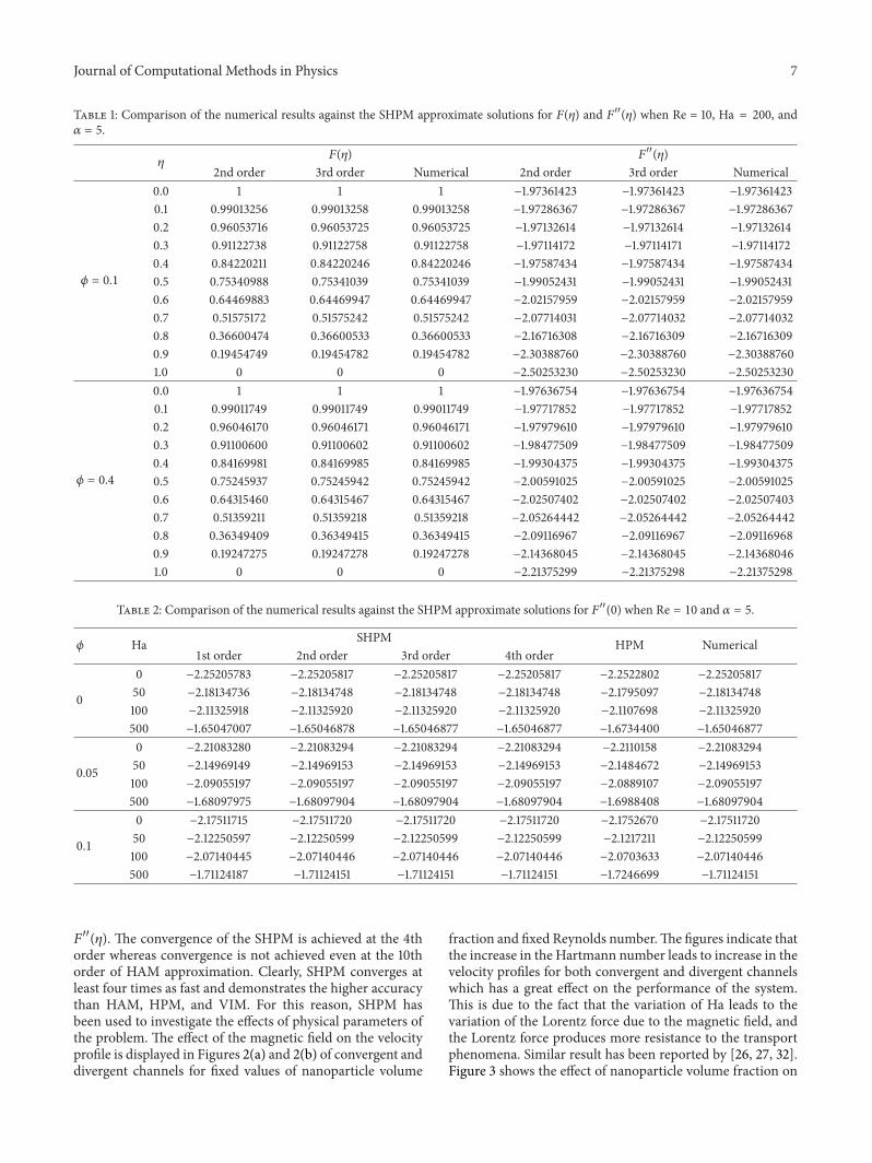