research article an integrated model for production and...

Research ArticleAn Integrated Model for Production andDistribution Planning of Perishable Products withInventory and Routing Considerations

S. M. Seyedhosseini and S. M. Ghoreyshi

Department of Industrial Engineering, Iran University of Science & Technology, P.O. Box 1684613114, Narmak, Tehran, Iran

Correspondence should be addressed to S. M. Ghoreyshi; [email protected]

Received 28 January 2014; Revised 22 April 2014; Accepted 25 April 2014; Published 12 May 2014

Academic Editor: Michael Freitag

Copyright © 2014 S. M. Seyedhosseini and S. M. Ghoreyshi.This is an open access article distributed under the Creative CommonsAttribution License, which permits unrestricted use, distribution, and reproduction in any medium, provided the original work isproperly cited.

In many conventional supply chains, production planning and distribution planning are treated separately. However, it is nowdemonstrated that they are mutually related problems that must be tackled in an integrated way. Hence, in this paper a newintegrated production and distribution planning model for perishable products is formulated. The proposed model considers asupply chain network consisting of a production facility and multiple distribution centers. The facility produces a single perishableproduct that is storable only for predetermined periods. A homogenous fleet of vehicles is responsible for delivering the productfrom facility to distribution centers. The decisions to be made are the production quantities, the distribution centers that mustbe visited, and the quantities to be delivered to them. The objective is to minimize the total cost, where the trip minimization isconsidered simultaneously. As the proposed formulation is computationally complex, a heuristic method is developed to tackle theproblem. In the developed method, the problem is divided into production submodel and distribution submodel. The productionsubmodel is solved using LINGO, and a particle swarm heuristic is developed to tackle distribution submodel. Efficiency of thealgorithm is proved through a number of randomly generated test problems.

1. Introduction

During the past decades, mangers have faced big globalchanges in the business environment as results of advancesin technology, globalization of markets, and new situationsin economy and politics. With the increase of the numberof world-class competitors, organizations have been underpressure to improve their interorganizational processes. Insuch situations, managers understood that such changes notonly are not enough in long term, but also they must enterin management of their supply, distribution, and after salescompanies. With such an approach, the terms “supply chain”and “supply chain management” were created [1].

A supply chain includes all facilities, works, and activitiesthat are engaged in production and delivering a product orservice from suppliers (and their suppliers) to customers(and their customers). It includes but not limited to planningand management of material requisition, manufacturing,warehousing, distribution, and after sales services.The supply

chain management should coordinate such activities so thatcustomers can have high quality products with minimumpossible cost [2].

In any supply chain, two main areas that are veryimportant to the managers are production and distributionplanning. Production planning tackles decision of how totransform raw materials into finished products respecting tomeet demands on time with minimum cost. Determininglot sizes, that is, calculating the quantity to be producecdfor each item at each time, is an important decision in tac-tical production planning. Considerations such as planninghorizon, number of levels, number of products, capacity orresource constraints, deterioration of items, demand type,setup structure, and inventory shortage may complicate thelot sizing problem [3]. For detailed information regardingclassifications and characteristics of lot sizing problem, see,for instance, Ben-Daya et al. [4], Robinson et al. [5], andBuschkuhl et al. [6].

Hindawi Publishing CorporationMathematical Problems in EngineeringVolume 2014, Article ID 475606, 10 pageshttp://dx.doi.org/10.1155/2014/475606

2 Mathematical Problems in Engineering

On the other hand, distribution planning tackles decisionof how to deliver the finished products to the customersrespecting to meet their demands on time with minimumcost. Routing problem is among one of themodel types in theliterature that are applied to the distribution planning. In suchproblems, distribution of a product(s) from a central locationto multiple geographically dispersed customers using defi-nite/indefinite number of capacitated vehicles is considered.The decisions to be made are (1) when to deliver to eachcustomer, (2) how much to deliver to each customer at eachtime, and (3) how to serve customers using the vehicles [7].

In a conventional supply chain, independentmanufactur-ers, wholesalers, and retailers were separate business entitiesseeking to maximize their own profits. However, it is nowdemonstrated that the production and distribution decisionsare mutually related problems that need to be dealt with inan integrated way. Integrated production and distributionplanning in the context of supply chain management hasbeen under attention of many researchers over the past fewyears.There might be two primary reasons behind this trend:(1) positive effect of integrated production and distributionplanning on profitability of supply chains and (2) positiveeffect of integrated production and distribution planningon reducing lead times and offering quicker responses tomarket changes [8]. In this paper, we focus on the integratedproduction and distribution planning of perishable products.The organization of this paper is as follows. In the nextsection, related literature is reviewed and then in Section 3the studied problem is thoroughly defined and formulated. Asthe proposedmodel is hard to solve specially in large problemsizes, a heuristic method is developed which is efficient inlight of both quality of the solutions and the running time.Finally, concluding remarks and future research remarks aregiven in Section 6.

2. Literature Review

An integrated production and distribution system oftenincludes facility(s) producing the product(s) and numberof distribution centers warehousing products. An integratedproduction and distribution planning problem is the prob-lem of simultaneously finding the decision variables fromdifferent functions that have traditionally been optimizedindependently. Some of these variables are as follows:

(i) quantity of product(s) produced in facility(s) at eachplanning period,

(ii) inventory amount of product(s) temporarily stored infacility(s) at the end of each planning period,

(iii) quantity of product(s) shipped from facility(s) todistribution centers in each planning period,

(iv) inventory of finished products stored in distributioncenters at the end of each planning period.

Due to the number of decision variables to be determined,the integrated production and distribution planning problemis so complex that optimal values are very hard to obtain.In addition, considerations such as complex structure of

the network, geographical span of the supply chain, andinvolvement of different entities with conflicting objectivescan further complicate the problem [9]. It is worthy to notethat integrated production and distribution planning prob-lems arise in environments where vendormanaged inventory(VMI) is implemented. In vendor managed inventory (VMI)environments, the supplier/manufacturer manages invento-ries at customers to ensure that they donot face any shortages.

The integrated production and distribution planningproblem has received a lot of attention among researchersparticularly in the recent years. Sarmiento and Nagi [10],Chen [11], and Fahimnia et al. [8] provided comprehensivereviews on the general subject. Below we mention somemore recent researches. Bard and Nananukul [12] formulatedan integrated lot sizing and inventory routing problem as amixed integer program with the objective of maximizing thenet.They developed a two-step procedure that first estimateddaily delivery quantities and then solved a vehicle routingproblem for each day of the planning horizon. Boudia andPrins [13] studied an NP-hard multiperiod production—distribution problem to minimize sum of three costs: pro-duction setups, inventories, and distribution. This problemthen was solved by a memetic algorithm with populationmanagement (MAPM). Bard and Nananukul [14] presenteda model that included a single production facility and a setof customers with time varying demand. They developed aprocedure centering on reactive tabu search for solving theproblem. Bilgen and Gunther [15] presented an integratedproduction scheduling and truck routing model for a supplychain of fruit juice. They considered different transportationmodes. Bard and Nananukul [16] investigated their previ-ously developed model aimed at minimizing costs. They alsodeveloped a hybrid methodology that combined exact andheuristic procedures within a branch-and-price framework.Bolduc et al. [17] proposed a tabu search heuristic for thesplit delivery vehicle routing problem with production anddemand calendars. Jolai et al. [18] considered a supply chainnetwork consisting of a manufacturer, with multiple plants,products, distribution centers, retailers, and customers. Theydeveloped a multiobjective linear programming model forintegrating production—distribution decisions. They alsoproposed three metaheuristics to tackle the problem. Toptalet al. [19] considered a joint production and transportationplanning problem where two vehicle types were available foroutbound shipments. They also presented formulations forthree different solution approaches. Nananukul [20] intro-duced an enhanced clustering model for the latter problem.An algorithm based on a reactive tabu search for solving theclustering problem was also proposed. Liu and Papageorgiou[21] addressed production, distribution, and capacity plan-ning of global supply chains considering cost, responsiveness,and customer service level simultaneously. They developeda multiobjective mixed-integer linear program (MILP) withtotal cost, total flow time, and total lost sales as key objectives.

Considering perishable products, production/inventoryand distribution decisions are often studied separately. Manyresearchers focused on extending economic productionquantity (EPQ) and economic order quantity (EOQ) modelsfor such products. The reader may refer to Nahimias [22],

Mathematical Problems in Engineering 3

Raafat [23], Goyal and Giri [24], and Bakker et al. [25] forcomprehensive reviews.

On the other hand, some researchers focused on extend-ing distribution planningmodels with concentration on vehi-cle routing problem for perishable products. Tarantilis andKiranoudis [26] proposed a fast and robust algorithm to findeffective delivery schedules for one of the biggest diary com-panies in Greece.They formulated the milk delivery problemas a heterogeneous fixed fleet vehicle routing problem (VRP).Chen andVairaktarakis [27] studied an integrated schedulingmodel of production and distribution operations in foodcatering service industries. In their model, a set of customerorders was first processed in a facility and then delivered tothe customers directly.The problemwas to find a joint sched-ule of production and distribution such that customer servicelevel and total distribution cost objectives were optimized.Hsu et al. [28] developed a stochastic VRPwith timewindowsformulation for delivery of perishable food products.The goalof their model was to find delivery paths, workloads, anddeparture times. Similarly, researches like Osvald and Stirn[29], Chen et al. [30], and Gong and Fu [31] applied VRPwith time windows to distribution planning of perishableproducts. Osvald and Stirn [29] formulated a vehicle routingproblemwith timewindows and time-dependent travel times(VRPTWTD) where the travel times between two locationsdepend on both the distance and on the time of the day.Theirmodel considered the impact of the perishability as part of theoverall distribution costs and a tabu search heuristic was usedto solve the problem. Chen et al. [30] proposed a nonlinearmathematical model for production scheduling and vehiclerouting with time windows for perishable food products.They assumed stochastic demands at retailers. Gong and Fu[31] proposed a multiobjective vehicle routing problem withtimewindowmodel that includes fixed vehicle cost, operationcost, shelf life loss, and default cost. They applied an antcolony optimizationwith ABC customer classification (ABC-ACO) to solve the problem.

To the best of our knowledge, no research has ever tack-led the integrated problem of production and distributionplanning of perishable products with inventory and routingconsiderations. Therefore, in this paper we deal with anintegratedmodel for production and distribution planning ofperishable products.

3. Problem Statement

In this section, the studied problem is defined with detailsand the proposed model is formulated. We are given asingle production facility that produces a single perishableproduct. The perishable product has a fixed lifetime that ismeasured by a number of planning periods that can be storedeither in the production facility or in distribution centers.The planning horizon is divided into 𝑇 equal discrete timeinterval that each one is a planning period. The productioncapacity in each planning period is limited to 𝑝max. If wehave production at the facility in planning period 𝑡, then aconsiderable setup cost 𝑓𝑝𝑐

𝑡(𝑡 = 1, . . . , 𝑇) is incurred. A

limited amount of inventory can be temporarily stored in

the production facility with unit holding cost of ℎ0. There

is a set of 𝑛 distribution centers geographically dispersedaround the production facility that the products are to bedelivered to them. Each distribution center 𝑖 (𝑖 = 1, 2, . . . , 𝑛)

has a nonnegative and deterministic demand 𝑑𝑖,𝑡in planning

period 𝑡 of the planning horizon that must be fully met; thatis, shortages are not allowed. A limited amount of inventorycan be stored in distribution center 𝑖 with unit holdingcost of ℎ

𝑖. A fleet of 𝐾 capacitated homogeneous vehicles is

responsible for shipping of the product from the facility tothe distribution centers. The company is not owner of fleetand incurred costs are calculated based of number of tripsvehicles make, not the distance they travel.Therefore, we aimto minimize the number of vehicles’ trips. In addition, twoother rules must be applied to deliveries; each vehicle canmake at most one delivery per planning period and eachdistribution center can be visited at most once per planningperiod.

Our objective is to construct a production-distributionplan by integrating production, inventory, and routing deci-sions that minimizes total costs while ensuring that alldemands are met and there is no shortage. The model mustdetermine, for each planning period, whether there mustbe production or not, the amount to be produced, thedistribution centers that must be visited, and the quantitiesto be delivered to them. Considering the setup cost, variableproduction cost, and inventory holding costs over the plan-ning horizon, the model must decide when to overproduceand when to hold items as inventory.

In standard models, the inventory levels are onlyrestricted by the physical storage capacities, while in ourmodel, the perishability dominates the physical storagecapacity. We defined an upper bound for inventory levels atproduction facility and distribution centers. Considering sl asthe shelf life of the perishable product, the inventory upperbound for production facility in planning period 𝑡 is equal tothe sum of all distribution centers’ demands in that periodand next sl planning periods. Similarly, the inventory upperbound for distribution center 𝑖 in planning period 𝑡 is equalto the sum of its demands in that period and next sl planningperiods.These upper bounds are ourmain contribution of theformulation.

In the development of the model, see Nomenclaturesection.

The formulated model is as follows.

Integrated Production and Distribution Model. Consider

Min ∑

𝑡

𝑓𝑝𝑐𝑡⋅ 𝑍𝑡+∑

𝑡

V𝑝𝑐𝑡⋅ 𝑃𝑡+∑

𝑡

ℎ0⋅ 𝐼0,𝑡+∑

𝑖,𝑡

ℎ𝑖⋅ 𝐼𝑖,𝑡

+∑

𝑘,𝑡

𝑓𝑡𝑐𝑘⋅ 𝑌𝑘,𝑡

(1)

𝐼0,𝑡= 𝐼0,𝑡−1

+ 𝑃𝑡−∑

𝑖

∑

𝑘

𝑊𝑖,𝑘,𝑡

∀𝑡 ∈ 𝑇 (2)


𝐼𝑖,𝑡= 𝐼𝑖,𝑡−1

+∑

𝑘

𝑊𝑖,𝑘,𝑡

− 𝑑𝑖,𝑡

∀𝑖 ∈ 𝑁, 𝑡 ∈ 𝑇 (3)

𝐼0,𝑡≤ 𝑢0,𝑡

∀𝑡 ∈ 𝑇 (4)

𝐼𝑖,𝑡≤ 𝑢𝑖,𝑡

∀𝑖 ∈ 𝑁, 𝑡 ∈ 𝑇 (5)

𝑃𝑡≤ 𝑝max ⋅ 𝑍𝑡 ∀𝑡 ∈ 𝑇 (6)

𝑊𝑖,𝑘,𝑡

≤ 𝑞 ⋅ 𝑋𝑖,𝑘,𝑡

∀𝑖 ∈ 𝑁, 𝑘 ∈ 𝐾, 𝑡 ∈ 𝑇 (7)

∑

𝑖

𝑊𝑖,𝑘,𝑡

≤ 𝑞 ∀𝑘 ∈ 𝐾, 𝑡 ∈ 𝑇 (8)

∑

𝑘

𝑋𝑖,𝑘,𝑡

≤ 1 ∀𝑖 ∈ 𝑁, 𝑡 ∈ 𝑇 (9)

∑

𝑖

𝑋𝑖,𝑘,𝑡

≤ 1 ∀𝑘 ∈ 𝐾, 𝑡 ∈ 𝑇 (10)

∑

𝑖

𝑋𝑖,𝑘,𝑡

≤ 𝑞 ⋅ 𝑌𝑘,𝑡

∀𝑘 ∈ 𝐾, 𝑡 ∈ 𝑇 (11)

𝑍𝑡, 𝑋𝑖,𝑘,𝑡

, 𝑌𝑘,𝑡∈ {0, 1} ∀𝑖 ∈ 𝑁, 𝑘 ∈ 𝐾, 𝑡 ∈ 𝑇 (12)

𝑃𝑡, 𝐼0,𝑡, 𝐼𝑖,𝑡,𝑊𝑖,𝑘,𝑡

≥ 0 ∀𝑖 ∈ 𝑁, 𝑘 ∈ 𝐾, 𝑡 ∈ 𝑇. (13)

In the above model, objective function (1) minimizes thesum of all costs. Note that the term ∑

𝑘,𝑡𝑓𝑡𝑐𝑘⋅ 𝑌𝑘,𝑡

aims atminimizing the total number of vehicles trips in planninghorizon. Constraints (2) are inventory balance equationsat production facility that relate its inventory levels to theproduction quantities and deliveries to distribution centers.Similarly, constraints (3) are inventory balance equations atdistribution centers. Constraints (4) and (5) guarantee thatinventory levels at production facility or distribution centersare never greater than the total demands in next sl followingperiods.These constraints guarantee that perishable productswill never be thrown away. Production quantities in plan-ning period 𝑡 are limited to the production capacity usingconstraints (6). Constraints (7) demonstrate that if there isa delivery to a distribution center in a planning period, thenthe pertaining binary variable must be 1. Vehicle capacity isrespected by constraints (8). Constraints (9) guarantee thateach distribution center is visited mostly once per planningperiod. Similarly, constraints (10) guarantee that each vehicleis used mostly once per planning period. Constraints (11)demonstrate number of vehicles’ trips during planning hori-zon. Finally, relations (12) and (13) present decision variablestypes.

The size of proposed model is determined largely byconstraints (7) and the number of binary variables 𝑋

𝑖,𝑘,𝑡,

which both grow at a rate proportional to𝑂(𝑁𝐾𝑇). A typicalproblem with 20 vehicles, 50 distribution centers, and a 10-day planning horizon contains roughly 12000 constraints,10000 binary variables, and 10000 continuous variables.Initial attempts to solve instances of this size with LINGO

commercial optimizer were not encouraging. This led todevelopment of a more efficient algorithm presented in thenext section.

4. Solution Method

In this section, a two-phase algorithm is presented to solvethe proposed model. We face two types of decision variablesin themodel, the variables pertaining to production decisions(𝑍𝑡, 𝑃𝑡, 𝐼0,𝑡), and the variables pertaining to distribution

decisions (𝑋𝑖,𝑘,𝑡

, 𝑌𝑘,𝑡,𝑊𝑖,𝑘,𝑡

, 𝐼𝑖,𝑡). A natural way to solve an

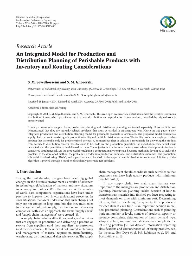
integrated model is to decompose the problem and considereach part dependently. In this way, we can separate theintegratedmodel into two dependent submodels, the produc-tion submodel and the distribution submodel. In proposedmethod, the production submodel is solved first and thepertaining variables are determined. Then, the results arefed back into the distribution submodel and the pertainingvariables are determined. In the next step, the productionsubmodel is solved again considering the previous step.The algorithm continues this iterative solve-feedback-solveprocedure until a stopping criterion is met. The details of theproposed method are given in Algorithm 1.

The algorithm consists of two phases, decompositionphase and integration phase. In the decomposition phase, thefirst iteration of the algorithm, the optimal lot sizes are foundconsidering the sum of distribution centers’ demands in eachplanning period as demand of that period. The productionsubmodel is demonstrated in relations (14) to (19). It is avariation of lot sizing model and it is easy to solve by anycommercial optimizer such as LINGO. In this submodel, thefollowing additional parameter is used.

Additional Parameters. 𝐷𝑡is the sum of distribution centers’

demands in planning period 𝑡(𝐷𝑡= ∑𝑖𝑑𝑖,𝑡; ∀𝑡 ∈ 𝑇).

Production Submodel. Consider

Min ∑

𝑡


𝑡


𝑡

ℎ0⋅ 𝐼0,𝑡 (14)

𝐼0,𝑡= 𝐼0,𝑡−1

+ 𝑃𝑡− 𝐷𝑡

∀𝑡 ∈ 𝑇 (15)


∀𝑡 ∈ 𝑇 (16)


𝑍𝑡∈ {0, 1} ∀𝑡 ∈ 𝑇 (18)

𝑃𝑡, 𝐼0,𝑡≥ ∀𝑡 ∈ 𝑇. (19)

Then, the algorithm proceeds with finding the quantityof products to be delivered to each distribution centerand the distribution centers that each vehicle must visit ineach planning period. This is done through the distributionsubmodel. Relations (20) to (30) demonstrate the distributionsubmodel. The production quantities (𝑃

𝑡) from production

submodel work as input parameter to this submodel.


! Decomposition phaseSolve production sub model using LINGOSolve distribution sub model using Particle Swarm HeuristicSave the solution as CURRENT SOLUTION and BEST SOLUTIONCalculate CURRENT COST and set BEST COST = CURRENT COST! End of decomposition phase! Integration phaseWhile the stopping criterion is not metUpdate ARTIFICIAL DEMANDRun Perturbation MechanismSolve production sub model using LINGO considering ARTIFICIAL SETUP COST andARTIFICIAL HOLDING COSTSolve distribution sub model using Particle Swarm HeuristicSave the solution as CURRENT SOLUTIONCalculate the CURRENT COSTIf (CURRENT COST < BEST COST)

Set BEST SOLUTION = CURRENT SOLUTIONSet BEST COST = CURRENT COST

End IfEnd While! End of integration phaseReturn BEST SOLUTION and BEST COST

Algorithm 1: Detailed steps of proposed method.

Distribution Submodel. Consider

Min ∑

𝑖,𝑡

ℎ𝑖⋅ 𝐼𝑖,𝑡+∑

𝑘,𝑡

𝑓𝑡𝑐𝑘⋅ 𝑌𝑘,𝑡 (20)

𝐼0,𝑡= 𝐼0,𝑡−1

+ 𝑃𝑡−∑

𝑖

∑

𝑘

𝑊𝑖,𝑘,𝑡

∀𝑡 ∈ 𝑇 (21)


+∑

𝑘

𝑊𝑖,𝑘,𝑡

− 𝑑𝑖,𝑡

∀𝑖 ∈ 𝑁, 𝑡 ∈ 𝑇 (22)


∀𝑖 ∈ 𝑁, 𝑡 ∈ 𝑇 (23)

𝑊𝑖,𝑘,𝑡

≤ 𝑞 ⋅ 𝑋𝑖,𝑘,𝑡

∀𝑖 ∈ 𝑁, 𝑘 ∈ 𝐾, 𝑡 ∈ 𝑇 (24)

∑

𝑖

𝑊𝑖,𝑘,𝑡

≤ 𝑞 ∀𝑘 ∈ 𝐾, 𝑡 ∈ 𝑇 (25)

∑

𝑘

𝑋𝑖,𝑘,𝑡

≤ 1 ∀𝑖 ∈ 𝑁, 𝑡 ∈ 𝑇 (26)

∑

𝑖

𝑋𝑖,𝑘,𝑡

≤ 1 ∀𝑘 ∈ 𝐾, 𝑡 ∈ 𝑇 (27)

∑

𝑖

𝑋𝑖,𝑘,𝑡

≤ 𝑞 ⋅ 𝑌𝑘,𝑡

∀𝑘 ∈ 𝐾 (28)

𝑋𝑖,𝑘,𝑡

, 𝑌𝑘,𝑡∈ {0, 1} ∀𝑖 ∈ 𝑁, 𝑘 ∈ 𝐾, 𝑡 ∈ 𝑇 (29)

𝐼0,𝑡, 𝐼𝑖,𝑡,𝑊𝑖,𝑘,𝑡

≥ 0 ∀𝑖 ∈ 𝑁, 𝑘 ∈ 𝐾, 𝑡 ∈ 𝑇. (30)

During initial test, we found that LINGO is not able tofind optimal or good quality solution for the above submodelin a reasonable time. Therefore, we used LINGO to obtain

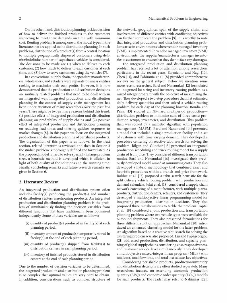
initial feasible solution and then a particle swarm basedheuristic to improve it.

Particle swarm optimization (PSO) simulates the socialbehavior of natural organisms such as bird flocking andfish schooling to find a place with enough food. Indeed, inthose swarms, a coordinated behavior using local movementsemergeswithout any central control. In PSO, a swarmconsistsof number of particles. Each particle is a candidate solutionto the problem. A particle has its own position and velocity.Optimization takes advantage of the cooperation betweenthe particles. The success of some particles will influence thebehavior of the others. Each particle successively adjusts itsposition according to the following two factors: the best posi-tion visited by itself and the best position visited by the wholeswarm [32]. Originally, PSO has been successfully designedfor continuous optimization problems in [33, 34]. However,Kennedy and Eberhart [35] firstly introduced discrete versionof PSO.

The details of proposed heuristic are given inAlgorithm 2.

In particle swarmheuristic, how to encode the problem toset of particles is of great importance. Consider the problemin which𝑁 distribution centers are to be served by𝐾 vehiclesin 𝑇 planning periods; we have to map a 2-dimensional arrayof (𝑁×𝐾, 𝑇) for each particle.The first dimension includes𝐾sections, where each section has𝑁 binary points.The seconddimension includes 𝑇 binary points. If a value is equal to1, it represents that the corresponding distribution center isserved by the relevant vehicle in relevant planning period.An example of encoding structure for problem with fivedistribution centers, two vehicles, and five planning periodsis given in Table 1.


Run LINGO to find an initial feasible solutionSet the initial feasible solution as Localbest Solution and Globalbest SolutionGenerate particles and set all equal to initial feasible solutionSet all the particles equal to initial feasible solutionWhile the stopping criterion is not met

For each particle𝑋, calculate 𝑉 = 𝑉 + 𝛼 ⋅ (𝑋𝑙𝑜𝑐𝑎𝑙𝑏𝑒𝑠𝑡

− 𝑋) + 𝛽 ⋅ (𝑋𝑔𝑙𝑜𝑏𝑎𝑙𝑏𝑒𝑠𝑡

− 𝑋).For each bit 𝑥𝑗 in particle𝑋, If (rand < Sigmoid(V𝑗)) then 𝑥𝑗 = 1, else 𝑥𝑗 = 0Check feasibility for each particle and repair the particleCalculate fitness function for each particleUpdate Localbest Solution and Globalbest Solution

End whileRun LINGO using Globalbest Solution to obtain real valued variables

Algorithm 2: Details of particle swarm heuristic.

Table 1: An example of encoding structure.

Served by vehicle 1 Served by vehicle 2DC-1 DC-2 DC-3 DC-4 DC-5 DC-1 DC-2 DC-3 DC-4 DC-5

Period 1 1 1 0 0 0 0 0 1 1 1Period 2 1 0 1 0 0 0 1 0 1 0Period 3 0 0 0 0 1 0 1 1 0 0Period 4 1 0 0 1 0 0 0 0 0 0Period 5 0 0 0 0 0 1 0 0 0 0

Based on the formulation, the following rules must berespected in each solution: (1) each distribution center mustbe served at most once per planning period, (2) each vehiclecan make at most one delivery per planning period, and(3) the perishability of the product must be respected; thatis, time between two consecutive delivery to a distributioncenter must be at most equal to the shelf life of the product.For instance, if the shelf life of the product is 2 days, a deliveryon Monday and another onThursday is not allowed, becauseit results in shortage. During the algorithm run, if any of theabove rules was violated, the solution becomes infeasible andmust be repaired. For rules 1 and 2, if the value of more thanone position in the corresponding positions in any particle is1, we randomly select one position and set its value to 1 andthe others to 0. For rule 3, consider that values correspondingto planning periods 𝑎 and 𝑏 are 1 in a particle. Without lossof generality, let us assume that 𝑎 < 𝑎 + sl < 𝑏. We set thecorresponding value to planning period 𝑏 = 0 and set thevalue corresponding to planning period 𝑎 + sl = 1.

During algorithm run, each particle must be measuredaccording to a fitness function. Becausewe aim atminimizingthe total number of vehicles trips, the term ∑

𝑖,𝑘,𝑡𝑓𝑡𝑐𝑘⋅ 𝑋𝑖,𝑘,𝑡

is used as fitness function. Finally, when the binary variables𝑋𝑖,𝑘,𝑡

and 𝑌𝑘,𝑡

are determined via above procedure, we usethem as input to distribution subproblem in LINGO to findreal variables.

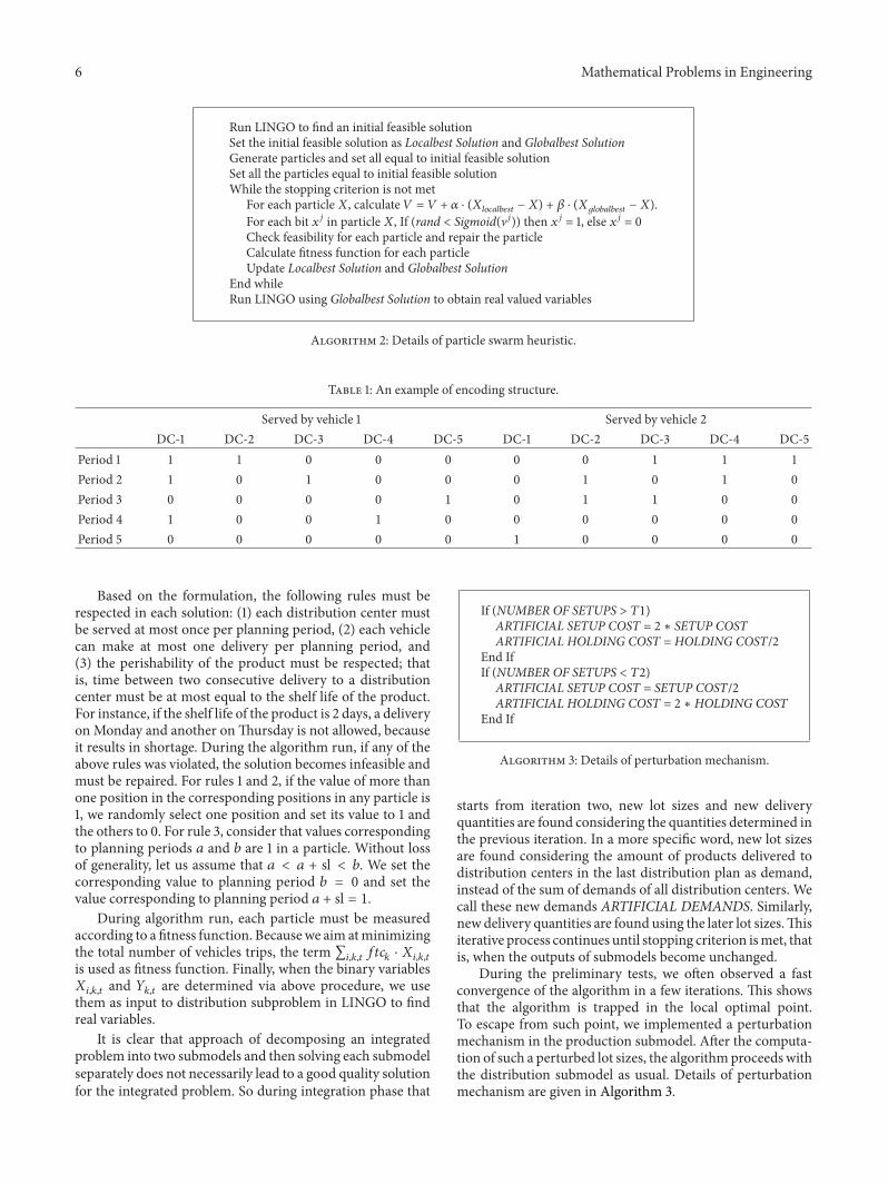
It is clear that approach of decomposing an integratedproblem into two submodels and then solving each submodelseparately does not necessarily lead to a good quality solutionfor the integrated problem. So during integration phase that

If (NUMBER OF SETUPS > 𝑇1)ARTIFICIAL SETUP COST = 2 ∗ SETUP COSTARTIFICIAL HOLDING COST = HOLDING COST/2

End IfIf (NUMBER OF SETUPS < 𝑇2)

ARTIFICIAL SETUP COST = SETUP COST/2ARTIFICIAL HOLDING COST = 2 ∗ HOLDING COST

End If

Algorithm 3: Details of perturbation mechanism.

starts from iteration two, new lot sizes and new deliveryquantities are found considering the quantities determined inthe previous iteration. In a more specific word, new lot sizesare found considering the amount of products delivered todistribution centers in the last distribution plan as demand,instead of the sum of demands of all distribution centers. Wecall these new demands ARTIFICIAL DEMANDS. Similarly,new delivery quantities are found using the later lot sizes.Thisiterative process continues until stopping criterion ismet, thatis, when the outputs of submodels become unchanged.

During the preliminary tests, we often observed a fastconvergence of the algorithm in a few iterations. This showsthat the algorithm is trapped in the local optimal point.To escape from such point, we implemented a perturbationmechanism in the production submodel. After the computa-tion of such a perturbed lot sizes, the algorithmproceeds withthe distribution submodel as usual. Details of perturbationmechanism are given in Algorithm 3.


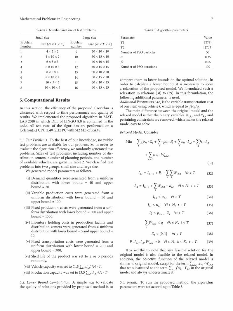
Table 2: Number and size of test problems.

Small size Large sizeProblemnumber Size (𝑁 × 𝑇 × 𝐾) Problem

number Size (𝑁 × 𝑇 × 𝐾)

1 4 × 5 × 2 9 30 × 10 × 10

2 4 × 10 × 2 10 30 × 15 × 10

3 6 × 5 × 3 11 40 × 10 × 15

4 6 × 10 × 3 12 40 × 15 × 15

5 8 × 5 × 4 13 50 × 10 × 20

6 8 × 10 × 4 14 50 × 15 × 20

7 10 × 5 × 5 15 60 × 10 × 25

8 10 × 10 × 5 16 60 × 15 × 25

5. Computational Results

In this section, the efficiency of the proposed algorithm isdiscussed with respect to time performance and quality ofresults. We implemented the proposed algorithm in MAT-LAB 2010 in which DLL of LINGO 8.0 is contained in thecode. All test runs of the algorithm are performed on aCeleron(R) CPU 2.40GHz PC with 512MB of RAM.

5.1. Test Problems. To the best of our knowledge, no publictest problems are available for our problem. So in order toevaluate the algorithm efficiency, we randomly generated testproblems. Sizes of test problems, including number of dis-tribution centers, number of planning periods, and numberof available vehicles, are given in Table 2. We classified testproblems into two groups, small size and large size.

We generated model parameters as follows.

(i) Demand quantities were generated from a uniformdistribution with lower bound = 10 and upperbound = 20.

(ii) Variable production costs were generated from auniform distribution with lower bound = 50 andupper bound = 100.

(iii) Fixed production costs were generated from a uni-form distribution with lower bound = 500 and upperbound = 1000.

(iv) Inventory holding costs in production facility anddistribution centers were generated from a uniformdistributionwith lower bound = 5 and upper bound =10.

(v) Fixed transportation costs were generated from auniform distribution with lower bound = 200 andupper bound = 300.

(vi) Shelf life of the product was set to 2 or 3 periodsrandomly.

(vii) Vehicle capacity was set to (1.5∑𝑖,𝑡𝑑𝑖,𝑡)/𝑁 ⋅ 𝑇.

(viii) Production capacity was set to (3.5∑𝑖,𝑡𝑑𝑖,𝑡)/𝑁 ⋅ 𝑇.

5.2. Lower Bound Computation. A simple way to validatethe quality of solutions provided by proposed method is to

Table 3: Algorithm parameters.

Parameter Value𝑇1 [𝑇/3]𝑇2 [2𝑇/3]Number of PSO particles 50𝛼 0.35𝛽 0.65Number of PSO iterations 100

compare them to lower bounds on the optimal solution. Inorder to calculate a lower bound, it is necessary to solvea relaxation of the proposed model. We formulated such arelaxation in relations (31) to (39). In this formulation, thefollowing additional parameter is used.Additional Parameters. V𝑡𝑐

𝑘is the variable transportation cost

of one item using vehicle 𝑘 which is equal to 𝑓𝑡𝑐𝑘/𝑞.

The main difference between the original model and therelaxed model is that the binary variables 𝑋

𝑖,𝑘,𝑡and 𝑌

𝑘,𝑡and

pertaining constraints are removed, which makes the relaxedmodel easy to solve.

Relaxed Model. Consider

Min ∑

𝑡


𝑡


𝑡

ℎ0⋅ 𝐼0,𝑡+∑

𝑖,𝑡

ℎ𝑖⋅ 𝐼𝑖,𝑡

+ ∑

𝑖,𝑘,𝑡

V𝑡𝑐𝑘⋅ 𝑊𝑖,𝑘,𝑡

(31)

𝐼0,𝑡= 𝐼0,𝑡−1

+ 𝑃𝑡−∑

𝑖

∑

𝑘

𝑊𝑖,𝑘,𝑡

∀𝑡 ∈ 𝑇 (32)


+∑

𝑘

𝑊𝑖,𝑘,𝑡

− 𝑑𝑖,𝑡

∀𝑖 ∈ 𝑁, 𝑡 ∈ 𝑇 (33)


∀𝑡 ∈ 𝑇 (34)


∀𝑖 ∈ 𝑁, 𝑡 ∈ 𝑇 (35)


∑

𝑖

𝑊𝑖,𝑘,𝑡

≤ 𝑞 ∀𝑘 ∈ 𝐾, 𝑡 ∈ 𝑇 (37)

𝑍𝑡∈ {0, 1} ∀𝑡 ∈ 𝑇 (38)

𝑃𝑡, 𝐼0,𝑡, 𝐼𝑖,𝑡,𝑊𝑖,𝑘,𝑡

≥ 0 ∀𝑖 ∈ 𝑁, 𝑘 ∈ 𝐾, 𝑡 ∈ 𝑇. (39)

It is worthy to note that any feasible solution for theoriginal model is also feasible to the relaxed model. Inaddition, the objective function of the relaxed model issimilar to original model, except for the term∑

𝑖,𝑘,𝑡V𝑡𝑐𝑘⋅𝑊𝑖,𝑘,𝑡

that we substituted to the term ∑𝑘,𝑡𝑓𝑡𝑐𝑘⋅ 𝑌𝑘,𝑡

in the originalmodel and always underestimate it.

5.3. Results. To run the proposed method, the algorithmparameters were set according to Table 3.


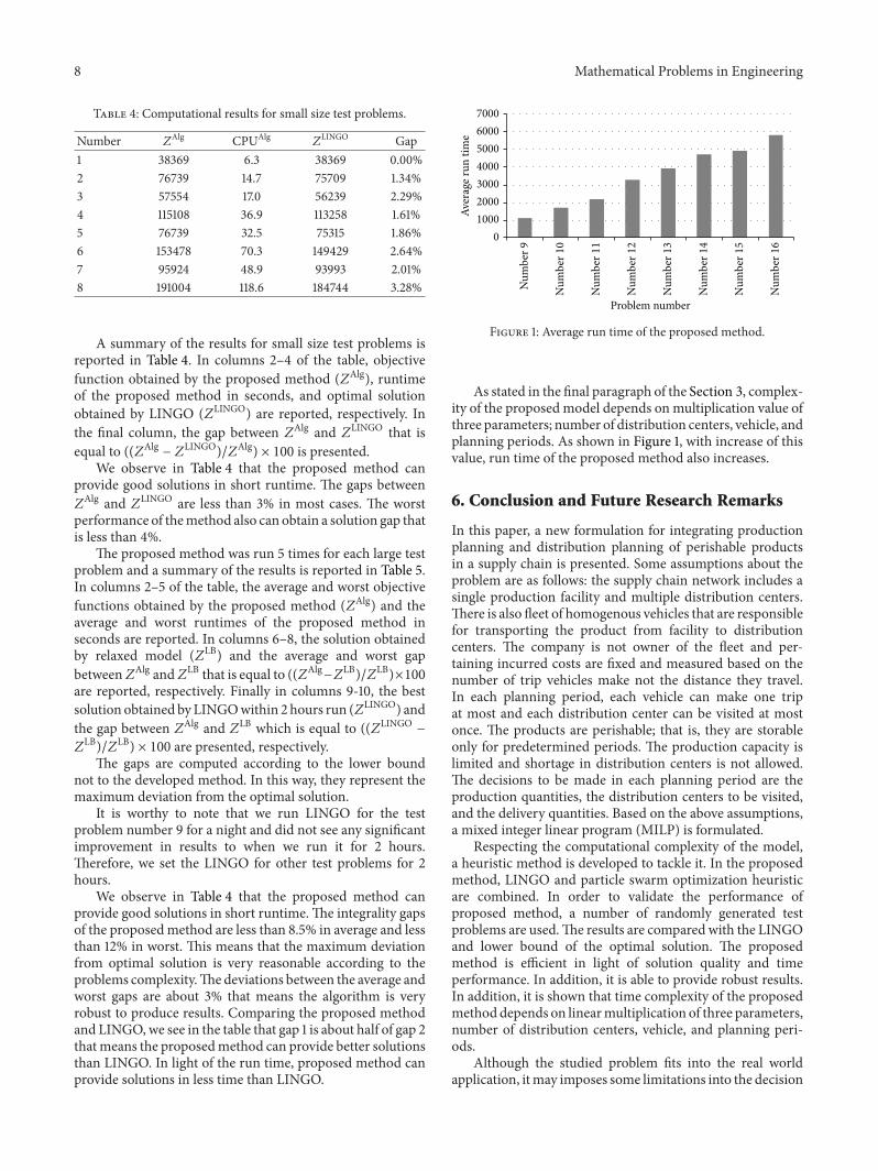
Table 4: Computational results for small size test problems.

Number 𝑍Alg CPUAlg

𝑍LINGO Gap

1 38369 6.3 38369 0.00%2 76739 14.7 75709 1.34%3 57554 17.0 56239 2.29%4 115108 36.9 113258 1.61%5 76739 32.5 75315 1.86%6 153478 70.3 149429 2.64%7 95924 48.9 93993 2.01%8 191004 118.6 184744 3.28%

A summary of the results for small size test problems isreported in Table 4. In columns 2–4 of the table, objectivefunction obtained by the proposed method (𝑍Alg

), runtimeof the proposed method in seconds, and optimal solutionobtained by LINGO (𝑍

LINGO) are reported, respectively. In

the final column, the gap between 𝑍Alg and 𝑍

LINGO that isequal to ((𝑍Alg

− 𝑍LINGO

)/𝑍Alg) × 100 is presented.

We observe in Table 4 that the proposed method canprovide good solutions in short runtime. The gaps between𝑍Alg and 𝑍

LINGO are less than 3% in most cases. The worstperformance of themethod also can obtain a solution gap thatis less than 4%.

The proposed method was run 5 times for each large testproblem and a summary of the results is reported in Table 5.In columns 2–5 of the table, the average and worst objectivefunctions obtained by the proposed method (𝑍Alg) and theaverage and worst runtimes of the proposed method inseconds are reported. In columns 6–8, the solution obtainedby relaxed model (𝑍LB) and the average and worst gapbetween𝑍Alg and𝑍LB that is equal to ((𝑍Alg

−𝑍LB)/𝑍

LB)×100

are reported, respectively. Finally in columns 9-10, the bestsolution obtained by LINGOwithin 2 hours run (𝑍LINGO) andthe gap between 𝑍Alg and 𝑍LB which is equal to ((𝑍LINGO

−

𝑍LB)/𝑍

LB) × 100 are presented, respectively.

The gaps are computed according to the lower boundnot to the developed method. In this way, they represent themaximum deviation from the optimal solution.

It is worthy to note that we run LINGO for the testproblem number 9 for a night and did not see any significantimprovement in results to when we run it for 2 hours.Therefore, we set the LINGO for other test problems for 2hours.

We observe in Table 4 that the proposed method canprovide good solutions in short runtime.The integrality gapsof the proposedmethod are less than 8.5% in average and lessthan 12% in worst. This means that the maximum deviationfrom optimal solution is very reasonable according to theproblems complexity.Thedeviations between the average andworst gaps are about 3% that means the algorithm is veryrobust to produce results. Comparing the proposed methodand LINGO, we see in the table that gap 1 is about half of gap 2thatmeans the proposedmethod can provide better solutionsthan LINGO. In light of the run time, proposed method canprovide solutions in less time than LINGO.

01000200030004000500060007000

Aver

age r

un ti

me

Num

ber9

Num

ber1

0

Num

ber1

1

Num

ber1

2

Num

ber1

3

Num

ber1

4

Num

ber1

5

Num

ber1

6

Problem number

Figure 1: Average run time of the proposed method.

As stated in the final paragraph of the Section 3, complex-ity of the proposed model depends onmultiplication value ofthree parameters; number of distribution centers, vehicle, andplanning periods. As shown in Figure 1, with increase of thisvalue, run time of the proposed method also increases.

6. Conclusion and Future Research Remarks

In this paper, a new formulation for integrating productionplanning and distribution planning of perishable productsin a supply chain is presented. Some assumptions about theproblem are as follows: the supply chain network includes asingle production facility and multiple distribution centers.There is also fleet of homogenous vehicles that are responsiblefor transporting the product from facility to distributioncenters. The company is not owner of the fleet and per-taining incurred costs are fixed and measured based on thenumber of trip vehicles make not the distance they travel.In each planning period, each vehicle can make one tripat most and each distribution center can be visited at mostonce. The products are perishable; that is, they are storableonly for predetermined periods. The production capacity islimited and shortage in distribution centers is not allowed.The decisions to be made in each planning period are theproduction quantities, the distribution centers to be visited,and the delivery quantities. Based on the above assumptions,a mixed integer linear program (MILP) is formulated.

Respecting the computational complexity of the model,a heuristic method is developed to tackle it. In the proposedmethod, LINGO and particle swarm optimization heuristicare combined. In order to validate the performance ofproposed method, a number of randomly generated testproblems are used.The results are compared with the LINGOand lower bound of the optimal solution. The proposedmethod is efficient in light of solution quality and timeperformance. In addition, it is able to provide robust results.In addition, it is shown that time complexity of the proposedmethod depends on linearmultiplication of three parameters,number of distribution centers, vehicle, and planning peri-ods.

Although the studied problem fits into the real worldapplication, itmay imposes some limitations into the decision


Table 5: Computational results (large size test problems).

Number 𝑍Alg CPUAlg

𝑍LB Gap 1

𝑍LINGO Gap 2

Avg. Worst Avg. Worst Avg. Worst9 556028 572704 1097 1141 526941 5.52% 8.68% 590796 12.12%10 834042 860841 1691 1773 769475 8.39% 11.87% 895742 16.41%11 741370 765830 2175 2244 692744 7.02% 10.55% 799822 15.46%12 1112056 1147772 3252 3374 1054671 5.44% 8.83% 1180939 11.97%13 926713 955584 3919 4039 863965 7.26% 10.60% 984028 13.90%14 1390069 1426843 4702 4924 1293635 7.45% 10.30% 1476745 14.15%15 1112056 1143883 4892 5088 1030104 7.96% 11.05% 1184692 15.01%16 1668083 1711109 5791 5965 1549744 7.64% 10.41% 1792531 15.67%

making. For example, the problem can be developed whenthe company owns the vehicle fleet and so the distance eachvehicle travels in each trip is important. In this situation, acustomized inventory routing model must be developed withrespect to problem definition. In addition, other real worldassumptions such as inventory transshipments between dis-tribution centers or split and delivery of the inventories can beadded to themodel. It should be noted that such assumptionscomplicate themodel, whichmay result inmore sophisticatedsolution methods.

Nomenclature

Indices

𝑡 = 1, 2, . . . , 𝑇: Set of planning periods𝑖 = 0, 1, . . . , 𝑁: Set of production facility and distribution

centers, where 0 corresponds toproduction facility

𝑘 = 1, 2, . . . , 𝐾: Set of vehicles.

Parameters

𝑑𝑖,𝑡: Demand of distribution center 𝑖 in

planning period 𝑡𝑓𝑝𝑐𝑡: Fixed production cost in planning period 𝑡

V𝑝𝑐𝑡: Variable production cost in planningperiod 𝑡

𝑝max: Production capacityℎ0: Inventory holding cost at production

facilityℎ𝑖: Inventory holding cost at distribution

center 𝑖sl: Shelf life of perishable products which is

measured in number of planning periodsthat the product can be stored

𝑢0,𝑡: Upper bound of inventory level at

production facility in planning period 𝑡,which is equal to ∑

𝑖∑𝑡≤𝜏≤𝑡+sl 𝑑𝑖,𝜏

𝑢𝑖,𝑡: Upper bound inventory level at

distribution center 𝑖 in planning period 𝑡,which is equal to ∑

𝑡≤𝜏≤𝑡+sl 𝑑𝑖,𝜏𝑞: Vehicle capacity𝑓𝑡𝑐𝑘: Fixed transportation cost of using vehicle𝑘.

Variables

𝑍𝑡: 1 if there is production on planning period

𝑡, 0 otherwise𝑃𝑡: Production quantity in planning period 𝑡

𝐼0,𝑡: Inventory level at production facility in

planning period 𝑡𝑋𝑖,𝑘,𝑡

: 1 if distribution 𝑖 is served by vehicle 𝑘 inplanning period 𝑡, 0 otherwise

𝑌𝑘,𝑡: 1 if vehicle 𝑘 is used in planning period 𝑡 to

serve distribution centers, 0 otherwise𝑊𝑖,𝑘,𝑡

: Amount delivered to distribution center 𝑖in planning period 𝑡 by vehicle 𝑘

𝐼𝑖,𝑡: Inventory level at distribution center 𝑖 in

planning period 𝑡.

Conflict of Interests

The authors declare that there is no conflict of interestsregarding the publication of this paper.

References

[1] D. Blanchard, Supply Chain Management Best Practices, JohnWiley & Sons, New York, NY, USA, 2010.

[2] S. Chopra and P. Meindl, Supply Chain Management. Strategy,Planning & Operation, Gabler, Wiesbaden, Germany, 2007.

[3] B. Karimi, S.M. T. FatemiGhomi, and J.M.Wilson, “The capac-itated lot sizing problem: a review of models and algorithms,”Omega, vol. 31, no. 5, pp. 365–378, 2003.

[4] M. Ben-Daya, M. Darwish, and K. Ertogral, “The joint eco-nomic lot sizing problem: review and extensions,” EuropeanJournal of Operational Research, vol. 185, no. 2, pp. 726–742,2008.

[5] P. Robinson, A. Narayanan, and F. Sahin, “Coordinated deter-ministic dynamic demand lot-sizing problem: a review ofmodels and algorithms,” Omega, vol. 37, no. 1, pp. 3–15, 2009.

[6] L. Buschkuhl, F. Sahling, S. Helber, and H. Tempelmeier,“Dynamic capacitated lot-sizing problems: a classification andreview of solution approaches,” OR Spectrum. QuantitativeApproaches in Management, vol. 32, no. 2, pp. 231–261, 2010.

[7] L. Bertazzi, M. Savelsbergh, and M. G. Speranza, “Inventoryrouting,” in The Vehicle Routing Problem: Latest Advances andNew Challenges, Springer, Berlin, Germany, 2008.

[8] B. Fahimnia, R. Zanjirani Farahani, R. Marian, and L. Luong,“A review and critique on integrated production-distribution


planning models and techniques,” Journal of ManufacturingSystems, vol. 32, no. 1, pp. 1–19, 2013.

[9] A. Pandey, M. Masin, and V. Prabhu, “Adaptive logistic con-troller for integrated design of distributed supply chains,”Journal of Manufacturing Systems, vol. 26, no. 2, pp. 108–115,2007.

[10] A.M. Sarmiento and R. Nagi, “A review of integrated analysis ofproduction-distribution systems,” IIE Transactions, vol. 31, no.11, pp. 1061–1074, 1999.

[11] Z.-L. Chen, “Integrated production and outbound distributionscheduling: review and extensions,” Operations Research, vol.58, no. 1, pp. 130–148, 2010.

[12] J. F. Bard and N. Nananukul, “Heuristics for a multiperiodinventory routing problem with production decisions,” Com-puters and Industrial Engineering, vol. 57, no. 3, pp. 713–723,2009.

[13] M. Boudia and C. Prins, “A memetic algorithm with dynamicpopulation management for an integrated production-distribution problem,” European Journal of OperationalResearch, vol. 195, no. 3, pp. 703–715, 2009.

[14] J. F. Bard and N. Nananukul, “The integrated production-inventory-distribution-routing problem,” Journal of Scheduling,vol. 12, no. 3, pp. 257–280, 2009.

[15] B. Bilgen and H.-O. Gunther, “Integrated production anddistribution planning in the fastmoving consumer goods indus-try: a block planning application,” OR Spectrum. QuantitativeApproaches in Management, vol. 32, no. 4, pp. 927–955, 2010.

[16] J. F. Bard and N. Nananukul, “A branch-and-price algorithmfor an integrated production and inventory routing problem,”Computers & Operations Research, vol. 37, no. 12, pp. 2202–2217,2010.

[17] M.-C. Bolduc, G. Laporte, J. Renaud, and F. F. Boctor, “A tabusearch heuristic for the split delivery vehicle routing problemwith production and demand calendars,” European Journal ofOperational Research, vol. 202, no. 1, pp. 122–130, 2010.

[18] F. Jolai, J. Razmi, and N. K. M. Rostami, “A fuzzy goal pro-gramming and meta heuristic algorithms for solving integratedproduction: distribution planning problem,” Central EuropeanJournal of Operations Research, vol. 19, no. 4, pp. 547–569, 2011.

[19] A. Toptal, U. Koc, and I. Sabuncuoglu, “A joint production andtransportation planning problem with heterogeneous vehicles,”Journal of the Operational Research Society, vol. 65, no. 1, pp.180–196, 2013.

[20] N.Nananukul, “Clusteringmodel and algorithm for productioninventory and distribution problem,” Applied MathematicalModelling, vol. 37, no. 24, pp. 9846–9857, 2013.

[21] S. Liu and L. G. Papageorgiou, “Multi objective optimisation ofproduction, distribution and capacity planning of global supplychains in the process industry,” Omega, vol. 41, no. 2, pp. 369–382, 2013.

[22] S. Nahmias, “Perishable inventory theory: a review,”OperationsResearch, vol. 30, no. 4, pp. 680–708, 1982.

[23] F. Raafat, “Survey of literature on continuously deterioratinginventory models,” Journal of the Operational Research Society,vol. 42, no. 1, pp. 27–37, 1991.

[24] S. K. Goyal and B. C. Giri, “Recent trends in modelingof deteriorating inventory,” European Journal of OperationalResearch, vol. 134, no. 1, pp. 1–16, 2001.

[25] M. Bakker, J. Riezebos, and R. H. Teunter, “Review of inventorysystems with deterioration since 2001,” European Journal ofOperational Research, vol. 221, no. 2, pp. 275–284, 2012.

[26] C. D. Tarantilis and C. T. Kiranoudis, “A meta-heuristic algo-rithm for the efficient distribution of perishable foods,” Journalof Food Engineering, vol. 50, no. 1, pp. 1–9, 2001.

[27] Z.-L. Chen and G. L. Vairaktarakis, “Integrated scheduling ofproduction and distribution operations,” Management Science,vol. 51, no. 4, pp. 614–628, 2005.

[28] C.-I. Hsu, S.-F. Hung, and H.-C. Li, “Vehicle routing problemwith time-windows for perishable food delivery,” Journal ofFood Engineering, vol. 80, no. 2, pp. 465–475, 2007.

[29] A. Osvald and L. Z. Stirn, “A vehicle routing algorithm for thedistribution of fresh vegetables and similar perishable food,”Journal of Food Engineering, vol. 85, no. 2, pp. 285–295, 2008.

[30] H.-K. Chen, C.-F. Hsueh, and M.-S. Chang, “Productionscheduling and vehicle routing with time windows for perish-able food products,” Computers & Operations Research, vol. 36,no. 7, pp. 2311–2319, 2009.

[31] W. Gong and Z. Fu, “ABC-ACO for perishable food vehiclerouting problem with time windows,” in Proceedings of theInternational Conference on Computational and InformationSciences (ICCIS ’10), pp. 1261–1264, December 2010.

[32] E.G. Talbi,Metaheuristics: FromDesign to Implementation, JohnWiley & Sons, New York, NY, USA, 2009.

[33] R. Eberhart and J. Kennedy, “New optimizer using particleswarm theory,” in Proceedings of the 6th International Sympo-sium onMicroMachine and Human Science, pp. 39–43, October1995.

[34] J. Kennedy and R. Eberhart, “A discrete binary version ofthe particle swarm algorithm,” in Proceeding of the IEEEInternational Conference on Systems, Man, and Cybernetics,Computational Cybernetics and Simulation, vol. 5, pp. 4104–4108, Orlando, Fla, USA, October 1997.

[35] J. Kennedy and R. Eberhart, “Particle swarm optimization,”in Proceeding of the IEEE International Conference on NeuralNetwork, pp. 1942–1948, December 1995.

Submit your manuscripts athttp://www.hindawi.com

Hindawi Publishing Corporationhttp://www.hindawi.com Volume 2014

MathematicsJournal of


Mathematical Problems in Engineering

Hindawi Publishing Corporationhttp://www.hindawi.com

Differential EquationsInternational Journal of

Volume 2014

Applied MathematicsJournal of


Probability and StatisticsHindawi Publishing Corporationhttp://www.hindawi.com Volume 2014

Journal of


Mathematical PhysicsAdvances in

Complex AnalysisJournal of


OptimizationJournal of


CombinatoricsHindawi Publishing Corporationhttp://www.hindawi.com Volume 2014

International Journal of


Operations ResearchAdvances in

Journal of


Function Spaces

Abstract and Applied AnalysisHindawi Publishing Corporationhttp://www.hindawi.com Volume 2014

International Journal of Mathematics and Mathematical Sciences


The Scientific World JournalHindawi Publishing Corporation http://www.hindawi.com Volume 2014


Algebra

Discrete Dynamics in Nature and Society



Decision SciencesAdvances in

Discrete MathematicsJournal of

Hindawi Publishing Corporationhttp://www.hindawi.com

Volume 2014 Hindawi Publishing Corporationhttp://www.hindawi.com Volume 2014

Stochastic AnalysisInternational Journal of

research article an integrated model for production and...

Documents