research article chebyshev-fourier spectral methods for
TRANSCRIPT

Research ArticleChebyshev-Fourier Spectral Methods for Nonperiodic BoundaryValue Problems
Bojan Orel1 and Andrej Perne2
1 Faculty of Computer and Information Science University of Ljubljana Trzaska Cesta 25 1000 Ljubljana Slovenia2 Faculty of Electrical Engineering University of Ljubljana Trzaska Cesta 25 1000 Ljubljana Slovenia
Correspondence should be addressed to Andrej Perne andrejpernefeuni-ljsi
Received 15 January 2014 Revised 9 May 2014 Accepted 13 May 2014 Published 1 June 2014
Academic Editor Miroslaw Lachowicz
Copyright copy 2014 B Orel and A PerneThis is an open access article distributed under the Creative CommonsAttribution Licensewhich permits unrestricted use distribution and reproduction in any medium provided the original work is properly cited
A new class of spectral methods for solving two-point boundary value problems for linear ordinary differential equations ispresented in the paper Although these methods are based on trigonometric functions they can be used for solving periodic aswell as nonperiodic problems Instead of using basis functions periodic on a given interval [minus1 1] we use functions periodic on awider intervalThe numerical solution of the given problem is sought in terms of the half-range Chebyshev-Fourier (HCF) series areorganization of the classical Fourier series using half-range Chebyshev polynomials of the first and second kind which were firstintroduced by Huybrechs (2010) and further analyzed by Orel and Perne (2012) The numerical solution is constructed as a HCFseries via differentiation andmultiplicationmatricesMoreover the construction of themethod error analysis convergence resultsand some numerical examples are presented in the paper The decay of the maximal absolute error according to the truncationnumber119873 for the new class of Chebyshev-Fourier-collocation (CFC)methods is compared to the decay of the error for the standardclass of Chebyshev-collocation (CC) methods
1 Introduction and Formulation
A standard problem in approximation theory is to computethe coefficients of a Fourier series to approximate smooth andperiodic functions This can be efficiently done by using theFFTwhich is a stable andwell-understoodmethod that yieldsspectral convergence Things look very different when deal-ing with nonperiodic or nonsmooth functions This is due tothe so called Gibbs phenomenon which causes oscillationsnear the points of discontinuity andor near the boundary aswell as slow decay of Fourier coefficients There are severalpossibilities to overcome these difficulties and successfullydeal with such functions Some of them were analyzed byGottlieb and Shu in [1] and by Tadmor in [2] One possibilityis to use some periodizing transformation and compute theFourier series of the transformed function There is a widelyused transformation which yields Chebyshev polynomials ofthe first kind Much about this can be found in the literatureby Boyd in [3] by Fornberg and Sloan in [4] or by Trefethenin [5]These polynomials are arranged as a Chebyshev series
Another approach was recently presented by Huybrechsin [6] where he analyzed the problem which was stated byBoyd in [7] and by Bruno et al in [8]
Problem 1 For 119879 gt 1 let 119866119899be the space of 2119879-periodic
functions of the form
119892 isin 119866119899 119892 (119909) =
1198860
2+
119899
sum119896=1
(119886119896cos 120587119896119909
119879+ 119887119896sin 120587119896119909
119879) (1)
The Fourier extension of 119891 isin 1198712
(minus1 1) defined on theinterval [minus1 1] to the interval [minus119879 119879] is the solution to theoptimization problem
119892119899= argmin
119892isin119866119899
1003817100381710038171003817119891 minus 11989210038171003817100381710038171198712 (2)
In his paper Huybrechs considered a square-integrablefunction 119891 isin 119871
2
(minus1 1) that is not necessarily smooth orperiodic The idea to obtain a spectrally accurate Fourierseries is to extend the given function 119891 to a function 119892 that
Hindawi Publishing CorporationJournal of Applied MathematicsVolume 2014 Article ID 572694 10 pageshttpdxdoiorg1011552014572694
2 Journal of Applied Mathematics
is periodic on a wider interval [minus119879 119879] 119879 gt 1 The Fourierseries of the constructed function is obviously point-wiseconvergent to 119891 on the interval [minus1 1]
Huybrechs analyzed this problem for the choice 119879 =
2 and developed three numerical methods for solving itBesides proving the existence and uniqueness of the solutionhe characterized the solution with two nonclassical familiesof orthogonal polynomials related to Chebyshev polynomialsof the first and second kind the half-range Chebyshevpolynomials of the first and second kind The second andthird methods are based on projection and collocationThe convergence is in most cases exponential rather thansuperalgebraic
The half-range Chebyshev polynomials of the first andsecond kind and the corresponding half-range Chebyshev-Fourier (HCF) series were further explored by Orel andPerne in [9] The authors presented an efficient method forthe construction of these polynomials using the modifiedChebyshev algorithm for the computation of the recursioncoefficients via the three-term recurrence relation formulaMoreover the authors developed some necessary tools for theconstruction of spectral methods using these polynomials
In this paper instead of approximation problems likeProblem 1 which was successfully solved by Huybrechs in[6] we are interested in solving BVPs in ODEs via spectralmethods that is solving problems as defined below
Problem 2 Find the numerical solution of a linear two-pointboundary value problem of the form
L119910 (119909) = 119891 (119909) 119909 isin [minus1 1] (3)
with boundary conditions
B119910 (119909) = 0 119909 isin minus1 1 (4)
whereL is a linear differential operator
L = 120572 (119909)1198892
1198891199092+ 120573 (119909)
119889
119889119909+ 120574 (119909) 119868 (5)
119868 is the identity operator and B is a set of linear boundarydifferential operators
There are several different classes of numerical methodsto solve boundary value problems In the company of suchmethods as finite differences (FDM) and finite elements(FEM) we are interested in spectral methods (SM) It is wellknown that spectral methods approximate the solution ina finite dimensional subspace of a Hilbert space The basisfunctions used are defined globally (on the whole interval)On the contrary the basis functions for finite elementmethods are defined locally (only on a small interval)
Different approaches are used if the underlying problemis periodic or nonperiodic In the case of periodic problemsthe natural basis functions are trigonometric functions Inother words the solution is approximated with a truncatedFourier series Equidistant mesh points are used to discretizethe interval on which the problem is defined In the caseof nonperiodic problems orthogonal polynomials are used
especially the Chebyshev polynomials of the first kind Inthis case the solution is approximated with a truncatedChebyshev series There are two types of Chebyshev meshpoints Chebyshev points of the second kind where theChebyshev polynomials of the first kind reach their extremevalues are generally used in spectral methods to discretizethe underlying interval Chebyshev points of the first kindare the zeros of the Chebyshev polynomials of the firstkind Usually Chebyshev points in nonperiodic problemsoutweigh equidistant points because they are denser nearthe boundary of the interval Besides such a distribution ofpoints overwhelms problems caused by Gibbs andor Rungephenomenon There are different types of spectral methodsdepending on the method used for computing the expansioncoefficients for example Galerkin method Tau methodor collocation Spectral methods based on collocation areusually called pseudospectral methods Classical referenceson spectral methods include textbooks by Boyd [3] Canutoet al [10] Fornberg [11] Gottlieb and Orszag [12] andTrefethen [5] and more recent ones are Canuto et al [13] andShen et al [14]
There were several attempts to solve nonperiodic prob-lems using a trigonometric basis Adcock in [15 16]solved the problem with modified Fourier series usingGalerkin method to compute expansion coefficients Huy-brechs in [6] proposed a new set of trigonometric functionswhich includes sines and cosines as well as half-sines andhalf-cosines
Our intention is to provide a new class of spectralmethods using approaches described in [6 9] combinedwith collocation to compute expansion coefficients Thisapproach yields pseudospectral method for solving nonperi-odic problems with tools used for solving periodic problemsWe focus on Dirichlet boundary conditions although it isnot difficult to extend this approach to Neumann or mixedboundary conditions The generalization to higher orderlinear boundary problems is also possible The restriction tothe interval [minus1 1] is only a matter of simplification since itis well known how to map an arbitrary interval [119886 119887] to theunit interval
The paper is organized as follows In Section 2 we definethe form of the exact solution to the discrete problem byintroducing the set of basis functions proposed byHuybrechsin [6] and two nonclassical families of orthogonal polyno-mials In Section 3 follows the developement of a spectralmethod for the solution of the boundary value problembased on a pseudospectral (collocation) approach Erroranalysis and convergence results based on error analysisapproach in [13 14] are addressed in Section 4 Finally wepresent some numerical examples in Section 5 Section 6concludes the paper
2 Approximation with Half-RangeChebyshev Polynomials
Let us first review the exact solution of the discrete Problem 1using the half-range Chebyshev polynomials The idea isto extend a nonperiodic function on the interval [minus1 1] toan interval [minus119879 119879] on which the given function is periodic
Journal of Applied Mathematics 3
and to use the set of trigonometric functions proposed byHuybrechs in [6] He analyzed the extension for 119879 = 2 andproposed to use the set of basis functions
119863119899= 119862119899cup 119878119899 (6)
where
119862119899=
1
radic2 cup cos 120587119896119909
2
119899
119896=1
119878119899= sin 120587119896119909
2
119899
119896=1
(7)
Note that the set 119862119899consists of even and the set 119878
119899of odd
functions The function space is the span of119863119899
Huybrechs showed that 119863infin
is not a basis of 1198712(minus1 1)but a tight frame with frame bound 2 that is the frameobeys a generalized Parsevalrsquos identity and that the set 119863
infin
consists of all eigenfunctions of the Laplace operator on[minus1 1] subject to either homogeneous Dirichlet or Neumannboundary conditionsThat is due to the fact that the functionsin 119863infin
are linearly dependent On the contrary the set 119863119899is
a basis for a finite dimensional subspace of 1198712(minus1 1) for anyfinite 119899 All the functions in119863
119899are linearly independent
It makes perfect sense to look for an orthonormal basison the interval [minus1 1] Since the even functions in 119862
119899
and the odd functions in 119878119899are mutually orthogonal the
orthonormalization problem divides into two problems Letus define two spaces denoted by
C119899= span 119862
119899 S
119899= span 119878
119899 (8)
The following two theorems are stated and proved by Huy-brechs in [6]
Theorem 3 Let 119879ℎ119896(119910) be the unique normalized sequence of
orthogonal polynomials satisfying
4
120587int1
0
119879ℎ
119896(119910) 119910ℓ
radic1 minus 1199102119889119910 = 120575
119896ℓ ℓ = 0 119896 minus 1 (9)
Then the set 119879ℎ119896(cos(1205871199092))119899
119896=0is an orthonormal basis forC
119899
on [minus1 1]
Theorem 4 Let 119880ℎ119896(119910) be the unique normalized sequence of
orthogonal polynomials satisfying
4
120587int1
0
119880ℎ
119896(119910) 119910ℓradic1 minus 1199102119889119910 = 120575
119896ℓ ℓ = 0 119896 minus 1 (10)
Then the set 119880ℎ119896(cos(1205871199092)) sin(1205871199092)119899minus1
119896=0is an orthonormal
basis for S119899on [minus1 1]
The polynomials 119879ℎ119899(119909) and 119880ℎ
119899(119909) are called half-range
Chebyshev polynomials of the first and second kind respec-tivelyThey have the same weight functions as the Chebyshevpolynomials of the first and second kind but are orthogonalon the interval [0 1] rather than on the interval [minus1 1] Theorthogonal polynomials are guaranteed to exist because theweight functions are positive and integrable The construc-tion and additional properties of these polynomials were
studied by Orel and Perne in [9] An arbitrary function 119891 isin
1198712
(minus1 1) can be then expanded as a half-range Chebyshev-Fourier series
119891 (119909) =
infin
sum119896=0
119886119896119879ℎ
119896(cos 120587119909
2) +
infin
sum119896=0
119887119896119880ℎ
119896(cos 120587119909
2) sin 120587119909
2
(11)
Huybrechs in [6] proved the existence and uniquenessof the exact solution to Problem 1 as a truncated half-rangeChebyshev-Fourier (HCF) series
Theorem5 For a given119891 isin 1198712(minus1 1) the solution to Problem1 is
119892119899(119909) =
119899
sum119896=0
119886119896119879ℎ
119896(cos 120587119909
2) +
119899minus1
sum119896=0
119887119896119880ℎ
119896(cos 120587119909
2) sin 120587119909
2
(12)
where
119886119896= int1
minus1
119891 (119909) 119879ℎ
119896(cos 120587119909
2) 119889119909
119887119896= int1
minus1
119891 (119909)119880ℎ
119896(cos 120587119909
2) sin 120587119909
2119889119909
(13)
Convergence of the HCF series (11) was extensivelystudied by Huybrechs in [6] where the following theoremand its corollary were stated and proved
Theorem 6 Let 119891(119910) = 119891(119909) where 119909 = (2120587) cosminus1119910be analytic in the region bounded by an ellipse with majorsemiaxis length 119877 and with foci 0 and 1 The correspondingdomain of analyticity of 119891 is denoted by 119863(119877) If 119891 is analyticin the domain 119863(119877) with 119877 gt 12 then the solution 119892
119899to the
Problem 1 satisfies1003817100381710038171003817119891 minus 119892119899
1003817100381710038171003817 sim 120588minus119899
(14)
with
120588 = min (3 + 2radic2 2119877 + radic41198772 minus 1) (15)
unless 119891 is analytic and periodic on [minus2 2]
Corollary 7 Under the conditions of Theorem 6 the coeffi-cients 119886
119896and 119887
119896of 119892119899in the form of (12) and (13) satisfy
119886119896 119887119896sim 120588minus119899
3 Construction of Chebyshev-Fourier-Collocation Methods
In this section we construct and analyze a new class ofspectral methods for the solution of Problem 2 which we willthen call Chebyshev-Fourier-collocation (CFC) methodsThe numerical solution is sought as a half-range Chebyshev-Fourier series defined in (12) The series is expanded interms of trigonometric functions and rearranged in termsof half-range Chebyshev polynomials defined in Theorems 3
4 Journal of Applied Mathematics
and 4 Collocation is used for the computation of expansioncoefficients defined in (13) Let us turn back to Problem 2 andrewrite it as a two-point boundary value problem (3) withDirichlet boundary conditions (4)
120572 (119909)1198892
119910
1198891199092+ 120573 (119909)
119889119910
119889119909+ 120574 (119909) 119910 = 119891 (119909) 119909 isin [minus1 1]
119910 (minus1) = 119860 119910 (1) = 119861
(16)
The numerical solution of the above problem is sought as atruncated HCF series introduced inTheorem 5
119910 (119909) asymp 119910119873(119909) =
119873
sum119896=0
119886119896119879ℎ
119896(cos 120587119909
2)
+
119873minus1
sum119896=0
119887119896119880ℎ
119896(cos 120587119909
2) sin 120587119909
2
(17)
In other words we seek for coefficients 119886119896and 119887119896 so that the
numerical solution (17) is as good as possible Here119873 is thetruncation number and for a given value of119873 we use 2119873 + 1
orthogonal polynomials 119873 + 1 half-range Chebyshev poly-nomials of the first and119873 half-range Chebyshev polynomialsof the second kind
We commence by dividing the interval [minus1 1]with 2119873+1collocation points the Chebyshev points of the second kindinto 2119873 subintervals
minus1 = 1199090lt 1199091lt sdot sdot sdot lt 119909
2119873= 1 (18)
where
119909119894= minus cos( 120587119894
2119873) 119894 = 0 1 2119873 (19)
Besides we compute the first derivative of the truncatedseries (17) where 1198861015840
119896and 1198871015840119896denote the coefficients of the first
derivative of the truncated HCF series
119889119910119873
119889119909(119909) =
119873
sum119896=0
1198861015840
119896119879ℎ
119896(cos 120587119909
2)
+
119873minus1
sum119896=0
1198871015840
119896119880ℎ
119896(cos 120587119909
2) sin 120587119909
2
(20)
We obtain a similar form (20) for the first derivative as forthe approximation of the solution (17)The coefficients 1198861015840
119896and
1198871015840
119896are linearly dependent on the coefficients 119886
119896and 119887119896and are
computed via the differentiation matrix119863
u1015840 = 119863u (21)
where u = (1198860 119886
119873 1198870 119887
119873minus1)119879 and u1015840 = (119886
1015840
0 119886
1015840
119873
1198871015840
0 119887
1015840
119873minus1)119879 Since the coefficients 1198861015840
119895depend only on 119887
119896and
1198871015840
119895only on 119886
119896 the differentiation matrix119863 isin R(2119873+1)times(2119873+1) is
block-antidiagonal
119863 =120587
2[0 1198671
11986720] (22)
where 1198671isin R(119873+1)times119873 and 119867
2isin R119873times(119873+1) This matrix was
constructed and studied in detail by Orel and Perne in [9]Furthermore we proceed by computing the second derivativeto obtain a similar representation
1198892
119910119873
1198891199092(119909) =
119873
sum119896=0
11988610158401015840
119896119879ℎ
119896(cos 120587119909
2)
+
119873minus1
sum119896=0
11988710158401015840
119896119880ℎ
119896(cos 120587119909
2) sin 120587119909
2
(23)
where the coefficients of the second derivative of the trun-cated series are denoted by 11988610158401015840
119896and 11988710158401015840119896 Again we compute
these coefficients using differentiation matrix119863
u10158401015840 = 1198632u (24)
where u10158401015840 = (119886101584010158400 119886
10158401015840
119873 11988710158401015840
0 119887
10158401015840
119873minus1)119879
Solving BVPs via collocation assumes that the numericalsolution of the BVP exactly solves the BVP in the interiorcollocation points (19) 119909
119894 119894 = 1 2 2119873minus1 After inserting
the truncated series (17) (20) and (23) into the differentialequation (3) we obtain a system of linear equations
120572 (119909119894)1198892
119910119873
1198891199092(119909119894) + 120573 (119909
119894)119889119910119873
119889119909(119909119894) + 120574 (119909
119894) 119910119873(119909119894)
= 119891 (119909119894) 119894 = 1 2 2119873 minus 1
(25)
Besides we have two additional equations originating inboundary value conditions
119873
sum119896=0
119886119896119879ℎ
119896(0) minus
119873minus1
sum119896=0
119887119896119880ℎ
119896(0) = 119860
119873
sum119896=0
119886119896119879ℎ
119896(0) +
119873minus1
sum119896=0
119887119896119880ℎ
119896(0) = 119861
(26)
Let us denote by 119862 isin R(2119873+1)times(2119873+1) the collocationmatrix The entries of this matrix are the values of the basisfunctions computed in the collocation points (19) If the setof all basis functions is denoted by 120601
1198952119873
119895=0 then the entries of
the matrix 119862 = [119888119894119895] are
119888119894119895= 120601119895(119909119894) (27)
In our case the set of basis function is composed bytwo sets (half-)sines and (half-)cosines rearranged as half-range Chebyshev polynomials of the first and second kind119879ℎ
119896(cos(1205871199092)) and 119880ℎ
119896(cos(1205871199092)) sin(1205871199092) respectively
We have already denoted by u the set of sought expansioncoefficients 119886
119896and 119887119896 arranged as a vector Besides we denote
by k = (119860 119891(1199091) 119891(119909
2119873minus1) 119861)119879 the vector of values of
the right-hand side function 119891 at interior Chebyshev collo-cation points 119909
1 1199092 119909
2119873minus1 The first and last elements of
vector k are Dirichlet boundary conditions at the endpointsof the interval [minus1 1]
Journal of Applied Mathematics 5
Since the coefficients of the differential equation are notnecessarily constant but functions of the independent vari-able 119909 it is in general necessary to expand these coefficientfunctions into truncated HCF series for example for 120578 isin
120572 120573 120574 we have
120578 (119909) asymp 120578119873(119909) =
119873
sum119896=0
120583119896119879ℎ
119896(cos 120587119909
2)
+
119873minus1
sum119896=0
]119896119880ℎ
119896(cos 120587119909
2) sin 120587119909
2
(28)
Now we need to multiply the truncated HCF series 120572119873
120573119873 and 120574
119873with the truncated HCF series 119910
119873(17) of the
numerical solution and its derivatives 1199101015840119873(20) and 11991010158401015840
119873(23)
In order to perform these operations we introduce the mul-tiplication matrices 119865
120572 119865120573 and 119865
120574 which were constructed
and studied in detail by Orel and Perne in [9] As before for120578 isin 120572 120573 120574 the multiplication matrix 119865
120578isin R(2119873+1)times(2119873+1) is
a transformation matrix between the coefficients 119886119896and 119887119896of
the truncated HCF series (17) and the coefficients 119886119895and 119895of
the truncated multiplication of the truncated HCF series (28)and (17) using the coefficients 120583
119896and ]119896of the truncatedHCF
series (28)
u = 119865120578u (29)
where u = (1198860 119886
119873 0
119873minus1)119879
denotes the vector ofthe expansion coefficients of the truncated HCF series of themultiplication 120578
119873(119909) sdot 119910
119873(119909) The multiplication matrix 119865
120578isin
R(2119873+1)times(2119873+1) is a block matrix
119865120578= [
11986611198662
11986631198664
] (30)
where 1198661isin R(119873+1)times(119873+1) 119866
2isin R(119873+1)times119873 119866
3isin R119873times(119873+1)
and 1198664isin R119873times119873 In the case of a differential equation with
constant coefficients the matrix 119865120578is scalar otherwise the
matrix is denseLet us now denote by 119871 isin R(2119873+1)times(2119873+1) the differential
operator matrix
119871 = 1198651205721198632
+ 119865120573119863 + 119865
120574 (31)
where 119863 is the differentiation matrix (21) and 119865120572 119865120573 and 119865
120574
are multiplication matrices (29) We are now ready to rewritethe linear system of (25) and (26) into a matrix form
119880u = k (32)
where the matrix119880 isin R(2119873+1)times(2119873+1) is obtained by replacingthe first and the last row of the matrix 119862119871 with the firstand the last row of the collocation matrix 119862 to satisfy theboundary conditions (26) The solution of the system (32)gives the spectral coefficients of the truncated HCF seriesfor the numerical solution of the two-point boundary valueproblem (16) Multiplication with collocation matrix 119862 yieldsthe solution values at collocation (Chebyshev) points (19)
4 Error Analysis
In this section we focus on error analysis and the rate of con-vergence of the new class of Chebyshev-Fourier-collocationspectral methods introduced in Section 3 In order to proveconvergence of the method and to estimate the error of thenumerical solution we follow error estimation techniquespresented by Canuto et al in [13] and by Shen et al in [14]Since the HCF series is a generalized trigonometric seriesreorganized in terms of half-range Chebyshev polynomials ofthe first and second kind it is convenient to follow the stepsfor error estimating of Fourier spectral methods
Let us restrict to the problem of solving linear BVPsof second order with homogeneous Dirichlet boundaryconditions on the interval [minus1 1]
L119906 = 119891 (33)
119906 (minus1) = 119906 (1) = 0 (34)
where L is a linear differential operator defined in (5) Letus assume that the coefficient function 120572(119909) equiv minus1 on theinterval [minus1 1] and let us further assume that the coefficientfunction 120573 is differentiable and both functions 120573 and 120574 arebounded and strictly positive on the interval [minus1 1] Finallylet us assume that the condition 120574(119909) minus 1205731015840(119909)2 gt 0 holds forevery 119909 isin [minus1 1]
The required Hilbert space is 1198712(minus1 1) the space of allsquare integrable functions on the interval [minus1 1] In thisspace the operatorL is unbounded We denote by
(119906 V) = int1
minus1
119906 (119909) V (119909) 119889119909 (35)
the appropriate inner product in 1198712
(minus1 1) and by 119906 =
(119906 119906)12 the associated norm Moreover let 119879
119873sub 1198712
(minus1 1)
denote the space of all trigonometric polynomials of degree le119873 that satisfy the boundary conditions (34) and let us furtherdenote by (119906 V)
119873the appropriate discrete inner product
with the associated norm 119906119873= (119906 119906)
12
119873 The collocation
solution 119906119873 isin 119879119873of (33) and (34) satisfies the equations
L119873119906119873
(119909119896) = 119891 (119909
119896)
119906119873
(1199090) = 119906119873
(1199092119873) = 0
(36)
Here the nodes 119909119896 119896 = 1 2 2119873 minus 1 are the interior
collocation points defined in (19) and the operator L119873
isan approximation to the operator L obtained by replacingexact derivatives by interpolation derivatives (21) and (24)and expanding coefficient functions in HCF series
Equations (33) and (34) can be equivalently written in aweak form as a bilinear form
(L119906 V) = (119891 V) forallV isin 1198712 (minus1 1) (37)
where 119906 satisfies the boundary conditions (34) The colloca-tion method (36) can be then rewritten as
(L119873119906119873
V)119873
= (119891 V)119873 V isin 119879
119873 (38)
6 Journal of Applied Mathematics
where 119906119873 isin 119879119873 Analysis of convergence properties requires
the existence of a dense Hilbert subspace of 1198712(minus1 1) Anappropriate choice in our analysis is the Sobolev space
1198671
(minus1 1) = V isin 1198712 (minus1 1) 119889V119889119909
isin 1198712
(minus1 1) (39)
where the derivative 119889V119889119909 in the sense of distributionsbelongs to 1198712(minus1 1) In the following we denote the firstderivative by V1015840 equiv 119889V119889119909 and the second derivative by V10158401015840 equiv1198892V1198891199092 This Sobolev space is equipped with the Sobolev
norm
V1198671 = (V2
1198712 +
10038171003817100381710038171003817V101584010038171003817100381710038171003817
2
1198712)12
(40)
such that 1199061198712 le 119906
1198671 for all 119906 isin 119867
1
(minus1 1) Note thatfor every 119873 gt 0 the space 119879
119873is contained in 1198671(minus1 1)
Moreover our analysis requires that the operator L ormore exactly the bilinear form (L119906 V) satisfies the coercivitycondition
exist120572lowast
gt 0 (L119906 119906) ge 120572lowast
1199062
1198671 119906 isin 119879
119873 (41)
and the continuity condition
exist119860 gt 0 |(L119906 V)| le 1198601199061198671V1198671 119906 V isin 119879
119873 (42)
Since
(L119906 119906) = int1
minus1
(minus11990610158401015840
+ 120573 (119909) 1199061015840
+ 120574 (119909) 119906) 119906 119889119909
= int1
minus1
(1199061015840
)2
119889119909 + int1
minus1
(120574 (119909) minus1205731015840
(119909)
2) 1199062
119889119909
ge int1
minus1
(1199061015840
)2
119889119909 + 120582int1
minus1
1199062
119889119909 ge 120572lowast
1199062
1198671
(43)
where we use integration by parts in the second row thecoercivity condition (41) for the bilinear form (37) is satisfiedwith
120572lowast
= min 1 120582 where 120582 = inf119909isin[minus11]
(120574 (119909) minus1205731015840
(119909)
2) gt 0
(44)
Similarly since
|(L119906 V)|
=
100381610038161003816100381610038161003816100381610038161003816int1
minus1
(minus11990610158401015840
+ 120573 (119909) 1199061015840
+ 120574 (119909) 119906) V119889119909100381610038161003816100381610038161003816100381610038161003816
le max119909isin[minus11]
1 120573 (119909) 120574 (119909) (
100381610038161003816100381610038161003816100381610038161003816int1
minus1
11990610158401015840V119889119909
100381610038161003816100381610038161003816100381610038161003816
+
100381610038161003816100381610038161003816100381610038161003816int1
minus1
1199061015840V119889119909
100381610038161003816100381610038161003816100381610038161003816+
100381610038161003816100381610038161003816100381610038161003816int1
minus1
119906V119889119909100381610038161003816100381610038161003816100381610038161003816)
= max119909isin[minus11]
1 120573 (119909) 120574 (119909) (
100381610038161003816100381610038161003816100381610038161003816int1
minus1
1199061015840V1015840119889119909
100381610038161003816100381610038161003816100381610038161003816
+
100381610038161003816100381610038161003816100381610038161003816int1
minus1
119906V1015840119889119909100381610038161003816100381610038161003816100381610038161003816+
100381610038161003816100381610038161003816100381610038161003816int1
minus1
119906V119889119909100381610038161003816100381610038161003816100381610038161003816)
le max119909isin[minus11]
1 120573 (119909) 120574 (119909) (10038171003817100381710038171003817119906101584010038171003817100381710038171003817119871210038171003817100381710038171003817V1015840100381710038171003817100381710038171198712
+1199061198712
10038171003817100381710038171003817V1015840100381710038171003817100381710038171198712
+ 1199061198712V1198712)
le 1198601199061198671V1198671
(45)where we use integration by parts in the second row theCauchy-Schwartz inequality in the third row and inequalities1199061198712 le 119906
1198671 and 1199061015840
1198712 le 119906
1198671 in the fourth row the
continuity condition (42) is satisfied with
119860 = 3 max119909isin[minus11]
1 120573 (119909) 120574 (119909) (46)
Both constants 120572lowast and 119860 are independent of 119873 Let us notethat the coercivity and continuity conditions are sufficient butnot necessary as is shown in the forthcoming examples
Let us further denote 119890 = 119906119873minus119877119873119906 where 119906 isin 1198712(minus1 1) is
the exact 119906119873 isin 119879119873is the numerical solution of (33) and (34)
and 119877119873is a projection operator from 119871
2
(minus1 1) to 119879119873 Under
the assumptions of the first Strang lemma (see Theorem 13page 14 [14]) that is the coercivity (41) and the continuity(42) condition are satisfied with constants 120572lowast and 119860 definedin (44) and (46) the problem (38) admits a unique numericalsolution 119906119873 isin 119879
119873 satisfying
10038171003817100381710038171003817119906119873100381710038171003817100381710038171198712
le1
120572lowastsup0 = Visin119879
119873
1003816100381610038161003816(119891 V)1198731003816100381610038161003816
V1198712
(47)
Moreover the first Strang lemma states that if the coercivityand continuity conditions are fulfilled the error estimate ofthe numerical solution 119906119873 reads as follows10038171003817100381710038171003817119906 minus 119906119873100381710038171003817100381710038171198671
le1003817100381710038171003817119906 minus 119877119873119906
10038171003817100381710038171198671 + 1198901198671
le (1 +119860
120572lowast)1003817100381710038171003817119906 minus 119877119873119906
10038171003817100381710038171198671 +1
120572lowast
1003816100381610038161003816(119876119873119891 119890)119873 minus (119891 119890)1003816100381610038161003816
1198901198671
+1
120572lowast
1003816100381610038161003816(L119877119873119906 119890) minus (119876119873L119873119877119873119906 119890)1198731003816100381610038161003816
1198901198671
(48)
Here 119876119873is a projection operator from 119871
2
(minus1 1) to 119879119873
according to the discrete inner product and 119876119873V is then a
trigonometric polynomial of degree 119873 matching V at theinterior collocation points (19) and vanishing at the boundarypoints The method is convergent if all three parts of theinequality (48) converge to 0 with 119873 rarr infin Since (see(5515) page 294 [13])
1003817100381710038171003817119906 minus 11987711987311990610038171003817100381710038171198671 le 1198621119873
1minus11989810038171003817100381710038171003817119906(119898)100381710038171003817100381710038171198712 (49)
where 119898 is the order of smoothness of the right-hand sidefunction 119891 and the solution 119906 and
1003816100381610038161003816(119876119873119891 119890)119873 minus (119891 119890)1003816100381610038161003816
1198901198671
le
1003817100381710038171003817119876119873119891 minus 119891100381710038171003817100381711986711198901198671
1198901198671
le119863
21198731minus119898
10038171003817100381710038171003817119891(119898)100381710038171003817100381710038171198712
(50)
Journal of Applied Mathematics 7
the above is true for the first two parts of inequality (48) Forthe third part of that inequality we use the fact that V
1198671 le
V1198672 for every V isin 1198672(minus1 1) where
1198672
(minus1 1) = V isin 1198712 (minus1 1) V1015840 V10158401015840 isin 1198712 (minus1 1) (51)
is the Sobolev space equipped with the norm
V1198672 = (V2
1198712 +
10038171003817100381710038171003817V101584010038171003817100381710038171003817
2
1198712+10038171003817100381710038171003817V1015840101584010038171003817100381710038171003817
2
1198712)12
(52)
Moreover we observe that the differential operator L isbounded in this space see Leoni [17] or Ziemer [18] Finallywe obtain the estimate
1003816100381610038161003816(L119877119873119906 119890) minus (119876119873L119873119877119873119906 119890)1198731003816100381610038161003816
1198901198671
le
1003817100381710038171003817L119877119873119906 minus 119876119873L119873119877119873119906100381710038171003817100381711986711198901198671
1198901198671
le1003817100381710038171003817L119877119873119906 minusL119906
10038171003817100381710038171198671 +1003817100381710038171003817L119906 minus 119876119873L119873119906
10038171003817100381710038171198671
+1003817100381710038171003817119876119873L119873119906 + 119876119873L119873119877119873119906
10038171003817100381710038171198671
le L1198672
1003817100381710038171003817119877119873119906 minus 11990610038171003817100381710038171198672 +
1003817100381710038171003817119891 minus 11987611987311989110038171003817100381710038171198671
+1003817100381710038171003817119876119873L119873
100381710038171003817100381711986721003817100381710038171003817119906 minus 119877119873119906
10038171003817100381710038171198672
le 11986221198732minus119898
10038171003817100381710038171003817119906(119898)100381710038171003817100381710038171198712
+119863
21198731minus119898
10038171003817100381710038171003817119891(119898)100381710038171003817100381710038171198712
(53)
All constants 1198621 1198622 and 119863 are independent of 119873 and 119898
We have proved the following theorem which states the errorestimate and the rate of convergence for solutions and right-hand side functions that are continuously differentiable to acertain order119898
Theorem 8 Let 119906 isin 1198712
(minus1 1) be the exact solution of theproblem (33) with boundary conditions (34) and let 119906119873 isin 119879
119873
be the numerical solution obtained by the class of Chebyshev-Fourier-collocation (CFC) methods constructed in Section 3Let one assume that the solution and the right-hand sidefunction are 119898-times continuously differentiable Then theestimated error of the approximation of the solution for theconstructed class of CFC methods is
10038171003817100381710038171003817119906 minus 119906119873100381710038171003817100381710038171198671
le (1 +119860
120572lowast)11986211198731minus119898
10038171003817100381710038171003817119906(119898)100381710038171003817100381710038171198712
+ 11986221198732minus119898
10038171003817100381710038171003817119906(119898)100381710038171003817100381710038171198712
+ 1198631198731minus119898
10038171003817100381710038171003817119891(119898)100381710038171003817100381710038171198712
(54)
where the constants 120572lowast and 119860 are defined in (44) and (46)
If the solution 119906 and the right-hand side function 119891 aresmooth or analytic functions in some domain containing theinterval [minus1 1] then under the conditions of Theorem 6 theChebyshev-Fourier-collocation method has a spectral rate ofconvergence
Theorem 9 Let 119906 isin 1198712
(minus1 1) be the exact solution of theproblem (33) with boundary conditions (34) and let 119906119873 isin 119879
119873
be the numerical solution obtained by the class of Chebyshev-Fourier-collocation (CFC) methods constructed in Section 3Let one assume that the solution and the right-hand sidefunction are analytic functions in the domain 119863(119877) definedin Theorem 6 Then the estimated error of the approximationof the solution for the constructed class of CFC methods is
10038171003817100381710038171003817119906 minus 11990611987310038171003817100381710038171003817sim 120588minus119873
(55)
where 120588 is defined in (15)
5 Numerical Examples
In the following examples we compare numerical solutionsobtained with two different classes of collocation spectralmethods One is a standardChebyshev-collocation approachwhere we approximate the solution using Chebyshev seriesthe other one is the new class of methods constructed inSection 3 where approximation of the solution with half-range Chebyshev-Fourier series is used Much about classicalChebyshev polynomials can be found for example in [19]Bothmethodswere implemented inMATLABby the authors
We observe that the performance of the Chebyshev-Fourier-collocation (CFC) method is comparable with thestandard Chebyshev-collocation (CC) method Howeversince the absence of a fast technique for the computationof the expansion coefficients comparable with the FFT theperformance in terms of computational costs is worse for thenew class of methods Throughout this section we use theabbreviations 1199101015840 equiv 119889119910119889119909 and 11991010158401015840 equiv 11988921199101198891199092
Example 1 As a first example we consider a second orderlinear differential equation with nonconstant coefficients
11991010158401015840
+ 1199091199101015840
= (2 + 1199092
) cos119909
119910 (minus1) = sin (1) 119910 (1) = sin (1) (56)
The exact solution is
119910 (119909) = 119909 sin119909 (57)
In Figure 1(a) the comparison of the decay of the maxi-mal absolute error of the two numerical solutions obtainedwith CC and CFC methods with respect to the truncationnumber 119873 of terms in the Chebyshev and Chebyshev-Fourier expansions is depicted For both methods we haveto compute 119873 + 1 coefficients The exact solution of thisproblem is a smooth and analytic function and bothmethodsreach machine accuracy However as seen from the figurethe CC numerical solution converges more rapidly since themaximal absolute error reaches machine accuracy at119873 = 14instead of 119873 = 34 for the CFC numerical solution Notethe exponential decay of the maximal absolute error for bothmethods In this casewe obtain spectral accuracy as predictedbyTheorem 9 in (55)
8 Journal of Applied Mathematics
0 10 20 30 40 50 60 70
Error
CFCCC
10minus5
100
10minus10
10minus15
N
(a) Maximal error dependent on119873
Error
CFCCC
0 10 20 30 40 50 60 70N
100
10minus4
10minus8
10minus12
(b) Maximal error dependent on119873
Error
CFCCC
0 10 20 30 40 50 60 70
10minus2
10minus4
10minus6
10minus8
N
100
(c) Maximal error dependent on119873
0 10 20 30 40 50 60 70N
Error
10minus2
10minus4
10minus6
10minus8
10minus10
100
CFCCC
(d) Maximal error dependent on119873
Figure 1 Plots of the maximal absolute error of the numerical solution with respect to the truncation number 119873 Error of the Chebyshev-Fourier-collocation (CFC) method is shown with a plus (+) mark error of the Chebyshev-collocation (CC) method is shown with a circle (∘)mark (a) Error for Example 1 (b) Error for Example 2 (c) Error for Example 3 (d) Error for Example 4
Example 2 As a second example we consider the Airydifferential equation
11991010158401015840
minus (119909 minus 1000) 119910 = 0
119910 (minus1) = 1 119910 (1) = 1(58)
The exact solution is a highly oscillatory function
119910 (119909) = (119860119894 (119909 minus 1000) (119861119894 (minus1001) minus 119861119894 (minus999))
minus119861119894 (119909 minus 1000) (119860119894 (minus999) minus 119860119894 (minus1001)))
times (119860119894(minus999)119861119894(minus1001) minus 119860119894(minus1001)119861119894(minus999))minus1
(59)
where 119860119894 and 119861119894 are Airy functions see for example[19]
Figure 1(b) shows the comparison of the decay of themax-imal absolute error of the two numerical solutions obtainedwith CC and CFC methods with respect to the truncationnumber 119873 The exact solution is a smooth but oscillatoryfunction For this reason the maximal absolute error beginsto decay not until119873 is big enough to overcome problemswiththe resolution However both methods again yield exponen-tial decay of the maximal absolute error with respect to 119873which gives spectral accuracy We note that the convergenceof the Chebyshev-Fourier-collocation method is faster incomparison with the Chebyshev-collocation method
Journal of Applied Mathematics 9
Example 3 As a third example we consider a second orderlinear differential equationwith nonconstant and nonsmoothcoefficients
11991010158401015840
minus |119909| 1199101015840
+ 2119910 = 301199093
|119909| + 21199095
|119909| minus 61199096
119910 (minus1) = minus1 119910 (1) = 1(60)
The exact solution is
119910 (119909) = 1199095
|119909| (61)
Figure 1(c) shows the comparison of the decay of themaximal absolute error for the two numerical solutionswith CC and CFC methods with respect to the truncationnumber119873 In this example the exact solution is nonsmoothactually it is only six-times continuously differentiable Forthis reason the decay of the maximal absolute error is slowfor both methods however it is faster for the CFC methodThe error decays as O(11198735) This is in accordance withthe result (54) of Theorem 8 We note that in this casethe Chebyshev-Fourier-collocation method outweighs theChebyshev-collocation method
Example 4 As a last example we again consider a secondorder linear differential equation with nonconstant and non-smooth coefficients
11991010158401015840
+ 2 |119909| 1199101015840
+ 3119910 = 561199095
|119909| + 31199097
|119909| + 161199098
119910 (minus1) = minus1 119910 (1) = 1(62)
The exact solution is
119910 (119909) = 1199097
|119909| (63)
Figure 1(d) shows the comparison of the decay of themaximal absolute error for the two numerical solutions withCC and CFCmethods with respect to the truncation number119873 In this example the exact solution is again nonsmoothactually it is only eight times continuously differentiable Forthis reason the decay of the maximal absolute error is slowfor both methods however it is faster than in the previousexample actually the error decays as O(11198737) This is againin accordance with the result (54) ofTheorem 8We note thatin this case the Chebyshev-Fourier-collocationmethod againoutweighs the Chebyshev-collocation method
6 Conclusions
Based on the papers by Huybrechs [6] and by Orel andPerne [9] we first discussed two nonclassical families oforthogonal polynomials the half-range Chebyshev polyno-mials of the first and second kind and the associated half-range Chebyshev-Fourier series We have briefly recalled thesolution of the approximation problem stated in Problem1 using the HCF series and analyzed by Huybrechs in[6] The main focus of the paper is on analyzing Problem2 via collocation spectral methods using truncated HCFseries These series are generalized Fourier series wherethe basic trigonometric functions are rearranged in terms
of the half-range Chebyshev polynomials of the first andsecond kind The usage of such reorganization which yieldsorthogonality of the expansion basis functions allows solvingnonperiodic problems with tools otherwise reserved forperiodic problems
In the paper we have constructed a new class of spec-tral methods based on collocation the Chebyshev-Fourier-collocation methods The idea is similar to the widely usedChebyshev spectral methods where instead of using classicalChebyshev series for the approximation of the solution weexpand the numerical solution as a half-range Chebyshev-Fourier series We deal with linear two-point boundary valueproblems of the second order Generalization to higher orderandor different intervals is also possible Error analysisand convergence theory presented in Section 4 show thatfor problems that are smooth enough that is analyticfunctions we obtain spectral accuracy that is the maximalabsolute error depending on the truncation number119873 decaysexponentially Otherwise we obtain algebraic convergenceThese results are comparable with the ones for the stan-dard Chebyshev-collocation methods Examples shown atthe end of the paper demonstrate exponential convergencefor smooth and analytic functions and comparability withstandard classes of spectral methods Furthermore for someproblems the CFC method outweighs the CC method
As far as we are interested in convergence theory thingsare more or less comparable with standard classes of spectralmethods This is regrettably not the case if we are concernedwith the computational costs For computing spectral coeffi-cients for the HCF series we do not yet have such amarveloustool as it is the FFT for Fourier or Chebyshev series This isan open problem that needs further investigation Moreoveras a part of future work with HCF series we are interestedin evolutive time-dependent partial differential equations forexample heat or wave equations More of this theme will bediscussed in a subsequent paper
Conflict of Interests
The authors declare that there is no conflict of interestsregarding the publication of this paper
References
[1] D Gottlieb and C-W Shu ldquoOn the Gibbs phenomenon and itsresolutionrdquo SIAM Review vol 39 no 4 pp 644ndash668 1997
[2] E Tadmor ldquoFilters mollifiers and the computation of the Gibbsphenomenonrdquo Acta Numerica vol 16 pp 305ndash378 2007
[3] J P Boyd Chebyshev and Fourier Spectral Methods DoverPublications Mineola NY USA 2nd edition 2001
[4] B Fornberg andDM Sloan ldquoA review of pseudospectralmeth-ods for solving partial differential equationsrdquo inActa Numerica1994 Acta Numerica pp 203ndash267 Cambridge University PressCambridge UK 1994
[5] L N Trefethen Spectral Methods in MATLAB vol 10 of Soft-ware Environments and Tools Society for Industrial andApplied Mathematics (SIAM) Philadelphia Pa USA 2000
[6] D Huybrechs ldquoOn the Fourier extension of nonperiodic func-tionsrdquo SIAM Journal on Numerical Analysis vol 47 no 6 pp4326ndash4355 2010
10 Journal of Applied Mathematics
[7] J P Boyd ldquoA comparison of numerical algorithms for Fourierextension of the first second and third kindsrdquo Journal ofComputational Physics vol 178 no 1 pp 118ndash160 2002
[8] O P Bruno Y Han and M M Pohlman ldquoAccurate high-order representation of complex three-dimensional surfacesvia Fourier continuation analysisrdquo Journal of ComputationalPhysics vol 227 no 2 pp 1094ndash1125 2007
[9] B Orel and A Perne ldquoComputations with half-range Cheby-shev polynomialsrdquo Journal of Computational and AppliedMath-ematics vol 236 no 7 pp 1753ndash1765 2012
[10] C Canuto M Y Hussaini A Quarteroni and T A ZangSpectral Methods in Fluid Dynamics Springer Series in Com-putational Physics Springer New York NY USA 1988
[11] B Fornberg A Practical Guide to Pseudospectral Methods vol1 of Cambridge Monographs on Applied and ComputationalMathematics Cambridge University Press Cambridge UK1996
[12] D Gottlieb and S A Orszag Numerical Analysis of SpectralMethods Theory and Applications CBMS-NSF Regional Con-ference Series in Applied Mathematics no 26 Society forIndustrial and Applied Mathematics Philadelphia Pa USA1977
[13] C Canuto M Y Hussaini A Quarteroni and T A ZangSpectral Methods Fundamentals in Single Domains ScientificComputation Springer Berlin Germany 2006
[14] J Shen T Tang and L-L Wang Spectral Methods AlgorithmsAnalysis and Applications vol 41 of Springer Series in Computa-tional Mathematics Springer Heidelberg Germany 2011
[15] B Adcock ldquoSpectral methods and modified Fourier seriesrdquoTech RepNA200708DAMTPUniversity ofCambridge 2007
[16] B Adcock ldquoUnivariate modified Fourier methods for secondorder boundary value problemsrdquo BIT Numerical Mathematicsvol 49 no 2 pp 249ndash280 2009
[17] G Leoni A First Course in Sobolev Spaces vol 105 of GraduateStudies in Mathematics American Mathematical Society Prov-idence RI USA 2009
[18] W P Ziemer Weakly Differentiable Functions Sobolev Spacesand Functions of Bounded Variation vol 120 of Graduate Textsin Mathematics Springer New York NY USA 1989
[19] M Abramowitz and I A Stegun Handbook of MathematicalFunctions with Formulas Graphs andMathematical Tables vol55 of National Bureau of Standards Applied Mathematics SeriesFor Sale by the Superintendent ofDocuments US GovernmentPrinting Office Washington DC USA 1964
Submit your manuscripts athttpwwwhindawicom
Hindawi Publishing Corporationhttpwwwhindawicom Volume 2014
MathematicsJournal of
Hindawi Publishing Corporationhttpwwwhindawicom Volume 2014
Mathematical Problems in Engineering
Hindawi Publishing Corporationhttpwwwhindawicom
Differential EquationsInternational Journal of
Volume 2014
Applied MathematicsJournal of
Hindawi Publishing Corporationhttpwwwhindawicom Volume 2014
Probability and StatisticsHindawi Publishing Corporationhttpwwwhindawicom Volume 2014
Journal of
Hindawi Publishing Corporationhttpwwwhindawicom Volume 2014
Mathematical PhysicsAdvances in
Complex AnalysisJournal of
Hindawi Publishing Corporationhttpwwwhindawicom Volume 2014
OptimizationJournal of
Hindawi Publishing Corporationhttpwwwhindawicom Volume 2014
CombinatoricsHindawi Publishing Corporationhttpwwwhindawicom Volume 2014
International Journal of
Hindawi Publishing Corporationhttpwwwhindawicom Volume 2014
Operations ResearchAdvances in
Journal of
Hindawi Publishing Corporationhttpwwwhindawicom Volume 2014
Function Spaces
Abstract and Applied AnalysisHindawi Publishing Corporationhttpwwwhindawicom Volume 2014
International Journal of Mathematics and Mathematical Sciences
Hindawi Publishing Corporationhttpwwwhindawicom Volume 2014
The Scientific World JournalHindawi Publishing Corporation httpwwwhindawicom Volume 2014
Hindawi Publishing Corporationhttpwwwhindawicom Volume 2014
Algebra
Discrete Dynamics in Nature and Society
Hindawi Publishing Corporationhttpwwwhindawicom Volume 2014
Hindawi Publishing Corporationhttpwwwhindawicom Volume 2014
Decision SciencesAdvances in
Discrete MathematicsJournal of
Hindawi Publishing Corporationhttpwwwhindawicom
Volume 2014 Hindawi Publishing Corporationhttpwwwhindawicom Volume 2014
Stochastic AnalysisInternational Journal of
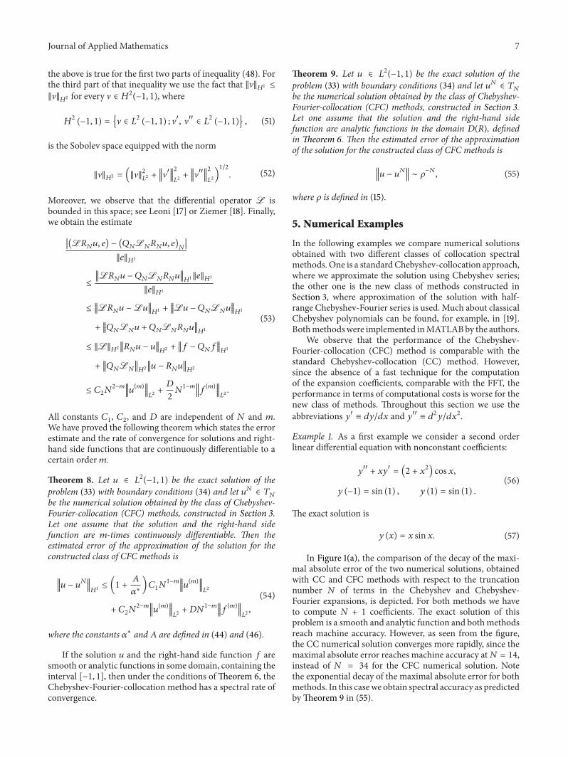