research article …chromy/sps2/referaty/80 - average bandwidth... · research article ......

Hindawi Publishing CorporationModelling and Simulation in EngineeringVolume 2012, Article ID 301012, 7 pagesdoi:10.1155/2012/301012

Research Article

Average Bandwidth Allocation Model of WFQ

Tomas Balogh and Martin Medvecky

Institute of Telecommunications, Faculty of Electrical Engineering and Information Technology, Slovak University of Technology,Ilkovicova 3, 812 19 Bratislava, Slovakia

Correspondence should be addressed to Tomas Balogh, [email protected]

Received 12 April 2012; Revised 21 October 2012; Accepted 5 November 2012

Academic Editor: Agostino Bruzzone

Copyright © 2012 T. Balogh and M. Medvecky. This is an open access article distributed under the Creative Commons AttributionLicense, which permits unrestricted use, distribution, and reproduction in any medium, provided the original work is properlycited.

We present a new iterative method for the calculation of average bandwidth assignment to traffic flows using a WFQ schedulerin IP based NGN networks. The bandwidth assignment calculation is based on the link speed, assigned weights, arrival rate, andaverage packet length or input rate of the traffic flows. We prove the model outcome with examples and simulation results usingNS2 simulator.

1. Introduction

The current trends in telecommunication infrastructurewith packet oriented networks bring up the question ofsupporting Quality of Service (QoS). Methods, that are ableto assign priorities to flows or packets and then servicethem differently according to their needs in network nodes,were proposed for the demands of QoS support. QueueScheduling Discipline (QSD) algorithms are responsible forchoosing packets to output from queues. They are designedto divide the output capacity fairly and optimally. Algorithmsthat are able to make this decision according to priorities arethe basic component of modern QoS supporting networks[1].

For an optimal configuration of these algorithms we needto calculate or simulate the result of our setting to expect theimpact on QoS. The network nodes can be modeled usingMarkovian models [2].

Most of the existing WFQ bandwidth allocation modelsdo not consider variable utilization of queues or bandwidthredistribution of unassigned link capacity. For this reason weproposed our iterative mathematical model for bandwidthallocation of WFQ. The model can be used for the analysisof the impact of weight settings, analyzing the stability ofthe system and modeling of delay and queue length of trafficclasses.

The next sections of the paper are structured as follows.At first the WFQ algorithm is presented followed by a short

presentation of common used bandwidth constraint models.The third section of the paper describes the proposedmodel for average bandwidth allocation of WFQ followedby examples of WFQ bandwidth allocation and simulationresults proving the proposed model.

2. Bandwidth Allocation

There are many scheduling algorithms and several band-width allocation models proposed for bandwidth allocationestimation. We focused on WFQ and bandwidth allocationmodels proposed for MPLS traffic engineering.

2.1. Weighted Fair Queuing. WFQ was introduced in 1989by Demers et al. and Zhang [3, 4]. The algorithm providesfair output bandwidth sharing according to assigned weights.The decision which packet should be read from the packetqueue and sent next is done by calculating a virtual finish-time. The scheduler assigns the finish time to each packetas it arrives in the queue. The time corresponds with thetime, in which the packet would be completely sent bit bybit from each queue as in the Generalized Processor Sharing(GPS) algorithm. The number of bits calculated in one turncorresponds with the assigned weights. The packet with thesmallest finish time is chosen for output. WFQ guaranteesthat each traffic class gets a portion of the output bandwidthand shares it proportional to the assigned weights.

2 Modelling and Simulation in Engineering

2.2. Bandwidth Constraint Models. One of the goals of Diff-Serv or MPLS traffic engineering is to guarantee bandwidthreservations for different service classes. For these goals twofunctions are defined [5]:

(i) class-type (CT) is a group of traffic flows, based onQoS settings, sharing the same bandwidth reserva-tion;

(ii) bandwidth constraint (BC) is a part of the outputbandwidth that a CT can use.

For the mapping between BCs and CTs the maximumallocation model (MAM), max allocation with reservation(MAR), and Russian dolls model (RDM) are defined.

Maximum Allocation Model. The MAM model [6] maps oneBC to one CT. The whole bandwidth is strictly divided andno sharing between CTs is allowed.

Max Allocation with Reservation. MAR [7] is similar toMAM in that a maximum bandwidth is allocated to eachCT. However, through the use of bandwidth reservationand protection mechanisms, CTs are allowed to exceed theirbandwidth allocations under conditions of no congestionbut revert to their allocated bandwidths when overload andcongestion occurs [6].

Russian Dolls Model. The RDM model is more effective inbandwidth sharing. It assigns BCs to groups of CTs. Forexample CT7 with the highest QoS requirements gets its ownBC7. The CT6 with lower QoS requirements shares its BC6with CT7, and so forth. In extreme cases the lower prioritiesget less bandwidth as they need or even starve [8].

3. WFQ Bandwidth Allocation Model

In general, WFQ and some other scheduling algorithms likeWRR, WF2Q+, and so forth allocate bandwidth differently asthe models described in Section 2.2. The available bandwidthis divided between service classes or waiting queues accord-ing to assigned weights. The sharing of unused bandwidthis allowed and is divided between the other queues againaccording to assigned weights.

The proposed model is a part of the research of modellingof traffic parameters of NGN networks, is a modificationa presented model for bandwidth allocation of the WRRalgorithm, and will be further used for delay and queuelength modeling of these algorithms.

3.1. Definitions and Notations. We assume a network nodewith P priority classes or waiting queues. Each queue i has aweight wi assigned. Packets enter the queue with an arrivalrate λi and mean packet size Li. The product of these twovariables represents the input bandwidth of the priority:

Ii = λiLi. (1)

The total available output bandwidth T will be dividedbetween the priority classes and each of them will get Bi.

For the bandwidth calculation an iterative method will beused. The kth iteration of Bi will be noted as Bi,k.

3.2. Model Proposal. To describe the bandwidth allocationof WFQ, we have to analyze all possible situations that canoccur. We will use an iterative method for the analysis.

Let us take a look at the possible situations that canappear in the first step of bandwidth allocation. The WFQalgorithm works at the principle that a number of bitsrepresented by the weight value are sent at once to a virtualoutput. The bits are then reorganized to the original packetsand the packet which is completely transmitted in this wayis dequeued as the first. This assures an exact bandwidthallocation between queues according to assigned weights.The distribution of the available bandwidth can be writtenas follows:

Twi

∑Pj=1 wj

. (2)

After the bandwidth is divided between the queuesaccording to (2), there are 3 possible situations.

(i) The first possibility is that each queue gets anduses the bandwidth calculated in (2). No additionalsharing of unused bandwidth will happen. This willhappen if

Twi

∑Pj=1 wj

≤ λiLi = Ii, i = 1, 2, . . . ,P. (3)

(ii) The second option is that each queue is satisfied withthe assigned bandwidth. In this case:

Twi

∑Pj=1 wj

≥ λiLi = Ii, i = 1, 2, . . . ,P. (4)

In these two cases, the bandwidth assignment is finishedin the first iteration step. No unused bandwidth needs to bedivided between other queues. A queue gets the bandwidthwhich it needs (1) or the proportion of bandwidth based onthe WFQ rules (2):

Bi,1 = min

⎛

⎝Ii,Twi

∑Pj=1 wj

⎞

⎠. (5)

This (5) represents also our first iteration step.If the conditions (3) or (4) are not met, we have to

calculate the bandwidth assignment in the next iterationsteps. This means some queues need more bandwidth thanhas been assigned using (2), some others use only thebandwidth calculated in (1), and the rest of the bandwidthis unused and can be shared. We will reassign the unusedbandwidth only between the queues whose requirements arenot satisfied. The queues that do not need more bandwidthcan be identified as follows:

Ii − Bi,k−1 = 0. (6)

If the queues bandwidth requirements are met, the resultof (6) will be zero. On the other hand a positive number

Modelling and Simulation in Engineering 3

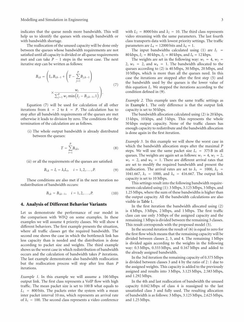
indicates that the queue needs more bandwidth. This willhelp us to identify the queues with enough bandwidth orwith bandwidth shortage.

The reallocation of the unused capacity will be done onlybetween the queues whose bandwidth requirements are notsatisfied until all capacity is divided or all queue requirementsmet and can take P − 1 steps in the worst case. The nextiterative step can be written as follows:

Bi,k =⎛

⎝Ii,Bi,k−1 +

⎛

⎝T −P∑

j=1

Bj,k−1

⎞

⎠

× wi∑P

j=1 wj min(I j − Bj,k−1, 1

)

⎞

⎠.

(7)

Equation (7) will be used for calculation of all otheriterations from k = 2 to k = P. The calculation has tostop after all bandwidth requirements of the queues are metotherwise it leads to division by zero. The conditions for thetermination of the calculation are as follows.

(i) The whole output bandwidth is already distributedbetween the queues:

T =P∑

i=1

Bi,k, (8)

(ii) or all the requirements of the queues are satisfied:

Bi,k = Ii = λiLi, i = 1, 2, . . . ,P. (9)

These conditions are also met if in the next iteration noredistribution of bandwidth occurs:

Bi,k = Bi,k−1, i = 1, 2, . . . ,P. (10)

4. Analysis of Different Behavior Variants

Let us demonstrate the performance of our model inthe comparison with WFQ on some examples. In theseexamples we will assume 4 priority classes. We will show 4different behaviors. The first example presents the situation,where all traffic classes get the required bandwidth. Thesecond one shows the case in which the bottleneck link hasless capacity than is needed and the distribution is doneaccording to packet size and weights. The third exampleshows us the worst case in which redistribution of bandwidthoccurs and the calculation of bandwidth takes P iterations.The last example demonstrates also bandwidth reallocationbut the reallocation process will stop after less than Piterations.

Example 1. In this example we will assume a 100 Mbpsoutput link. The first class represents a VoIP flow with hightraffic. The mean packet size is set to 100 B what equals toL1 = 800 bits. The packets enter the system with a meaninter packet interval 10 ms, which represents an arrival rateof λ1 = 100. The second class represents a video conference

with L2 = 8000 bits and λ2 = 10. The third class representsvideo streaming with the same parameters. The last fourthclass transports data with lowest priority settings. The trafficparameters are L4 = 12000 bits and λ4 = 1.

The input bandwidths calculated using (1) are I1 =80 kbps, I2 = 80 kbps, I3 = 80 kbps, and I4 = 12 kbps.

The weights are set in the following way: w1 = 4, w2 =2, w3 = 2, and w4 = 1. The bandwidth allocated to thequeues according to (2) is 40 Mbps, 30 Mbps, 20 Mbps, and10 Mbps, which is more than all the queues need. In thiscase the iterations are stopped after the first step (5) andthe bandwidth used by the queues is the lower value ofthis equation Ii. We stopped the iterations according to thecondition defined in (9).

Example 2. This example uses the same traffic settings asin Example 1. The only difference is that the output linkcapacity is set to 50 kbps.

The bandwidth allocation calculated using (2) is 20 kbps,15 kbps, 10 kbps, and 5 kbps. This represents the whole50 kbps output capacity. None of the traffic classes hasenough capacity to redistribute and the bandwidth allocationis done again in the first iteration.

Example 3. In this example we will show the worst case inwhich the bandwidth allocation stops after the maximal Psteps. We will use the same packet size Li = 375 B in allqueues. The weights are again set as follows: w1 = 4, w2 = 2,w3 = 2, and w4 = 1. There are different arrival rates thatare set to modify the required bandwidth and present thereallocation. The arrival rates are set to λ1 = 1000, λ2 =1041.667, λ3 = 1000, and λ4 = 416.667. The output linkcapacity is set to 10 Mbps.

This settings result into the following bandwidth require-ments calculated using (1): 3 Mbps, 3.125 Mbps, 3 Mbps, and1.25 Mbps, where the sum of these bandwidths is higher thanthe output capacity. All the bandwidth calculations are alsovisible in Table 1.

In the first iteration the bandwidth allocated using (2)is 4 Mbps, 3 Mbps, 2 Mbps, and 1 Mbps. The first trafficclass can use only 3 Mbps of the assigned capacity and theremaining 1 Mbps is divided between the remaining 3 classes.This result corresponds with the proposed model (5).

In the second iteration the result of (6) is equal to zero forthe first flow which means that the remaining capacity will bedivided between classes 2, 3, and 4. The remaining 1 Mbpsis divided again according to the weights in the followingway: 0.5 Mbps, 0.333 Mbps, and 0.167 Mbps and added tothe already assigned bandwidth.

In the 3rd iteration the remaining capacity of 0.375 Mbpsis divided between classes 3 and 4 by the ratio of 2 : 1 due tothe assigned weights. This capacity is added to the previouslyassigned and results into 3 Mbps, 3.125 Mbps, 2.583 Mbps,and 1.292 Mbps.

In the 4th and last reallocation of bandwidth the unusedcapacity 0.042 Mbps of class 4 is reassigned to the lastunsatisfied class 3 and fully used. The resulting allocationof bandwidth is as follows: 3 Mbps, 3.125 Mbps, 2.625 Mbps,and 1.25 Mbps.


Table 1: Allocation of bandwidth in Example 3.

Traffic class

Bandwidth

Required (Mpbs)1st iteration 2nd iteration 3rd iteration 4th iteration

Allocated(Mpbs)

Unallocated(Mpbs)

Allocated(Mpbs)

Unallocated(Mpbs)

Allocated(Mpbs)

Unallocated(Mpbs)

Allocated(Mpbs)

Traffic class 1 3 4 1 3 3 3

Traffic class 2 3.125 3 3.5 0.375 3.125 3.125

Traffic class 3 3 2 2.333 2.583 2.625

Traffic class 4 1.25 1 1.167 1.292 0.045 1.25

All these results correspond with the proposed models(5) and (7).

Example 4. This example describes the bandwidth alloca-tion, where the calculation has to be stopped after theconditions in (8) or (9) are met.

The weight and packet size settings are the same as inthe previous Example 3. The output bandwidth is set againto 10 Mbps. The arrival rates are set to 1000, 1000, 750,and 500 pps (packets per second). These settings lead tobandwidth requirements of 3, 3, 2.25, and 1.5 Mbps as aresult of (1).

In the first iteration using (2) we allocate 4, 3, 2, and1 Mbps to the queues. In this case the first queue has 1 Mbpsremaining for reallocation and the second queue is alreadysatisfied with the allocated bandwidth.

The second iteration reassigns the 1 Mbps divided usingthe ratio 2 : 1 to queues 3 and 4. The bandwidth assignedto them is 2.667 Mbps and 1.333 Mbps, but queue 3 needsonly 2.25 Mbps output capacity and the remaining part ofthe capacity can be reassigned to the last unsatisfied queue 4.

In the third iteration we assign 3 Mbps to the first queue,2 Mbps to the second queue, 2.25 Mbps to the third queue,and 1.75 Mbps to the last queue. The fourth queue needs only1.5 Mbps and this means that bandwidth requirements of allqueues are met. The iterations have to stop at this momentaccording to (9) otherwise the model would lead to dividingby zero.

We can change the arrival rate of the fourth queue to750 pps and raise the bandwidth requirements 2.25 Mbps.In this case in the 3rd iteration the bandwidth allocationsare 3, 3, 2.25, and 1.75 Mbps. This means that the wholeoutput capacity is divided to the queues (8) and we can stopthe iteration. Otherwise each next step would lead to sameresults.

5. Simulations

To proove the results of our mathematical model we usedsimulations in the NS2 simulation software [9] (version 2.29)with DiffServ4NS patch [10].

For the simulations a simple network model with 4transmitting nodes (1–4) and four receiving nodes (6–9) was used. The transmitting and receiving nodes areinterconnected with one link between nodes 0 and 5. Thenode 0 uses WFQ to schedule packets on this bottleneck link

0

1

2

3

4

5

6

7

8

9

Bottleneck

100 Mbps

100 Mbps

100 Mbps100 Mbps

100 Mbps

100 Mbps

100 Mbps

100 Mbps

Figure 1: Simulation model.

where the mentioned bandwidths are set. All other links havea capacity of 100 Mbps. The model is shown in Figure 1. Thequeues at node 0 have enough capacity so no packet loss willoccur.

We used two types of traffic sources. The first onegenerates packets only with one packet size and constantpacket interval. These settings are easier to simulate andrepresent a D/D/1/∞Markovian model.

The second traffic source type represents an M/M/1/∞model. There is a lack of possibility to generate trafficswith different packet sizes in NS2 simulator. For this reasonthe M/M/1 source is modeled using an ON/OFF sourcewhere each node generates one packet with a random size(exponential distribution) and the interval for the nextpacket transmission is a random time (again a randomnumber with exponential distribution).

An example of input data generated at one node with themean packet size 375 B and arrival rate 1000 pps is shown inFigures 2 and 3. The red line represents the number of pack-ets generated corresponding with the exponential probabilitycalculated for these settings and the blue bars represent thehistogram of packets generated in the simulation that lasted100 s.

We made many simulations under different parametersettings. The presented results correspond with describedexamples or present different extreme settings. The results ofsimulations of M/M/1 and D/D/1 models and the results ofour proposed model are shown in Table 2.

We measured the bandwidth after achieving “steadystate.” The measurement started after 20 s of simulation whenthe bandwidth was stable and queues filled up with waitingpackets [11].


Ta

ble

2:Si

mu

lati

onre

sult

sco

mpa

red

wit

hm

ath

emat

ical

mod

elre

sult

s.

Sim

ula

tion

vari

ant

(#)

(1)

(2)

(3)

(4)

(5)

(6)

(7)

(8)

(9)

Mea

npa

cket

size

(B)

100,

1000

,10

00,1

500

100,

1000

,100

0,15

0037

5,37

5,37

5,37

537

5,37

5,37

5,37

537

5,37

5,37

5,37

510

00,1

00,1

0,1

1000

,100

0,10

00,1

000

1000

,100

,100

0,10

010

00,1

000,

1000

,100

0M

ean

arri

val

rate

(pps

)10

0,10

,10,

110

0,10

,10,

110

00,1

041.

67,

1000

,416

.67

1000

,100

0,75

0,50

010

00,1

000,

750,

750

100,

100,

100,

100

1,10

,10

0,10

0010

00,1

00,1

000,

100

100,

100,

100,

100

Inpu

tba

ndw

idth

(Mbp

s)

0.08

,0.0

8,0.

08,

0.01

20.

08,0

.08,

0.08

,0.

012

3,3.

125,

3,1.

253,

3,2.

25,1

.53,

3,2.

25,2

.25

0.8,

0.08

,0.0

08,

0.00

080.

008,

0.08

,0.8

,8

8,0.

08,

8,0.

080.

8,0.

8,0.

8,0.

8

Wei

ght

sett

ings

4,3,

2,1

4,3,

2,1

4,3,

2,1

4,3,

2,1

4,3,

2,1

1,1,

1,1

4,3,

2,1

4,3,

2,1

40,3

,2,1

Lin

kca

paci

ty(M

bps)

100

0.05

1010

100.

54

81.

6

D/D

/1si

mu

lati

onre

sult

s(M

bps)

0.07

9,0.

079,

0.07

9,0.

012

0.01

9,0.

015,

0.01

,0.0

053.

00,3

.15,

2.59

,1.

248

2.99

,2.9

9,2.

249,

1.50

2.99

,3.0

0,2.

25,

1.74

90.

41,0

.08,

0.00

79,0

.000

80.

0078

,0.0

8,0.

8,3.

111

5.22

6,0.

079,

2.61

33,0

.079

0.79

,0.4

,0.2

67,

0.13

3

M/M

/1si

mu

lati

onre

sult

s(M

bps)

0.08

04±

0.47

%0.

0200±

0.06

%3.

0041±

0.13

%3.

0061±

0.43

%3.

0054±

0.34

%0.

4095±

0.21

%0.

0080±

2.73

%5.

2261±

0.01

%0.

8015±

0.56

%0.

0801±

1.34

%0.

0150±

0.10

%3.

1296±

0.14

%3.

0022±

0.23

%3.

0030±

0.13

%0.

0808±

1.07

%0.

0799±

0.97

%0.

0804±

0.42

%0.

3993±

0.57

%0.

0802±

1.26

%0.

010±

0.12

%2.

6134±

0.30

%2.

2501±

0.32

%2.

2564±

0.21

%0.

0085±

1.01

%0.

7991±

0.67

%2.

6131±

0.07

%0.

2662±

0.57

%0.

0122±

1.69

%0.

0050±

0.36

%1.

2529±

0.27

%1.

5007±

0.33

%1.

7352±

0.66

%0.

0013±

0.77

%3.

1129±

0.17

%0.

0805±

0.57

%0.

1331±

0.56

%M

odel

resu

lts

(Mbp

s)0.

08,0

.08,

0.08

,0.

012

0.02

,0.0

15,

0.01

,0.0

053,

3.12

5,2.

625,

1.25

3,3,

2.25

,1.5

3,3,

2.25

,1.7

50.

411,

0.08

,0.

008,

0.00

080.

008,

0.08

,0.8

,3.

112

5.22

66,0

.08,

2.61

33,0

.08

0.8,

0.4,

0.26

6,0.

133


0 0.5 1 1.5 2 2.5 3 3.5 4 4.5 50

1000

2000

3000

4000

5000

6000

7000

8000

9000

10000

Packet interval (s)

Nu

mbe

r of

gen

erat

ed p

acke

ts

×10−3

Figure 2: Exponential probability distribution of arrival rate withmean value 1000 pps.

0 200 400 600 800 1000 1200 1400 1600 1800 20000

1000

2000

3000

4000

5000

6000

Packet size (B)

Nu

mbe

r of

gen

erat

ed p

acke

ts

Figure 3: Exponential probability distribution of packet sizes withmean value 375 B.

The results of the mathematical model mostly corre-spond with the simulation results. The results of the D/D/1simulation model are more exact due to the exact settingof packet size. The small inaccuracy can be caused bymeasurement errors, where the bandwidth calculation isstopped closely to an arrival of a packet when small arrivalrates are set. Due to the deterministic parameter settingsthere is no difference between more runs of simulations andno result variance occurs.

The presented results for the M/M/1 simulations arean average value calculated from 10 simulation runs andthe standard deviation of the runs is also provided. Thesimulation runs for most parameter settings lasted 200 s.In cases an extreme low arrival rate was set we extendedthe simulation duration up to 1000 s. We provided alsosimulations with WF2Q+ [12] scheduler instead of WFQ.The simulation results correspondent with the presentedresults and proved that this model is applicable also for otherWFQ based schedulers that use packet size for the dequeueorder decision.

6. Conclusion

We presented a new iterative bandwidth allocation modelfor WFQ in IP based NGN networks. The proposed modeluses the weight settings of the WFQ scheduler and averageinput bandwidth of different flows for the bandwidthcalculation. The variable utilization of different queues andpacket redistribution is considered in the calculations. Theproposed model allows to easily predict the impacts of thescheduler, traffic shapers, and input traffics on QoS of thetransported data.

The functionality of the model was presented on fivedifferent examples and confirmed by simulations in the NS2simulator for both D/D/1 and M/M/1 input traffics.

The proposed iterative bandwidth allocation model wastested with WF2Q+ scheduler with the same simulationresults. Therefore we can say that proposed model is alsoapplicable on other WFQ based schedulers.

The results of this bandwidth allocation model will beused in further research of delay and packet loss modelingusing Markovian queue models.

Acknowledgments

This work is a part of research activities conducted atSlovak University of Technology Bratislava, Faculty of Elec-trical Engineering and Information Technology, Instituteof Telecommunications, within the scope of the project“Support of Center of Excellence for SMART Technologies,Systems and Services II., ITMS 26240120029, cofunded bythe ERDF.”

References

[1] T. Misuth and I. Barona, “On queueing systems application inIP networks,” in EE CAsopis Pre Elektrotechniku A Energetiku,vol. 16, pp. 91–94, 2010.

[2] T. Misuth, E. Chromy, and M. Kavacky, “Prediction of trafficin the contact centers,” in Proceedings of the 6th Interna-tional Conference on Electrical and Electronics Engineering(ELECO’09), pp. 111–114, Bursa, Turkey, November 2009.

[3] A. Demers, S. Keshav, and S. Shenker, “Analysis and simulationof a fair queuing algorithm,” in Proceedings of the ACMComputer Communication Review (SIGCOMM ’89), pp. 3–12,1989.

[4] L. Zhang, “Virtual clock: a new traffic control algorithmfor packet switching networks,” in Proceedings of the ACMTransactions on Computer Systems, vol. 9, no. 2, pp. 101–124,1990.

[5] K. Molnar and M. Vlcek, “Evaluation of bandwidth constraintmodels for MPLS networks,” Electronics, vol. 1, pp. 172–175,2009.

[6] RFC, 4125, Maximum Allocation Bandwidth Constraints Modelfor DiffServ-Aware MPLS Traffic Engeneering, The InternetSociety, 2005.

[7] RFC, 4126, Max Allocation with Reservation Bandwidth Con-straints Model for Diffserv-Aware MPLS Traffic Engineering &Performance Comparisons, The Internet Society, 2005.

[8] RFC, 4127, Russian Dolls Bandwidth Constraints Model forDiffServ-Aware MPLS Traffic Engeneering, The Internet Soci-ety, 2005.


[9] The Network Simulator-ns-2, http://www.isi.edu/nsnam/ns/.[10] Andreozzi, “Sergio. DiffServ4NS,” http://sergioandreozzi

.com/research/network/diffserv4ns/.[11] K. Pawlikowski, H. D. J. Jeong, and J.S. R. Lee, “On credibility

of simulation studies of telecommunication networks,” IEEECommunications Magazine, vol. 40, no. 1, pp. 132–139, 2002.

[12] J. C. R. Bennet and H. Zhang, “Hierarchical packet fair queu-ing algorithms,” in Proceedings of the IEEE/ACM Transactionson Networking, pp. 675–689, 1997.

Submit your manuscripts athttp://www.hindawi.com

VLSI Design

Hindawi Publishing Corporationhttp://www.hindawi.com Volume 2014

International Journal of

RotatingMachinery


Hindawi Publishing Corporation http://www.hindawi.com

Journal ofEngineeringVolume 2014


Shock and Vibration


Mechanical Engineering

Advances in


Civil EngineeringAdvances in

Acoustics and VibrationAdvances in



Electrical and Computer Engineering

Journal of


Distributed Sensor Networks


The Scientific World JournalHindawi Publishing Corporation http://www.hindawi.com Volume 2014

SensorsJournal of


Modelling & Simulation in EngineeringHindawi Publishing Corporation http://www.hindawi.com Volume 2014


Active and Passive Electronic Components


Chemical EngineeringInternational Journal of

Control Scienceand Engineering

Journal of


Antennas andPropagation




Navigation and Observation


Advances inOptoElectronics

Hindawi Publishing Corporation http://www.hindawi.com

Volume 2014

RoboticsJournal of


research article …chromy/sps2/referaty/80 - average bandwidth... · research article ......

Documents