research article condition assessment of pc...

Research ArticleCondition Assessment of PC Tendon Duct Filling byElastic Wave Velocity Mapping

Kit Fook Liu,1 Hwa Kian Chai,1 Nima Mehrabi,1

Kobayashi Yoshikazu,2 and Tomoki Shiotani3

1 Department of Civil Engineering, University of Malaya, Kuala Lumpur, Malaysia2 Department of Civil Engineering, Nihon University, Tokyo, Japan3 Graduate School of Engineering, Kyoto University, Kyoto, Japan

Correspondence should be addressed to Hwa Kian Chai; [email protected]

Received 12 November 2013; Accepted 16 December 2013; Published 6 March 2014

Academic Editors: A. Esmaeily, B. Kumar, and A. Rodrıguez-Castellanos

Copyright © 2014 Kit Fook Liu et al. This is an open access article distributed under the Creative Commons Attribution License,which permits unrestricted use, distribution, and reproduction in any medium, provided the original work is properly cited.

Imaging techniques are high in demand for modern nondestructive evaluation of large-scale concrete structures. The travel-timetomography (TTT) technique, which is based on the principle of mapping the change of propagation velocity of transient elasticwaves in a measured object, has found increasing application for assessing in situ concrete structures. The primary aim of thistechnique is to detect defects that exist in a structure. The TTT technique can offer an effective means for assessing tendon ductfilling of prestressed concrete (PC) elements. This study is aimed at clarifying some of the issues pertaining to the reliability of thetechnique for this purpose, such as sensor arrangement, model, meshing, type of tendon sheath, thickness of sheath, and materialtype as well as the scale of inhomogeneity. The work involved 2D simulations of wave motions, signal processing to extract traveltime of waves, and tomography reconstruction computation for velocity mapping of defect in tendon duct.

1. Introduction

Prestressed concrete (PC) is recognized as a vital technologyto overcome concrete’s natural weakness in tension especiallyfor bridge structure. However, improper grouting of tendonduct can lead to deterioration inside the bridge structurewhich includes cracking and corrosion of tendons. Thecorrosion in tendon duct leads to lack of cross-sectionalarea and increases stress to the other tendons, finally resultsin bridge collapse [1]. To avoid collapse of a deterioratedstructure or other disaster, proper preventive maintenancehas to be carried out. Nondestructive testing has to be carriedout to detect which part of bridge structure is defected so thatrepair work can be carried out rapidly and cost efficiently.Besides, it is encouraged to conduct inspection on a regularbasis so that necessary considerations and effective repairaction can be implemented.There are various nondestructivetechniques (NDT) that have been practiced by engineers in

detecting defects and evaluating the integrity of structuresdepending on the physical conditions of concrete structures.NDT is a group of techniques that evaluate the propertiesof material, component, or system without impairing itsfuture usefulness. The unique advantages of employing NDTinclude time and cost saving, flexibility in operation, andsimple implementation. The results are useful in providingwarning or indication towards imminent failure.

NDT is a very demanding profession for assessmentof concrete structures because destructive methods such ascoring and drilling will leave permanent damage and arecostly. Also, defects that are left by destructive methodspotentially become focal points for deterioration. SeveralNDT methods have been used so far for assessment of PC,which include impact-echo, radar technique, radioactive, andimpulse thermography. The impact-echo method employselastic wave to propagate in concrete structure and elasticwave will reflect on concrete surface when it meets with

Hindawi Publishing Corporatione Scientific World JournalVolume 2014, Article ID 194295, 14 pageshttp://dx.doi.org/10.1155/2014/194295

2 The Scientific World Journal

internal defects. This method is applied to pre- and postten-sioned concrete structure to determine the location of thedefect. For impact-echo method, it is essential to ensure thatimpact frequency is sufficiently high to identify the defect.However this technique is not always accurate because manypeak frequencies are observed in the frequency spectra dueto reflection, diffraction, and so forth. To circumvent this,a new procedure was developed by applying an imagingprocedure to the impact-echo data, as stack imaging ofspectral amplitudes based on impact-echo (SIBIE) [2, 3].Alver and Ohtsu had conducted lab tests regarding SIBIEprocedure which is found to be efficient to identify specimenscontaining grouted and ungrouted ducts [4].The state-of-theart ultrasonic tomography (MIRA) is a device manufacturedby Acoustic Control Systems, which contains four rows ofsensors in which each row contains ten transducers. Theimpact-echo needs one receiver sensor for one measure-ment, while the MIRA used the same concept as impact-echo. MIRA is an ultrasonic tomography device that wasdeveloped to determine the depth of concrete pavementand reinforcement location as well as detection of flaws inconcrete pavement or PC. However, it is suggested to use theMIRAwith combination of other NDT techniques because ofthe inability of the device to determine the exact location offlaws at big areas by short time [5]. On the other hand, radartechnique such as the electromagnetic (EM) wave methodcan be rapid to locate and image defects inside of concretestructures effectively. However, radar techniques are foundto have imaging limitations such as diffraction which mightaffect the visualization, lack of exact inversion algorithms,loss of polarization information due to scalar inversion, andhigh attenuation of EM waves in moisture [6]. There areexperiments which were conducted by Langenberg et al. toassess the condition of PC tendon duct by using EM wave;generally the EM waves face the problem of being shieldedby the steel grid and the tendon duct itself [7]. Radioactivemethods such as X-ray can provide high resolution result oftendon duct images as X-ray is nondiffracting and possesseshigh penetration capability. But there are limitations for X-ray methods such as high operating costs and safety issuesdue to risk of radiation. Impulse thermography can beapplied to detect subsurface defects of tendon duct, eitherby heat hydration of the grout, infrared array, or electricresistance. Defects can be identified when there are areas ofdifferent temperatures as a result of transient heat transfer.This method is effective for penetration up to 10 cm, andidentification is good only at an early stage of concretehardening [8]. But, Clark et al. found that weather and surfaceconditions can affect the accuracy of imaging by impulsethermography [9].

In this study, the NDT method in focus is the travel-time tomography (TTT) reconstruction technique, whichprovides assessment through variation of travel time ofelastic waves from a source to multiple receivers locatedat different locations of the target structure. The traveltime, or inversely the velocity of elastic wave, depends onthe medium of propagation. The governing properties thatinfluence the behaviour of propagation include density andacoustic impedance, as well as homogeneity of the material

[10–14]. According to Vergara et al. [15], wave propagation isalso affected by inhomogeneity in the forms of porosity andaggregates in concrete. For assessment purposes, there areestablished empirical correlations between wave velocity andconcrete quality [16, 17]. Commonly, velocities higher than3500ms−1 indicate sound concrete, while those lower than3500ms−1 are common in normal concrete with questionableintegrity [18]. The delay or low velocity of observed data canalways be associated with the presence of an anomaly ordefect, in the form of cracking or voiding.

A significant merit for TTT method in civil structuresmaintenance industry is that the tomography results can bekept as an appraisal record for new construction and as asource of reference to evaluate the status of deteriorationor damage during the service period [18]. In order toincrease the reliability of TTT assessment and to confirmproper instrumentation andmeasurement configuration, it isoften necessary to conduct wave motion simulation becausethe size, material characteristics, and geometry of concretestructures are varied from one to another. Simulation workis necessary to obtain important information such as opti-mum conditions for sensor arrangement and frequency ofthe wave. Likewise, through simulation, decisions can bemade in terms of the required number of sensors, requiredassessment sides of the structure, and the size of meshingfor satisfactory visualization to ensure cost-effectiveness ofmeasurement. Beside velocity variation, attenuation of elasticwaves is considered to be a more sensitive variation againsthomogeneity. Nevertheless, due to significant attenuation ofelastic waves through cementitious medium especially withdefects, the velocity and attenuation tomography might notbe suitable for utilizing on large scale structure becauseof the loss of signal amplitude even in concrete free ofdefect. Attenuation is also considered very dependent onthe coupling and surface conditions, while velocity is not asmuch [19].

1.1. Tomography by Travel Time of Elastic Waves. The TTT isa type of transmission tomography technique that employselastic waves to propagate on the target structure mediumfrom one source tomultiple receivers as shown in Figure 1(a).The inversion of travel-time data enables for tomographicimaging of the velocity distribution within the sampledstructure. It is known that elastic waves propagate at varyingvelocities in different materials and are highly dependableupon the physical properties of the medium, such as elasticmodulus and acoustic impedance of laying materials. Thisis because when there is heterogeneity in a medium orexistence of voids, the elastic waveswill experience scattering,reflection, and diffraction; in such a loss of energy theproperties of waves such as frequencies and amplitude maychange [20]. This method allows better identification ofanomalous regions by performing an inversion of boundarymeasurements to determine the physical properties withinthe body of a structure. The visualization of tomogramshould be highly presentable and easy to be understoodnot only by NDT engineers but also by people without therelevant technical background, such as owners of structures.

The Scientific World Journal 3

Anomaly

Source

Source

Receivers

Receivers

(a)

A

B

(b)

Figure 1: (a) Schematic illustration of anomaly projections with ray trace from source nodal to multiple receivers [1]; (b) an example ofone-ray traces from point 𝐴 to point 𝐵 based on illustration (a).

The following section describes inversion of travel-time datawhich has been practiced by this experiment.

Based on the ray theory, the travel time 𝑡, for the wave totravel from source 𝐴 to receiver 𝐵 (as in Figure 1) is given bythe path integral [18]:

Travel time, 𝑡 = ∫

𝐵

𝐴

1

V𝑑𝑙 = ∫

𝐵

𝐴

𝑠 𝑑𝑙, (1)

where the integral follows the ray path from point 𝐴 to point𝐵 with V as velocity, 𝑠 is the wave slowness (also known asreciprocal of velocity), and 𝑑𝑙 is the element length. Basedon the series expansion technique, 𝑠(𝑥, 𝑧) as a set of discreteelements or pixels, each with a uniform slowness, 𝑠

𝑗

(𝑗 =

1,𝑀, where 𝑀 is the number of pixels). Then the integralcorresponding to travel time, 𝑡

𝑖

(𝑖 = 1,𝑁, where 𝑁 is thenumber of observations) becomes a summation:

𝑡𝑖

=

𝑀

∑

𝑗=1

𝑝𝑗

𝑑𝑖𝑗

(𝑖 = 1, . . . , 𝑁) , (2)

where 𝑑𝑖𝑗

is the distance travelled by ray 𝑖 in pixel 𝑗. Forthe whole set of rays, the travel time equation above can berepresented in matrix form as

𝑇 = 𝐷𝑃, (3)

where 𝑇 and 𝑃 are column vectors of length 𝑁 and 𝑀,respectively, and 𝐷 is an 𝑁 by 𝑀 rectangular matrix. Meshvelocity of tomogram are results from solving the slownessvector, 𝑃 from observation travel time matrix, 𝑇 and path

length, 𝐷. To solve the slowness vector 𝑃, it is required tomeasure travel time, 𝑇, and transpose matrix𝐷

∗:

𝑃 = 𝐷∗𝑇

𝑇, (4)

where the matrix 𝐷∗ is obtained by dividing each row of 𝐷,

corresponding to a particular ray path, by the square of thepath length. Thus,

𝑃𝑗

=

𝑁

∑

𝑖=1

𝐷𝑖𝑗

𝑇𝑖

𝐷2

𝑖

(𝑗 = 1, . . . ,𝑀) . (5)

The Equation (5) can be expressed as matrix form inEquation (6) and it can be solved until it satisfies theinconsistent data as closely as possible.

𝑃 = (𝐷𝑇

𝐷)−1

𝐷𝑇

𝑇. (6)

Since this group of matrix involves a high amount oforder and value, the simultaneous iterative reconstructiontechniques (SIRT) program is developed to reconstruct thevelocity distribution across the structure.

In this research, wave motion simulation was used togenerate data for the TTT method in assessing the fillingof the PC tendon duct. The objective of this study is toinvestigate the effect of sensors arrangement, mesh size andnumber of elements, material of tendon sheath, and thicknessof tendon sheath on the reliability of TTT measurement.Discussion is also extended to analyse the TTT results forquantitative evaluation of filling.


2. Methodology

2.1. Numerical Simulations. The analytical work was car-ried out by two-dimensional (2D) numerical simulations ofwave motions. The numerical simulations were conductedwith commercially available software named Wave2000 Plusdeveloped by CyberLogic, Inc., in order to produce theraw data (travel time). The simulation results were furtherprocessed and the data were used as the input data fortomography reconstruction computation to generate tomo-grams that indicate the velocity distribution of the interiorof the measured target. The fundamental equation of two-dimensional propagation of stress waves in a perfectly elasticmedium, by ignoring viscous losses, is as follows:

𝑝𝜕2

𝑢

𝜕𝑡2= 𝜇∇2

𝑢 + (𝜆 + 𝜇) ⋅ 𝑢, (7)

where 𝑢 = 𝑢(𝑥, 𝑦, 𝑡) is the time-varying displacement vector,𝑝 is thematerial density, 𝜆 and 𝜇 are the first and second lameconstants, and 𝑡 is the travel time. Equation (7) can be solvedby using the finite difference method in the plane strain case.The software performs computation to solve the equation atdiscrete points with respect to the boundary conditions of themodel, which include the input source that has predefinedtime-dependent displacements at a given location and a set ofinitial conditions. The above equation is applicable for wavepropagation to solve any heterogeneous geometry, while thecontinuity conditions for stress and strains must be satisfiedon the interfaces.

2.2. Material Modeling. There are basically three types ofmodels as illustrated in Figure 2, which were tested with TTTreconstruction technique.The concrete model was a 500mm× 500mm cross section with a 250mm diameter tendon ductat the center. There are two types of material for tendonsheath under investigation: aluminium, and polyethylene.The density of concrete, aluminium and polyethylene hasbeen selected as 2400 kgm−3, 2700 kgm−3, and 1050 kgm−3,respectively. Based on the density of materials, it will givewave velocity of 4000ms−1, 6400ms−1, and 2400ms−1 forconcrete, aluminium, and polyethylene, respectively. Besides,two different thickness values for tendon sheath were usedin the simulation, namely, 1mm and 10mm. The purpose ofselecting 1mm and 10mm for the thickness of the tendonduct is to study the effect of tendon duct thickness ontomogram.

Twenty sensors with a size of 20mm each were locatedas shown in Figure 3. The distance between each two sensorswas 100mm. The source was configured as a single cycle ofSine Gaussian pulses at 50 kHz frequency. For the cases of 2-side transducers coverage, when one of the sensors (sensor 1)was set as the source, all other sensors at sides different fromthe source (sensors 1–12) would be set as receivers to recordthe transmitted wave. The ray-path coverage associated with2-side transducers coverage is shown in Figure 3(b). For thecases of 4-side transducers coverage (complete coverage),when one of the sensors (sensor 1) was set as the source, allother sensors at sides different from the source (sensors 1–20) would be set as receivers to record the transmitted wave.

The ray-path coverage associated with 4-side transducerscoverage is shown in Figure 3(c). Travel time was extractedthrough identification of the onset of the arriving wave signalat the receivers. The source is shifted to a subsequent sensorposition in a specific order and the transmission, receivingprocess was continued. This would eventually give a setof travel-time data to be used as observed data for TTTcomputation. Based on the input mechanical properties ofconcrete, in a sound medium, the wave velocity will behigher than 4000ms−1, while in the velocity range of 3900–4000ms−1 medium is considered weak. In the region ofthe void, the travel velocity of the wave falls lower than3900ms−1.

3. Results

The visualization of concrete interior by tomography recon-struction technique is mainly affected by three factors,namely,

(1) number and arrangement of sensors,(2) size of element or number of cells,(3) type or thickness of PC tendon duct.

3.1. Effect of Number and Arrangement of Sensors

3.1.1. Effect of 1mmThick Polyethylene Tendon Sheath. Figures4 and 5 show tomograms for a concrete specimen with theinterior containing 1mm thick polyethylene tendon duct forthe three filling conditions of the sheath simulated with 100elements. The black colour at the right and left sides of thetomogram illustrated in Figure 4(a) indicates velocity rangehigher than 4500ms−1. The middle part of the tomogramshows velocity in the range of 4100–4200ms−1, which is lessthan the left and right sides of the tomogram. The reasonis lack of sensor attachment at the top and bottom of thespecimen for recording the waveform. Since the TTT facedinsufficiency of data on top and bottom parts of concretespecimen, it assumed an average data for the region nearthe top and bottom of concrete specimen. On the contrary,Figure 5(a), in which the visualization contains 20 sensorsattached to four sides, shows relatively higher velocity ofelastic waves than that in Figure 3(a).

The tomogram shown in Figure 4(b) contains 50% voidinside 1mm thickness polyethylene tendon duct. The resultof visualization succeeded to spot a drop of velocity to lessthan 4000ms−1 on the location of the void. Meanwhile, thetomogram in Figure 5(b) which is of a specimen with 20sensors attached to four sides is clearer to spot the velocityof wave propagation lower than 3900ms−1 on the location ofthe void.

Comparing the tomogram of Figure 4(c) showing thewhite colour (elastic wave velocity less than 3900ms−1 )region on the center of the tendon duct with an ellipse shapeto the one in Figure 5(c) which contains 20 sensors attachedto four sides, the tomogram of Figure 5(c) succeeds to showthe correct shape of the empty duct with a velocity lower than3900ms−1 .


Tendon duct

500mm

200mm

VoidTendon duct

500mm

500mm

200mm

VoidTendon duct

500mm

500mm 200mm

(a) (b) (c)

Figure 2: Schematic diagrams of simulation models showing filling of duct at (a) 100%, (b) 50%, and (c) 0%.

Rece

iver

s

Receivers

Receivers

Rece

iver

s

13 14 15 16

17 18 19 20

1

2

3

4

5

6

7

8

9

10

11

12

500mm

500mm

(a) (b) (c)

Figure 3: (a) Arrangement of sensors on 500mm × 500mm concrete specimen; (b) ray-path coverage with 2-side transducers; (c) ray-pathcoverage with 4 sides transducers (complete coverage).

4000

3900

3800

4300

4200

4500

4400

4100 (ms−

1)

(a) (b) (c)

Figure 4: Tomograms of model with a total number of 12 sensors attached to left and right sides: (a) 0% void; (b) 50% void; (c) 100% void.

3.1.2. Effect of 1mmThick Aluminium Tendon Sheath. Figures6 and 7 show tomograms for concrete with the interiorcontaining 1mm thick aluminium tendon duct simulatedwith 100 elements. The tomogram in Figure 6(a) indicatesthat the velocity of wave falls into region of 4100–4200ms−1 atthe top and bottom parts coloured in grey. However, left sideand right side of concrete model show velocity higher than4200ms−1.While the tomogramas given in Figure 7(a) shows

more consistency in visualization if compared to tomogramshown in Figure 6(a).

Tomograms illustrated in Figures 6(b) and 7(b) are relatedto the model with 50% void inside 1mm thick aluminiumtendon duct. The tomogram in Figure 6(b) was successful tospot the 50% void region with wave propagation velocitiesbetween 3900 and 4000ms−1. Meanwhile, the tomogramgiven in Figure 7(b) was successful to spot a void with wave


4000

3900

3800

4300

4200

4500

4400

4100 (ms−

1)

(a) (b) (c)

Figure 5: Tomograms of model with a total number of 20 sensors attached to four sides: (a) 0% void; (b) 50% void; and (c) 100% void.

4000

3900

3800

4300

4200

4500

4400

4100 (ms−

1)

(a) (b) (c)

Figure 6: Tomograms of model with a total number of 12 sensors attached to left and right side: (a) 0% void; (b) 50% void; (c) 100% void.

4000

3900

3800

4300

4200

4500

4400

4100 (ms−

1)

(a) (b) (c)

Figure 7: Tomograms of model with a total number of 20 sensors attached to four sides: (a) 0% void; (b) 50% void; and (c) 100% void.

velocity lower than 3900ms−1 on the location of 50% voidalthough it seems to be smaller than it is supposed to be.The wave velocity increases from the center of a concretespecimen to the four edges. From cases of Figures 6(b) and7(b), we can clarify that the TTT is able to spot 50% voidinside of 200mm diameter aluminium tendon duct if thereare 20 sensors attached to four sides of the 500mm × 500mmconcrete specimen.

The tomograms given in Figures 6(c) and 7(c) both arerelated to the model with 100% void in the center of tendonduct. The one in Figure 6(c) has only 12 sensors attachedto the left and right sides of a concrete specimen which issufficient to spot the void by indicating velocity lower than3900ms−1. Although Figure 6(c) was unable to spot the voidwith the same size as the tendon duct, it indicates that thewave velocity in the tendon duct is lower than 4000ms−1.The tomogram in Figure 7(c) can spot the void with velocity

lower than 3900ms−1 which is almost the same size as thealuminium tendon duct.

3.2. Effect of Size and Number of Elements

3.2.1. Effect of Number and Size of Elements by10mmThick Polyethylene Tendon Sheath

(1) Effect of 10mm Thick Polyethylene Tendon Sheath with 2-Side Sensor Attachment. Figures 8 and 9 show the tomogramsof a concrete specimen containing 10mm polyethylene ten-don duct with 12 sensors attached to both sides. Tomogramin Figure 8(a) is simulated into 25 elements or 100mm× 100mm element size while tomogram in Figure 9(a) issimulated with 100 elements or 50mm element size; theinside of the tendon duct of model in Figure 8(a) shows


4000

3900

3800

4300

4200

4500

4400

4100 (ms−

1)

(a) (b) (c)

Figure 8: Tomograms simulated by 25 elements: (a) 0% void; (b) 50% void; and (c) 100% void.

4000

3900

3800

4300

4200

4500

4400

4100 (ms−

1)

(a) (b) (c)


a rectangular shape regionwith velocity in the range of 3900–4000ms−1. The tomogram in Figure 9(a) shows the centerof specimen with wave velocity range of 3900–4000ms−1. Inboth cases, the top and bottom of tomogram show slowerwave velocity due to the insufficient data caused by lackof sensor arrangement at the top and bottom parts of thespecimen.

The tomogram as given in Figure 8(b) is simulated with25 elements but it failed to visualize the void. However, itdetected the inside of 10mm polyethylene tendon duct withwave velocity in the range of 3900–4000ms−1. Meanwhile,tomogram in Figure 9(b) shows an ellipse with velocity 3900–4000ms−1 in the center of the tendon duct. There are alsorecognitions of two increasing velocities (range of 4200–4300ms−1) in the area between the top and bottom of thetendon duct with ellipse shape.

Tomogram shown in Figure 8(c) is simulated with 25elements and it succeeded to identify the void with velocitylower than 3900ms−1 with the same size as tendon ductwhich is 200mm in diameter. Figure 9(c) shows a tomogramsimulated by 100 elements and it succeeded to detect the voidwith wave velocity lower than 3900ms−1 but it is in ellipseshape. The visualization of tomogram in Figure 9(c) is notsatisfying since it is shown that void is tabulated to the outsideof the tendon duct. Also, the visualization of tomogram givenin Figure 9(c) is more confusing than that of Figure 8(c).

By referring to the visualization of tomograms ofFigures 8 and 9, for the model of concrete with 10mm thick

polyethylene tendon duct, if 12 sensors are attached to bothsides, it is suitable to simulate the model by 25 elementsor 100mm element size and it is unnecessary to utilize100 elements or 50mm element size since the result willnot improve. Moreover, the tomogram with 100 degrees offreedom can cause confusion if compared to tomogram with25 degrees of freedom.

(2) Effect of 10mm Thick Polyethylene Tendon Sheath with 4-Side Sensor Attachment. Figures 10 and 11 are related to thetomograms of a concrete specimen with 20 sensors attachedto 4 sides. The interior of concrete specimen is 10mm thickpolyethylene tendon sheath. Figure 10 presents the tomogramwhich is simulated by 25 elements while Figure 10 presentsthe tomogram simulated by 100 elements. Figures 10(a)and 11(a) both have the same physical geometry and theresults of visualization are acceptable. The models of Figures10(b) and 11(b) have 50% voids inside of the tendon duct;both tomograms did spot the void with wave velocity lowerthan 3900ms−1. The visualization of tomogram Figure 10(b)seems to be better than the visualization of Figure 11(b).Nevertheless, the model shown in Figure 11(b) is simulatedby 100 elements; it shows that the void is bigger than it wassupposed to be. The tomograms as given in Figures 10(c) and11(c) have 100% void inside tendon duct and both succeed toidentify the void with wave velocity lower than 3900ms−1.The tomogram in Figure 10(c) shows void with square shapewhile tomogram of Figure 11(c) shows void with a circularshape.


4000

3900

3800

4300

4200

4500

4400

4100 (ms−

1)

(a) (b) (c)


4000

3900

3800

4300

4200

4500

4400

4100 (ms−

1)

(a) (b) (c)


3.2.2. Effect of Number and Size of Elements by1mmThick Aluminium Tendon Duct

(1) Effect of 1mm Thick Aluminium Tendon Duct with 2-SideSensor Attachment. Figures 6 and 12 are the tomograms ofa concrete specimen containing 1mm aluminium tendonduct with 12 sensors attached to both sides. Tomogramof Figure 6 has been simulated into 25 elements with asize of 100mm × 100mm, while the one in Figure 12 issimulated by 50mm× 50mm.The top,middle, and bottomoftomogram in Figure 11(a) show velocity with range of 4000–4100ms−1 while the rest meshes show higher velocity. Thetomogram shown in Figure 6(a) shows the drop of velocityfrom 4100ms−1 to 4000ms−1 on the top and bottom parts ofmodel.

Both of the models shown in Figures 6(b) and 12(b)have 50% void inside 10mm thick aluminium tendon duct.Although both of the models failed to detect void withvelocity lower than 3900ms−1, tomogram in Figure 6(b)shows a spot with velocity in the range of 3900–4000ms−1.

In case of Figures 6(c) and 12(c), themodel contains 100%void inside 10mm thick aluminium tendon duct. Figure 12(c)interprets that the interior of the tendon duct with velocityin the range of 3900–4000ms−1. The model of tomogram inFigure 6(c) can visualize the void at the center of concreteinterior with velocity lower than 3900ms−1. The shape ofvoid in Figure 6(c) is in horizontal major axis elliptical shapeyet it is smaller than the size it was supposed to be. Eventhough models that are simulated with 100 elements did spot

the 100% void inside the tendon duct with velocity lowerthan 3900ms−1, the visualization of models simulated with25 elements is less confusing.

(2) Effect of 1mm Thick Aluminium Tendon Sheath with 4-Side Sensor Attachment. Figures 7 and 13 are the tomogramsof concrete model containing 1mm aluminium tendon ductwith 20 sensors attached to four sides. The former Figure 7was simulated into 50mm × 50mm element’s size andFigure 13 into 100mm × 100mm size. Models of tomogramin Figures 13(a) and 7(a) both contain no void inside 1mmthick aluminium tendon duct thus the center of a concretespecimen shows the wave velocity in the range of 4200ms−1to 4300ms−1.

Models of tomogram in Figures 13(b) and 7(b)both con-tain 50% of void inside 1mm thick aluminium tendonduct. Tomogram in Figure 13(b) shows the location of 50%void with velocity in the range of 4000–4100ms−1 whiletomogram in Figure 7(b) spots the void with velocity lesserthan 3900ms−1, although it is smaller than it is supposed tobe.

Models of tomogram in Figures 13(c) and 7(c) bothcontain 100% of void inside 1mm thick aluminium tendonduct. Although the model of tomogram in Figure 13(c) wasunable to detect the void with velocity lesser than 3900ms−1,it did show the fall of velocity into the range of 3900–4000ms−1 inside the tendon duct. On the other hand, thetomogram shown in Figure 7(c) can visualize the void withvelocity lesser than 3900ms−1 inside the tendon duct.


4000

3900

3800

4300

4200

4500

4400

4100 (ms−

1)

(a) (b) (c)


4000

3900

3800

4300

4200

4500

4400

4100 (ms−

1)

(a) (b) (c)

Figure 13: 25 elements: (a) 0% void; (b) 50% void; and (c) 100% void.

3.3. Effect of Type andThickness of PrestressedConcrete’s Tendon Duct

3.3.1. Effect of Polyethylene Tendon Sheath. Figures 5 and11 both are tomograms of concrete model containing 100elements with 20 sensors attached to four sides. Tomogramgiven in Figure 5(a) is related to the model with 1mmthick polyethylene tendon sheath on the center of the con-crete. Generally all of the tomogram elements show velocityhigher than 4100ms−1. While tomogram of Figure 11(a) isa tomogram of a concrete specimen which contains 10mmpolyethylene tendon duct. The tomogram in Figure 10(a) hasone circle with elastic wave velocity in the range of 4000–4100ms−1 at the center of the tendon duct.

Tomogram given in Figure 5(b) shows that there are voidswith velocity lower than 3900ms−1 on the location of 50%void inside the tendon duct. While tomogram in Figure 11(b)shows that the void (velocity lower than 3900ms−1) is almostthe same size as tendon duct and it is bigger than 50% oftendon duct.

Tomograms in Figures 5(c) and 11(c) both have 20 sensorsattached to four sides, 100 elements, and 100% of voidinside the tendon sheath. Tomogram in Figure 5(c) has1mm thick of polyethylene tendon sheathwhereas tomogramin Figure 11(c) has 10mm thick of polyethylene tendonsheath. There is not much difference between tomogram inFigure 5(c) and tomogram in Figure 11(c); both tomogramssucceed to spot the 100% void with wave propagation velocitylower than 3900ms−1 and the size of the void is same size asthe tendon duct.

In short, the visualization of tomogram containing 10mmthick polyethylene tendon duct shows relatively higher elasticwave velocity than 1mm thick polyethylene.

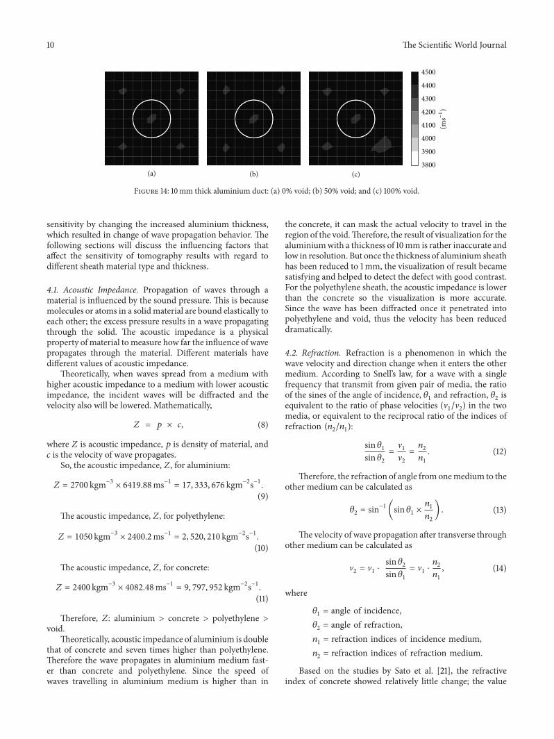
3.3.2. Effect of Aluminium Tendon Duct. Figures 7 and 14are the tomograms of concrete model containing 20 sensorsattached to four sides and simulated into 100 degrees offreedom. Tomograms in Figures 7(a), 7(b), and 7(c) have1mm thick aluminium tendon duct with 200mm diameteras shown with black colour in the figure. Tomogram inFigure 7(a) relates to the model with 0% void inside thealuminium tendon duct, tomogram in Figure 7(b) relatesto the model with 50% void inside the aluminium tendonduct, and tomogram in Figure 7(c) has 100% void insidethe aluminium tendon duct. The visualization of tomogramsin Figure 7 is acceptable. However, the other three tomo-grams which are tomogram in Figure 14(a), tomogram inFigure 14(b), and tomogram in Figure 14(c) have 10mm thickaluminium tendon duct with 200mm diameter as shownin white colour in three figures. It can be seen that besidetomogram in Figure 14(a), the visualization of tomograms inFigures 14(b) and 14(c) were unable to distinguish the size ofvoid.

4. Discussion

Throughout all the tomograms in this experiment, it isfound that the TTT is not applicable to detect void for500mm square concrete model that contains 10mm thickaluminium tendon duct. This was mainly due to the reduced


4000

3900

3800

4300

4200

4500

4400

4100 (ms−

1)

(a) (b) (c)

Figure 14: 10mm thick aluminium duct: (a) 0% void; (b) 50% void; and (c) 100% void.

sensitivity by changing the increased aluminium thickness,which resulted in change of wave propagation behavior. Thefollowing sections will discuss the influencing factors thataffect the sensitivity of tomography results with regard todifferent sheath material type and thickness.

4.1. Acoustic Impedance. Propagation of waves through amaterial is influenced by the sound pressure. This is becausemolecules or atoms in a solidmaterial are bound elastically toeach other; the excess pressure results in a wave propagatingthrough the solid. The acoustic impedance is a physicalproperty of material tomeasure how far the influence of wavepropagates through the material. Different materials havedifferent values of acoustic impedance.

Theoretically, when waves spread from a medium withhigher acoustic impedance to a medium with lower acousticimpedance, the incident waves will be diffracted and thevelocity also will be lowered. Mathematically,

𝑍 = 𝑝 × 𝑐, (8)

where 𝑍 is acoustic impedance, 𝑝 is density of material, and𝑐 is the velocity of wave propagates.

So, the acoustic impedance, 𝑍, for aluminium:

𝑍 = 2700 kgm−3 × 6419.88ms−1 = 17, 333, 676 kgm−2s−1.(9)

The acoustic impedance, 𝑍, for polyethylene:

𝑍 = 1050 kgm−3 × 2400.2ms−1 = 2, 520, 210 kgm−2s−1.(10)

The acoustic impedance, 𝑍, for concrete:

𝑍 = 2400 kgm−3 × 4082.48ms−1 = 9, 797, 952 kgm−2s−1.(11)

Therefore, 𝑍: aluminium > concrete > polyethylene >

void.Theoretically, acoustic impedance of aluminium is double

that of concrete and seven times higher than polyethylene.Therefore the wave propagates in aluminium medium fast-er than concrete and polyethylene. Since the speed ofwaves travelling in aluminium medium is higher than in

the concrete, it can mask the actual velocity to travel in theregion of the void.Therefore, the result of visualization for thealuminiumwith a thickness of 10mm is rather inaccurate andlow in resolution. But once the thickness of aluminium sheathhas been reduced to 1mm, the visualization of result becamesatisfying and helped to detect the defect with good contrast.For the polyethylene sheath, the acoustic impedance is lowerthan the concrete so the visualization is more accurate.Since the wave has been diffracted once it penetrated intopolyethylene and void, thus the velocity has been reduceddramatically.

4.2. Refraction. Refraction is a phenomenon in which thewave velocity and direction change when it enters the othermedium. According to Snell’s law, for a wave with a singlefrequency that transmit from given pair of media, the ratioof the sines of the angle of incidence, 𝜃

1

and refraction, 𝜃2

isequivalent to the ratio of phase velocities (V

1

/V2

) in the twomedia, or equivalent to the reciprocal ratio of the indices ofrefraction (𝑛

2

/𝑛1

):

sin 𝜃1

sin 𝜃2

=V1

V2

=𝑛2

𝑛1

. (12)

Therefore, the refraction of angle fromonemedium to theother medium can be calculated as

𝜃2

= sin−1 (sin 𝜃1

×𝑛1

𝑛2

) . (13)

The velocity of wave propagation after transverse throughother medium can be calculated as

V2

= V1

⋅sin 𝜃2

sin 𝜃1

= V1

⋅𝑛2

𝑛1

, (14)

where

𝜃1

= angle of incidence,𝜃2

= angle of refraction,𝑛1

= refraction indices of incidence medium,𝑛2

= refraction indices of refraction medium.

Based on the studies by Sato et al. [21], the refractiveindex of concrete showed relatively little change; the value


a week after concreting was 2.79, while that obtained fourteenmonths after concreting was 2.55. In this case, it is assumedthat the refractive index is 2.55. Generally, the refractiveindices of aluminium, polyethylene, and air are 1.44, 1.55, and1.00 relatively.

Figure 15 is an illustration of ray propagation fromconcrete to aluminium having a refraction factor (𝑛

2

/𝑛1

) of1.771. On the hand, Figure 16 refers to wave propagatingfrom concrete to polyethylene, the refraction factor (𝑛

2

/𝑛1

)is 1.645.It shows that the refraction factor for concrete-aluminium is higher than that of concrete-polyethylene.Thisexplainswhy thewave velocities of concretemodel containing10mm aluminium thick tendon duct are relatively fast atmore than 4500ms−1, resulting in that the void cannot beproperly visualized due to the masking effect.

4.3. Young’s Modulus and p-Wave Velocity of Material. Themechanical properties such as young’s modulus and p-wavevelocity of concrete and tendon duct have a big influence onspeed of wave propagation. Velocity of p-waves in homoge-neous, semi-infinite, elastic solids is defined as

𝐶𝑝

= √𝐸 (1 − 𝜎)

𝜌 (1 + 𝜎) (1 − 2𝜎), (15)

where 𝐶𝑝

is p-wave velocity, 𝐸 is Yong’s modulus of material,𝜌 is the density of material, and 𝜎 is the Poisson’s ratio ofmaterial. Commonly the Poisson’s ratio of aluminium andpolyethylene is 0.34 which has been used in simulations.Also, the Young’s modulus of aluminium and polyethyleneare 69GPa and 3.5GPa, while the density of aluminium andpolyethylene is 2700 and 1050 kg/m3, respectively, and wasalso inputted on simulations. By substituting the values ofPoisson’s ratio, Young modulus, and density of aluminiumand polyethylene into (12), it will give the p-wave velocityof aluminium and polyethylene as 6400ms−1 and 4000ms−1,respectively. Since p-wave can travel very fast on aluminium,therefor 10mm thick aluminium tendon duct could possiblymask the actual velocity of wave even though it is travelling inthe void. Since polyethylene will not cause acceleration to thewave propagation speed, 10mm thick polyethylene tendonduct will not affect the visualization of tomograms.

4.4. Transmission of Wave in Tendon Duct. It is consideredthat the tendon duct can be a medium for wave to travelthrough. It is already known that waves propagate faster inaluminium than concrete and polyethylene. A 10mm thickaluminium sheath is capable of acting as a pathway for thewave to travel as illustrated in Figure 17. The aluminiumtendon duct now has become the shortest path for thewaves to be propagated to its destination which are receiversensors. In this condition, the receiver sensor has detected thewave travel from tendon duct instead of its actual pathway.Therefore, regardless of the filling condition inside tendonduct, visualization by tomographywould not give remarkablydifferent between grouted and ungrouted tendon duct. Theset of travel times from the source to sensors x, y and z for1mm-thick and 10mm-thick aluminium tendon sheaths with

Incident wave

Refracted wave

Concrete

Aluminium

𝜃1

𝜃2

�1

�2

�2 = �1 × 1.771

𝜃2 = sin−1(sin𝜃1 × 1.771)

Figure 15: Refraction of wave from concrete medium to aluminiummedium.

Incident wave

Refracted wave

Concrete

Polyethylene

𝜃1

𝜃2

�1

�2

�2 = �1 × 1.645

𝜃2 = sin−1(sin𝜃1 × 1.645)

Figure 16: Refraction of wave from concrete medium to polyethy-lene medium.

Receiver node

Excitation node

Tendon duct

Concrete

Figure 17: Transmission of elastic wave from source to receiverthrough tendon duct.


100% void inside the tendon duct as illustrated in Figure 18were extracted and tabulated in Table 1. It is confirmed thatthe wave travel time in the concrete model with 10mmthick aluminium tendon sheath has been always faster thanconcrete model with 1mm thick aluminium tendon sheath,with the difference being approximately higher than 8.5%.

5. Quantification of Void

Figure 19 presents void quantification results of models sim-ulated with 100% void inside tendon duct, computed as voiddetection ratio against the type of tendon sheathmaterial.Theratio is calculated by proportioning the region with velocityless than 3900ms−1 as indicated by tomography result withthat of the actual modeled area. Three types of tendonsheaths were compared, namely, the 1mm aluminium, 1mmpolyethylene, and 10mm polyethylene. All the models weresimulated using 100 elements. In this figure, the ratio closestto 1.0 is considered the most accurate. Based on the results, itis understood that the most effective material in visualizationof void is 10mm thick polyethylene tendon sheath followedby 1mm thick polyethylene and 1mm thick aluminium. It isalso confirmed that the four-side sensor arrangement yieldedslightly better accuracy in detection than the two-side sensorarrangement.

Figure 20, on the other hand, presents the results of thevoid quantification comparison between models with 50%and 100% void, using different types of tendon sheaths. Allthe models were simulated using 100 elements. For the modelwith 1mm thick aluminium tendon sheath, void detectionratio is low for both 50% and 100% voided conditions. Also,quantification for 100% void is more accurate than that of50% void. For model with 1mm thick polyethylene sheath,detection accuracy for both void conditions is almost similar,which is approximately 0.6. For the case of 10mm thickpolyethylene sheath, quantification accuracy is slightly inexcess with ratio of 1.146 for 50% void, compared to 100% voidcondition, which is lower at 0.7.

The results of quantifying voids inside 10mm thickpolyethylene tendon sheath with different filling percentagesand sensor arrangements are given in Figure 21. The resultshows that for the model with 50% void inside 10mmpolyethylene tendon sheath and four-side sensor arrange-ment, the detection ratio is 0.8 by using 25 elements, whichshifts to approximately 1.15 when the number of elementswas increased to 100. This indicates that although detectionwas successful, estimation of the void area has been slightlyexcessive. Moreover, for the model with 10mm polyethylenetendon sheath and two-side sensor attachment, better accu-racy in size estimation was achieved with only 25 elementscompared to using the 100 elements. While for the modelof concrete with 10mm polyethylene and four-side sensorsarrangement, the quantification of void becomes better withincreasing the number of element to 100. Based on the resultspresented by the three cases, it can be confirmed that voiddetection and quantification by tomography reconstructiongives a minimum of 60% accuracy, which can be consideredas satisfactory.

Source

200 mm

Void

Aluminium tendon sheath

500mm

500mm

100mm

100mm

Sensor Sensor

Sensor “z”

“y”“x”

Figure 18: Illustration of location of sensors “𝑎”, “𝑥”, “𝑦”, and “𝑧”.

aluminium polyethylene polyethylene

2 sides of sensors attached

0.407 0.542 0.636

4 sides of sensors attached

0.509 0.636 0.722

00.10.20.30.40.50.60.70.8

Void

det

ectio

n ra

tio

1mm 1mm 10mm

Figure 19: Void detection ratio for models with two-side and four-side sensor arrangements.

6. Conclusions

Based on the study, conclusions can be made as follows.

(i) The visualization by tomography reconstruction tech-nique becomes better with increasing number ofsensors. Also placement of sensors on all four sidesof the concrete model improves the visualizationsignificantly. But, it is almost impossible to con-duct completely coverage tomography reconstructiontechnique on concrete structure, so it is important toknow how to interpret the tomogram with two sidesof transducers coverage.

(ii) Reducing the element/mesh size or increasing num-ber of elements/meshing did not necessarily improvethe visualization for void in tendon duct. In somecases, it led to confusion in results interpretation.

(iii) The material type and thickness of the sheath havean influence on accuracy of visualization, becauseof differences in the acoustic impedance and elastic


Table 1: Set of travel time from source to sensors at locations “𝑥”, “𝑦”, and “𝑧”.

Distance (mm)Travel time (ms)

Percentage different between 1mm and10mm thick aluminium (%)With 1mm thick

aluminiumWith 10mm thick

aluminium640.312 (source to sensor 𝑥) 0.153 0.141 8.511707.107 (source to sensor 𝑦) 0.173 0.159 8.805640.312 (source to sensor 𝑧) 0.153 0.141 8.511

0

0.2

0.4

0.6

0.8

1

1.2

Void

det

ectio

n ra

tio

aluminium polyethylene polyethylene

50% void

0.191 0.579 1.146

100% void

0.509 0.636 0.722

1mm 1mm 10mm

Figure 20: Void detection ratio for models with 50% void and 100%void.

25 elements100 elements

50% voidand 4 sides

100% voidand 2 sides

100% voidand 4 sides

0.755 0.764 0.6141.145 0.636 0.722

0

0.2

0.4

0.6

0.8

1

1.2

Void

det

ectio

n ra

tio

Figure 21: Ratio of detected void to actual void regarding the 25elements and 100 elements.

properties. This is demonstrated by the visualizationfor 10mm thick aluminium tendon sheath, whichis less accurate as compared with the 10mm thickpolyethylene.

(iv) It is important to conduct preliminary studies such asnumerical simulations on target structure before con-ducting the actual NDT on concrete structure.This isbecause the numerical simulations are considered to

be the early design stages of NDT to check whetherthe NDT technique is suitable to conduct to targetstructure.

Conflict of Interests

The authors declare that there is no conflict of interestsregarding the publication of this paper.

Acknowledgment

The authors acknowledge the support from University ofMalaya HIR Grant (UM.C/625/1/HIR/089).

References

[1] J. Martin, K. J. Broughton, A. Giannopolous, M. S. A. Hardy,and M. C. Forde, “Ultrasonic tomography of grouted ductpost-tensioned reinforced concrete bridge beams,” NDT & EInternational, vol. 34, no. 2, pp. 107–113, 2001.

[2] N. Alver, M. Tokai, Y. Nakai, and M. Ohtsu, “Identification ofimperfectly-grouted tendon-duct in Concrete by Sibie proce-dure,” in Proceedings of the European NDT Days, pp. 9–14, NDEfor Safety, Prague, Czech Republic, November 2007.

[3] M. Ohtsu and T. Watanabe, “Stack imaging of spectral ampli-tudes based on impact-echo for flaw detection,” NDT & EInternational, vol. 35, no. 3, pp. 189–196, 2002.

[4] N. Alver and M. Ohtsu, “BEM analysis of dynamic behaviorof concrete in impact-echo test,” Construction and BuildingMaterials, vol. 21, no. 3, pp. 519–526, 2007.

[5] K. Hoegh, L. Khazanovich, and H. T. Yu, “Ultrasonic tomog-raphy for evaluation of concrete pavements,” TransportationResearch Record, no. 2232, pp. 85–94, 2011.

[6] O. Buyukozturk, “Imaging of concrete structures,” NDT & EInternational, vol. 31, no. 4, pp. 233–243, 1998.

[7] K. J. Langenberg, K. Mayer, and R. Marklein, “Nondestructivetesting of concrete with electromagnetic and elastic waves:modeling and imaging,”Cement&Concrete Composites, vol. 28,no. 4, pp. 370–383, 2006.

[8] C. Rieck and B. Hillemeier, “Detecting voids inside ducts ofbonded steel tendons using impulse thermography,” in Proceed-ings of the International Symposium Non-Destructive Testing inCivil Engineering (NDT-CE ’03), Berlin, Germany, September2003.

[9] M. R. Clark, D. M. McCann, and M. C. Forde, “Applicationof infrared thermography to the non-destructive testing ofconcrete and masonry bridges,”NDT& E International, vol. 36,no. 4, pp. 265–275, 2003.


[10] D. G. Aggelis and T. Shiotani, “Repair evaluation of concretecracks using surface and through-transmission wave measure-ments,” Cement & Concrete Composites, vol. 29, no. 9, pp. 700–711, 2007.

[11] D. G. Aggelis and T. Shiotani, “Surface wave dispersion incement-based media: inclusion size effect,” NDT & E Interna-tional, vol. 41, no. 5, pp. 319–325, 2008.

[12] C. Cheng andM. Sansalone, “The impact-echo response of con-crete plates containing delaminations: numerical, experimentaland field studies,” Materials and Structures, vol. 26, no. 5, pp.274–285, 1993.

[13] T. Gudra and B. Stawiski, “Non-destructive strength characteri-zation of concrete using surface waves,”NDT& E International,vol. 33, no. 1, pp. 1–6, 2000.

[14] M. Ohtsu and N. Alver, “Development of non-contact SIBIEprocedure for identifying ungrouted tendon duct,” NDT & EInternational, vol. 42, no. 2, pp. 120–127, 2009.

[15] L. Vergara, R. Miralles, J. Gosalbez et al., “NDE ultrasonicmethods to characterise the porosity of mortar,” NDT & EInternational, vol. 34, no. 8, pp. 557–562, 2001.

[16] M. F. Kaplan, “The effects of age and water/cement ratio uponthe relation between ultrasonic pulse velocity and compressivestrength,”Magazine of Concrete Research, vol. 11, no. 32, pp. 85–92, 1959.

[17] D. A. Anderson and R. K. Seals, “Pulse velocity as a predictor of28-day and 90-day strength,” Journal of the American ConcreteInstitute, vol. 78, no. 2, pp. 116–122, 1981.

[18] D. G. Aggelis, N. Tsimpris, H. K. Chai, T. Shiotani, and Y.Kobayashi, “Numerical simulation of elastic waves for visual-ization of defects,” Construction and Building Materials, vol. 25,no. 4, pp. 1503–1512, 2011.

[19] H. K. Chai, S. Momoki, Y. Kobayashi, D. G. Aggelis, andT. Shiotani, “Tomographic reconstruction for concrete usingattenuation of ultrasound,” NDT & E International, vol. 44, no.2, pp. 206–215, 2011.

[20] S. Momoki, T. Shiotani, H. K. Chai, D. G. Aggelis, and Y.Kobayashi, “Large-scale evaluation of concrete repair by three-dimensional elastic-wave based visualization technique,” Struc-tural Health and Monitoring, vol. 12, no. 3, pp. 241–252, 2013.

[21] K. Sato, T. Manabe, J. Polivka, T. Ihara, Y. Kasashima, andK. Yamaki, “Measurement of the complex refractive index ofconcrete at 57.5 GHz,” IEEE Transactions on Antennas andPropagation, vol. 44, no. 1, pp. 35–40, 1996.

International Journal of

AerospaceEngineeringHindawi Publishing Corporationhttp://www.hindawi.com Volume 2014

RoboticsJournal of

Hindawi Publishing Corporationhttp://www.hindawi.com Volume 2014


Active and Passive Electronic Components

Control Scienceand Engineering

Journal of



RotatingMachinery


Hindawi Publishing Corporation http://www.hindawi.com

Journal ofEngineeringVolume 2014

Submit your manuscripts athttp://www.hindawi.com

VLSI Design



Shock and Vibration


Civil EngineeringAdvances in

Acoustics and VibrationAdvances in



Electrical and Computer Engineering

Journal of

Advances inOptoElectronics

Hindawi Publishing Corporation http://www.hindawi.com

Volume 2014

The Scientific World JournalHindawi Publishing Corporation http://www.hindawi.com Volume 2014

SensorsJournal of


Modelling & Simulation in EngineeringHindawi Publishing Corporation http://www.hindawi.com Volume 2014


Chemical EngineeringInternational Journal of Antennas and

Propagation




Navigation and Observation



DistributedSensor Networks


research article condition assessment of pc...

Documents