research article the use of response surface methodology...
TRANSCRIPT

Research ArticleThe Use of Response Surface Methodology to OptimizeParameter Adjustments in CNC Machine Tools
Shao-Hsien Chen,1 Wern-Dare Jehng,1 and Yen-Sheng Chen2
1 Department of Mechanical Engineering, National Chin-Yi University of Technology, No. 57, Section 2, Zhongshan Road,Taiping District, Taichung 41170, Taiwan
2Department of Automation, Lan Yang Institute of Technology, Taiwan
Correspondence should be addressed to Shao-Hsien Chen; [email protected]
Received 28 January 2014; Accepted 22 March 2014; Published 10 June 2014
Academic Editor: Her-Terng Yau
Copyright © 2014 Shao-Hsien Chen et al. This is an open access article distributed under the Creative Commons AttributionLicense, which permits unrestricted use, distribution, and reproduction in any medium, provided the original work is properlycited.
This paper mainly covers a research intended to improve the circular accuracy of CNC machine tools and the adjustment andanalysis of the main controller parameters applied to improve accuracy. In this study, controller analysis software was used todetect the adjustment status of the servo parameters of the feed axis. According to the FANUC parameter manual, the parameteraddress, frequency, responsemeasurements, and the one-fourth corner acceleration and decelerationmeasurements of themachinetools were adjusted. The experimental design (DOE) was adopted in this study for taking circular measurements and engaging inthe planning and selection of important parameter data. The Minitab R15 software was adopted to predict the experimental dataanalysis, while the seminormal probability map, Plato, and analysis of variance (ANOVA) were adopted to determine the impactsof the significant parameter factors and the interactions among them. Additionally, based on the response surface map and contourplot, the optimal values were obtained. In addition, comparison and verification were conducted through the Taguchi method,regression analysis to improvedmachining accuracy and efficiency.Theunadjusted errorwas 7.8𝜇m; through the regression analysismethod, the error was 5.8 𝜇m and through the Taguchi analysis method, the error was 6.4 𝜇m.
1. Introduction
In the age of technological advancement, machine tools haveplayed an essential role in automated production. Manualproduction simply cannot parallel the great processing man-ufacturing capacity and the processing accuracy of machinetools. Domestic and foreign machine tool factories aretherefore quite common. In terms of controller parameteradjustments, the trial and error method is usually adoptedto readily adjust the controller parameters, as breakthroughshave not yet been achieved. Hence, controller parameteradjustment remains an important issue for machine toolfactories. Moreover, as the controller is the core componentof a machine tool, without proper controller parameteradjustments, it is impossible to produce high-precision com-ponents.Therefore, the controller plays an essential role as faras machine tools are concerned.
Schulz et al. [1, 2] explained that high-speed cuttingcan improve productivity, while decreased cutting forces willresult in reduced thermal deformation, thus the good surfaceroughness and higher stability during cutting. Renton andElbestawi [3] targeted the high-speed servo control feedrate plan and servo loop control technique to shorten theprocessing time and path errors. Koren [4] mentioned thatspeed control and the position control loop are the two typesof control mainly adopted for machine tools, which mainlyinvolve the feed axis and speed feedback. Han et al. [5]used the look-ahead interpolation technique and high-speedprocessing algorithms to enhance the processing speed of theoriginal controller. However, the machine tool under high-speed processing inevitably led to processing accuracy errorsdue to the vibrations caused. Kim [6] compared the variousacceleration and deceleration and interpolation methods.Targeting poor accuracies during interpolation, a new rule
Hindawi Publishing CorporationMathematical Problems in EngineeringVolume 2014, Article ID 797091, 11 pageshttp://dx.doi.org/10.1155/2014/797091

2 Mathematical Problems in Engineering
was put forth: the acceleration and deceleration control wasapplied in the interpolator to ensure smoother processingand high-precision results. The well-known controllers fortool machines from home and abroad include FANUC,SIMENS, MITSUBISHI, and HEIDENHAIN. Among theleading brands, FANUC has taken the lead as far as controllerusage is concerned. The usage of the said brand is relativelyhigh among the domesticmachine tools.The FANUC 18i-MBcontroller functions are also in line with the high-speed andhigh-precision processing [7] 18i-MB controller’s functionalcharacteristics, which are needed for parameter adjustmentresearches.
2. The Parameters Affecting CircularTrajectory Accuracy
Prolonged use of machine tools in processing will inevitablylead to processing errors, which in turn affect the accuracy ofthe machine tools. Among them, (a) viscous motion errorsare due to poor lubrications of the bed and slide in contact,resulting in increased friction, hysteresis, and backlash errors.The phenomenon of quadrant vibration and the feed speedby a large extent have a positive relationship in which thefaster the feed speed is, the more obvious the protrusion ofthe cusps will be; (b) lost motion refers to the supportingpart of the ball screw and bearing being subject to the impactof elastic deformation, thus resulting in the excessive axialclearance of the bearing and insufficient rigidity, which inturn lead to elastic deformation and positive and negativeclearances that directly affect the arc cutting position and giverise to convexities and concavities; (c) the gain mismatch ofthe two-axis servo parameter positions when measuring thecircular trajectory will lead to one axis being ahead of theother, thus presenting an oval-shaped image; and (d) cuspsliding normally occurs at locations of quadrant changes,which leads to the production of repeated vibration noises. Athigh feed rates, the scope of vibration generation restrictedby vibrations will quickly disappear. At low feed rates,work pieces cannot undergo finishing processing, becauseof the emergence of cutting patterns during the cutting; (e)proportional errors will lead to tensile deformation, as shownin the circular measurement diagram. However, the amountof tensile deformation is usually not affected by the feed rateof the machine, possibly due to the overheating of screwsor changes in the compression and elongation of the opticallinear encoder; (f) vibration errors are probably related tomachine frequencies. Vibration causes the processing surfaceto form vibration patterns. Hence, it is necessary to enhancethe machine rigidity and reduce machine vibrations [8, 9].
It was found from the circular experiment that quadranterrors were produced due to transient phenomenon anderrors during the conversion of quadrants on the 𝑥𝑦 platformin the circular test. In general, a transient phenomenon isproduced due to the friction of the body system. After beingactivated, the motor’s servo system operated at a low speedproduces another transfer function which promotes themachine tool to shift from one transfer function to anotherat the circular speed of close to zero, thus the generation ofquadrant errors [10, 11].
Position Gain. Position gain adjustments affect program pathand actual path errors, and the error value is 𝐸. When theposition gains are the same, the higher the feed speed is, thegreater the amount of error will be. Consider
𝐸 =𝐹
𝐺. (1)
Velocity Gain. In terms of velocity loop gain related parameteradjustments, the data provided by the controller manufac-tures and various axial feed systems’ rigidity served as areference for the analysis and adjustment. When the velocityloop gain in the velocity loop was adjusted, the proportiongain and integral gain inside the velocity loop were affectedat the same time, as shown in Figures 1 and 2. For example,when the velocity loop gainwas enlarged, the proportion gainand integral gain were enlarged as well, while the proportiongain was deemed as the stiffness of the motor system, whichin turn determined the impact of the restoring force ofthe positive position errors. Thus, the higher proportiongain value accelerated the motor system responses, but italso resulted in the system’s instability due to impacts andoscillations.The integral gain was deemed as the static powermovements applied in the motor system. By adjusting theintegral gain, the position precision can be enhanced, butexcessive gain values will result in system instability andvibration [12].
3. Laboratory Equipment andExperimental Design
3.1. Laboratory Equipment. The laboratory equipmentmainly includes Takumi’s H10 gantry high-speed machinetool and the controller model FANUC 18i-MB. Theexperimental setup is as shown in Figure 2. Table 1 shows themachine specifications and models.
3.2. Experimental Design. In this study, the main processesinclude the following. In the first stage, the high-frequencyfiltering process was carried out mainly to reduce the impactof high-frequency responses on the machine precision; inthe second stage, the experimental parameter screening andanalysis were carried out mainly to analyze the weight of theCNC controller parameter impact on the circular trajectory;and in the third stage, the testing and analysis targetedthe parameters with higher weights of impact and thenthe optimization experiment was conducted. The Taguchianalysis results were also compared and discussed.
In terms of the experimental parameters in the circularmeasurement planning, the recommended values providedby the controller manufacturers served as a reference inthe parameter screening experiment. The main parametersas shown in Tables 5, 4, and 3 include the backlash com-pensation (1851), position gain (1825), velocity gain (2021),backlash accelerating rate (2018), and velocity loop gain ratiosduring cutting (2107). The important parameters affectingthe circular test were adjusted in the circular measurementimplementation. The direction of travel was in clockwise

Mathematical Problems in Engineering 3
Servo guide
Servo guide
Start
Programwindow
Graphicswindows
Sub-program transmission
Main program transmission
Access to date
Main memory for program
Use servo guideMade the program
MDI memory
MDI memory for testing
The servo guide autogenerated program
Use servo guideMade the program
The servo guide autogenerated program
NC
NC
Main memory for program
Figure 1: The controller process diagram.
Table 1: The machine specifications and models.
Stroke Spindle (built-in) The feed rate𝑥-axis 1020mm Motor 15/18.5 kW Cutting feed 1–20000mm/min
𝑦-axis 700mm Spindle taper BT-40 𝑥, 𝑦, and 𝑧-axesrapid feed 32/32/32m/min
𝑧-axis 500mm Spindle speed (continuous/30minutes of operation) 16000 rpm
Spindle noseto table 180–680mm
Machine tool
FANUC18i-MB
FANUCservoguide
Figure 2: The actual experimental machine: the H10 high-speedmachine tool.
rotation, the feed rate was 2000m/min, and the radius ofthe circle was 10mm when the measurement program wasimplemented. Through the circular trajectory diagram ofthe circular measurements, it was evident that during high-speed cutting, contour errors and overcuttingwere produced.Hence, the five important parameters were selected andthe software was used for the experimental plan (as shownin Table 2). According to the combination in the experi-mental plan, experimental measurements were conductedto measure the best conditions and find the best parametercombinations.
3.2.1. Analysis of Variance (ANOVA). Under the same signifi-cant standard𝛼, themethod used to detect whether or not themeans of 𝑘 number of population are equivalent is known asthe ANOVA. Table 1 shows the ANOVA table [13, 14].
The ANOVA steps are as follows.(1)The total variance is divided into experimental factor
variance and error variance; (2) each variance correspondingto the degree of freedom was determined; (3) the variance

4 Mathematical Problems in Engineering
40200
−20−40−60−80−100−120
Mon
Feb
. 14
16
:19
:05
2011
Mag
nitu
de (d
B)
10 20 50 100 200 500 1000
Frequency (Hz)
Frequency responseAxis-1: 10–1000Hz
(a)
0.00−45.00−90.00−135.00−180.00−225.00−270.00−315.00−360.00
10 20 50 100 200 500 1000Bode
mod
e pha
se (d
eg)
Frequency (Hz)
(b)
Figure 3: The 𝑥-axis frequency response measurement before filtering.
Table 2: The parameter addresses affecting circular measurements.
ParameterFunction
Backlashcompensation Position gain Velocity gain Backlash
accelerating rateVelocity loop gainratio during cutting
Parameterencoding 1851 1825 2021 2048 2107
Originalparameter
𝑥-axis 𝑦-axis 𝑥-axis 𝑦-axis 𝑥-axis 𝑦-axis 𝑥-axis 𝑦-axis 𝑥-axis 𝑦-axis0 5000 300 300 350 200
4.014003.0
12002.0
10001.08000.0600−1.0400−2.0200−3.0
0−4.0−200
Dra
w3
: FRE
Q (H
z)D
raw1
: TCM
D (%
)
Mon
Feb
. 14
16
:19
:05
2011
Frequency responseAxis-1: 10–1000Hz
Time (ms)0.00 1000.00 2000.00 3000.00 4000.00 5000.00
Figure 4: The 𝑥-axis torque command relative frequency diagrambefore filtering.
sum of square is divided by the degree of freedom into thevariance; (4) the 𝐹 statistics were obtained; and (5) when 𝐹 >
𝐹𝛼(]𝑅, ]𝐸), the impact of the𝑅 factor on the response value issignificant; when 𝐹 < 𝐹𝛼(]𝑅, ]𝐸), eth impact of the 𝑅 factoris not significant.
3.2.2. The Test Coefficient 𝑅2. The appropriateness of the
model can be determined by the test coefficient 𝑅2, which isdefined as
𝑅2=SS𝑅
SS𝑇
. (2)
SS𝑅is the progression sum of square, also known as the vari-
ance between populations:
SS𝑅
𝐾
∑
𝑖=1
𝑛𝑖
∑
𝑗=1
(𝑦𝑖− 𝑦 . . .)
2
=
𝑛𝑖
∑
𝑗=1
(𝑦𝑖− 𝑦 . . .)
2
, (3)
SS𝑇is the total sum of square, also known as the total vari-
ance:
SS𝑇
𝐾
∑
𝑖=1
𝑛𝑖
∑
𝑗=1
(𝑦𝑖𝑗− 𝑦 . . .)
2
,
SS𝑇= SS𝑅+ SS𝐸.
(4)
SS𝐸is the residual sum of square, also known as the variance
within the population. Consider
SS𝐸
𝐾
∑
𝑖=1
[
[
𝑛𝑖
∑
𝑗=1
(𝑦𝑖𝑗− 𝑦 . . .)
2]
]
. (5)
The 𝑅2 value is the ratio of the variance between pop-
ulations and the description of the total variance in theexperiment, which is the ratio explainable by the totalvariance of the experimental data.
3.2.3. The 𝐹 Value or 𝑡 Value Test . Whether or not the testedexperimental factors and their regression coefficients possesssignificance can be statistically tested through the 𝐹 value or𝑡 value. MS
𝐸is the residual sum of square, while MS
𝑅is the
mean sum of square. Consider
𝐹 =MS𝑅
MS𝐸
,
𝑡2= 𝐹.
(6)

Mathematical Problems in Engineering 5
40200
−20−40−60−80−100−120
Thu
Feb.
24
09
:38
:46
2011
Mag
nitu
de (d
B)
10 20 50 100 200 500 1000
Frequency (Hz)
Frequency responseAxis-1: 10–1000Hz
(a)
0.00−45.00−90.00−135.00−180.00−225.00−270.00−315.00−360.00
10 20 50 100 200 500 1000Bode
mod
e pha
se (d
eg)
Frequency (Hz)
(b)
Figure 5: The 𝑥-axis frequency response measurement after filtering.
4.014003.0
12002.0
10001.08000.0600−1.0400−2.0200−3.0
0−4.0−200
Dra
w3
: FRE
Q (H
z)D
raw1
: TCM
D (%
)
Frequency responseAxis-1: 10–1000Hz
Time (ms)0.00 1000.00 2000.00 3000.00 4000.00 5000.00
Thu
Feb.
24
09
:38
:46
2011
Figure 6: The 𝑥-axis torque command relative frequency diagramafter filtering.
Circ
le m
ode
R: 10.000X: −35.1426Y: 7.741801G: 500.0Z: 1.0
Fri J
un. 10
15
:03
:00
2011
+2.0 𝜇m
−2.0𝜇m
Figure 7: The circular errors of experiment 1 (error = 0.0071 𝜇).
4. Results and Discussion
4.1. The Frequency Response Measurement. Through the fre-quency response measurement, the resonance point of eachaxis of themachine toolwas found.Then, the filter parameterswere set to inhibit vibrations in high-frequency regions. Theset filter parameters were then transmitted to the machinetool model and the frequency responses were measured
+2.0 𝜇m
Circ
le m
ode
R: 10.000X: −10.0021Y: 0.002901G: 500.0Z: 1.0
Fri J
un. 10
17
:16
:15
2011
+2.0 𝜇m
Circ
le m
ode
X: −10.0021Y: 0.002901G: 500.0Z: 1.0
−2.0𝜇m
Figure 8: The circular errors of experiment 25 (error = 0.0083 𝜇).
1086420
2107
2021
1825
2048
1851
2.04
Term
(response is error, 𝛼 = 0.05)Pareto chart of the standardized effects
Standardized effect
Figure 9: The Plato of the first-order regression model in thecircular test.
again. The vibration-inhibiting waveform effectively inhib-ited machine vibrations during the high-speed processing(Figures 3 and 5).
4.1.1. Unfiltered Adjustment. For frequency response mea-surements of the 𝑥-axis before the filter adjustment, atfrequencies of 375Hz and 750Hz, the gain values were

6 Mathematical Problems in Engineering
Main effects plot for errorData means
1851
0 2
10
9
8
7
Mea
n
(a)
Main effects plot for errorData means
1825
3000 4000
10
9
8
7
Mea
n
(b)
2021
300 400
10
9
8
7
Mea
n
(c)
2048
50 350
10
9
8
7
Mea
n
(d)
2107
150 250
10
9
8
7
Mea
n
(e)
Figure 10: The main effects analysis diagram in the circular test.

Mathematical Problems in Engineering 7
210−1−2
99
90
50
10
1
Normal probability plot(%
)Residual plots for result
Residual
(a)
10.89.68.47.26.0
1
0
−1
−2
Resid
ual
Residual plots for resultVersus fits
Fitted value
(b)
1.20.80.40.0−0.4−0.8−1.2−1.6
8
6
4
2
0
Residual
Freq
uenc
y
Histogram
(c)
1
0
−1
−2
3230282624222018161412108642
Resid
ual
Versus order
Observation order
(d)
Figure 11: The residual analysis diagram in the circular test.
10 9
8 7
400380360340320300
250
225
200
175
150
1825, 3500Hold values
Result
Contour plot of result versus 2107, 2021
2107
<7
7-88-9
9-10>10
2021
Figure 12: The contour plot in the circular test.
Table 3: The filter adjustment.
HRV filter Center frequency(2113)
Bandwidth(2177)
Damping(2359)
HRV1 375 20 15HRV2 375 50 11
reduced to −339.5 db and −342.9 db, as shown in Figure 9.The reduction in the gain values was likely caused bymachineoil transmission or the operation of the motor fan spindle.Hence, from the measurement in the Bode diagram, instabil-ity was observed. As shown in Figure 10, the torque commandrelative frequency diagram can be used to switch the timedomain, indicating the feedback input waveforms in the Bodediagramand the corresponding frequencies (Figures 4 and 6).
4.1.2. High-Frequency Filtering Inhibits Vibrations. Throughvibration damping, the HRV1 filter frequency center param-eters (2113), bandwidth parameters (2177), damping parame-ters (2359), andHRV2 (2360), (2361), and (2362) adjustmentswere made, as listed in Table 3 [13]. As shown in Figure 11,the filtered frequency responses in the Bode diagram werecomparedwith the unfiltered one in Figure 9. It shows that noobvious gain value reductions were seen, thus indicating the

8 Mathematical Problems in Engineering
Data means
1851
0 2
Main effects plot for SN ratios
−17
−18
−19
−20
Mea
n of
SN
ratio
s
(a)
Data means
1825
3000 4000
Main effects plot for SN ratios
−17
−18
−19
−20
Mea
n of
SN
ratio
s(b)
2021
300 400
−17
−18
−19
−20
Mea
n of
SN
ratio
s
(c)
2048
50 350
−17
−18
−19
−20
Mea
n of
SN
ratio
s
(d)
2107
150 250
−17
−18
−19
−20
Mea
n of
SN
ratio
s
Signal-to-noise : smaller is better
(e)
Figure 13: The main effects analysis diagram in the circular test.
Mathematical Problems in Engineering 9
+2.0 𝜇m
−2.0𝜇mCi
rcle
mod
e
R: 10.000X: −35.142Y: 7.740201G: 500.0Z: 1.0
Fri J
un. 1
0 14
:58:
24 2
011
Draw 1
RGT: −1.5 : +6.3TOP: −2.3 : +1.9LFT: −2.5 : +4.6BTM: −3.0 : +1.5
(a) The accuracies of the original parameters
+2.0 𝜇m
−2.0𝜇m
Circ
le m
ode
R: 10.000
G: 500.0Z: 1.0
X: −10.0027Y: 0.002501
Fri J
un. 1
0 17
:19:
20 2
011
Draw 1
RGT: −2.2 : +3.6TOP: −2.4 : +2.5LFT: −2.5 : +2.6BTM: −2.8 : +2.0
(b) The adjusted accuracies of the regression analysisparameters
+2.0 𝜇m
−2.0𝜇m
Circ
le m
ode
R: 10.000X: −35.1426Y: 7.741801G: 500.0Z: 1.0
Fri J
un. 1
0 15
:44:
01 2
011
Draw 1
RGT: −2.0 : +4.4TOP: −2.9 : +1.9LFT: −2.4 : +3.2BTM: −2.5 : +2.1
(c) The adjusted accuracies of the Taguchi analysisparameters
Figure 14: The circular errors of experimental.
filter adjustments made to improve machine tool vibrationsproved to be effective [15].
4.2. The Measurement of Circular and CornerAcceleration and Deceleration
4.2.1. The Experimental Parameter Screening Analysis. Theparameter screening analysis was conducted for circularacceleration and deceleration, measurement, and data anal-ysis, as shown in Table 4 and DOE. The actual adjustedparameters on the 𝑥-axis and 𝑦-axis, through the circularmeasurements and circular trajectory diagram, clearly showthat, during high-speed cutting, the contour errors includedconvexity and overcutting.These phenomena produced enor-mous impacts on the surface roughness and contour ofthe work pieces during the high-speed cutting. Experi-mental measurements were then conducted based on the
combinations in the experimental planning, which furtherhelped determine the impacts of the five parameters oncircular errors (Figures 7 and 8).
The first-order regression model, Plato, in Figure 9 showsthe main effects of the control parameters or their inter-actions. The factors 1825, 2021, and 2107 represent pro-duced significant impacts. As Figure 9 shows, parameter 2107had the greatest impact on the circular accuracy, and theexperimental parameter was A2B2C1D2E2. The regressionmodel constructed underwent residual analysis to determinewhether or not the regression model was appropriate. Theresidual analysis and test in Figure 11 show that there wereno violations of the assumptions on the graphic changes, thusindicating that this configuration mode was in line with theassumption. As for the easiest method to determine whetheror not a stabile point is the maximum or minimum valueand decide the steep descending (ascending) direction, the

10 Mathematical Problems in Engineering
Table 4: The circular parameter setting of the machines.
Std.other
Runother
Centerpoint Blocks 1851 (𝐴) 1825 (𝐵) 2021 (𝐶) 2048 (𝐷) 2107 (𝐸) Error
20 1 1 1 2 4000 300 50 250 7.1333335 2 1 1 0 3000 400 50 150 9.4666674 3 1 1 2 4000 300 50 150 10.2666712 4 1 1 2 4000 300 350 150 10.566679 5 1 1 0 3000 300 350 150 11.6666717 6 1 1 0 3000 300 50 250 8.466667
23 34 1 1 0 4000 400 50 250 6.6333338 35 1 1 2 4000 400 50 150 8.26666727 36 1 1 0 4000 300 350 250 5.93333328 37 1 1 2 4000 300 350 250 5.766667
Table 5: Response table for means.
Level 1851 1825 2021 2048 21071 8.579 8.933 9.098 8.608 9.8852 8.362 8.008 7.844 8.333 7.056Delta 0.217 0.925 1.254 0.275 2.829Rank 5 3 2 4 1
model with a complete fit was used to draw contour plots andresponse surface maps in order to find the best points, whichis the best combination that optimizes the errors (shown inFigures 12 and 14).
4.2.2. The Regression Analysis Optimization Experiment. Allthe first-order standard factor combinations can fit into thefirst-order regression model as follows:
𝑦 = 𝛽0+ 𝛽1𝐴 + 𝛽
2𝐵 + 𝛽3𝐶 + 𝛽
4𝐷 + 𝛽
5𝐸 + 𝜀. (7)
𝐴 is the backslash compensation (1851), 𝐵 is the positiongain (1825), 𝐶 is the velocity gain (2021), 𝐷 is the backslashacceleration ratio (2048), and 𝐸 is the velocity loop gainduring cutting (2107), and engagement in first-order modeland lack-of-fit testing:
𝐻0: 𝑦 = 𝛽
0+ 𝛽1𝐴 + 𝛽
2𝐵 + 𝛽3𝐶 + 𝛽
4𝐷 + 𝛽
5𝐸
𝐻1: 𝑦 ̸= 𝛽
0+ 𝛽1𝐴 + 𝛽
2𝐵 + 𝛽3𝐶 + 𝛽
4𝐷 + 𝛽
5𝐸.
(8)
When the first-order model appropriateness testing was usedwith parameters 𝐴, 𝐵, 𝐶,𝐷, and 𝐸, the model’s 𝑃 value in thelack-of-fit testing was 0.81. A value greater than 𝛼 = 0.05 isthe rejected null hypothesis. From (9) it can be determinedthat the first-order lack-of-fit testing is 𝐻
0. The model’s
appropriateness, as determined by coefficient 𝑅2, is 0.8175. Avalue closer to 1 means the error is smaller. Consider
𝐹 =0.5787
0.9603= 0.602 > 𝐹
(0.05,26,4)(0.6) . (9)
When the first-order model appropriateness testing was usedwith parameters 𝐵, 𝐶, and 𝐸, the model’s 𝑃 value in the lack-of-fit testing was 0.09. A value greater than 𝛼 = 0.05 is
the rejected null hypothesis. From (10) it can be determinedthat the first-order lack-of-fit testing is 𝐻
1. The model’s
appropriateness, as determined by coefficient 𝑅2, is 0.8080.Consider
𝐹 =1.1747
0.5418= 2.168 < 𝐹
(0.05,28,4)(2.17) . (10)
Therefore, when the second-order model appropriatenesstesting was used, the model’s 𝑃 value in the lack-of-fit testingwas 0.852. A value greater than 𝛼 = 0.05 is the rejected nullhypothesis. From (11) it can be determined that the first-orderlack-of-fit is𝐻
1. The model’s appropriateness, as determined
by coefficient 𝑅2, is 0.8875. Consider
𝐹 =0.4873
0.9603= 0.507 < 𝐹
(0.05,16,4)(0.51) . (11)
The first-order optimized parameters were used to obtain theregression equation through experimentation:
𝑦 = 22.0479 − 0.108333𝐴 − 9.25000𝐸 − 04𝐵
− 0.0125417𝐶 − 9.16667𝑒 − 04𝐷 − 0.0282917𝐸.
(12)
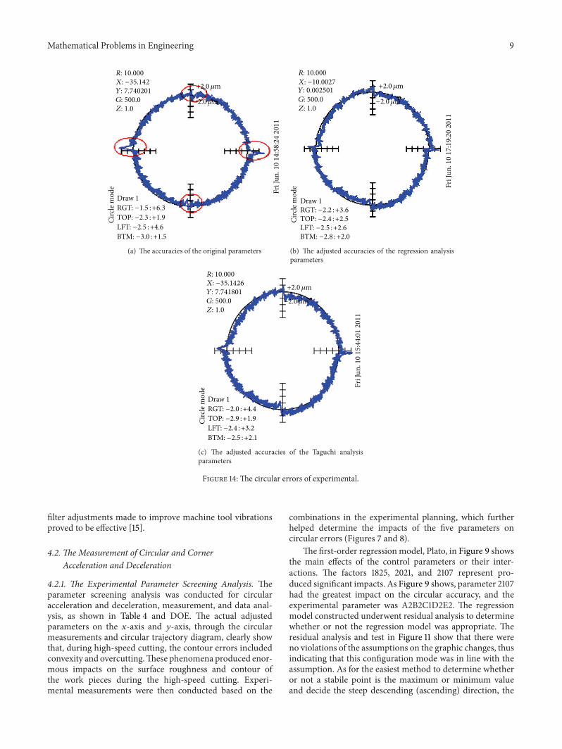
Based on the optimized parameters of 𝐴2𝐵2𝐶1𝐷2𝐸2, analy-sis and testing were conducted. The measured circular errorwas 0.0057mm, as shown in Figure 14. The circular accuracyhas reached optimized improvement.
4.2.3. The Taguchi Experimental Analysis. In the third stage,the regression equation of experimental parameter screen-ing and analysis was mainly used to select the importantparameters for optimization designing and testing. Thisexperimental test has a static 𝑆/𝑁 ratio of the “smaller thebetter.” The five levels of control factors, supplemented bythe L32 right angle table, were used for the analysis. Theoutputted data, based on the 𝑆/𝑁 ratio calculations and corre-sponding resolutions, is as shown in Figure 13.The optimizedparameter is 𝐴2𝐵2𝐶2𝐷2𝐸2, as shown in Table 5. Parameter2107 had the greatest impact on the circular accuracy andhad the same parameter as the regression analysis. Throughthe confirmation method in the experiment, the circularerror measured was 0.0064mm, while the circular accuracyachieved optimal accuracy using the Taguchi method [16].

Mathematical Problems in Engineering 11
4.2.4. A Comparison of the Regression Analysis and TaguchiAnalysis. In the first stage of this study, the regressionanalysis method was used to engage in parameter screeningapplications. In the second stage, the parameter optimiza-tion experiment mainly adopted the regression analysisand Taguchi method for comparison. The same findingwas obtained that the velocity loop gain ratio (2107) hadthe greatest error in the affected cusp during cutting. Theparameters of the two showed disparities in the analysis ofthe velocity gain (2021). Through the experiment, as shownin Figure 14, it was confirmed that the unadjusted error was7.8 𝜇m; through the regression analysis method, the error was5.8 𝜇m, and through the Taguchi analysis method, the errorwas 6.4 𝜇m, as shown in Figure 14.
5. Conclusion
The following conclusions can be drawn from this study.
(1) In this study, the regression equation method wasmainly used to engage in parameter screening, andthe empirical rules were avoided during the parame-ter screening. From the regression analysis method, itwas found that the velocity loop gain ratios, positiongains, and velocity gains had greater impacts on thecusps during cutting.
(2) In terms of optimized parameter adjustment, theregression analysis method and Taguchi methodwereadopted for comparison. Through the experiment, itwas confirmed that the unadjusted error was 7.8 𝜇m,through the regression analysis method, the error was5.8 𝜇m, and through the Taguchi analysis method,the error was 6.4 𝜇m. Hence, the regression analysismethod derived at higher accuracies.
(3) During the cutting, the higher the velocity loop gainratios, position gains, and velocity gains, the lowerthe relative cusp errors. However, the problem ofstructural resonance was likely.
Conflict of Interests
The authors declare that there is no conflict of interestsregarding the publication of this paper.
References
[1] H. Schulz and J. Scherer, “High-speed milling,” in Industrial &Production Engineering, 1989.
[2] H. Schulz and T. Moriwaki, “High-speed Machining,” CIRPAnnals: Manufacturing Technology, vol. 41, no. 2, pp. 637–643,1992.
[3] D. Renton and M. A. Elbestawi, “High speed servo controlof multi-axis machine tools,” International Journal of MachineTools and Manufacture, vol. 40, no. 4, pp. 539–559, 2000.
[4] Y. Koren, “Design of computer control for manufacturing sys-tems,” Journal of Engineering for Industry, vol. 101, no. 3, pp. 326–332, 1979.
[5] G.-C. Han, D.-I. Kim, H.-G. Kim, K. Nam, B.-K. Choi, and S.-K. Kim, “High speed machining algorithm for CNC machine
tools,” in Proceedings of the 25th Annual Conference of the IEEEIndustrial Electronics Society (IECON ’99), vol. 3, pp. 1493–1497,San Jose, Calif, USA, December 1999.
[6] D.-I. Kim, “Study on interpolation algorithms of CNCmachinetools,” in Proceedings of the Conference Record of the 1995 IEEEIndustry Applications 30th IAS Annual Meeting, pp. 1930–1937,October 1995.
[7] K.Ming-Sheng, “The FANUC controller vibrates suppresses theparameter adjustment,”Mechanical IndustryMagazine, vol. 275,2006.
[8] X.Mei,M.Tsutsumi, T. Yamazaki, andN. Sun, “Study of the fric-tion error for a high-speed high precision table,” InternationalJournal of Machine Tools and Manufacture, vol. 41, no. 10, pp.1405–1415, 2001.
[9] K. Erkorkmaz and Y. Altintas, “High speed CNC system design.Part III: High speed tracking and contouring control of feeddrives,” International Journal ofMachine Tools andManufacture,vol. 41, no. 11, pp. 1637–1658, 2001.
[10] S.-J. Huang and C.-C. Chen, “Application of self-tuning feed-forward and cross-coupling control in a retrofitted millingmachine,” International Journal of Machine Tools and Manufac-ture, vol. 35, no. 4, pp. 577–591, 1995.
[11] P. V. S. Suresh, P. Venkateswara Rao, and S. G. Deshmukh,“A genetic algorithmic approach for optimization of surfaceroughness prediction model,” International Journal of MachineTools and Manufacture, vol. 42, no. 6, pp. 675–680, 2002.
[12] FANUC, AC Servo Motor 𝛼i series, Parameter Manual.[13] E. Del Castillo, “Multiresponse process optimization via con-
strained confidence regions,” Journal of Quality Technology, vol.28, no. 1, pp. 61–70, 1996.
[14] W. E. Biles and J. J. Swain, “Response surfacemethod for experi-ential optimization of multi-responses process,” Industrial andEngineering Chemistry, vol. 13, no. 3, pp. 134–155, 2000.
[15] E. Del Castillo, D. C.Montgomery, andD. R.McCarville, “Mod-ified desirability functions for multiple response optimization,”Journal of Quality Technology, vol. 28, no. 3, pp. 337–345, 1996.
[16] J. A. Ghani, I. A. Choudhury, and H. H. Hassan, “Application ofTaguchimethod in the optimization of endmilling parameters,”Journal ofMaterials Processing Technology, vol. 145, no. 1, pp. 84–92, 2004.

Submit your manuscripts athttp://www.hindawi.com
Hindawi Publishing Corporationhttp://www.hindawi.com Volume 2014
MathematicsJournal of
Hindawi Publishing Corporationhttp://www.hindawi.com Volume 2014
Mathematical Problems in Engineering
Hindawi Publishing Corporationhttp://www.hindawi.com
Differential EquationsInternational Journal of
Volume 2014
Applied MathematicsJournal of
Hindawi Publishing Corporationhttp://www.hindawi.com Volume 2014
Probability and StatisticsHindawi Publishing Corporationhttp://www.hindawi.com Volume 2014
Journal of
Hindawi Publishing Corporationhttp://www.hindawi.com Volume 2014
Mathematical PhysicsAdvances in
Complex AnalysisJournal of
Hindawi Publishing Corporationhttp://www.hindawi.com Volume 2014
OptimizationJournal of
Hindawi Publishing Corporationhttp://www.hindawi.com Volume 2014
CombinatoricsHindawi Publishing Corporationhttp://www.hindawi.com Volume 2014
International Journal of
Hindawi Publishing Corporationhttp://www.hindawi.com Volume 2014
Operations ResearchAdvances in
Journal of
Hindawi Publishing Corporationhttp://www.hindawi.com Volume 2014
Function Spaces
Abstract and Applied AnalysisHindawi Publishing Corporationhttp://www.hindawi.com Volume 2014
International Journal of Mathematics and Mathematical Sciences
Hindawi Publishing Corporationhttp://www.hindawi.com Volume 2014
The Scientific World JournalHindawi Publishing Corporation http://www.hindawi.com Volume 2014
Hindawi Publishing Corporationhttp://www.hindawi.com Volume 2014
Algebra
Discrete Dynamics in Nature and Society
Hindawi Publishing Corporationhttp://www.hindawi.com Volume 2014
Hindawi Publishing Corporationhttp://www.hindawi.com Volume 2014
Decision SciencesAdvances in
Discrete MathematicsJournal of
Hindawi Publishing Corporationhttp://www.hindawi.com
Volume 2014 Hindawi Publishing Corporationhttp://www.hindawi.com Volume 2014
Stochastic AnalysisInternational Journal of