Chapter 3

Phonons; coupling to electrons

In this chapter we study the basic properties of ionic vibrations. These vibrations are welldescribed by harmonic oscillators and therefore we can employ the results from Sec. 1.4.1to achieve the second quantized form of the corresponding Hamiltonian. The quantizedvibrations are denoted phonons, a name pointing to the connection between sound wavesand lattice vibrations. Phonons play are fundamental role in our understanding of sound,specific heat, elasticity, and electrical resistivity of solids. And more surprising may bethe fact that the electron-phonon coupling is the cause of conventional superconductivity.In the following sections we shall study the three types of matter oscillation sketched inFig. 3.1. The ions will be treated using two models: the jellium model, where the ionsare represented by a smeared-out continuous positive background, and the lattice model,where the ions oscillate around their equilibrium positions forming a regular crystal lattice.

Since phonons basically are harmonic oscillators, they are bosons according to theresults of Sec. 1.4.1. Moreover, they naturally occur at finite temperature, so we willtherefore often need the thermal distribution function for bosons, the Bose-Einstein dis-tribution nB(ε) given in Eq. (1.127).

Figure 3.1: Three types of oscillations in metals. The grayscale represent the electrondensity and the dots the ions. (a) Slow ionic density oscillations in a static electron gas(ion plasma oscillations). The restoring force is the long range Coulomb interaction. (b)slow ion oscillations followed by the electron gas (sound waves, acoustic phonons). Therestoring force is the compressibility of the disturbed electron gas. (c) Fast electronicplasma oscillations in a static ionic lattice (electronic plasma oscillations). The restoringforce is the long range Coulomb interaction.

51

52 CHAPTER 3. PHONONS; COUPLING TO ELECTRONS

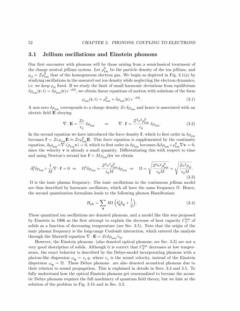
3.1 Jellium oscillations and Einstein phonons

Our first encounter with phonons will be those arising from a semiclassical treatment ofthe charge neutral jellium system. Let ρ0

ion be the particle density of the ion jellium, andρel = Zρ0

ion that of the homogeneous electron gas. We begin as depicted in Fig. 3.1(a) bystudying oscillations in the smeared out ion density while neglecting the electron dynamics,i.e. we keep ρel fixed. If we study the limit of small harmonic deviations from equilibriumδρion(r, t) = δρion(r)e−iΩt, we obtain linear equations of motion with solutions of the form

ρion(r, t) = ρ0ion + δρion(r) e−iΩt. (3.1)

A non-zero δρion corresponds to a charge density Ze δρion and hence is associated with anelectric field E obeying

∇ ·E =Ze

ε0δρion ⇒ ∇ · f =

Z2e2ρ0ion

ε0δρion. (3.2)

In the second equation we have introduced the force density f , which to first order in δρion

becomes f = ZeρionE ≈ Zeρ0ionE. This force equation is supplemented by the continuity

equation, ∂tρion+∇·(ρionv) = 0, which to first order in δρion becomes ∂tδρion+ρ0ion∇·v = 0,

since the velocity v is already a small quantity. Differentiating this with respect to timeand using Newton’s second law f = Mρion∂tv we obtain

∂2t δρion+

1M∇ · f = 0 ⇒ Ω2δρion =

Z2e2ρ0ion

ε0Mδρion ⇒ Ω =

√Z2e2ρ0

ion

ε0M=

√Ze2ρel

ε0M.

(3.3)Ω is the ionic plasma frequency. The ionic oscillations in the continuous jellium model

are thus described by harmonic oscillators, which all have the same frequency Ω. Hence,the second quantization formalism leads to the following phonon Hamiltonian:

Hph =∑q

~Ω(b†qbq +

12

). (3.4)

These quantized ion oscillations are denoted phonons, and a model like this was proposedby Einstein in 1906 as the first attempt to explain the decrease of heat capacity C ion

V ofsolids as a function of decreasing temperature (see Sec. 3.5). Note that the origin of theionic plasma frequency is the long-range Coulomb interaction, which entered the analysisthrough the Maxwell equation ∇ ·E = Zeδρion/ε0.

However, the Einstein phonons (also denoted optical phonons, see Sec. 3.3) are not avery good description of solids. Although it is correct that C ion

V decreases at low temper-ature, the exact behavior is described by the Debye-model incorporating phonons with aphoton-like dispersion ωq = vs q, where vs is the sound velocity, instead of the Einsteindispersion ωq = Ω. These Debye phonons are also denoted acoustical phonons due totheir relation to sound propagation. This is explained in details in Secs. 3.3 and 3.5. Tofully understand how the optical Einstein phonons get renormalized to become the acous-tic Debye phonons requires the full machinery of quantum field theory, but we hint at thesolution of the problem in Fig. 3.1b and in Sec. 3.2.

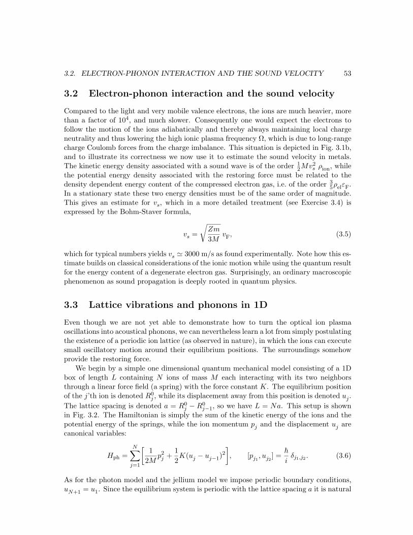
3.2. ELECTRON-PHONON INTERACTION AND THE SOUND VELOCITY 53

3.2 Electron-phonon interaction and the sound velocity

Compared to the light and very mobile valence electrons, the ions are much heavier, morethan a factor of 104, and much slower. Consequently one would expect the electrons tofollow the motion of the ions adiabatically and thereby always maintaining local chargeneutrality and thus lowering the high ionic plasma frequency Ω, which is due to long-rangecharge Coulomb forces from the charge imbalance. This situation is depicted in Fig. 3.1b,and to illustrate its correctness we now use it to estimate the sound velocity in metals.The kinetic energy density associated with a sound wave is of the order 1

2Mv2s ρion, while

the potential energy density associated with the restoring force must be related to thedensity dependent energy content of the compressed electron gas, i.e. of the order 3

5ρelεF.In a stationary state these two energy densities must be of the same order of magnitude.This gives an estimate for vs, which in a more detailed treatment (see Exercise 3.4) isexpressed by the Bohm-Staver formula,

vs =

√Zm

3MvF, (3.5)

which for typical numbers yields vs ' 3000 m/s as found experimentally. Note how this es-timate builds on classical considerations of the ionic motion while using the quantum resultfor the energy content of a degenerate electron gas. Surprisingly, an ordinary macroscopicphenomenon as sound propagation is deeply rooted in quantum physics.

3.3 Lattice vibrations and phonons in 1D

Even though we are not yet able to demonstrate how to turn the optical ion plasmaoscillations into acoustical phonons, we can nevertheless learn a lot from simply postulatingthe existence of a periodic ion lattice (as observed in nature), in which the ions can executesmall oscillatory motion around their equilibrium positions. The surroundings somehowprovide the restoring force.

We begin by a simple one dimensional quantum mechanical model consisting of a 1Dbox of length L containing N ions of mass M each interacting with its two neighborsthrough a linear force field (a spring) with the force constant K. The equilibrium positionof the j’th ion is denoted R0

j , while its displacement away from this position is denoted uj .The lattice spacing is denoted a = R0

j − R0j−1, so we have L = Na. This setup is shown

in Fig. 3.2. The Hamiltonian is simply the sum of the kinetic energy of the ions and thepotential energy of the springs, while the ion momentum pj and the displacement uj arecanonical variables:

Hph =N∑

j=1

[1

2Mp2

j +12K(uj − uj−1)

2

], [pj1

, uj2] =

~i

δj1,j2 . (3.6)

As for the photon model and the jellium model we impose periodic boundary conditions,uN+1 = u1. Since the equilibrium system is periodic with the lattice spacing a it is natural

54 CHAPTER 3. PHONONS; COUPLING TO ELECTRONS

!"#$

%& '( )* +, -. /0

1 23 4 5 1 23 4 6 1 23 1 23 7 6

8 3 4 5 8 3 4 6 8 3 8 3 7 6

9:9;9:9:9

<:<;<:<:<

Figure 3.2: A 1D lattice of ions with mass M , lattice constant a, and a nearest neighborlinear force coupling of strength K. The equilibrium positions shown in the top row aredenoted R0

j , while the displacements shown in the bottom row are denoted uj .

to solve the problem in k-space by performing a discrete Fourier transform. In analogywith electrons moving in a periodic lattice, also the present system of N ions forminga periodic lattice leads to a first Brillouin zone, FBZ, in reciprocal space. By Fouriertransformation the N ion coordinates becomes N wave vectors in FBZ:

FBZ =−π

a+ ∆k,−π

a+ 2∆k, . . . ,−π

a+ N∆k

, ∆k =

2π

L=

2π

a

1N

. (3.7)

The Fourier transforms of the conjugate variables are:

pj ≡ 1√N

∑

k∈FBZ

pkeikR0

j , uj ≡ 1√N

∑

k∈FBZ

ukeikR0

j , δR0

j ,0=

1N

∑

k∈FBZ

eikR0j ,

pk ≡ 1√N

N∑

j=1

pje−ikR0

j , uk ≡ 1√N

N∑

j=1

uje−ikR0

j , δk,0 =1N

N∑

j=1

e−ikR0j .

(3.8)By straight forward insertion of Eq. (3.8) into Eq. (3.6) we find

H =∑

k

[1

2Mpkp−k+

12Mω2

kuku−k

], ωk =

√K

M2∣∣∣sin ka

2

∣∣∣, [pk1, uk2

] =~iδk1,−k2 . (3.9)

This looks almost like the Hamiltonian for a set of harmonic oscillators except for someannoying details concerning k and −k. Note that while pj in real space is a nice Hermitianoperator, pk in k-space is not self-adjoint. In fact, the hermiticity of pj and the definition

of the Fourier transform lead to p†k = p−k. Although the commutator in Eq. (3.9) tells usthat uk and p−k form a pair of conjugate variables, we will not use this pair in analogywith x and p in Eq. (1.77) to form creation and annihilation operators. The reason isthat the Hamiltonian in the present case contains products like pkp−k and not p2

k as inthe original case. Instead we combine uk and pk in the definition of the annihilation and

3.3. LATTICE VIBRATIONS AND PHONONS IN 1D 55

Figure 3.3: The phonon dispersion relation for three different 1D lattices. (a) A systemwith lattice constant a and one ion of mass M1 (black disks) per unit cell. (b) As in (a)but now substituting every second ion of mass M1 with one of mass M2 (white disks)resulting in two ions per unit cell and a doubling of the lattice constant. To the left isshown the extended zone scheme, and to the right the reduced zone scheme. (c) As in (a)but now with the addition of mass M2 ions in between the mass M1 ions resulting in twoions per unit cell, but the same lattice constant as in (a).

creation operators bk and b†−k:

bk ≡ 1√2

(uk

`k+ i

pk

~/`k

), uk ≡ `k

1√2(b†−k + bk), `k =

√~

Mωk,

b†−k ≡ 1√2

(uk

`k− i

pk

~/`k

), pk ≡ ~

`k

i√2(b†−k − bk).

(3.10)

Note how both the oscillator frequency ωk = ω−k and the oscillator length `k = `−k

depends on the wavenumber k. Again by direct insertion it is readily verified that

Hph =∑

k

~ωk

(b†kbk +

12

), [bk1

, b†k2] = δk1,k2 . (3.11)

This is finally the canonical form of a Hamiltonian describing a set of independent har-monic oscillators in second quantization. The quantized oscillations are denoted phonons.

Their dispersion relation is shown in Fig. 3.3(a). It is seen from Eq. (3.9) that ωk−→k→0

√KM ak,

so our solution Eq. (3.11) does in fact bring about the acoustical phonons. The sound

velocity is found to be vs =√

KM a, so upon measuring the value of it, one can determine

the value of the free parameter K, the force constant in the model.If, as shown in Fig. 3.3(b), the unit cell is doubled to hold two ions, the concept of

phonon branches must be introduced. It is analogous to the Bloch bands for electrons.These came about as a consequence of breaking the translational invariance of the systemby introducing a periodic lattice. Now we break the discrete translational invariance givenby the lattice constant a. Instead the new lattice constant is 2a. Hence the original BZis halved in size and the original dispersion curve Fig. 3.3(a) is broken into sections. In

56 CHAPTER 3. PHONONS; COUPLING TO ELECTRONS

Figure 3.4: (a) An acoustical and (b) an optical phonon having the same wave length fora 1D system with two ions, • and , per unit cell. In the acoustical case the two types ofions oscillate in phase, while in the optical case they oscillate π radians out of phase.

the reduced zone scheme in Fig. 3.3(b) we of course find two branches, since no states canbe lost. The lower branch resembles the original dispersion so it corresponds to acousticphonons. The upper band never approaches zero energy, so to excite these phonons highenergies are required. In fact they can be excited by light, so they are known as opticalphonons. The origin of the energy difference between an acoustical and an optical phononat the same wave length is sketched in Fig. 3.4 for the case of a two-ion unit cell. Foracoustical phonons the size of the displacement of neighboring ions differs only slightlyand the sign of it is the same, whereas for optical phonons the sign of the displacementalternates between the two types of ions.

The generalization to p ions per unit cell is straight forward, and one finds the ap-pearance of 1 acoustic branch and (p-1) optical branches. The N appearing above, e.g.in Eq. (3.8), should be interpreted as the number of unit cells rather than the numberof ions, so we have Nion = pN . A branch index λ, analogous to the band index n forBloch electrons is introduced to label the different branches, and in the general case theHamiltonian Eq. (3.11) is changed into

Hph =∑

kλ

~ωkλ

(b†kλbkλ +

12

), [bk1λ1

, b†k2λ2] = δk1,k2

δλ1,λ2. (3.12)

3.4 Acoustical and optical phonons in 3D

The fundamental principles for constructing the second quantized phonon fields establishedfor the 1D case carries over to the 3D case almost unchanged. The most notable differenceis the appearance in 3D of polarization in analogy to what we have already seen for thephoton field. We treat the general case of any monatomic Bravais lattice. The ionicequilibrium positions are denoted R0

j and the displacements by u(R0j ) with components

uα(R0j ), α = x, y, z. The starting point of the analysis is a second order Taylor expansion

in uα(R0j ) of the potential energy U [u(R0

1), . . . ,u(R0N )],

U ≈ U0 +12

∑

R01R

02

∑

αβ

uα(R01)

∂2U

∂uα(R01) ∂uβ(R0

2)

∣∣∣∣∣u=0

uβ(R02). (3.13)

Note that nothing has been assumed about the range of the potential. It may very wellgo much beyond the nearest neighbor case studied in the 1D case. The central object in

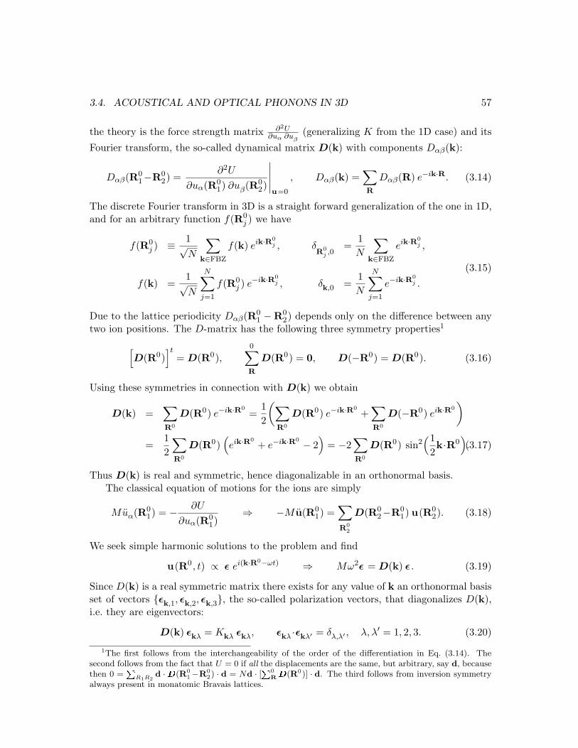
3.4. ACOUSTICAL AND OPTICAL PHONONS IN 3D 57

the theory is the force strength matrix ∂2U∂uα ∂uβ

(generalizing K from the 1D case) and its

Fourier transform, the so-called dynamical matrix D(k) with components Dαβ(k):

Dαβ(R01−R0

2) =∂2U

∂uα(R01) ∂uβ(R0

2)

∣∣∣∣∣u=0

, Dαβ(k) =∑

R

Dαβ(R) e−ik·R. (3.14)

The discrete Fourier transform in 3D is a straight forward generalization of the one in 1D,and for an arbitrary function f(R0

j ) we have

f(R0j ) ≡ 1√

N

∑

k∈FBZ

f(k) eik·R0j , δ

R0j ,0

=1N

∑

k∈FBZ

eik·R0j ,

f(k) =1√N

N∑

j=1

f(R0j ) e−ik·R0

j , δk,0 =1N

N∑

j=1

e−ik·R0j .

(3.15)

Due to the lattice periodicity Dαβ(R01 −R0

2) depends only on the difference between anytwo ion positions. The D-matrix has the following three symmetry properties1

[D(R0)

]t= D(R0),

0∑

R

D(R0) = 0, D(−R0) = D(R0). (3.16)

Using these symmetries in connection with D(k) we obtain

D(k) =∑

R0

D(R0) e−ik·R0=

12

(∑

R0

D(R0) e−ik·R0+

∑

R0

D(−R0) eik·R0

)

=12

∑

R0

D(R0)(eik·R0

+ e−ik·R0 − 2)

= −2∑

R0

D(R0) sin2(1

2k·R0

).(3.17)

Thus D(k) is real and symmetric, hence diagonalizable in an orthonormal basis.The classical equation of motions for the ions are simply

Muα(R01) = − ∂U

∂uα(R01)

⇒ −M u(R01) =

∑

R02

D(R02−R0

1) u(R02). (3.18)

We seek simple harmonic solutions to the problem and find

u(R0 , t) ∝ ε ei(k·R0−ωt) ⇒ Mω2ε = D(k) ε . (3.19)

Since D(k) is a real symmetric matrix there exists for any value of k an orthonormal basisset of vectors εk,1, εk,2, εk,3, the so-called polarization vectors, that diagonalizes D(k),i.e. they are eigenvectors:

D(k) εkλ = Kkλ εkλ, εkλ ·εkλ′ = δλ,λ′ , λ, λ′ = 1, 2, 3. (3.20)

1The first follows from the interchangeability of the order of the differentiation in Eq. (3.14). Thesecond follows from the fact that U = 0 if all the displacements are the same, but arbitrary, say d, becausethen 0 =

PR1R2

d ·D(R01−R0

2) · d = Nd · [P0RD(R0)] · d. The third follows from inversion symmetry

always present in monatomic Bravais lattices.

58 CHAPTER 3. PHONONS; COUPLING TO ELECTRONS

Figure 3.5: (a) Three examples of polarization in phonon modes: transverse, longitudinaland general. (b) A generic phonon spectrum for a system with 3 ions in the unit cell. The9 modes divides into 3 acoustical and 6 optical modes.

We have now found the classical eigenmodes ukλ of the 3D lattice vibrations characterizedby the wavevector k and the polarization vector εkλ:

Mω2εkλ = Kkλεkλ ⇒ ukλ(R0 , t) = εkλ ei(k·R0−ωkλt), ωkλ ≡√

Kkλ

M. (3.21)

Using as in Eq. (3.10) the now familiar second quantization procedure of harmonic oscil-lators we obtain

ukλ ≡ `kλ1√2

(b†−k,λ + bk,λ

)εkλ, `kλ ≡

√~

Mωkλ

, (3.22)

Hph =∑

kλ

~ωkλ

(b†kλbkλ +

12

), [bkλ, b†k′λ′ ] = δk,k′ δλ,λ′ . (3.23)

Now, what about acoustical and optical phonons in 3D? It is clear from Eq. (3.17)that D(k) ∝ k2 for k → 0, so the same holds true for its eigenvalues Kkλ. The dispersionrelation in Eq. (3.19) therefore becomes ωkλ = vλ(θk, φk) k, which describes an acousticalphonon with a sound velocity vλ(θk, φk) in general depending on both the direction of kand the polarization λ. As in 1D the number of ions in the unit cell can be augmented from1 to p. In that case it can be shown that of the resulting 3p modes 3 are acoustical and3(p−1) optical modes. The acoustical modes are appearing because it is always possible toconstruct modes where all the ions have been given nearly the same displacement resultingin an arbitrarily low energy cost associated with such a deformation of the lattice. InFig. 3.5 is shown the phonon modes for a unit cell with three ions.

A 3D lattice with N unit cells each containing p ions, each of which can oscillate in3 directions, is described by 3pN modes. In terms of phonon modes we end up with 3pso-called phonon branches ωkλ, which for each branch index λ are defined in N discretepoints in k-space. Thus in 3D the index λ contains information on both which polarizationand which of the acoustical or optical modes we are dealing with.

3.5. THE SPECIFIC HEAT OF SOLIDS IN THE DEBYE MODEL 59

3.5 The specific heat of solids in the Debye model

Debye’s phonon model is a simple model, which describes the temperature dependence ofthe heat capacitance CV = ∂E

∂T of solids exceedingly well, although it contains just onematerial dependent free parameter. The phonon spectrum Fig. 3.5(b) in the reduced zonescheme has 3p branches. In Fig. 3.6(a) is shown the acoustic and optical phonon branch inthe extended zone scheme for a 1D chain with two ions per unit cell. Note how the opticalbranch appears as an extension of the acoustical branch. In d dimensions a reasonableaverage of the spectrum can be obtained by representing all the phonon branches in thereduced zone scheme with d acoustical branches in the extended zone scheme, each with alinear dispersion relation ωkλ = vλk. Furthermore, since we will use the model to calculatethe specific heat by averaging over all modes, we can even employ a suitable average vD

out the polarization dependent velocities vλ and use the same linear dispersion relationfor all acoustical branches,

ωkλ ≡ vDk ⇒ ε = ~vD k. (3.24)

Even though we have deformed the phonon spectrum we may not change the number ofphonon modes. In the 3D Debye model we have 3Nion modes, in the form of 3 acousticbranches each with Nion allowed wavevectors, where Nion is the number of ions in thelattice. Since we are using periodic boundary conditions the counting of the allowedphonon wavevectors is equivalent to that of Sec. 2.1.2 for plane wave electron states, i.e.Nion = [V/(2π)3]×[volume in k-space]. Since the Debye spectrum Eq. (3.24) is isotropicin k-space, the Debye phonon modes must occupy a sphere in this space, i.e. all modeswith |k| < kD, where kD is denoted the Debye wave number determined by

Nion =V

(2π)343π k3

D. (3.25)

Inserting kD into Eq. (3.24) yields the characteristic Debye energy, ~ωD and hence thecharacteristic Debye temperature TD:

~ωD ≡ kBTD ≡ ~vD kD ⇒ 6π2 Nion (~vD)3 = V (kBTD)3. (3.26)

Continuing the analogy with the electron case the density of phonon states Dph(ε) is foundby combining Eq. (3.24) and Eq. (3.25) and multiplying by 3 for the number of acousticbranches,

Nion(ε) =V

6π2

1(~vD)3

ε3 ⇒ Dph(ε) = 3dNion(ε)

dε=

V2π2

1(~vD)3

ε2, 0 < ε < kBTD.

(3.27)The energy Eion(T ) of the vibrating lattice is now easily computed using the Bose-Einsteindistribution function nB(ε) Eq. (1.127) for the bosonic phonons:

Eion(T ) =∫ kBTD

0dε εDph(ε)nB(ε) =

V2π2

3(~vD)3

∫ kBTD

0dε

ε3

eβε − 1. (3.28)

60 CHAPTER 3. PHONONS; COUPLING TO ELECTRONS

! " # $ % & ' ( # )

**** *

* * * *

* ***

** *

* * * * *

* * ** *

*** *

* * *

* * * * * * ** ***** **

+ , - + . -/ 0

11 23

4 1 23

Figure 3.6: (a) The linear Debye approximation to the phonon spectrum with the Debyewave vector kD shown. (b) Comparison between experiment and the Debye model of heatcapacitance applied for lead, silver, aluminum, and diamond.

It is now straight forward to obtain C ionV from Eq. (3.28) by differentiation:

C ionV (T ) =

∂Eion

∂T= 9NionkB

( T

TD

)3∫ TD/T

0dx

x4 ex

(ex − 1)2, (3.29)

where the integrand is rendered dimensionless by introducing TD from Eq. (3.26). Notethat TD is the only free parameter in the Debye model of heat capacitance; vD droppedout of the calculation. Note also how the model reproduces the classical Dulong-Petitvalue in the high temperature limit, where all oscillators are thermally excited. In the lowtemperature limits the oscillators “freeze out” and the heat capacitance drops as T 3,

C ionV (T ) −→

T¿TD

12π4

5NionkB

( T

TD

)3, C ion

V (T ) −→TÀTD

3NionkB. (3.30)

In Fig. 3.6(b) the Debye model is compared to experiment. A remarkable agreementis obtained over the wide temperature range from 10 K to 1000 K after fitting TD for eachof the widely different materials lead, aluminum, silver and diamond.

We end this section by a historical remark. The very first published application ofquantum theory to a condensed matter problem was in fact Einstein’s work from 1906,reproduced in Fig. 3.7(a), explaining the main features of Weber’s 1875 measurements ondiamond. In analogy with Planck’s quantization of the oscillators related to the blackbody radiation, Einstein quantized the oscillators corresponding to the lattice vibrations,assuming that all oscillators had the same frequency ωE . So instead of Eq. (3.27), Einsteinemployed the much simpler DE

ion(ε) = δ(ε− ~ωE), which immediately leads to

C ion,EV (T ) = 3NionkB

(TE

T

)2 eTE/T

(eTE/T − 1)2, TE ≡ ~ωE/kB. (3.31)

While this theory also gives the classical result 3NionkB in the high temperature limit,it exaggerates the decrease of C ion

V at low temperatures by predicting an exponentialsuppression. In Fig. 3.7(b) is shown a comparison of Debye’s and Einstein’s models.Nowadays, Einstein’s formula is still in use, since it provides a fairly accurate descriptionof the optical phonons which in many cases have a reasonably flat dispersion relation.

3.6. ELECTRON-PHONON INTERACTION IN THE LATTICE MODEL 61

Figure 3.7: (a) The first application of quantum theory to condensed matter physics.Einstein’s 1906 theory of heat capacitance of solids. The theory is compared to Weber’s1875 measurements on diamond. (b) A comparison between Debye’s and Einstein’s model.

3.6 Electron-phonon interaction in the lattice model

In Chap. 2 we mentioned that in the lattice model the electron-ion interaction splits intwo terms, one arising from the static lattice and the other from the ionic vibrations,Vel−ion = Vel−latt +Vel−ph. The former has already been dealt with in the HBloch, so in thissection the task is to derive the explicit second quantized form of the latter. Regardingthe basis states for the combined electron and phonon system we are now in the situationdiscussed in Sec. 1.4.5. We will simply use the product states given in Eq. (1.108).

Our point of departure is the simple expression for the Coulomb energy of an electrondensity in the electric potential Vion(r−Rj) of an ion placed at the position Rj ,

Vel−ion =∫

dr (−e)ρel(r)N∑

j=1

Vion(r−Rj). (3.32)

As before the actual ion coordinates are given by Rj = R0j + uj , where R0

j are the ionicequilibrium positions, i.e. the static periodic lattice, and where uj denotes the latticevibrations. The respective contributions from these two sets of coordinates are separatedby a Taylor expansion, Vion(r −Rj) ≈ Vion(r −R0

j ) −∇rVion(r −R0j ) · uj , note the sign

of the second term, and we obtain

Vel−ion =∫

dr (−e)ρel(r)N∑

j=1

Vion(r−R0j )−

∫dr (−e)ρel(r)

N∑

j=1

∇rVion(r−R0j ) ·uj . (3.33)

The first term is the one entering HBloch in Eq. (2.6), while the second is the electron-phonon interaction, also sketched in Fig. 3.8,

Vel−ph =∫

dr ρel(r)∑

j

e uj · ∇rVion(r−R0j )

. (3.34)

Vel−ph is readily defined in real space, but a lot easier to use in k-space, so we will proceed

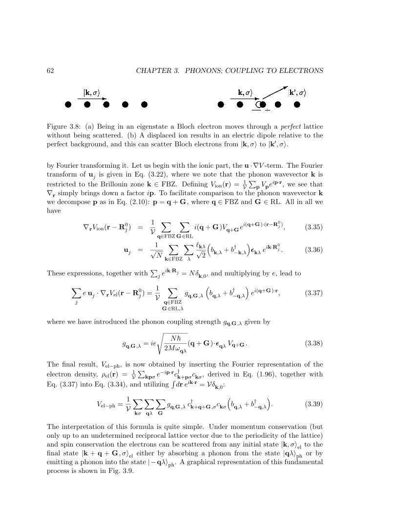
62 CHAPTER 3. PHONONS; COUPLING TO ELECTRONS

Figure 3.8: (a) Being in an eigenstate a Bloch electron moves through a perfect latticewithout being scattered. (b) A displaced ion results in an electric dipole relative to theperfect background, and this can scatter Bloch electrons from |k, σ〉 to |k′, σ〉.

by Fourier transforming it. Let us begin with the ionic part, the u ·∇V -term. The Fouriertransform of uj is given in Eq. (3.22), where we note that the phonon wavevector k isrestricted to the Brillouin zone k ∈ FBZ. Defining Vion(r) = 1

V∑

p Vpeip·r, we see that∇r simply brings down a factor ip. To facilitate comparison to the phonon wavevector kwe decompose p as in Eq. (2.10): p = q + G , where q ∈ FBZ and G ∈ RL. All in all wehave

∇rVion(r−R0j ) =

1V

∑

q∈FBZ

∑

G∈RL

i(q + G)Vq+Gei(q+G )·(r−R0j ), (3.35)

uj =1√N

∑

k∈FBZ

∑

λ

`kλ√2

(bk,λ + b†−k,λ

)εkλ eik·R0

j . (3.36)

These expressions, together with∑

j eik·Rj = Nδk,0, and multiplying by e, lead to

∑

j

e uj · ∇rVel(r−R0j ) =

1V

∑

q∈FBZ

G∈RL,λ

gq,G ,λ

(bq,λ + b†−q,λ

)ei(q+G )·r, (3.37)

where we have introduced the phonon coupling strength gq,G ,λ given by

gq,G ,λ = ie

√N~

2Mωqλ

(q + G)·εqλ Vq+G . (3.38)

The final result, Vel−ph, is now obtained by inserting the Fourier representation of theelectron density, ρel(r) = 1

V∑

kpσ e−ip·rc†k+pσckσ, derived in Eq. (1.96), together withEq. (3.37) into Eq. (3.34), and utilizing

∫dr eik·r = Vδk,0:

Vel−ph =1V

∑

kσ

∑

qλ

∑

G

gq,G ,λ c†k+q+G ,σckσ

(bq,λ + b†−q,λ

). (3.39)

The interpretation of this formula is quite simple. Under momentum conservation (butonly up to an undetermined reciprocal lattice vector due to the periodicity of the lattice)and spin conservation the electrons can be scattered from any initial state |k, σ〉el to thefinal state |k + q + G , σ〉el either by absorbing a phonon from the state |qλ〉ph or byemitting a phonon into the state |−qλ〉ph. A graphical representation of this fundamentalprocess is shown in Fig. 3.9.

3.7. ELECTRON-PHONON INTERACTION IN THE JELLIUM MODEL 63

Figure 3.9: A graphical representation of the fundamental electron-phonon coupling. Theelectron states are represented by the straight lines, the phonon states by curly spring-likelines, and the coupling strength by a dot. To the left the electron is scattered by absorbinga phonon, to the right by emitting a phonon.

The normal processes, i.e. processes where per definition G = 0, often tend to dominateover the so-called umklapp processes, where G 6= 0, so in the following we shall completelyneglect the latter.2 Moreover, we shall treat only isotropic media, where εqλ is eitherparallel to or perpendicular to q, i.e. q·εqλ in gq,G=0,λ is only non-zero for longitudinallypolarized phonons. So in the Isotropic case for Normal phonon processes we have

V INel−ph =

1V

∑

kσ

∑

qλl

gq,λlc†k+q,σckσ

(bq,λl

+ b†−q,λl

). (3.40)

Finally, the most significant physics of the electron-phonon coupling can often be extractedfrom considering just the acoustical modes. Due to their low energies they are excitedsignificantly more than the high energy optical phonons at temperatures lower than theDebye temperature. Thus in the Isotropic case for Normal Acoustical phonon processesonly the longitudinal acoustical branch enters and we have

V INAel−ph =

1V

∑

kσ

∑q

gq c†k+q,σckσ

(bq + b†−q

). (3.41)

If we for ions with charge +Ze approximate Vq by a Yukawa potential, Vq = Zeε0

1q2+k2

s(see

Exercise 1.5), the explicit form of the coupling constant gq is particularly simple:

gq = iZe2

ε0

q

q2 + k2s

√N~

2Mωq. (3.42)

3.7 Electron-phonon interaction in the jellium model

Finally, we return to the case of Einstein phonons in the jellium model treated in Sec. 3.1.The electron-phonon interaction in this case is derived in analogy with the that of normal

2There are mainly two reasons why the umklapp processes often can be neglected: (1) Vq+G is small

due to the 1/(q + G)2 dependence, and (2) At low temperatures the phase space available for umklappprocesses is small.

64 CHAPTER 3. PHONONS; COUPLING TO ELECTRONS

lattice phonons in the isotropic case, Eq. (3.41). If we as in Sec. 3.1 neglect the weakdispersion of the Einstein phonons and simply assume that they all vibrate with the ionplasma frequency Ω of Eq. (3.3), the result for N vibrating ions in the volume V is

V jelel−ph =

1V

∑

kσ

∑q

gjelq c†k+q,σckσ

(bq + b†−q

), (3.43)

with

gjelq = i

Ze2

ε0

1q

√N~

2MΩ. (3.44)

3.8 Summary and outlook

In this chapter we have derived the second quantized form of the Hamiltonian of theisolated phonon system and the electron-phonon coupling. The solution of the phononproblem actually constitutes our first solution of a real interacting many-particle system,each ion is coupled to its neighbors. Also the treatment of the electron-phonon couplingmarks an important step forward: here we dealt for the first time with the couplingbetween to different kinds of particles, electrons and phonons.

The electron-phonon coupling is a very important mechanism in condensed mattersystems. It is the cause of a large part of electrical resistivity in metals and semiconductors,and it also plays a major role in studies of heat transport. In Exercise 3.1 and Exercise 3.2give a first hint at how the electron-phonon coupling leads to a scattering or relaxationtime for electrons.

We shall return to the electron-phonon coupling in Chap. 16, and there see the firsthint of the remarkable interplay between electrons and phonons that lies at the heart of theunderstanding of conventional superconductivity. The very successful microscopic theoryof superconductivity, the so-called BCS theory, is based on the electron-phonon scattering,even the simple form given in Eqs. (3.41) and (3.42) suffices to cause superconductivity.

Chapter 16

Green’s functions and phonons

In this chapter we develop and apply the Green’s function technique for free phonons andfor the electron-phonon interaction. The point of departure is the second quantizationformulation of the phonon problem presented in Chap. 3, in particular the bosonic phononcreation and annihilation operators b†−q,λ and bq,λ introduced in Eqs. (3.10) and (3.22)and appearing in the jellium phonon Hamiltonian Eq. (3.4) and in the lattice phononHamiltonian Eq. (3.23).

We first define and study the Green’s functions for free phonons in both the jelliummodel and the lattice model. Then we apply the Green’s function technique to the electron-phonon interaction problem. We derive the one-electron Green’s function in the presenceof both the electron-electron and the electron-phonon interaction. We also show how thehigh frequency Einstein phonons in the free-phonon jellium model become renormalizedand become the usual low-frequency acoustic phonons once the electron-phonon interactionis taken into account. Finally, we prove the existence of the so-called Cooper instability ofthe electron gas, the phonon-induced instability which is the origin of superconductivity.

16.1 The Green’s function for free phonons

It follows from all the Hamiltonians describing electron-phonon interactions, e.g. HINAel−ph

in Eq. (3.41) and H jelel−ph in Eq. (3.43), that the relevant phonon operators to consider are

not the individual phonon creation and annihilation operators, but rather the operatorsAqλ and A†qλ defined as

Aqλ ≡(bqλ + b†−qλ

), A†qλ ≡

(b†qλ + b−qλ

)= A−qλ. (16.1)

The phonon operator Aqλ can be interpreted as removing momentum q from the phononsystem either by annihilating a phonon with momentum q or by creating one with mo-mentum −q. With these prerequisites the non-interacting phonons are described by Hph

and the electron-phonon interaction by Hel−ph as follows:

Hph =∑

qλ

Ωqλ

(b†qλbqλ +

12

), Hel−ph =

1V

∑

kσ

∑

qλ

gqλ c†k+q,σckσ Aqλ. (16.2)

275

276 CHAPTER 16. GREEN’S FUNCTIONS AND PHONONS

Since Hph does not depend on time, we can in accordance with Eq. (10.5) define thephonon operators Aqλ(τ) in the imaginary time interaction picture1

Aqλ(τ) ≡ eτHph Aqλ e−τHph . (16.3)

With this imaginary-time boson operator we can follow Eq. (10.17) and introduce thebosonic Matsubara Green’s function D0

λ(q, τ) for free phonons,

D0λ(q, τ) ≡ −⟨

Tτ Aqλ(τ)A†qλ(0)⟩0

= −⟨Tτ Aqλ(τ)A−qλ(0)

⟩0, (16.4)

where Tτ is the bosonic time ordering operator defined in Eq. (10.18) with a plus-sign.The frequency representation of the free phonon Green’s function follows by applyingEq. (10.25),

D0λ(q, iqn) ≡

∫ β

0dτ eiqnτ D0

λ(q, τ), ωn = 2nπ/β. (16.5)

The specific forms forD0λ(q, τ) andD0

λ(q, iqn) are found using the boson results of Sec. 10.3.1with the substitutions (ν, εν , cν) → (qλ,Ωqλ, bqλ). In the imaginary time domain we find

D0λ(q, τ) =

−[nB(Ωqλ) + 1

]e−Ωqλτ − nB(Ωqλ) eΩqλτ , for τ > 0,

−nB(Ωqλ) e−Ωqλτ − [nB(Ωqλ) + 1

]eΩqλτ , for τ < 0,

(16.6)

while in the frequency domain we obtain

D0λ(q, iqn) =

1iqn − Ωqλ

− 1iqn + Ωqλ

=2 Ωqλ

(iqn)2 − (Ωqλ)2, (16.7)

where we have used that nB(Ωqλ) = 1/[exp(βΩqλ)− 1

].

16.2 Electron-phonon interaction and Feynman diagrams

We next turn to the problem of treating the electron-phonon interaction perturbativelyusing the Feynman diagram technique. For clarity, in this section we do not take theCoulomb interaction between the electrons into account. The unperturbed Hamiltonianis the sum of the free electron and free phonon Hamiltonians, Hel and Hph,

H0 = Hel + Hph =∑

kσ

εk c†kσckσ +∑

qλ

Ωqλ

(b†qλbqλ +

12

). (16.8)

When governed solely by H0 the electronic and phononic degrees of freedom are completelydecoupled, and as in Eq. (1.106) the basis states are given in terms of simple outer productstates described by the electron occupation numbers nkσ and the phonon occupationnumbers Nqλ,

|Ψbasis〉 = |nk1σ1, nk2σ2

, . . .〉 |Nq1λ1, Nq2λ2

, . . .〉. (16.9)

1This expression is also valid in the grand canonical ensemble governed by Hph − µN . This is becausethe number of phonons can vary, and thus minimizing the free energy gives ∂F/∂N ≡ µ = 0.

16.2. ELECTRON-PHONON INTERACTION AND FEYNMAN DIAGRAMS 277

What happens then as the electron-phonon interaction Hel−ph of Eq. (16.2) is turnedon? We choose to answer this question by studying the single-electron Green’s functionGσ(k, τ). In analogy with Eq. (12.5) we use the interaction picture representation, butnow in momentum space, and substitutes the two-particle interaction Hamiltonian W (τ)with the electron-phonon interaction P (τ)

Gσ(k, τ) = −

∞∑

m=0

(−1)m

m!

∫ β

0dτ1 . . .

∫ β

0dτm

⟨Tτ P (τ1) . . . P (τm)ckσ(τ) c†kσ(0)

⟩0

∞∑

m=0

(−1)m

m!

∫ β

0dτ1 . . .

∫ β

0dτm

⟨Tτ P (τ1) . . . P (τm)

⟩0

, (16.10)

where the W (τ)-integral of Eq. (12.6) is changed into a P (τ)-integral,

∫ β

0dτj P (τj) =

1V

∫dτj

∑

kσ

∑

qλ

gqλ c†k+q,σ(τj)ckσ(τj) Aqλ(τj). (16.11)

At first sight the two single-electron Green’s functions in Eqs. (12.5) and (16.10) seems tobe quite different since W (τ) contains four electron operators and P (τ) only two. However,we shall now show that the two expressions in fact are very similar. First we note thatbecause the electronic and phononic degrees of freedom decouple the thermal average ofthe integrand in the m’th term of say the denominator in Eq. (16.10) can be written as aproduct of a phononic and an electronic thermal average,

⟨Tτ Aq1λ1

(τ1)...Aqmλm(τm)c†k+q1σ(τ1)ckσ(τ1)...c

†k+qmσ(τm)ckσ(τm)

⟩0

=⟨Tτ Aq1λ1

(τ1)...Aqmλm(τm)

⟩0

⟨Tτ c

†k+q1σ(τ1)ckσ(τ1)...c

†k+qmσ(τm)ckσ(τm)

⟩0. (16.12)

It is clear from Eq. (16.1) that only an even number of phonon operators will lead toa non-zero contribution in the equilibrium thermal average, so we now write m = 2n.Next, we use Wick’s theorem Eq. (10.79) for boson operators to break down the n-particlephonon Green’s function to a product of n single-particle Green’s functions of the form

gqiλigqjλj

⟨Tτ Aqiλi

(τi)Aqjλj(τj)

⟩0

= |gqiλi|2

⟨Tτ Aqiλi

(τi)A−qiλi(τj)

⟩0δqj ,−qi

δλi,λj

= −|gqiλi|2 D0

λ(qi, τi−τj)δqj ,−qiδλi,λj

. (16.13)

Note how the thermal average forces the paired momenta to add up to zero. In the finalcombinatorics the prefactor (−1)m/m! = 1/(2n)! of Eq. (16.10) is modified as follows. Asign (−1)n appears from one minus sign in each of the n factors of the form Eq. (16.13).Then a factor (2n)!/(n!n!) appears from choosing the n momenta qj among the 2n to be theindependent momenta. And finally, a factor n!/2n from all possible ways to combine theremaining n momenta to the chosen ones and symmetrizing the pairs, all choices leadingto the same result. Hence we end up with the prefactor (−1/2)n/n!. For each value of n

278 CHAPTER 16. GREEN’S FUNCTIONS AND PHONONS

the 2n operators P (τi) form n pairs, and we end with the following single-electron Green’sfunction,

Gσ(k, τ) = −

∞∑

n=0

(−1)n

n!

∫ β

0dτ1 . . .

∫ β

0dτn

⟨Tτ P(τ1) . . . P(τn)ckσ(τ) c†kσ(0)

⟩0

∞∑

n=0

(−1)n

n!

∫ β

0dτ1 . . .

∫ β

0dτn

⟨Tτ P(τ1) . . . P(τn)

⟩0

, (16.14)

where the P(τ)-integral substituting the original P (τ)-integral of Eq. (16.10) is given bythe effective two-particle interaction operator

∫ β

0dτi P(τi) =

∫ β

0dτi

∫ β

0dτj

∑

k1σ1

∑

k2σ2

∑

qλ

12V2

|gqλ|2 D0λ(q , τi−τj)

× c†k1+q,σ1(τj)c

†k2−q,σ2

(τi)ck2σ2(τi)ck1σ1

(τj). (16.15)

From this interaction operator we can identify a new type of electron-electron interactionV ph

el−el mediated by the phonons

V phel−el =

12V

∑

k1σ1

∑

k2σ2

∑

qλ

1V |gqλ|2 D0

λ(q , τi−τj) c†k1+q,σ1(τj)c

†k2−q,σ2

(τi)ck2σ2(τi)ck1σ1

(τj).

(16.16)This interaction operator resembles the basic two-particle Coulomb interaction operatorEq. (2.34), but while the Coulomb interaction is instantaneous or local in time, the phonon-mediated interaction is retarded, i.e. non-local in time, regarding both the operators andthe coupling strength (1/V) |gqλ|2 D0

λ(q, τi−τj). The derivation of the Feynman rules inFourier space, however, is the same as for the Coulomb interactions Eq. (12.24):

(1) Fermion lines with four-momentum orientation:kσ, ikn≡ G0

σ(k, ikn)

(2) Phonon lines with four-momentum orientation:qλ, iqn≡ − 1

V |gqλ|2 D0λ(q , iqn)

(3) Conserve the spin and four-momentum at each vertex,i.e. incoming momenta must equal the outgoing, and no spin flipping.

(4) At order n draw all topologically different connected diagrams containing n

oriented phonon lines − 1V |gqλ|2 D0

λ(q , iqn), two external fermion lines G0σ(k, ikn),

and 2n internal fermion lines G0σ(pj , ipj). All vertices must contain an incoming

and an outgoing fermion line as well as a phonon line.(5) Multiply each fermion loop by −1.(6) Multiply by 1

βV for each internal four-momentum p and perform the sum∑

pσλ.

(16.17)