LLooccaall CCaalliibbrraattiioonn ooff tthhee MMEEPPDDGG ffoorr

NNeeww HHaammppsshhiirree

RReesseeaarrcchh

Final Report

Prepared by the University of New Hampshire Department of Civil Engineering for the New Hampshire Department of Transportation in cooperation with the U.S.

Department of Transportation, Federal Highway Administration

Technical Report Documentation Page

1. Report No.

FHWA-NH-RD-14282S 2. Gov. Accession No.

3. Recipient's Catalog No.

4. Title and Subtitle

Local Calibration of the MEPDG for New Hampshire

5. Report Date

October, 2013

6. Performing Organization Code

7. Author(s)

Jo Sias Daniel, Ph.D., P.E.; Justin Lowe Matthew Steele

8. Performing Organization Report No.

9. Performing Organization Name and Address

University of New Hampshire Department of Civil Engineering Kingsbury Hall, 33 Academic Way Durham, NH 03824

10. Work Unit No. (TRAIS)

11. Contract or Grant No.

14282S, A000(864)

12. Sponsoring Agency Name and Address

New Hampshire Department of Transportation Bureau of Materials and Research Box 483, 5 Hazen Drive Concord, New Hampshire 03302-0483

13. Type of Report and Period Covered

FINAL REPORT

14. Sponsoring Agency Code

15. Supplementary Notes

In cooperation with the U.S. DEPARTMENT OF TRANSPORTATION, FEDERAL HIGHWAY ADMINISTRATION

16. Abstract

This report summarizes the UNH results of a study to calibrate the Mechanistic-Empirical Pavement Design Guide (MEPDG) model for sites and conditions within New Hampshire.

MEPDG adds mechanistic understanding of material properties into methods for the design of flexible pavements which has traditionally used an empirical method that correlates designs with observed performance. MEPDG is part of the AASTHO 2002 Design Guide and includes over 135 potential inputs for flexible pavements (e.g. climate conditions and traffic loading). The inputs allow the model to be calibrated so that the predicted pavement performance (distress) can resemble what is observed in field application.

The pavement section evaluation indicated that it will exceed the distress performance units set by the NHDOT.

17. Key Words

Mechanistic-Empirical Pavement Design Guide, MEPDG, pavement structure, base course, aggregate, dynamic modulus, pavement fatigue testing, asphalt concrete, HMA, full-size falling weight deflectometer, pavement design, pavement modeling, pavement performance, pavement distress, mechanistic structural response, distress predictions, earth pressure sensors, asphalt strain gage

18. Distribution Statement

No Restrictions. This document is available to the public through the National Technical Information Service (NTIS), Springfield, Virginia, 22161.

19. Security Classif. (of this report)

UNCLASSIFIED

20. Security Classif. (of this page)

UNCLASSIFIED

21. No. of Pages

137

22. Price

Local Calibration of the MEPDG for New Hampshire Jo Sias Daniel, PhD, PE, Professor

Department of Civil Engineering, University of New Hampshire Christopher Lowe, Graduate Research Assistant

Department of Civil Engineering, University of New Hampshire

DISCLAIMER

This document is disseminated under the sponsorship of the New Hampshire Department of Transportation (NHDOT) and the Federal Highway Administration (FHWA) in the interest of information exchange. It does not constitute a standard, specification, or regulation. The NHDOT and FHWA assume no liability for the use of information contained in this document. The State of New Hampshire and the Federal Highway Administration do not endorse products, manufacturers, engineering firms, or software. Products, manufacturers, engineering firms, software or proprietary trade names appearing in this report are included only because they are considered essential to the objectives of the document.

Local Calibration of the MEPDG for New Hampshire FINAL RESEARCH REPORT

Submitted To: New Hampshire Department of Transportation

NHDOT Project 14282S

By:

Jo Sias Daniel, Ph.D., P.E. Professor

Department of Civil Engineering W171 Kingsbury Hall

University of New Hampshire Durham, NH 03824 Ph: 603-862-3277 Fax: 603-862-2364

email: jo.daniel@unh.edu

Justin Lowe Graduate Research Assistant

Matthew Steele

Former Graduate Research Assistant

October 2013

Acknowledgements This research was made possible through the contributions of a number of individuals. From the New Hampshire Department of Transportation:

Robert Bollinger, Jim Kristiansen, Blair Moody, Glen Roberts, Ted Rowland, Ann Scholz, Aaron Smart, Eric Thibodeau, Alex Vadney, and Nasser Yari

From AJ Coleman:

Joshua Hayes and Sam Donovan From the Worcester Polytechnic Institute:

Russ Lang, Donald Pellegrino, and Rudy Pinkham From the University of New Hampshire:

Kelly Barry, Corey Clark, Michael Elwardany, Marcelo Medieros, Matthew Steele, Sean Tarbox, and Sean Wadsworth

From North Carolina State University:

Dr. Y. Richard Kim and Mohammad Reza Sabouri Special thanks to:

The New Hampshire State Police Weigh Team Chris Quinn from New England Signal Systems Jim Corti from Brox Industries

I

Executive Summary The objective of Project 14282S was to obtain information necessary to calibrate the Mechanistic-Empirical Pavement Design Guide (MEPDG) model for sites and conditions within New Hampshire, to provide a basis for the implementation of the MEPDG. In doing so, the MEPDG would replace the current design models used by the NHDOT, which are more than 30 years old. The Route 16 Spaulding Turnpike widening project (NHDOT Project 10620D) presented the ideal opportunity for these tasks, as it involved the construction of a new, full-depth pavement structure. The tasks encompassed the installation of a network of sensors and a weather station on-site, the collection of traffic data and material properties, the laboratory testing of the three asphalt concrete mixtures used in the pavement section, and the modeling and analysis of the collected data and the as-built pavement using the MEPDG and other software. Pavement sensors, including earth-pressure sensors, temperature and moisture probes, and asphalt strain gages were installed throughout the construction of the pavement in 2009. Connectivity and data acquisition were established with an on-site instrumentation cabinet. A weather station was installed within the vicinity during the same time period. In November of 2011, an array of axle sensor strips was installed following the completion of the surface course. Testing was performed on the unbound materials used for the widening project, as well as samples of the base, binder, and surface courses. Samples of each mix were collected at the plant and subjected to dynamic modulus and fatigue testing in a laboratory setting. Traffic data was obtained from the NHDOT for a location on the Spaulding Turnpike in order to provide representative 15-minute spot counts for analysis and modeling. Following the installation of most of the sensors and the completion of the binder course, a calibrated truck run was performed. Full-size falling weight deflectometer (FWD) testing was performed after the completion of the surface course. The data collected throughout the project was used to provide inputs for the modeling of the pavement section and the prediction of the distress performance using version 1.100 of the AASHTO Mechanistic-Empirical Pavement Design Guide (MEPDG). In the future, the results of the modeling and the distress outputs will be compared with field observations of distresses at the site. These comparisons will aid in the local calibration of the MEPDG for sites and projects within New Hampshire. Modeling of the pavement structure (pre-calibration) and a fatigue analysis of the materials used indicate that the pavement structure will not see significant load-related deterioration in the first 2.6 million load cycles. This prediction places the service life of the pavement at approximately 10 years and indicates that the existing structure is not under-designed.

II

Contents List of Figures .................................................................................................................................. V

List of Tables ................................................................................................................................. VII List of Equations ............................................................................................................................ VII Background ..................................................................................................................................... 1

Project Introduction .................................................................................................................... 1

History of Flexible Pavements ..................................................................................................... 3

Flexible Pavement Design Methods ............................................................................................ 6

Experience-Based Design ........................................................................................................ 6

Shear- and Deflection-Limiting Design ................................................................................... 6

Empirical Modeling and Design .............................................................................................. 7

Mechanistic-Empirical Approaches......................................................................................... 8

The Mechanistic-Empirical Design Guide ....................................................................................... 9

Development of the Mechanistic-Empirical Pavement Design Guide ........................................ 9

General Functionality ................................................................................................................ 11

Design Inputs ............................................................................................................................. 12

Hierarchy ............................................................................................................................... 12

Structure ............................................................................................................................... 13

Materials ............................................................................................................................... 13

Traffic .................................................................................................................................... 13

Climate .................................................................................................................................. 16

Distress Limits ....................................................................................................................... 17

Reliability ............................................................................................................................... 17

Analysis Process......................................................................................................................... 18

Climate and Traffic ................................................................................................................ 18

Mechanistic Structural Response ......................................................................................... 18

Distress Predictions ............................................................................................................... 19

Reliability Estimates .............................................................................................................. 20

Calibration ............................................................................................................................. 20

Limitations of the MEPDG ......................................................................................................... 22

Adoption and Implementation .................................................................................................. 22

Instrumentation ............................................................................................................................ 24

Overview.................................................................................................................................... 24

Weather Station Instrumentation ............................................................................................. 28

Ambient Air Temperature Sensor ......................................................................................... 29

Solar Radiation Sensor .......................................................................................................... 29

Precipitation Sensor .............................................................................................................. 29

Wind Velocity and Direction Sensor ..................................................................................... 30

Power Supply ........................................................................................................................ 30

Data Acquisition, Storage and Communications .................................................................. 31

Weather Station Configuration ............................................................................................. 31

Weather Station Siting .......................................................................................................... 32

Pavement Instrumentation ....................................................................................................... 34

III

Asphalt Temperature Sensors ............................................................................................... 34

Soil Moisture Sensors ............................................................................................................ 34

Asphalt Strain Sensors .......................................................................................................... 35

Earth Pressure Sensors ......................................................................................................... 35

Axle Sensors .......................................................................................................................... 36

Data Acquisition, Storage, and Communication ................................................................... 36

Pavement Instrumentation Testing .......................................................................................... 38

Pressure Cell Testing ............................................................................................................. 38

Asphalt Strain Gage Testing .................................................................................................. 41

Axle Sensor Strip Testing ....................................................................................................... 41

Acquisition System Cabling ................................................................................................... 41

Pavement Instrumentation Installation .................................................................................... 42

Pressure Cell Installation ....................................................................................................... 42

Moisture Sensor Installation ................................................................................................. 44

Strain Gage Installation ......................................................................................................... 45

Strain Gage Troubleshooting ................................................................................................ 46

Axle Sensor Strip Installation ................................................................................................ 46

MEPDG Input Determination ........................................................................................................ 52

Traffic Data ................................................................................................................................ 52

Unbound Materials ................................................................................................................... 53

Asphalt Testing .......................................................................................................................... 53

Sample Preparation ................................................................................................................... 54

Reheating Procedure ............................................................................................................ 54

Specimen Preparation and Fabrication ................................................................................ 54

Dynamic Modulus Testing ......................................................................................................... 57

Fatigue Testing .......................................................................................................................... 60

Mechanistic-Empirical Pavement Design Guide Analysis ............................................................. 62

Analysis Explanation .................................................................................................................. 62

Design Life (Analysis Period) ..................................................................................................... 62

Pavement Structure .................................................................................................................. 62

Construction Delays and Traffic Open Date .............................................................................. 62

Configuration of Virtual Machines ............................................................................................ 63

APADS Component Error ........................................................................................................... 63

Thermal Cracking Troubleshooting ........................................................................................... 66

Results Summary ....................................................................................................................... 67

Longitudinal Cracking ................................................................................................................ 70

Alligator Cracking ...................................................................................................................... 72

Permanent Deformation ........................................................................................................... 76

Monthly IRI Predictions ............................................................................................................. 77

Terminal IRI ............................................................................................................................... 81

Local Calibration ........................................................................................................................ 84

Step 1: Selection of Input Levels for Agency Design and Analysis ........................................ 85

Step 2: Development of an Experimental Matrix ................................................................. 85

Step 3: Estimation of Sample Sizes ....................................................................................... 85

IV

Step 4: Selection of Roadway Segments ............................................................................... 86

Step 5: Extraction and Evaluation of Distress and Project Data ........................................... 86

Step 6: Field Investigation of Test Sections .......................................................................... 87

Step 7: Bias Assessment ........................................................................................................ 87

Step 8: Local Bias Elimination ............................................................................................... 87

Step 9: Standard Error Assessment ...................................................................................... 88

Step 10: Model Precision Improvement ............................................................................... 88

Step 11: Interpretation of Results and Confirmation of Calibration .................................... 88

As-Built Performance Analysis ...................................................................................................... 89

MEPDG Analysis ........................................................................................................................ 89

Fatigue Analysis ......................................................................................................................... 94

Falling Weight Deflectometer Testing ..................................................................................... 102

Summary and Conclusions .......................................................................................................... 105

Future Work ................................................................................................................................ 106

Instrumentation ...................................................................................................................... 106

Calibration ............................................................................................................................... 106

Cost-to-Benefit Analysis .......................................................................................................... 106

Works Cited ................................................................................................................................. 107

Appendices .................................................................................................................................. 110

Asphalt Mix Reheating Procedure ........................................................................................... 111

Compaction Curve, 12.5mm Mix ............................................................................................. 112

Compaction Curve, 19.0mm Mix ............................................................................................. 112

Compaction Curve, 25.0mm Mix ............................................................................................. 113

Specific Gravity Data ............................................................................................................... 114

AMPT Dynamic Modulus Data ................................................................................................ 115

AMPT Phase Angle Data .......................................................................................................... 116

Dynamic Modulus and Phase Angle Summary (as MEPDG inputs) ........................................ 117

Shift Factor Summary, 25.0mm Base Course .......................................................................... 118

Shift Factor Summary, 19.0mm Binder Course ....................................................................... 119

Shift Factor Summary, 12.5mm Surface Course ..................................................................... 120

NHDOT 15-Minute Spot Traffic Data, July 2010 ...................................................................... 121

NHDOT 15-Minute Spot Traffic Data, August 2007 ................................................................ 122

NHDOT 15-Minute Spot Traffic Data, November 2004 ........................................................... 123

V

List of Figures Figure 1: Global oil prices from 1940 to 2010, adjusted for 2011 inflation. ................................................. 4 Figure 2: Price indexes of Crude Oil and Asphalt Binder from fall 2009 to Spring 2012. ............................. 4 Figure 3: Process flowchart for a typical analysis performed with the MEPDG. ........................................ 11 Figure 4: A simulated example of the shift of observed versus predicted values due to calibration. ....... 21 Figure 5: Plan view of the instrumentation sites. ....................................................................................... 24 Figure 6: Plan view of pavement instrumentation axle sensor strips, as-built. .......................................... 25 Figure 7: Plan view of pavement instrumentation earth pressure cells and strain gages, as-built. ........... 26 Figure 8: Section view showing locations of pavement instruments within pavement structure. ............ 27 Figure 9: Model 107 temperature probe and radiation grill. ..................................................................... 29 Figure 10: CS 300 pyranometer and lead cables. ....................................................................................... 29 Figure 11: TE525 gage as installed. ............................................................................................................. 30 Figure 12: Wind Sentry Set as installed. ..................................................................................................... 30 Figure 13: CR1000 and PS100 power supply inside cabinet. ...................................................................... 31 Figure 14: SP20 solar panel installed on weather station........................................................................... 31 Figure 15: The weather station during the final phase of installation at the site. ..................................... 33 Figure 16: Campbell Scientific Model 108 probe. ....................................................................................... 34 Figure 17: Campbell Scientific Watermark 200 sensor. .............................................................................. 34 Figure 18: CTL model ASG 152 strain gage. ................................................................................................ 35 Figure 19: Geokon Model 3500 pressure cell. ............................................................................................ 36 Figure 20: DATAQ DI-785 with signal conditioners installed. ..................................................................... 37 Figure 21: Campbell Scientific CR1000 in cabinet. ...................................................................................... 37 Figure 22: EPC calibration data, measured pressure compared to calculated pressure. ........................... 38 Figure 23: Geokon cell being manually lowered into the engineering pool during initial testing. ............ 39 Figure 24: EPC calibration data extrapolated to cover the full pressure range for all sensors. ................. 40 Figure 25: EPC placed in test pit. ................................................................................................................ 40 Figure 26: LWD testing being conducted. ................................................................................................... 41 Figure 27: Custom extension cabling for data acquisition. ......................................................................... 42 Figure 28: Installation of pressure cell 093461. .......................................................................................... 43 Figure 29: Installation of the moisture sensors. ......................................................................................... 44 Figure 30: Pressure cell and strain gages prior to paving. .......................................................................... 45 Figure 31: Strain gage array during base course placement. ..................................................................... 45 Figure 32: The proposed and as-built location of the axle sensor strip array at the site. .......................... 47 Figure 33: An adjustable-depth pavement saw being used to cut through the wearing course. .............. 48 Figure 34: Relevant Temperatures at Site, Nov 21 2011 ............................................................................ 49 Figure 35: The completed array of axle-sensor strips approximately two weeks after installation. ......... 49 Figure 36: Damaged exposed sensor strip loop wires on the hard shoulder. ............................................ 50 Figure 37: Completed pavement instrument connection diagram. ........................................................... 51 Figure 38: Bulk specific gravities of all three mixes as measured by NHDOT and UNH. ............................ 55 Figure 39: Maximum theoretical specific gravity of all three mixes as measured by NHDOT and UNH. ... 56 Figure 40: Cored, cut, and studded specimen dimensions. ........................................................................ 56 Figure 41: Cut and cored specimen with LVDT studs being attached. ....................................................... 57 Figure 42: Dynamic modulus master curve for the 12.5mm surface course. ............................................. 58 Figure 43: Dynamic modulus master curve for the 19.0mm binder course. .............................................. 58 Figure 44: Dynamic modulus master curve for the 25.0mm base course. ................................................. 59 Figure 45: Results of alternative inputs used for interpolation, best-fit equations from Table 13. ........... 64 Figure 46: Results of alternative inputs used for interpolation, best-fit equations from Table 15. ........... 66

VI

Figure 47: Longitudinal cracking over the analysis period, Level 1. ........................................................... 70 Figure 48: Longitudinal cracking over the analysis period, Level 3. ........................................................... 71 Figure 49: Longitudinal Cracking at End-of-Service from both Level 1 and Level 3 inputs......................... 71 Figure 50: Comparison of Level 1 and Level 3 range of Longitudinal Cracking. ......................................... 72 Figure 51: Alligator cracking over the analysis period, Level 1. .................................................................. 72 Figure 52: Alligator cracking over the analysis period, Level 3. .................................................................. 73 Figure 53: Alligator cracking at the end of the analysis period for both Level 1 and Level 3. .................... 73 Figure 54: The difference between Level 1 and Level 3 terminal alligator cracking predictions. .............. 74 Figure 55: Predicted alligator cracking versus power and linear fit curves. ............................................... 74 Figure 56: Single calendar year from the MEPDG alligator cracking model. .............................................. 75 Figure 57: Alligator cracking rate of change over the analysis period. ....................................................... 75 Figure 58: Permanent Deformation of the pavement structure at end of the analysis period, Level 1. ... 76 Figure 59: Permanent Deformation of the pavement structure at end of the analysis period, Level 3. ... 77 Figure 60: Difference between Level 1 and Level 3 predicted deformations. ............................................ 77 Figure 61: IRI throughout 20-year analysis period across all modeled surface thicknesses, Level 1. ........ 78 Figure 62: IRI for the first three years (36 months) of pavement life, Level 1. ........................................... 78 Figure 63: IRI for two years to eight years of pavement life, Level 1. ........................................................ 79 Figure 64: Rate of change of monthly IRI throughout the analysis period, Level 1. ................................... 79 Figure 65: Detail of rate of change for month 25 through month 60, Level 1. .......................................... 80 Figure 66: IRI throughout 20-year analysis period across all modeled surface thicknesses, Level 3. ........ 80 Figure 67: IRI prediction ranges, Level 1 vs Level 3, throughout analysis period. ...................................... 81 Figure 68: Terminal IRI for the analysis period for Level 1 and Level 3 analyses. ...................................... 81 Figure 69: The General Information dialog for a new project in the MEPDG. ............................................ 89 Figure 70: The Analysis Parameters dialog for a new project in the MEPDG. ............................................ 90 Figure 71: IRI over 10-year analysis period, all as-built scenarios. ............................................................. 91 Figure 72: The difference in IRI between Scenario A and Scenario B over the 10-year analysis period. ... 91 Figure 73: Distress performance across all three scenarios. ...................................................................... 92 Figure 74: WinJULEA and LVECD load case. ................................................................................................ 95 Figure 75: Summary of the WinJULEA evaluation point groups. ................................................................ 95 Figure 76: Max strain across all XY locations at the HMA layer interfaces. ................................................ 96 Figure 77: Max compressive stress across all XY locations at the HMA layer interfaces. .......................... 96 Figure 78: Stress and Strain at the bottom of the HMA layers for various surface course thicknesses. .... 97 Figure 79: ALPHA-Fatigue pavement life prediction versus MPEDG traffic model. ................................... 98 Figure 80: Resulting Nf increase from changing the surface course from 1.50 to 2.00 inches. ................. 99 Figure 81: Tensile stress levels at the lower interfaces of each of the three HMA layers. ......................... 99 Figure 82: Tensile microstrain levels at the lower interfaces of each of the three HMA layers. ............. 100 Figure 83: Dynatest CP-15 FWD trailer and the WPI Pavement Research Laboratory van. ..................... 102 Figure 84: Load plate and relative locations of the Dynatest CP-15’s deflection sensors. ....................... 102 Figure 85: The CP-15 FWD being positioned over the location of subsurface instrumentation. ............. 103 Figure 86: The CP-15 load plate being positioned over a pre-determined wheelpath testing location. . 103 Figure 87: The locations of the FWD tests, in sequence. .......................................................................... 104

VII

List of Tables Table 1: Summary of 2003 AASHTO State Agency survey results. ............................................................... 7 Table 2: FHWA vehicle classification scheme. ............................................................................................ 14 Table 3: AASHTO Recommended Distress Thresholds for MEPDG Analysis ............................................... 17 Table 4: Suggested levels for reliability for various road classifications. .................................................... 17 Table 5: Adaptation of SDOT’s MEPDG Implementation Plan. ................................................................... 23 Table 6: Class pairings for NHDOT spot traffic data. ................................................................................... 52 Table 7: Unbound material properties as determined by UNH. ................................................................. 53 Table 8: Summary of HMA properties as measured by NHDOT and UNH. ................................................ 54 Table 9: Relevant mix temperatures used during reheating. ..................................................................... 54 Table 10: Comparison of average Gmm and Gmb values found by the NHDOT and by UNH. ................... 55 Table 11: IPC AMPT Fatigue testing parameters and results. ..................................................................... 61 Table 12: Inputs and Level 1 results used for interpolation ....................................................................... 64 Table 13: Best-fit equations used for interpolation for 3.50 inches, Level 1 analysis. ............................... 65 Table 14: Inputs and Level 3 results used for interpolation. ...................................................................... 65 Table 15: Best-fit equations used for interpolation for 3.50 inches, Level 3 analysis. ............................... 66 Table 16: Level 1 reliability summary for the analysis period. ................................................................... 68 Table 17: Level 3 reliability summary for the analysis period. ................................................................... 69 Table 18: AASHTO Local calibration procedure summary for the MEPDG. ................................................ 84 Table 19: AASHTO-recommended sample sizes for pavement distresses. ................................................ 86 Table 20: Local calibration factors for bias and standard error. ................................................................. 88 Table 21: Summary of Scenario conditions used in the comparative analysis. .......................................... 90 Table 22: Comparison of Scenario A and Scenario C* distresses. .............................................................. 93 Table 23: WinJULEA 2-Layer analysis results, max across all XY locations. .............................................. 100 Table 24: WinJULEA 3-Layer analysis results, max across all XY locations. .............................................. 101

List of Equations Equation 1: The linear relationship of fluid pressure with depth. .............................................................. 38 Equation 2: The dynamic modulus ratio. .................................................................................................... 60 Equation 3: MEPDG Smoothness for New HMA Pavements. ..................................................................... 82 Equation 4: Accumulated rut depth equation for new HMA pavements ................................................... 82 Equation 5: Depth confinement factor for permanent deformation calculation. ...................................... 83

1

Background

Project Introduction

Over the past several decades, the American Association of State Highway and Transportation Officials (AASHTO) has continuously updated and amended a collection of empirical methods for the design of pavement structures. This guide was built upon regression models used to relate simplified traffic and material inputs to pavement performance based upon equations developed from data collected during the Association of State Highway Officials (AASHO) Road Tests, conducted in Illinois in the 1950’s and 60’s. Despite revisions made through the years, the model’s reliability suffers as the range and variability of material, traffic, and environmental inputs increase. As a result, its usefulness has diminished. In response to the limitations seen in these regression- based guides, AASHTO sponsored the development of the Mechanistic-Empirical Pavement Design Guide (MEPDG) under the National Cooperative Highway Research Program (NCHRP) 1-37A in 1996. The MEPDG is a suite of tools and reference materials that, through iteration and user input, allow for the prediction of pavement damage and distress using a mechanistic pavement response model and a nationally-calibrated data set. This national data set is used to adjust performance models to minimize differences between model-predicted performance and field performance. While the data set is a useful and valuable resource, MEPDG modeling can be further refined through local calibration. Local calibration involves the evaluation of local materials through laboratory testing, the collection of traffic information from the field, and analysis of the historical environmental conditions within the region containing the project site. Additionally, the reliability of the model can be investigated using field observations made possible through the placement of various instruments within the pavement section. The objective of this project is to provide the foundation for the local calibration of the nationally-developed MEPDG model using traffic, materials, and climactic data obtained from an instrumented section near milepost 19.2 on NH-16 Southbound in Rochester, New Hampshire. The NHDOT and the University of New Hampshire chose to take advantage of the widening project occurring on the Spaulding Turnpike in Rochester, NH (NHDOT Project 10620D) to fully instrument a section within sub-project 10620H. The instrumentation project itself was initiated by the NHDOT as Project 14282S. The goal of Project 14282S was to compile all necessary data and to establish an instrumented pavement section in order to allow for eventual local calibration of the MEPDG. This local calibration will account for materials, environment, and construction methods and support the use of the MEPDG for projects and sites within New Hampshire. During the construction phases of Project 10620D, information on pavement layer materials was collected and testing was performed on the unbound layer materials, the base asphalt

2

course, and the binder asphalt course. A weather station and preliminary pavement instrumentation were installed along with appropriate data acquisition. This instrumentation included strain gauges, pressure cells, moisture sensors, and temperature probes. Project 10620H delays pushed the completion of the instrumentation and the installation of a Weigh-In-Motion station to November 2011 and May 2012, respectively. Final materials testing on the asphalt mix designs, including the surface course, was completed in December 2011. Non-destructive testing of the pavement structure with a full-size Falling Weight Deflectometer (FWD) occurred in November 2011. Final MEPDG analysis runs with the gathered data for materials, traffic, and climate were completed in Fall 2012. Due to the length of the project, the work was divided into two phases. The first phase, undertaken by graduate student Matthew Steele, began in 2009 with the development of the instrumentation plan and installation of weather and pavement instrumentation along with supporting infrastructure for data collection and material properties investigations. The second phase, undertaken by graduate student Justin Lowe, saw the completion of the pavement instrumentation and materials testing, which had been deferred as a result of the construction delays. The second phase also saw the completion of the initial runs of the MEPDG analysis. Details of the work performed during both phases have been included in this report.

3

History of Flexible Pavements

Asphalt concrete has an extensive history of use in the United States as a major structural component of roadways. In June 1870, the first asphalt pavement was placed on Eighth Avenue between Orange Township and Newark, New Jersey under the direction of Professor Edward Joseph De Smedt. This asphalt was naturally-occurring Trinidad lake asphalt, fluxed with coal tar. Several additional experimental sections were laid down in the Northeastern United States by De Smedt, including an experimental repair overlay in Brooklyn, New York (US Congress 1872). The performance and economics of De Smedt’s pavement designs were presented to the US House of Representatives and proved to be so persuasive that, starting in 1876, asphalt from Trinidad Lake and Neuchatel sources was used to pave sixteen blocks of Pennsylvania Avenue in Washington, D.C. (Tindall 1914, Ingalls 1906). The first petroleum-refined asphalt roadway – all of the previous designs had used naturally-occurring asphalts – was laid in 1892 in Sherwood, Nebraska (Journal of the Western Society of Engineers 1922). Throughout this period, the majority of domestic natural asphalt was sourced from locations in California and the largest sources of imported natural asphalt were Trinidad and Venezuela. In 1911 domestically-produced petroleum-refined asphalt exceeded natural-source imports for the first time. Two years later, large quantities of Mexican petroleum entered the US markets. This petroleum was highly asphaltic in character and production from Mexican petroleum sources soon began to increase. 1913 also saw the peak of natural asphalt imports and domestic production. Natural sourcing went into a decline afterwards (Herbert 1920). Refined asphalts, both from domestic and imported petroleum, grew rapidly. From that point forward, the majority of asphalt would be taken from refined sources. Though produced from the heaviest fraction of crude oil, not all crude oil sources are suitable for asphalt production. Ultimately, the asphalt must have a number of properties in order to meet specifications under various grading systems. These properties are related to the properties of the crude oil from which the asphalt is sourced and very few sources have the necessary properties while at the same time being relatively inexpensive to extract and providing an appreciable yield (Jones and Pujadó 2006). The cost of these asphalt-suitable crude oils is still inexorably linked to the global petroleum market, and responds to price fluctuations accordingly. Therefore, the cost of any paving project is greatly affected by the cost of oil. While this component of the project cost was comparatively low, post-World-War-II and during the initial expansion of the US Interstate Highway System in the 1950’s and 1960’s, it became a concern in the 1970’s. In October 1973, OAPEC declared an oil embargo and the price per barrel doubled almost overnight. The embargo ended in March of 1974, having lasted less than six months (Falola and Genova 2005). Though not as effective a political weapon against the United States as OAPEC had hoped, it demonstrated the volatility of the global petroleum market. Over the next few decades, political revolutions, wars, and recessions would lead to significant fluctuations in the global petroleum markets, and there is no indication that the pre-1970’s stability will return for the foreseeable future (Figure 1). Though the effect of oil price

4

fluctuations on asphalt pavement costs is diluted, since asphalt concrete is typically only 5% to 8% asphalt binder by volume, there is still a net increase in the cost of building and maintaining asphalt concrete infrastructure. Although the costs of almost all construction materials have risen over time, the price of asphalt binder is closely related to the price of crude oil (Figure 2).

Figure 1: Global oil prices from 1940 to 2010, adjusted for 2011 inflation.

Figure 2: Price indexes of Crude Oil and Asphalt Binder from fall 2009 to Spring 2012.

As with most public works projects, both new construction and continuing maintenance, the costs are shouldered by taxpayers. With the current economic climate and nation-wide budget shortfalls, it is becoming increasingly difficult to maintain existing infrastructure while ensuring improvements and expansion to keep pace with the increasing traffic volumes and loading demands (Kile 2011, Shirley 2011). Therefore, in order to make more efficient use of the funding allocated to the creation and upkeep of pavements and related infrastructure, it is

Suez

Cri

sis

OA

PEC

Em

bar

go

Iran

ian

Rev

olu

tio

n

Gu

lf W

ar

Asi

an F

inan

cial

Cri

sis

Sep

tem

ber

11

th

Glo

bal

Rec

essi

on

$0

$20

$40

$60

$80

$100

$120

1940 1950 1960 1970 1980 1990 2000 2010

Ave

rage

Pri

ce (

$/b

bl)

Source: BP Statistical Review of World Energy

300

350

400

450

500

550

600

650

700

Oct-09 Jan-10 May-10 Aug-10 Nov-10 Feb-11 Jun-11 Sep-11 Dec-11 Apr-12

Pri

ce In

dex

(u

nit

less

)

Source: CalTrans Division of Construction

AC Index

Crude Oil Index

5

essential that design methodology evolve and take advantage of the refinement of asphalt materials knowledge.

6

Flexible Pavement Design Methods

Proper design of flexible pavements is a key factor in avoiding high initial construction costs and/or increased lifetime costs due to shortened service life and increased maintenance schedules. Pavement design relies on the best understanding of the complexities of the response of the system as a whole, including dynamic environmental conditions and traffic loadings. The challenges inherent in collecting, analyzing, and interpreting the data required to model these systems meant that design methods in practice were limited relative to developments seen in research during the same time period. Traditional pavement design methods have been largely experience-based, and only within the last few decades have agencies had access to improved empirical methods leveraging statistical modeling of pavement performance. Over the past ten years, a transition to the next generation of design has been taking place. The empirical design guides are being replaced with a mechanistic-empirical approach, which combines robust structural modeling with performance models to provide a standardized, efficient approach to flexible pavement design. The progression of pavement design can be broken down into several major categories.

Experience-Based Design

The earliest method, which is still being used by smaller agencies for low-risk projects, is the experience-based design method. This empirical method simply considers the performance of previous designs under similar conditions, basing the new design on what performed adequately in the past. Often, this lead to thicknesses being specified for different general applications without any investigation into soil properties or consideration given to environmental factors. This was later combined with the observation that roadways constructed on top of granular material performed better than those on plastic soils. In the United States, this method was complimented by a series of soil classification systems. Today, this method is often combined with a soil test, such as the California Bearing Ratio Test, to determine the bearing capacity of the soil (Huang 2004).

Shear- and Deflection-Limiting Design

The next two methods to follow the experience-based approach sought to apply basic understanding of the behavior of asphalt concrete and granular soils subjected to loading. While still empirical, these methods were an improvement over what had been used previously. The first was a shear-limiting approach that primarily attempted to limit shear failure of the subgrade through the application of Terzahgi’s equations. The second was a deflection-limiting approach using Boussinesq’s equations to limit the deformation at the road surface due to loading. This second method saw some improvement from Burmister’s multi-layer adaptation of the original deflection analysis. While these methods introduced an approximation of the behavior of the pavement system into design practice, they still relied on largely empirical models and a “black box” understanding of many of the system’s components. As a result, the performance and reliability of these methods were limited. Neither method considered traffic volume

7

or rate of loading, now understood to be two important factors in pavement performance.

Empirical Modeling and Design

The move to empirical design methods began with the American Association of State Highway Officials (AASHO) road tests in 1958. The road tests consisted of multiple pavement sections traversed repeatedly by loaded trucks. The road tests lead to a regression-based model that relied on a number of parameters: serviceability, subgrade support, predicted traffic volume, quality of construction materials, and climate. Through the use of these models, a new empirical design methodology was created and released in 1961, the “AASHO Interim Guide for the Design of Rigid and Flexible Pavements” (Selezneva 2002). AASHO became AASHTO – the American Association of State Highway and Transportation Officials – but the responsibilities of the organization with regards to the design guide remained largely unchanged. AASHTO aided the standardization of pavement design methods in the United States, revising and improving the design guide over the next three decades. This design method underwent revisions, with milestone versions released in 1972, 1986, and 1993. A 2003 AASHTO survey of major agencies (Table 1) found that many had not kept pace with the revisions, and others had chosen to adopt hybridized or proprietary approaches based on their own needs and internal capabilities at the time (Wagner 2007).

Table 1: Summary of 2003 AASHTO State Agency survey results.

Design Method Agencies

AASHTO 1972 3

AASHTO 1986 2

AASHTO 1993 26

Other 17

Despite its robustness and its history of successful implementation, the AASHTO guide has a number of fundamental limitations that are not adequately addressed through revision. These limitations have their roots in the original data from which the models were constructed. The original road tests took place in a single geographic location under a limited range of environmental conditions. Though additional tests were planned in other locations to account for varying site conditions, they were never completed. The road test pavement sections were only monitored for two years, as opposed to the full service life (though, it is worth noting that some of them failed within two years). A single type of asphalt was used and no drainage was considered. The configurations and weights of the loaded trucks were much different than what is typically seen today and the number and rate of load repetitions does not adequately represent what most roads are experiencing (AASHTO 1993). Despite revision and the

8

incorporation of correction factors aimed at addressing these limitations, an important fact remains: the greater the difference between the site conditions, loadings, and materials from those used in the original road tests, the lower the reliability of the resulting design produced using the AASHTO guide.

Mechanistic-Empirical Approaches

In recent years, attempts at expanding and improving empirical approaches have been undertaken. Hybrid approaches, such as combination mechanistic-empirical design and analysis methods, have entered practice. Purely mechanistic modeling uses established mechanics of materials analysis to calculate deflections, stresses, and strains within the pavement section based purely on quantifiable material properties and section geometry. At best, these approaches offer approximations of stresses and strains based on simplified, ideal conditions within the pavement, and cannot account for sources of unquantifiable variability. In order to address those factors, methods have been developed to relate the predicted stresses and strains to those seen in instrumented pavement test sections.

9

The Mechanistic-Empirical Design Guide

Development of the Mechanistic-Empirical Pavement Design Guide

In 1996, AASHTO identified a set of requirements for the next generation of pavement design guide, driven by the shortcomings of the existing empirical guide. AASHTO sought to create a mechanistic approach that implemented the contemporary theories of the structural response of the pavement and adjusted the response predictions with empirical calibration factors. These calibration factors were derived from the extensive national LTPP database. AASHTO also chose to incorporate functionality to allow users to develop a further-refined “local” calibration. The result was the launch of National Cooperative Highway Research Program (NCHRP) Project 1-37A, sponsored by the AASHTO Joint Taskforce on Pavements (JTFP), which became the AASHTO 2002 Design Guide, or the Mechanistic-Empirical Pavement Design Guide (MEPDG). NCHRP Project 1-37A had the goal of incorporating both empirical and mechanistic approaches into a new design method that would replace the purely empirical methods still in use. The primary strength of a mechanistic approach is that it can relate material properties to real-world behavior of a system using an understanding of the mechanics of materials. Some variation still exists within the system, whether due to construction methods, mix design methods, or natural variation, or environmental factors, or anthropogenic causes over the service life of the system. Accounting for these sources of variability is difficult with a purely mechanistic approach. This is where the addition an empirical component is helpful. This component serves to relate the mechanistic model predictions with field observations, allowing for the determination of calibration factors that serve to minimize the effect of variability (Osman 2005). In addition to developing the mechanistic-empirical approach, Project 1-37A created a product that any agency, regardless of size or in-house technical expertise, could incorporate into their design, maintenance, and decision-making workflow. This product was software, titled AASHTO 2002 Design Guide. Within a short period, this software was accompanied by a library of documentation. Together, this suite was titled the AASHTO Mechanistic-Empirical Pavement Design Guide (MEPDG). The MEPDG represents an analytical model, the next evolution of flexible pavement design. The mechanistic-empirical design process represents a significant improvement over the previous empirical method. The process is more complex, with over 135 inputs for flexible pavements and 125 inputs for rigid pavements, versus the 1993 Design Guide’s 5 inputs and 10 inputs, respectively (Dzotepe and Ksaibati 2010, Wagner 2007). Within the MEPDG, the inputs encompass climate, materials, and traffic. The MEPDG is a system of models fed by inputs drawn from user-entered data and supplemented by various compiled databases that are included with the program. These

10

models serve to calculate stresses and strains throughout the layers of the design pavement section based on the geometry of the pavement and the material properties of the various layers. This system of models also takes into account the effects of climate and traffic loading on the pavement structure. Through these stresses and strains, the software determines the damage accumulation in the pavement over time, and with that, predicts pavement distresses. A nationally-calibrated data set, from the LTPP database, allows for adjustment of the predicted distresses to more closely represent what is seen in the field. The climate input can be from any one of over 800 weather stations throughout the country or an interpolation of multiple stations surrounding a site. The climate inputs from the 1993 Design Guide were limited to the location of the road tests in Ottawa, IL. The material inputs used by the MEPDG cover modulus values, thermal properties, and material strength properties. The traffic data can be derived from spot data at or near the site or from historical traffic data. From this traffic data, the MEPDG extrapolates axle load spectra, an improvement over the simplified ESAL approach of the 1993 Design Guide. Through this approach, the MEPDG offers a cost-effective method for evaluating new and rehabilitated designs and provides an integrated, iterative method relying on collected, hierarchal inputs.

11

General Functionality

The MEPDG design process involves an initial trial design, which is refined through iteration until the predicted distresses meet the design requirements. The general process, whether evaluating a new pavement or a proposed rehabilitation, is largely the same (Figure 3). The user begins by specifying inputs that cover materials, traffic, and climate, then specifies the performance criteria. An initial pavement structure design is created within the MEPDG and the user runs the analysis. The MEPDG reports distress level summaries and a reliability summary, at which time the user can choose to perform a second iteration with modified inputs or modified distresses and reliability levels if the initial design does not meet requirements (AASHTO 2008, Schwartz and Carvalho 2007).

Figure 3: Process flowchart for a typical analysis performed with the MEPDG.

12

Design Inputs

Hierarchy

The input hierarchy used by the MEPDG allows for the user to input data based on the design requirements and data availability at any one of three levels. The levels are divided according to increasing cost, complexity, and specificity (Swan, et al. 2008). The functionality of the MEPDG allows for a mixed-level approach, and AASHTO recommends using the best available level of data for each project. These levels are organized based on the user’s individual knowledge of each category, starting with basic or no knowledge at Level 3, progressing to advanced, detailed knowledge at Level 1.

Level 1: site- and project-specific data, the most complete level of knowledge.

Level 2: measured regional data and estimations or data from similar projects.

Level 3: most generic, composed of default values provided by NCHRP 1-37A or through user input of global or agency-wide data and median values from historical projects.

The software supplements user inputs with default and/or nationally calibrated values. This allows for a functional analysis even in the absence of Level 1 or 2 inputs. While each level of input results in varying accuracy, the mathematical models used within the MEPDG to predict distresses for each level are the same. The Level 3 analysis is considered the most basic and may be adequate for low volume or low risk (safety or economic) projects. It offers a starting point for further investigation. At Level 2, the user has entered regionally-specific values, such as traffic data taken from a similar site within the same state or road network. The user may have chosen a nearby weather station or interpolated between available stations in the area of the project for the generation of the climatic models. The basic pavement structure with some materials properties has been entered. This Level 2 analysis is equivalent to, or slightly exceeds, that which is provided by the AASHTO 1993 design guide. AASHTO recommends this level of analysis for the majority of projects, as it balances cost and feasibility of determining inputs with performance for most situations. To fulfill the requirements for a Level 1 analysis, detailed project and site-specific input data are required. The accurate determination of many of these inputs is both time intensive and costly. Combined with the need for technical expertise and specialized testing equipment and facilities, this level of analysis is beyond the means of smaller agencies or limited time-tables. As a result, AASHTO only recommends a Level 1 analysis for high risk, high volume, large projects or those with unique or challenging conditions not adequately addressed by a Level 2 analysis. An example of what would be required for a Level 1 analysis is extensive historical traffic data for the site, including the distribution of truck classes, truck traffic in each lane, hourly traffic rates, and so on. Material properties and gradations for all materials and

13

mixes used in the pavement section would be determined from laboratory and field testing. Historical weather station data would need to be taken from a weather station installed on-site or from one nearby.

Structure

The initial trial design can be chosen based on experience or on standardized agency designs. From this design, the user defines the cross-section of the pavement and establishes performance criteria for the distresses, selecting desired reliability for each. The next step is to populate the hierarchal inputs with available data on traffic, material properties, and climate. At this point, the first the MEPDG evaluation can be executed. The design performance is then evaluated and the trial design modified if necessary.

Materials

For analysis of pavements, the MEPDG requires material property inputs that reflect the conditions immediately after construction is complete. For HMA designs, the MEPDG includes built-in support for properties of dense- and open-graded mixes, asphalt-stabilized bases, and sand-asphalt mixes. For each of these, a number of inputs are generally required. These inputs can be from laboratory test data sources (level 1 analysis) or from best estimates (level 3 analysis).

Traffic

The MEPDG requires traffic data for the “base year” – the year the pavement structure is expected to open to traffic. The MEPDG then extrapolates traffic volumes over the design life with a series of growth factors. The MEPDG makes use of several parameters within the traffic model:

1. Average Annual Daily Traffic (AADT) AADT is the total volume of vehicle traffic for a specific section of road over the course of a year, divided by 365 days (Fwa 2006).

2. Average Annual Daily Truck Traffic (AADTT) AADTT is the total volume of selected truck classes for a specific section of road over the course of a year, divided by 365 days. In the absence of site-specific counts, it is typically calculated by multiplying the Average Annual Daily Traffic by the percentage of trucks of FHWA class 4 or higher (AASHTO 2008).

3. Monthly Traffic Volume Adjustment Factors (MAF) These factors are used to distribute the AADTT volume throughout the year in such a way that seasonal or monthly variations in truck volume can be accounted for. The default MAF is 1.0, or an equal distribution across all months (AASHTO 2008).

4. Vehicle Classification Distribution The MEPDG uses the FHWA classification scheme for heavy vehicles ( Table 2). Analysis only considers classes 4 through 13 and does not use the light vehicle classes (AASHTO 2008).

5. Hourly Traffic Volume Adjustment Factors

14

These adjustment factors are entered as a percentage of the AADT volume during a specific hour of the day, allowing for hourly variation in traffic volumes. These factors are applied to all heavy vehicle classes and are assumed to be constant throughout the design life. Research suggests that these volume adjustment factors currently have no effect on distress predictions in the MEPDG v1.1 (Dzotepe and Ksaibati 2010).

6. Axle Load Distribution Factors The distribution of the number of axles by load range is the definition of axle load spectra. An axle load spectra distribution is referred to as axle load distribution factors in the MEPDG. The MEPDG software allows the user to enter a different set of axle load distribution factors for each vehicle class and each month. This input represents a major change from the previous design methodology, which used the more intuitive but less analytically accurate Equivalent Single-Axel Load (ESAL) approach for quantifying traffic level (Li, et al. 2011).

7. Traffic Growth Factors Anticipation of truck volume growth after a road has opened is expressed in traffic growth factors. These growth factors are applied to individual vehicle classes and allow for the prediction of fluctuations in traffic volume during the analysis period. The MEPDG assumes axle load distributions remain constant with time and no additional or individual growth factors are applied to them.

Table 2: FHWA vehicle classification scheme.

Vehicle Class Vehicle Type Description

Class 4 Buses

All vehicles manufactured as traditional passenger-carrying buses with two axles and six tires or three or more axles. This category includes only traditional buses (including school buses) functioning as passenger-carrying vehicles. Modified buses should be considered to be a truck and should be appropriately classified.

Class 5 Two-Axle, Six-Tire, Single-Unit Trucks

All vehicles on a single frame including trucks, camping and recreational vehicles, motor homes, etc., with two axles and dual rear wheels.

Class 6 Three-Axle Single-Unit Trucks

All vehicles on a single frame including trucks, camping and recreational vehicles, motor homes, etc., with three axles.

Class 7 Four or More Axle Single-Unit Trucks

All trucks on a single frame with four or more axles.

Class 8 Four or Fewer Axle Single-Trailer Trucks

All vehicles with four or fewer axles consisting of two units, one of which is a tractor or straight truck power unit.

Class 9 Five-Axle Single- All five-axle vehicles consisting of two units, one of

15

Trailer Trucks which is a tractor or straight truck power unit.

Class 10 Six or More Axle Single-Trailer Trucks

All vehicles with six or more axles consisting of two units, one of which is a tractor or straight truck power unit.

Class 11 Five or fewer Axle Multi-Trailer Trucks

All vehicles with five or fewer axles consisting of three or more units, one of which is a tractor or straight truck power unit.

Class 12 Six-Axle Multi-Trailer Trucks

All six-axle vehicles consisting of three or more units, one of which is a tractor or straight truck power unit.

Class 13 Seven or More Axle Multi-Trailer Trucks

All vehicles with seven or more axles consisting of three or more units, one of which is a tractor or straight truck power unit.

Source: Federal Highway Administration, www.FHWA.gov

16

Climate

Climate and the surrounding environment play an important role in pavement performance, especially where seasonal changes are large. Fluctuations in temperature, precipitation, and frost depth can drastically affect pavement performance. In New Hampshire, soil moisture content and temperature have significant effects on the stiffness of the unbound layers, as the subgrade in this region is typically weakest in the spring with the loss of frozen soil stiffness and the increased moisture content of subgrade. This sensitivity to climate requires these inputs to be locally calibrated. As a result, these climate conditions need to be locally observed and correlated to pavement performance. In pavement design, the MEPDG requires the dynamic modulus for asphalt mixtures and the resilient modulus for unbound materials. The MEPDG models these changes over the design life of the pavement. This is achieved through the use of the Enhanced Integrated Climate Model (Rabab'ah and Liang 2007). The Enhanced Integrated Climate Model (EICM) is a single-dimension coupled heat and moisture flow model that was originally developed by the FHWA before being adapted for and integrated into the MEPDG (Wang, et al. 2007). It is composed of three sub-models: the Climate-Materials-Structural Model, the CRREL Frost Heave and Thaw Settlement Model, and the Infiltration and Drainage Model (Schwartz and Carvalho 2007). The EICM simulates behavioral and characteristic changes in the pavement and unbound materials related to environmental conditions over the analysis period under consideration. The EICM requires two types of input: groundwater depth, which is manually entered; and weather, which is obtained from weather stations (AASHTO 2008). The weather data required includes solar radiance, wind speed, air temperature, relative humidity, and precipitation, reported hourly. If no weather station is supplied by the user, data can be drawn from a national database of weather stations maintained by the National Climatic Data Center (NCDC), National Oceanic and Atmospheric Association (NOAA), and others (Wang, et al. 2007). The EICM also has the ability to interpolate conditions between multiple weather stations, should the project location require it. The EICM predicts temperature and moisture variations in the pavement structure throughout the seasons and adjusts material properties according to each particular environmental condition. The user has two options within the EICM for adjusting the resilient modulus for each design period. In the first option, the user can provide the resilient modulus for each design period. The second option is to provide the resilient modulus for the optimum moisture content. When choosing the second option, the EICM in the MEPDG software predicts the seasonal variation of the moisture content in any unbound layers (Rabab'ah and Liang 2007).

17

Distress Limits

Distress limits in the MEPDG are threshold values for specific types of pavement performance indicators modeled by the software, in addition to pavement smoothness (IRI). Distress limits are typically specified within an agency or organization as the maximum reasonable magnitudes observed in the field before rehabilitative or reconstructive measures are taken. These limits are typically based on prior experience (AASHTO 2008). These thresholds are the “triggers” for the end-of-life actions and policy decisions. The use of distress limits in the MEPDG is similar to the incorporation of initial and terminal serviceability indices in the Guide for the Design of Pavement Structures, the precursor to the MEPDG (AASHTO 1993). Although there is some variation between agencies for specific performance criteria threshold values, AASHTO provides a set of recommended values as a starting point, some of the key values for asphalt pavements are given in Table 3.

Table 3: AASHTO Recommended Distress Thresholds for MEPDG Analysis

Performance Criteria Maximum Value at End of Design Life

Interstate Primary Secondary/Other

Alligator Cracking 10% of lane area 20% of lane area 35% of lane area

Permanent Deformation

0.40 in 0.50 in 0.65 in

IRI (Smoothness) 160 in/mi 200 in/mi 200 in/mi Source: AASHTO 2008

Reliability

Because of the amount of uncertainty introduced into the model with each subsequent input and data source, the MEPDG includes a reliability parameter. Reliability is defined as the probability that the design pavement will achieve its design life with serviceability higher than or equal to the specified terminal serviceability (AASHTO 1993, Khazanovich, Wojtkiewicz and Velasquez 2008). The reliability level must be chosen with consideration given to cost and complexity of design. Because of the difficulty in evaluating reliability, AASHTO has developed recommended reliability guidelines that set reliability values based on the functional classification of the design roadway and its location within the transportation infrastructure (AASHTO 1993). These values have been reproduced in Table 4.

Table 4: Suggested levels for reliability for various road classifications.

Functional Classification Recommended Level of Reliability

Urban Rural

Interstate, Freeways 85.0 to 99.9 80.0 to 99.9

Principal Arterials 80.0 to 99.9 75.0 to 95.0

Collector Roads 80.0 to 95.0 75.0 to 95.0

Local Surface Roads 50.0 to 80.0 50.0 to 80.0 Source: AASHTO 1993

18

Analysis Process

Climate and Traffic

The MEPDG divides the total design life into multiple analysis periods, which are generally monthly, but can be subdivided into bi-monthly periods under frost conditions. For each period, traffic volumes, material properties (layer moduli), and climatic inputs are calculated from the user inputs. The EICM then determines temperatures and moisture contents. An integrated global aging model handles the long-term evolution of the asphalt materials properties.

Mechanistic Structural Response

The mechanistic portion of the MEPDG utilizes a real-world approach, combining structural and pavement response models, to determine pavement distresses. The structural model utilizes both multi-layer elastic theory (MLET) and a finite element model (FEM) to provide stresses and strains for the pavement response model, which translates those stresses and strains into permanent deformation, deflection, and accumulated damage for predicting distresses. This process occurs for each time period throughout the design life. The structural model predicts fatigue cracking by computing the tensile strains at the boundaries of the asphalt layers. Deformation is modeled by computing compressive stresses and strains within the asphalt layers. Consideration is given to subgrade and base deformation through non-linear modeling of the unbound materials. MLET assumes that individual layers are homogenous and isotropic with full friction conditions at their interfaces. In order to calculate a stress solution, MLET assumes there is no surface shear force present and requires both elastic modulus and Poisson’s ratio data for each layer. FEM is used for all unbound materials to characterize those layers’ non-linear behavior. Full analysis requires Level 1 inputs of the coefficients and exponents of the resilient modulus prediction model for each unbound layer.

19

Distress Predictions

The structural response model provides critical values which then allow the determination of incremental distresses for each analysis period. These distresses are reported in absolute terms (such as for rut depth) or as indices (such as for fatigue cracking). These incremental values are passed through distress transfer functions which serve to relate calculations to field observations. The MEPDG considers a range of pavement distresses:

Bottom-up fatigue cracking (“alligator”/”map” cracking)

Top-down fatigue cracking (longitudinal cracking)

Transverse cracking (thermal cracking)

Permanent deformation (rutting) These structural distresses contribute to disruptions in pavement smoothness, primarily in variation of surface elevation, which is tracked with a meta-parameter: the International Roughness Index (IRI).

Bottom-Up Fatigue Cracking

Also referred to as “alligator” or “map” cracking, it manifests as interconnected longitudinal cracking in the wheel path caused by repeated loading and tensile stress in the HMA layers. The cracks propagate upward from the bottom of the AC layer and initially appear as unconnected longitudinal and transverse cracks in the wheelpath. Repeated loadings then cause lateral propagation of the cracks. Within the MEPDG, this type of distress is reported as percent of total lane area (AASHTO 2008). The model used to predict this distress was adopted from research performed by the Asphalt Institute.

Top-Down Fatigue Cracking

Also called “longitudinal” cracking, this is a form of load-related pavement fatigue that occurs in the wheelpath and is defined as cracks appearing predominantly parallel to direction of travel. This distress develops at the surface of the HMA layers and propagates downward with repeated loadings. The MEPDG defines as total feet/mile across both wheel paths (AASHTO 2008). Although similar in appearance to bottom-up (Alligator) cracking, the mechanism of failure is excessive tensile stresses at the top of the HMA layers. The MEPDG employs Miner’s Law to predict this distress (Schwartz and Carvalho 2007).

Transverse Cracking

Transverese cracking is a type of non-wheel load related distress, often called “thermal cracking”. This type of distress occurs perpendicular to the pavement centerline. The primary cause is low-temperature thermal cycling of the pavement layers. The MEPDG reports this distress in feet/mile (AASHTO 2008). The MEPDG utilizes a modified version of TCMODEL, with crack propagation modeled through Paris’ Law (Schwartz and Carvalho 2007). At the time of writing, there are indications that the thermal cracking model is currently non-functional in versions 1.0 and 1.1 of the MEPDG and in the current MEPDG-derivative build of AASHTOWare Pavement ME Design (see the discussion on page 66).

20

Permanent Deformation

Also known as rutting, permanent deformation occurs in all asphalt and unbound layers, manifesting along the wheel-path as a depression in the roadway surface. Rutting can indicate instability in the HMA structure, densification of the HMA, and/or subgrade settlement due to a number of factors exacerbated by repeated heavy loadings. Permanent Rut depth is the given as the maximum vertical distance in elevation between the transverse profile of the HMA surface and a wire-line placed across the lane width. The MEPDG reports rutting as a vertical distance (inches) representing maximum mean rut depth between both wheel paths. The MEPDG also calculates this deformation in all layers of structure, both HMA and unbound (AASHTO 2008).

International Roughness Index

The International Roughness Index (IRI) was developed in Brazil in 1982 under the International Road Roughness Experiment initiated by the World Bank. IRI is a standardized measurement of the longitudinal profile statistics, reported as in/mi. IRI indicates lane surface deviations from a smooth, planar surface. IRI is not in itself a distress, but rather a empirically-calculated distress meta-statistic that assists in the quantification and exchange of road roughness information between organizations and regions. It is currently the standard index used by the FHWA for ride quality, replacing the Present Serviceability Index (AASHTO 2008, Schwartz and Carvalho 2007).

Reliability Estimates

As with any complex engineering project relying on multi-step material sourcing and handling and large-scale construction, there are substantial sources of variability that affect the performance of the finished pavement. Model errors and input quantification errors. In design methodology, two ways of addressing: deterministic and probabilistic. MEPDG employs probabilistic which differs from deterministic in that in lieu of safety factors, model prediction factors are assigned a mean and a variance. MEPDG reports reliability from this. Reliability is probability that each distress types and IRI will not exceed user-specified thresholds over design life. MEPDG predicts based on mean values for each trial design considered (corresponds to 50% reliability).

Calibration

The empirical portion of the MEPDG takes the accumulated damage from the laboratory-developed structural and response models and, through calibration factors, adjusts with transfer functions to bring the distress predictions in-line with field observations (Figure 4). Calibration is a process by which reductions can be made in the total error between the measured and the predicted distresses through adjustment of model coefficients (Muthadi and Kim 2008). Calibration within the MEPDG involves three steps:

1. Verification runs on existing pavement sections using national LTPP calibration factors 2. Calibration of model coefficients to eliminate bias and reduce standard error 3. Validation of the models

21

“National” calibration factors are included with the software, ensuring relatively accurate functionality when local calibration is not possible or has not been performed by the agency.

Figure 4: A simulated example of the shift of observed versus predicted values due to calibration.

National Calibration (Default)

The national calibration is based on a large database of data collected from the LTPP sites throughout the United States, and offers a usable calibration which can be further refined through site- or regionally-specific “local” calibration. This database in constructed from pavement section properties and distress observations made at long-term pavement performance sites within the US (NH has only one short section of east-bound I- 393 in the LTPP database). The LTPP has proven to be invaluable, as it provides a range of observations that can be related to the designs used in each location. The MEPDG distress predictions and pavement inputs can then be correlated with the national data set to adjust distress predictions to better represent what occurs in the field.

Local Calibration

While the national data set is a useful resource for the vast majority of projects, for relating observed and predicted distresses, further calibration refinement is highly recommended for agencies considering large scale adoption of the MEPDG. This local calibration allows an agency to account for unique variations in construction methods, materials, climate, and traffic load scenarios that affect pavements within specific areas of operation. Local calibration also addresses inconsistencies between the LTPP database data and the modeling that the MEPDG performs, the largest of these being the differences in the definition of pavement distresses and their magnitudes (Xiao, Wang and Hall 2010).

Pre

dic

ted

Dis

tres

s M

agn

itu

de

Observed Distress Magnitude

Pre-Calibration

Post-Calibration

22

Local calibration of the MEPDG requires an initial conditions model and an analysis of a number of sites within the region followed by numerous observations of pavement condition over a number of years. From this data, the MEPDG distress predictions can be validated and correction factors applied as necessary.

Limitations of the MEPDG

There are several recognized limitations of the MEPDG:

Version compatibility: Since the previous release of MEPDG in April 2007, significant changes were made to the data structure of the project files. The result was that projects created in version 1.1 were not backward-compatible with previous versions, although forward-compatibility was still preserved.

Non-standard materials: materials such as Recycled Asphalt Pavement (RAP) or Open-Graded Friction Courses (OGFC), geogrids, geotextiles, or other unbound layer enhancements are not supported.

Mechanical wear, such as the impact of studded snow tires and snow plows on the surface, is not considered.

Frost heaving is not considered.

Staged construction: the impact of staged construction methods, where the base or binder layers are opened to traffic before the surface course has been constructed cannot be modeled.

Traffic volumes: can only increase over the design analysis period, they cannot decrease.

The current thermal cracking module does not function as intended.

Adoption and Implementation Agency adoption and implementation of the MEPDG requires changes to workflow that necessitate an implementation plan. The two largest barriers of implementation tend to be the costly and time-consuming calibration and validation tasks. The MEPDG also benefits from database support within the agency and improved data collection and management procedures. A generalized implementation timeline, adapted from the South Dakota DOT’s plan, is presented in Table 5 (Dzotepe and Ksaibati 2010).

23

Table 5: Adaptation of SDOT’s MEPDG Implementation Plan.

Short-Term (1-3 years)

Review inputs’ significance using MEPDG

Assess training needs, begin training

Begin database compilation using non-project specific data

Review recommendations for model calibration

Mid-Term (2-4 years)

Conduct preliminary calibration of models

Acquire new equipment as needs define

Train personnel in new testing requirements

Begin using the MEPDG alongside existing pavement design procedures

Develop documentation and guidelines

Calibrate and validate models

Determine further data collection needs

Long-Term (>4 years)

Move towards full implementation of the MEPDG

Develop a design catalog for standard designs

Instrumentation

Overview

Two instrumentation systems are currently in place at the site (Figure 5). The first is a system of in-pavement instruments whose installation began in 2009 and was completed in 2011 (Figure 6, Figure 7, and Figure 8). The second is a weather station consisting of five sensors, installed in September 2009.

Figure 5: Plan view of the instrumentation sites.

25

Figure 6: Plan view of pavement instrumentation axle sensor strips, as-built.

Traffic Flow

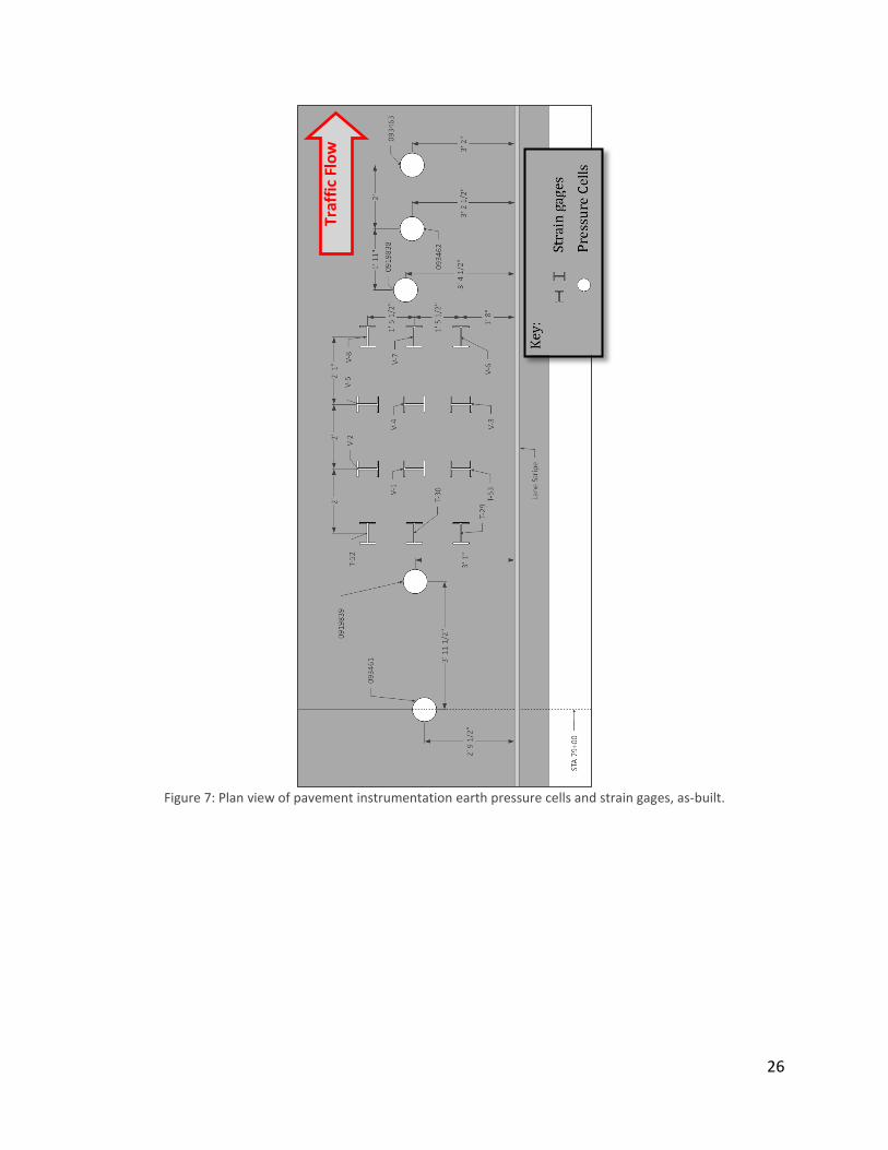
26

Figure 7: Plan view of pavement instrumentation earth pressure cells and strain gages, as-built.

Traf

fic

Flo

w

27

Figure 8: Section view showing locations of pavement instruments within pavement structure.

28

Weather Station Instrumentation

The MEPDG uses detailed historical climatic data for predicting pavement distresses. This data is used to predict temperature and moisture in the layers of the pavement section and also contributes to the smoothness or IRI prediction model. In New Hampshire, there are seven default weather stations to choose from for the MEPDG to generate its climactic file (Applied Research Associates, Inc. 2007). It was determined that it would be beneficial to have a weather station located in close proximity to the instrumented pavement section to supplement existing weather data over the life of the project. The developers of the MEPDG recommend using multiple stations to be sure any gaps in data will be filled by nearby stations (AASHTO 2008). The MEPDG requires hourly averages of temperature, precipitation, wind speed, relative humidity, and cloud cover (AASHTO 2008). In selecting the weather station sensors and accessories, ability to measure those properties were the main concern. Other factors under consideration included, availability, durability, cost and user friendliness. The research team concluded that a modular weather station, provided by Campbell Scientific, would be used. The modular station contains an ambient air temperature sensor, wind speed and direction sensors, a precipitation sensor (rain gage), a solar radiation sensor, a data acquisition system, power system, and a cellular modem. Also included is a stainless steel tripod with a horizontal stainless steel cross-arm for mounting all the sensors. At this time, no relative humidity sensor is present (Steele 2010).

29

Ambient Air Temperature Sensor

The ambient air temperature sensor is a Campbell Scientific Model 107 Temperature Probe with an RM Young 6-Plate Gill Solar Radiation Shield (Figure 9). The radiation grill is used to allow air to pass through to the sensor but shade it from solar radiation thus keeping it as close to the ambient air temperature as possible. The Model 107 is a general purpose temperature probe that consists of a BetaTherm 100K6A thermistor encapsulated in an aluminum housing.The resistance of the thermistor varies with changes in temperature, which, using the Stienhart-Hart equation, can be used to calculate the temperature from the resistance recorded by the data acquisition system (Steele 2010). The Model 107 has an operational measurement range of -35° to 50°C (-31°F to 122°F).

Figure 9: Model 107 temperature probe and radiation grill.

Solar Radiation Sensor

The solar radiation sensor is an Apogee Instruments CS 300 Pyranometer which measures incoming solar radiation with a photovoltaic detector (Figure 10). The instruments measurement range has a maximum of 2000 W/m2, with full sunlight measuring approximately 1000 W/m2 (Steele 2010).

Figure 10: CS 300 pyranometer and lead cables.

Precipitation Sensor

The TE525 Tipping Bucket Rain Gage is an adaptation of the standard Weather Bureau tipping bucket rain gage with a 6 inch collector and an accuracy of 0.01 inches (Burton Jr. and Pitt 2002). Precipitation amounts are determined by a small bucket beneath the collector that tips each time it is filled with 0.01” of rain. The data acquisition system then counts the number of times that the bucket has tipped and multiplies that by 0.01” to determine the magnitude of the precipitation event (Steele 2010).

30

Figure 11: TE525 gage as installed.

Wind Velocity and Direction Sensor

The 03002 R.M. Young Wind Sentry Set (Figure 12) was selected to monitor wind velocity and direction. This set consists of a 03101 R.M. Young Wind Sentry Anemometer and an 03301 R.M. Young Wind Sentry Vane. The anemometer produces a voltage proportional to the wind speed which is then recorded by the data acquisition system. The vane position is determined using a 10kΩ potentiometer with a precision excitation voltage applied (Steele 2010).

Figure 12: Wind Sentry Set as installed.

Power Supply

The weather station makes use of a Campbell Scientific CR1000 data logger powered by a Campbell Scientific PS100 12-volt, 7 amp-hour battery (with charging regulator) and a Campbell Scientific SP20 20-watt Solar Panel. The power system has been designed so that the battery can be continuously float-charged, preventing it from dropping below 10.5 volts (Steele 2010).

31

Figure 13: CR1000 and PS100 power supply inside cabinet.

Figure 14: SP20 solar panel installed on weather station.

Data Acquisition, Storage and Communications

Remote access is achieved with a Raven XTV CDMA Sierra Wireless cellular modem with service provided by Verizon Wireless. The CR1000 is equipped with 4MB of SRAM. The weather station data are stored on the data acquisition system then transmitted via cellular modem to the data computer at UNH. The cellular modem is programmed to only turn on at certain times during the day to save power. Data can be downloaded at any time while the modem is operational (Steele 2010).

Weather Station Configuration

The weather station sensor configuration allows for each sensor to collect data with a minimum amount of interference from the other sensors, the sensor cross-arm, or the tripod mount itself. The sensors were placed on the tripod and the tripod was located with guidance from each sensors’ manufacturer provided installation recommendations along with general guidance from Campbell Scientific (Campbell Scientific, Inc. 1997). The solar radiation sensor was placed on the southern end of the sensor cross-arm with its cable oriented north/south. It was mounted level on a leveling plate that includes a bubble level to ensure accurate measurements. The next sensor to the north on the

32

cross-arm is the air temperature sensor with the radiation grill. The sensor was inserted into the radiation grill taking care that the measurement portion of the sensor was not in contact with the grill and the unit was mounted on the cross-arm. The precipitation gage was mounted at the center of the cross-arm, just to the south of the tripod mast. It is mounted without obstruction above except for the lightning ground rod. The wind speed and direction sensors were placed on the Northern end of the sensor cross-arm with the direction vane at the northern-most end (Steele 2010). Prior to field installation, the tripod was assembled with the sensor cross arm in the laboratory at UNH. At this time all the sensors were mounted and tested for proper functionality outside the lab. They were all connected to the data logger and weather data was collected for a short period of time. It was determined that all the sensors were functioning within the proper ranges and that the factory calibrations would be used for these sensors without offsets. Due to the nature of the Campbell Scientific data logging program, alteration of the calibrations is not trivial, however, if discrepancies were discovered, offsets to the acquired data could be applied (Steele 2010).

Weather Station Siting

The weather station site was chosen by generally applying the guidelines set forth by the manufacturer (Campbell Scientific, Inc. 1997). In addition to those guidelines, the research team chose a level location that could be accessed with relative ease all year while remaining in close proximity to the in-road sensors. Concerns of vandalism were also considered and as a result the instrument cabinet is securely locked and the station is located in an exposed location for visual monitoring. The site chosen is located south of the in-road sensors, in the vicinity of Station 66+00. It is located on the west side of Route 16 on a level area, elevated above the roadway, within the roadway easement (Steele 2010). The weather station sensors were installed on a 10ft tall stainless steel tripod. The tripod base has a 7 ft diameter with the legs extended. With guy wires installed, it has a wind gust tolerance of 100 mph and can resist sustained winds of 80 mph. The tripod was placed in an unobstructed location where it was secured using 12” long spikes driven into the ground. The tripod mast was carefully plumbed and the sensor cross arm was installed. The arm was leveled to ensure proper operation of all sensors (Steele 2010). In the field, the sensor cross arm was installed precisely in north south orientation with the wind speed and direction sensors placed at the northern end. Approximately halfway down the tripod mast the solar cell was installed following the manufacturer recommendations for tilt and orientation. It was then wired to the voltage regulator and power pack contained within the data logger enclosure. The enclosure was mounted on the north side of the tripod, approximately 3 feet above the ground. It contains the power pack and regulator mentioned previously along with the data logger and cellular modem. The antenna for the cellular modem is mounted on the tripod per

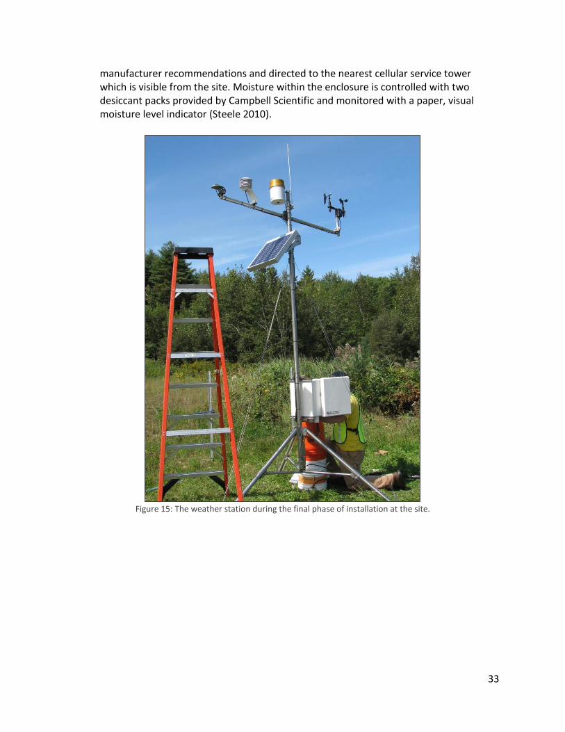
33

manufacturer recommendations and directed to the nearest cellular service tower which is visible from the site. Moisture within the enclosure is controlled with two desiccant packs provided by Campbell Scientific and monitored with a paper, visual moisture level indicator (Steele 2010).

Figure 15: The weather station during the final phase of installation at the site.

Pavement Instrumentation

There were 32 sensors installed in the road at various locations throughout the section. The layout was determined such that the array obtained data from the outside wheel path of the southbound lane. The sensors were also oriented so that longitudinal and transverse strain measurements at the bottom of the asphalt layer could be determined on both sides and in front of and behind the load as it passes over (Steele 2010). The sensor selections were primarily based on cost, sampling rate capacity, and reliability. The sensors also needed to be compatible with the data acquisition systems. Additionally, the sensors were selected based on what has been implemented and maintained at the NCAT Test Track in Auburn, Alabama (Timm, Priest and McEwan 2004, Timm 2009). This allows for an opportunity for collaboration on data collection and troubleshooting if necessary.

Asphalt Temperature Sensors

Three Campbell Scientific Model 108 temperature probes with BetaTherm 100K6A thermistors are used to collect pavement temperature data. These probes have a measurement range of 23°F to 203°F (-5°C to 95° C). The functionality of the Model 108 is identical to the Model 107 probes discussed earlier (Steele 2010).

Figure 16: Campbell Scientific Model 108 probe.

Soil Moisture Sensors

Four Campbell Scientific Watermark 200 soil moisture sensors were installed within the unbound layers. The sensors use an AC half bridge to produce a resistance which is then used to calculate soil water potential within a range of 0 to 200 kPa (Steele 2010).

Figure 17: Campbell Scientific Watermark 200 sensor.

35

Asphalt Strain Sensors

Twelve CTL Group ASG 152 asphalt strain gages were installed in an array at the bottom of the HMA layers. The sensors use a full bridge configuration to which the data acquisition applies an excitation voltage. The voltage signal is recorded. The signal corresponds to a strain measurement. The sensors have an operating temperature range of -29.2°F to 400°F (-34°C to 204°C) and a fatigue life of approximately 105 repetitions at 1500με (Steele 2010).

Figure 18: CTL model ASG 152 strain gage.

Earth Pressure Sensors

Five Geokon Model 3500 earth pressure cells were installed throughout the pavement section. Cells with two pressure ranges (14.5 psi and 36.3 psi), and two pressure plate configurations were used. The cells are constructed with two stainless steel plates, separated by a layer of hydraulic fluid. One pair of pressure cells were constructed with thicker plates for increased durability for use in coarse material. A pressure transducer connected to each cell turns the internal fluid pressure into an electrical signal from 0-100 mV that can be read by the data acquisition system. A calibration is entered which converts the electrical signal to pressure. Each earth pressure cell also contains a thermistor which allows for temperature measurements at each pressure cell location. These thermistors work identically to the Models 107 and 108 temperature probes described previously (Steele 2010).

36

Figure 19: Geokon Model 3500 pressure cell.

Axle Sensors

Two International Road Dynamics Model AS400 axle sensing strips and one AS405 strip were obtained to measure wheel speeds and wheel lateral location. The axle sensing strip produces a change in resistance when a load passes over, the exact timing of which can be determined using the appropriate Dynax SMART interface card and the data acquisition system. The data acquisition system, coupled with the appropriate interface card, can record the time of the resistance change from which speed and lateral location will be calculated (Steele 2010).

Data Acquisition, Storage, and Communication

The in-road sensors make use of two collection systems in order to meet the necessary sampling rate requirements. The strain gages and pressure cells provide “on-demand” real-time data through the use of a DATAQ DI-785 portable chassis. The DI-785 is capable of a total sampling rate of 180kHz, allowing for a maximum per-sensor rate of 9kHz. Previous research suggests that a sampling rate of 5kHz is adequate for the types of sensors used (Timm, Priest and McEwan 2004). Signals from each sensor are processed with DATAQ DI-5B conditioners. The DATAQ DI-785 requires an 110v 60Hz power source, which is provided in the field by a vehicle and an appropriate inverter. The second collection system, for pavement temperature and moisture data, utilizes a Campbell Scientific CR1000 identical to that which is used by the weather station. Both of the in-road acquisition systems are accessed in the field through a physical connection to a Panasonic CF-52 Toughbook laptop (Steele 2010).

37

Figure 20: DATAQ DI-785 with signal conditioners installed.

Figure 21: Campbell Scientific CR1000 in cabinet.

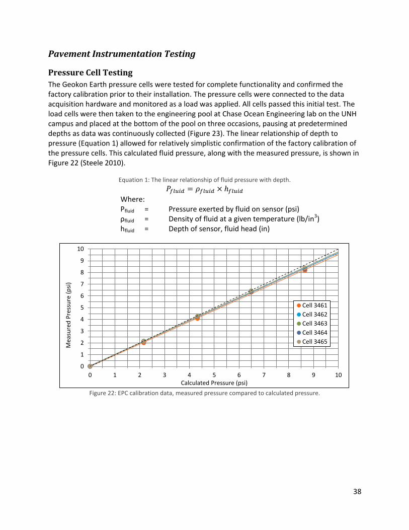
38

Pavement Instrumentation Testing

Pressure Cell Testing

The Geokon Earth pressure cells were tested for complete functionality and confirmed the factory calibration prior to their installation. The pressure cells were connected to the data acquisition hardware and monitored as a load was applied. All cells passed this initial test. The load cells were then taken to the engineering pool at Chase Ocean Engineering lab on the UNH campus and placed at the bottom of the pool on three occasions, pausing at predetermined depths as data was continuously collected (Figure 23). The linear relationship of depth to pressure (Equation 1) allowed for relatively simplistic confirmation of the factory calibration of the pressure cells. This calculated fluid pressure, along with the measured pressure, is shown in Figure 22 (Steele 2010).

Equation 1: The linear relationship of fluid pressure with depth.

Where: Pfluid = Pressure exerted by fluid on sensor (psi) ρfluid = Density of fluid at a given temperature (lb/in3) hfluid = Depth of sensor, fluid head (in)

Figure 22: EPC calibration data, measured pressure compared to calculated pressure.

0

1

2

3

4

5

6

7

8

9

10

0 1 2 3 4 5 6 7 8 9 10

Mea

sure

d P

ress

ure

(p

si)

Calculated Pressure (psi)

Cell 3461

Cell 3462

Cell 3463

Cell 3464

Cell 3465

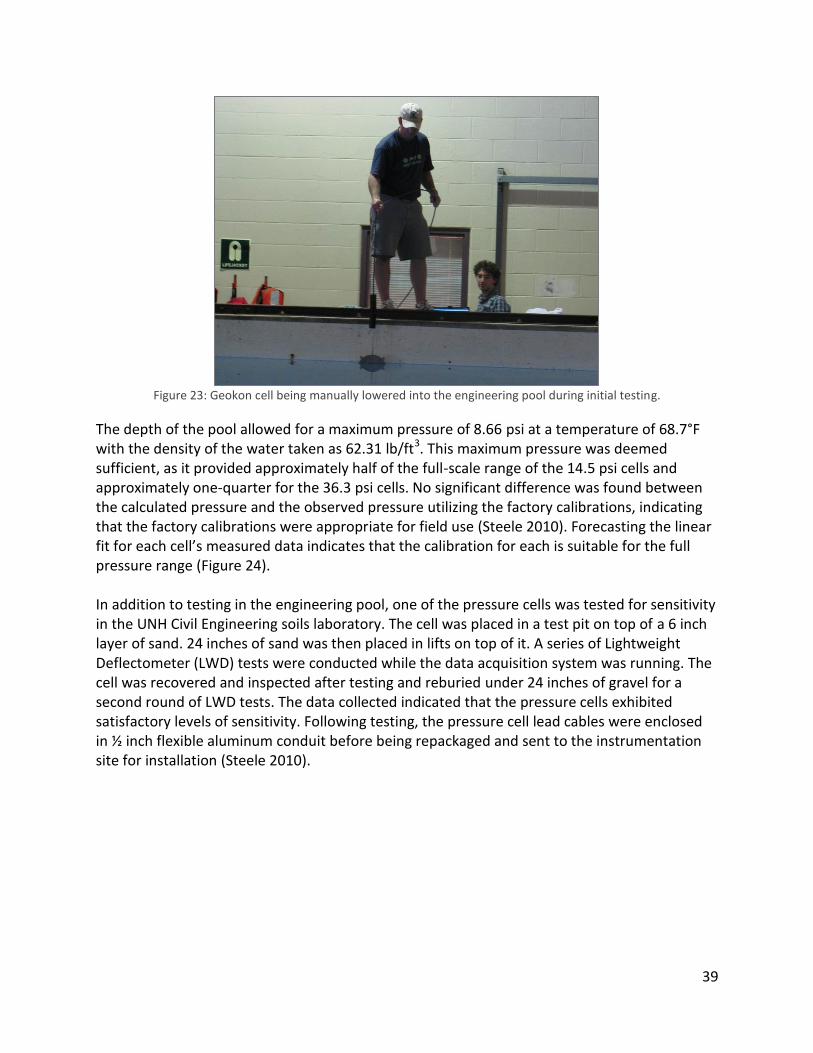
39

Figure 23: Geokon cell being manually lowered into the engineering pool during initial testing.

The depth of the pool allowed for a maximum pressure of 8.66 psi at a temperature of 68.7°F with the density of the water taken as 62.31 lb/ft3. This maximum pressure was deemed sufficient, as it provided approximately half of the full-scale range of the 14.5 psi cells and approximately one-quarter for the 36.3 psi cells. No significant difference was found between the calculated pressure and the observed pressure utilizing the factory calibrations, indicating that the factory calibrations were appropriate for field use (Steele 2010). Forecasting the linear fit for each cell’s measured data indicates that the calibration for each is suitable for the full pressure range (Figure 24).

In addition to testing in the engineering pool, one of the pressure cells was tested for sensitivity in the UNH Civil Engineering soils laboratory. The cell was placed in a test pit on top of a 6 inch layer of sand. 24 inches of sand was then placed in lifts on top of it. A series of Lightweight Deflectometer (LWD) tests were conducted while the data acquisition system was running. The cell was recovered and inspected after testing and reburied under 24 inches of gravel for a second round of LWD tests. The data collected indicated that the pressure cells exhibited satisfactory levels of sensitivity. Following testing, the pressure cell lead cables were enclosed in ½ inch flexible aluminum conduit before being repackaged and sent to the instrumentation site for installation (Steele 2010).

40

Figure 24: EPC calibration data extrapolated to cover the full pressure range for all sensors.

Figure 25: EPC placed in test pit.

14.5 psi

36.3 psi

0

10

20

30

40

0 10 20 30 40

Mea

sure

d P

ress

ure

(p

si)

Calculated Pressure (psi)

Cell 3461

Cell 3462

Cell 3463

Cell 3464

Cell 3465

41

Figure 26: LWD testing being conducted.

Asphalt Strain Gage Testing

The CTL strain gages were connected to the data acquisition system in a laboratory setting. Each strain gage was tested for excessive noise, polarity, and general function. The sensor lead labels were confirmed and “no load” readings were taken. All of the strain gages exhibited acceptable noise levels and registered applied strains properly. Once the functionality was confirmed, the strain gage leads were enclosed in ½ inch flexible aluminum conduit prior to being repackaged and sent to the instrumentation site for installation (Steele 2010).

Axle Sensor Strip Testing

The three axel sensor strips (two AS400 devices and one AS405 device) were delivered to the University of New Hampshire on February 19, 2009, and stored in the Asphalt Materials laboratory. On October 8, 2011, the strips were unpacked and tested with a multimeter in accordance with IRD functionality testing guidelines as there was no record that they had been tested when first received. All three sensor strips exhibited the necessary resistance drops when loaded and met the functionality requirements in the IRD documentation.

Acquisition System Cabling

Given the location of the instrumentation cabinet and the surrounding terrain, a set of 35 foot cables were built to allow for ease of data collection from a vehicle parked down-slope on the soft shoulder of the roadway. The cables are shielded and equipped with screw-on d-subminiature terminals to ensure a secure connection with the data logger (Figure 27). There is no strain-relief device, so care should be taken to properly support both ends of the cable once connected.

42

Figure 27: Custom extension cabling for data acquisition.

Pavement Instrumentation Installation

A number of the in-road sensors were installed one day before the placement of the base HMA course. The majority of the sensor locations and elevations were recorded using GPS equipment provided by the paving contractor. The remaining sensors were placed during the completion of the binder and wearing courses.

Pressure Cell Installation

Due to the location of the various pressure cells within the pavement structure (Figure 8), the pressure cells were installed at different times during the construction. The deepest pressure sensor (093461) was placed after the completion of the compacted 24 inch sand layer by excavating a limited area and positioning and leveling the sensor at the interface between the sand layer and the subgrade. The cabling was routed through a trench cut perpendicular to the direction of travel. The excavation was back-filled and re-compacted by hand. During the same time period, the pressure cell located at the sand/coarse gravel interface (093463) was placed. This process involved a limited-depth excavation at the top of the 24 inch sand layer, followed by a partial back-fill of hand-compacted sand to protect the pressure cell from the 3/8 inch gravel layer that was placed afterwards. Hand-placement of this material served to protect the sensor from construction traffic and from the later placement and compaction of the 12 inch lift of coarse gravel (Steele 2010).

43

Figure 28: Installation of pressure cell 093461.

Cell 093462, located at the interface of the coarse/fine gravel layer (Figure 8), was placed at the top of the coarse gravel layer over a 2 inch lift of sand. After positioning and leveling, the sensor was covered with an additional 2 inch lift of sand followed by 1 inch of 3/8” gravel. The final two pressure cells (0919839 and 0919838) were installed using a similar procedure day before the placement of the asphalt base course (Steele 2010).

44

Moisture Sensor Installation

Moisture sensors were placed at the same time as the pressure cells. The sensors were positioned within the unbound layers and the cabling was routed beneath the pressure cell cable conduit to protect it from construction traffic and the gravel layers (Steele 2010).

Figure 29: Installation of the moisture sensors.

45

Strain Gage Installation

The day before the placement of the asphalt layers, the full array of twelve asphalt strain gages was installed. The strain gages were arranged according to the layout determined by the research team and their cables were buried in shallow trenches dug by hand. After the cables were placed, the trenches were backfilled and compacted by hand using a tamper. One hour before paving, the strain gages were set into, and covered with, a sand and asphalt mixture, as recommended by the manufacturer. The cabling was routed to a junction box outside of the area experiencing construction traffic (Steele 2010).

Figure 30: Pressure cell and strain gages prior to paving.

Figure 31: Strain gage array during base course placement.

46

Strain Gage Troubleshooting

Currently, the pavement strain gages are not fully functional. Troubleshooting efforts undertaken in the field indicate that the problem may lie with the signal conditioning modules in the DATAQ DI-785 chassis, rather than with the gages, interconnects, or cabinet hardware. The DI-785 contains a number of signal conditioning modules which are specific to the type of instrument connected through the input channels that each module corresponds to. Substituting modules for gage channels that were not functioning with known working modules resulted in intermittent functionality.

Axle Sensor Strip Installation

On November 21, 2011, the three sensor strips were transported to the instrumentation site and installed. The original proposed location for the sensor strips is shown along with the modified installation location in Figure 32. The axle sensor strip array was relocated to a new location upstream from the existing pavement instrumentation in order to avoid confounding in measurements and were repositioned within the lane such that wheel wander could be better accounted for (Timm and Priest 2005, Timm and Priest 2004). Locations for the strips were measured from lane stripe and surveyors stakes using chalk lines and marking paint. A gas-powered saw with adjustable-depth diamond blade was used to make three separate pairs of 1.5”-deep cuts through the wearing course. Trenches were cut using hand tools in the soft shoulder and soil to run cables to a junction box located down-slope from the instrumentation cabinet housing the power and acquisition electronics for the in-road sensors. Once cuts were made, wearing course material was removed with an electric impact hammer and the resulting slots and exposed surfaces were blown out with compressed air and brushed clean to ensure a proper bond between the epoxy and the asphalt pavement. Adhesive tape was applied with a 1.0” offset from the edges of each cut.

47

Figure 32: The proposed and as-built location of the axle sensor strip array at the site.

Traffic Flow

48

Figure 33: An adjustable-depth pavement saw being used to cut through the wearing course.

Installation of the sensor strips was performed according to the specifications in the documentation supplied by IRD. Each of the IRD sensor strips was suspended within a wearing surface cut using metal plates and plastic zip-ties provided with the installation kit. Once the strips were properly positioned, a two-part epoxy was prepared from the supplied kit. The epoxy was a Dural 331 which was blended with a fine, uniform sand, then poured into the trenches, leaving the top of each sensor strip exposed and slightly elevated above the surrounding road surface to ensure proper functionality. Although IRD recommended air and pavement minimum temperatures of “50°F and rising”, construction delays and poor weather had moved the installation into late November. Installation was completed with air temperatures ranging from 28°F to 50°F and pavement surface temperatures of 26°F to 58°F (Figure 34). Installation began in the late morning, and was completed in the late afternoon, after both surface and air temperatures had begun to drop measurably.

49

Figure 34: Relevant Temperatures at Site, Nov 21 2011

The lane was opened to traffic two hours and forty five minutes after the second batch of epoxy had been placed and the entire installation was examined approximately four hours after completion to ensure that the epoxy had cured sufficiently. Over the next few weeks, observations were made one to two times per week to ensure that the strips were still bonded to the pavement and that no damage had occurred.

Figure 35: The completed array of axle-sensor strips approximately two weeks after installation.

Lan

e C

lose

d

Surf

ace

Pre

p

Firs

t Ep

oxy

Bat

ch

Lan

e O

pen

ed

Seco

nd

Ep

oxy

Bat

ch

20 °F

25 °F

30 °F

35 °F

40 °F

45 °F

50 °F

55 °F

60 °F

6:00 9:00 12:00 15:00 18:00

Tem

per

atu

re

Time

Asphalt Surface

Air

50

In June 2012, observers at the site reported that snow plows had exposed and damaged one of the sensor strip lead cables that had been routed through the hard shoulder (Figure 36). The damage to the lead cable rendered the sensor strip inoperable. This sensor strip was one of the two parallel ASD400 strips intended to measure vehicle speed, allowing for determination of wheel-path location in conjunction with the diagonal sensor strip. These parallel sensors were made redundant following the installation of the NHDOT Weigh-In-Motion station approximately 100ft upstream of the array location.

Figure 36: Damaged exposed sensor strip loop wires on the hard shoulder.

51

The resulting instrument connectivity is presented in Figure 37. Note that the axle sensor array lead wires currently terminate at the junction box, rather than the instrumentation cabinet, as the cabinet does not currently contain any hardware requiring the sensor strips.

Figure 37: Completed pavement instrument connection diagram.

INSTRUMENTATION CABINET

SIGNAL MULTIPLEXER

DATA LOGGER

DATAQ DI-785

AXLE SENSOR ARRAY

EARTH PRESSURE CELLS

STRAIN GAGES

TEMPERATURE/MOISTURE SENSORS

JUNCTION BOX

LAPTOP IN FIELDLAPTOP IN FIELD

HIGH-SPEED

RS232

52

MEPDG Input Determination

Traffic Data

The NHDOT Bureau of Traffic provided historical traffic reports for a location between Exit 8 and Exit 9 on Route 16, approximately 7 miles south of the instrumentation site. These reports contained 15-minute incremented spot counts broken down by class distribution according to Maine DOT Scheme F. Three reports, from November 2004, August 2007, and July 2010, were provided. The reports covered traffic from 6AM to 6PM at each location, representing approximately 75% of the daily traffic flow, according to NHDOT Traffic Operations Engineer Robert Bollinger. The additional 25% was calculated based on this data and assumed to be evenly distributed across the remaining 12 hours. These numbers were then converted into an hourly percent distribution for the MEPDG. The vehicle class distribution was determined by matching the NHDOT classes (which are identical to the Maine Department of Transportation Scheme F) to the FHWA class descriptions, then to the MEPDG class inputs.

Table 6: Class pairings for NHDOT spot traffic data.

NHDOT “Scheme F” FHWA/MEPDG Class

Bikes Not included in analysis Cars

2 Axle Long Buses Class 4

2 Axle 6 Tire Class 5 3 Axle Single Class 6 4 Axle Single Class 7

< 5 Axle Combo Class 8 5 Axle Combo Class 9

> 6 Axle Combo Class 10 < 6 Axle Multi Class 11 6 Axle Multi Class 12

> 6 Axle Multi Class 13

Traffic growth factors were based upon discussion in the AASHTO Guide for the Design of Pavement Structures and examination of the trends seen in during the years of record (AASHTO 1993). Reductions to the truck traffic volume were made to better represent the site conditions due to the traffic monitoring site being south of the instrumentation site and the differences in traffic volumes at the exits and the changing lane configuration of that section of Route 16 from 2007 to 2010. The monthly adjustment factors for vehicle classes 4 through 13 were left at their default value of 1.00. In the absence of localized Weigh-In-Motion (WIM) data, axle load distribution factors were left as Level 3 defaults. General traffic inputs, consisting of lateral wheel wander, truck axle configurations, single axle configurations, and wheelbase dimensions were left as default.

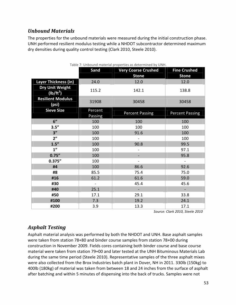
53

Unbound Materials

The properties for the unbound materials were measured during the initial construction phase. UNH performed resilient modulus testing while a NHDOT subcontractor determined maximum dry densities during quality control testing (Clark 2010, Steele 2010).

Table 7: Unbound material properties as determined by UNH.

Sand Very Coarse Crushed Stone

Fine Crushed Stone

Layer Thickness (in) 24.0 12.0 12.0 Dry Unit Weight

(lb/ft3) 115.2 142.1 138.8

Resilient Modulus (psi)

31908 30458 30458

Sieve Size Percent Passing

Percent Passing Percent Passing

6” 100 100 100 3.5” 100 100 100 3” 100 91.6 100 2” 100 - 100

1.5” 100 90.8 99.5 1” 100 - 97.1

0.75” 100 - 95.8 0.375” 100 - -

#4 100 86.6 92.6 #8 85.5 75.4 75.0

#16 61.2 61.6 59.0 #30 - 45.4 45.6 #40 25.1 - - #50 17.1 29.1 33.8

#100 7.3 19.2 24.1 #200 3.9 13.3 17.1

Source: Clark 2010, Steele 2010

Asphalt Testing

Asphalt material analysis was performed by both the NHDOT and UNH. Base asphalt samples were taken from station 78+80 and binder course samples from station 78+00 during construction in November 2009. Fields cores containing both binder course and base course material were taken from station 79+00 and later tested at the UNH Bituminous Materials Lab during the same time period (Steele 2010). Representative samples of the three asphalt mixes were also collected from the Brox Industries batch plant in Dover, NH in 2011. 330lb (150kg) to 400lb (180kg) of material was taken from between 18 and 24 inches from the surface of asphalt after batching and within 5 minutes of dispensing into the back of trucks. Samples were not

54

taken directly from the surface to avoid temperature differentials or segregation of the material. The material was sealed in unlined steel buckets, each containing between 55lb (25kg) and 30kg (65lb) of material, and transported directly to the Materials Laboratory in Kingsbury Hall where the buckets were labeled and stacked until the material was needed for sample fabrication.

Table 8: Summary of HMA properties as measured by NHDOT and UNH.

Asphalt Mix Sample Location AC%

(by weight) AC%

(by volume) Air% Lift Thickness (in)

Surface (12.5mm) Trucks at Plant 5.86 10.84 6.00 1.500 Binder (19.0mm) Sta 78+00 4.66 9.49 4.20 2.250 Base (25.0mm) Sta 79+00, 78+00 4.92 9.79 8.76 2.625

Source: Steele 2010

Sample Preparation

Reheating Procedure

Reheating of the material was performed according to a standardized procedure. The material was heated for one hour in the sealed metal bucket to ten degrees below the discharge temperature specified for each mix (Corti 2011). The lid of the bucket was removed and the material remained in the oven for one additional hour. Following this, the material was divided into pans, each containing roughly 250oz (7100g). These pans were heated to the compaction temperature specified for thirty minutes prior to transfer to the compaction molds.

Table 9: Relevant mix temperatures used during reheating.

Asphalt Mix Discharge Temp (°C) Compaction Temp (°C)

Surface (12.5mm) 160±3 147±2 Binder (19.0mm) 160±3 147±2 Base (25.0mm) 155±3 147±2

Specimen Preparation and Fabrication

Test compactions for the 12.5mm, 19mm, and 25mm mixes were performed to determine the appropriate height/mass ratio to achieve required post-cut/core total voids (air content) of 6% (±0.5%). Therefore, with consideration given to the potential decrease in voids due to coring and cutting, post-compaction specimens were required to have approximately 7% total voids. Specimens then underwent bulk specific gravity testing to develop curves in order to relate compaction height of a known mass to resulting air voids. From these curves, compactions of any mass or height could be prepared to meet the air content requirement. After compaction, air content was verified for each specimen intended for use for dynamic modulus and fatigue testing. Specimens that fell outside of the acceptable range were rejected.

55

The NHDOT Materials and Research lab tested all three mixes and reported bulk specific gravities (Gmb) that differed from those found at UNH using AASHTO T166-05 (Table 10, Figure 38, Figure 39). The reported maximum theoretical specific gravities (Gmm) also differed. The raw specific gravity data has been reproduced in the appendix. To account for these differences, two sets of curves were developed for the test compactions for each mix to ensure proper selection of a height/mass ratio (see Appendices). Specimens were fabricated based on the UNH lab’s findings for maximum theoretical specific gravity (Gmm).

Table 10: Comparison of average Gmm and Gmb values found by the NHDOT and by UNH.

Gmm Gmb

NHDOT UNH NHDOT UNH

12.5mm 2.267 2.401 2.429 2.266

19.0mm 2.457 2.370 2.336 2.325

25.0mm 2.460 2.430 2.345 2.307

Figure 38: Bulk specific gravities of all three mixes as measured by NHDOT and UNH.

2.20

2.25

2.30

2.35

2.40

2.45

2.50

12.0 14.5 17.0 19.5 22.0 24.5

Bu

lk S

pec

ific

Gra

vity

(G

mb

)

Mix NMSA

NHDOT UNH NHDOT Avg UNH Avg

56

Figure 39: Maximum theoretical specific gravity of all three mixes as measured by NHDOT and UNH.

Following compaction, specimens were cored to a diameter of 100mm and cut to a height of 150mm (Figure 40). The bulk specific gravity of each specimen was again evaluated to ensure that the specimen met the 6% (±0.5%) total voids requirement for testing. Six hexagonal steel studs were attached with two-part epoxy in pairs 120° apart using a purpose-built jig (Figure 41) to allow for secure mounting of LVDTs. The epoxy was allowed to cure for a minimum of 36 hours.

Figure 40: Cored, cut, and studded specimen dimensions.

2.20

2.25

2.30

2.35

2.40

2.45

2.50

12.0 14.5 17.0 19.5 22.0 24.5

Max

ium

Sp

ecif

ic G

ravi

ty (

Gm

m)

Mix NMSA

NHDOT UNH NHDOT Avg UNH Avg

57

Figure 41: Cut and cored specimen with LVDT studs being attached.

Dynamic Modulus Testing

Dynamic modulus testing was performed using an IPC Global Asphalt Mixture Performance Tester (AMPT) in order to provide data for the development of master curves and for the Asphalt Material Properties in the MEPDG. Testing was performed across a range of five temperatures and six frequencies for each sample, with a minimum of four specimens (replicates) for each mix design. Samples were initially conditioned at 39°F (4°C) for eighteen to twenty four hours in an environmental chamber. Samples were removed from the chamber and tested with the AMPT before being returned to the chamber and left to reach 70°F (21°C) over a period of approximately three hours. Once tested at this second, higher temperature, they were returned to the chamber and allowed to reach 100°F (37.7°C) before the final round of testing. Following each test, both the specimen and the data were examined for consistency. If inconsistencies were noted, the data was discarded and the specimen was re-tested after a physical examination. On one occasion (Sample B1915) the epoxy bond between an LVDT stud and the specimen failed during 40°F (4.4°C) testing. Post-test examination showed that the stud had been placed at a location where a piece of aggregate was just beneath a thin film of binder, and that there was insufficient bond between the binder at the surface of the stud location and aggregate just under the surface. Additional failures occurred during supplementary rounds of testing at 130°F (54.4°C) (which was not used in the development of the master curves) when

58

the structural integrity of the mix itself began to degrade at locations where the LVDT studs had been attached. In the case of the stud failure on B1915, all of the studs were removed and reattached after rotating the sample approximately 15° to ensure proper attachment locations and the specimen was re-tested. In the cases of the stud failures at the elevated test temperature, the specimens were discarded entirely. The replicates were averaged at each frequency, providing dynamic modulus values for each frequency at each temperature for all of the mixes. Shift factors were determined (see appendices, pages 118-120), using a reference temperature of 70°F (21.1°C) and a sigmoidal fit was established from the shifted data to provide the master curves.

Figure 42: Dynamic modulus master curve for the 12.5mm surface course.

Figure 43: Dynamic modulus master curve for the 19.0mm binder course.

0.0

2.0

4.0

6.0

8.0

10.0

12.0

14.0

1.E-03 1.E-02 1.E-01 1.E+00 1.E+01 1.E+02 1.E+03 1.E+04

Dyn

amic

Mo

du

lus,

|E*

| (G

Pa)

Reduced Frequency (Hz)

4.4 C 21.1 C 37.8 C Sigmoidal Fit

0.0

2.0

4.0

6.0

8.0

10.0

12.0

14.0

1.E-03 1.E-02 1.E-01 1.E+00 1.E+01 1.E+02 1.E+03 1.E+04

Dyn

amic

Mo

du

lus,

|E*

| (G

Pa)

Reduced Frequency (Hz)

4.4 C 21.1 C 37.8 C Sigmoidal Fit

59

Figure 44: Dynamic modulus master curve for the 25.0mm base course.

The MEPDG requires dynamic modulus data points for a temperature between 10°F and 20°F. The IPC AMPT is capable of sustained temperatures as low as 39°F (4°C). In order to test at 20°F (-6.7°C), samples were conditioned in the Espec BTL433 environmental chamber for 12+ hours at 19°F (-7.2°C), then transferred to the IPC chamber at 40°F (4.4°C) and tested immediately to avoid any significant increase in temperature beyond the target of 20°F (-6.7°C). This procedure was confirmed with a dummy asphalt specimen of similar dimensions and an embedded thermocouple. This data was compared to empirical back-calculations for dynamic modulus based upon the testing at the three higher temperatures (4.4°C, 21.1°C, 37.8°C) and found to be satisfactory. Limited testing was undertaken at 130°F (54.4°C), however this data was not used in the analysis due to the weakening of the binder at this elevated temperature.

0.0

2.0

4.0

6.0

8.0

10.0

12.0

14.0

1.E-03 1.E-02 1.E-01 1.E+00 1.E+01 1.E+02 1.E+03 1.E+04

Dyn

amic

Mo

du

lus,

|E*

| (G

Pa)

Reduced Frequency (Hz)

4.4° C 21.1° C 37.8° C Sigmoidal Fit

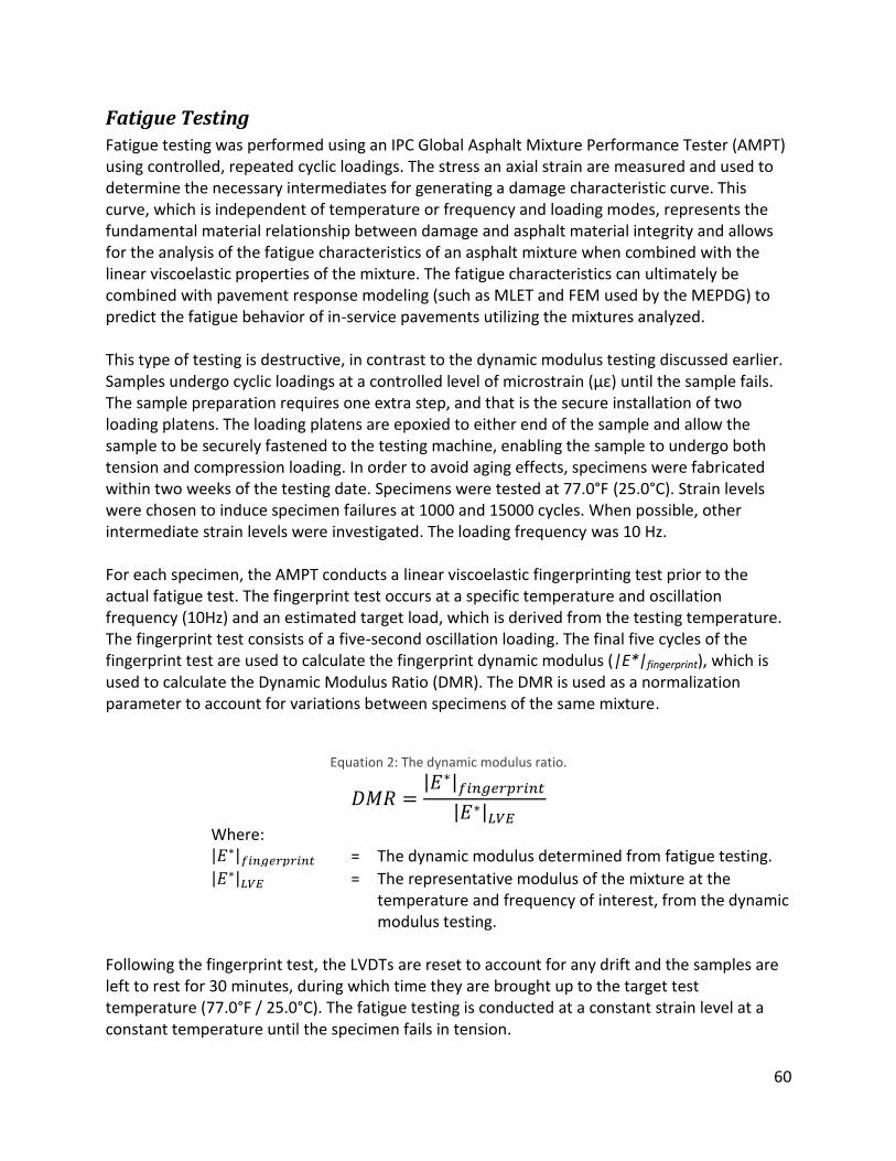
60

Fatigue Testing

Fatigue testing was performed using an IPC Global Asphalt Mixture Performance Tester (AMPT) using controlled, repeated cyclic loadings. The stress an axial strain are measured and used to determine the necessary intermediates for generating a damage characteristic curve. This curve, which is independent of temperature or frequency and loading modes, represents the fundamental material relationship between damage and asphalt material integrity and allows for the analysis of the fatigue characteristics of an asphalt mixture when combined with the linear viscoelastic properties of the mixture. The fatigue characteristics can ultimately be combined with pavement response modeling (such as MLET and FEM used by the MEPDG) to predict the fatigue behavior of in-service pavements utilizing the mixtures analyzed. This type of testing is destructive, in contrast to the dynamic modulus testing discussed earlier. Samples undergo cyclic loadings at a controlled level of microstrain (µε) until the sample fails. The sample preparation requires one extra step, and that is the secure installation of two loading platens. The loading platens are epoxied to either end of the sample and allow the sample to be securely fastened to the testing machine, enabling the sample to undergo both tension and compression loading. In order to avoid aging effects, specimens were fabricated within two weeks of the testing date. Specimens were tested at 77.0°F (25.0°C). Strain levels were chosen to induce specimen failures at 1000 and 15000 cycles. When possible, other intermediate strain levels were investigated. The loading frequency was 10 Hz. For each specimen, the AMPT conducts a linear viscoelastic fingerprinting test prior to the actual fatigue test. The fingerprint test occurs at a specific temperature and oscillation frequency (10Hz) and an estimated target load, which is derived from the testing temperature. The fingerprint test consists of a five-second oscillation loading. The final five cycles of the fingerprint test are used to calculate the fingerprint dynamic modulus (|E*|fingerprint), which is used to calculate the Dynamic Modulus Ratio (DMR). The DMR is used as a normalization parameter to account for variations between specimens of the same mixture.

Equation 2: The dynamic modulus ratio.

| | | |

Where: | | = The dynamic modulus determined from fatigue testing. | | = The representative modulus of the mixture at the

temperature and frequency of interest, from the dynamic modulus testing.

Following the fingerprint test, the LVDTs are reset to account for any drift and the samples are left to rest for 30 minutes, during which time they are brought up to the target test temperature (77.0°F / 25.0°C). The fatigue testing is conducted at a constant strain level at a constant temperature until the specimen fails in tension.

61

The AMPT records a number of parameters every ten cycles (1 second) over the duration of the test. This data includes the dynamic modulus, the phase angle, and a number of load-related parameters. The load-related data includes the minimum, maximum, and average values for the peak-to-peak stress, strain, and applied loads. The data from the AMPT is used as the input for the ALPHA Fatigue software to determine the fatigue characteristics of each specimen and the resulting performance of the mixture. Results from the ALPHA Fatigue analysis are reported in Table 11.

Table 11: IPC AMPT Fatigue testing parameters and results.

NMSA (mm)

Specimen Temperature

(°C) Frequency

(Hz) |E*|LVE (MPa)

|E*|fingerprint (MPa)

DMR Target

µε C at

Failure Failure Cycle

12.5

B1201 25.4 10 2757.4 3320 1.204 650 0.395 815

B1204 25.1 10 2889.2 3724 1.289 400 0.069 15710

B1206 25.1 10 3415.5 3891 1.139 500 0.137 6075

B1209 24.6 10 3349 3439 1.027 600 0.111 3615

19.0

B1910 25.1 10 3295.5 4497 1.365 425 0.135 2455

B1911 24.7 10 3445.3 5440 1.579 375 0.105 3155

B1914 24.1 10 3743.9 4337 1.158 300 0.334 14112

B1916 25.2 10 3158.5 4877 1.544 600 0.395 415

25.0 B2501 25.3 10 3866.9 4076 1.054 275 0.372 18506

B2502 25.1 10 3620.2 3831 1.058 450 0.373 1575

62

Mechanistic-Empirical Pavement Design Guide Analysis

Analysis Explanation

The purpose of this analysis was not to necessarily determine the condition of the pavement section after a set period of time or a predetermined design life, but to evaluate the behavior of the MEPDG and the changes in the predicted performance over an extended analysis period and to investigate the performance of various surface course thicknesses. For this approach, the highest level of analysis was used wherever possible, and the pavement performance was tracked far beyond the normal distress thresholds. This allowed for examination of the stability and suitability of the MEPDG in its current state (as of the time of writing, this was Version 1.100). This extended analysis revealed undocumented model behaviors and program stability issues. The analysis also provided insight into the performance gains attributable to thicker surface courses. This analysis also provided some understanding of what surface course thickness would be required to reduce various distresses, if the existing structure should be considered to be under-designed.

Design Life (Analysis Period)

Typically, the MEPDG analysis uses a parameter called "Design Life", which is defined as "[T]he time from initial construction until the pavement has structurally deteriorated to the point when significant rehabilitation or reconstruction is needed." In the case of this analysis, it is more accurate to refer to this parameter as the "analysis period", as the goal of the analysis is to investigate the behavior of the pavement (within the MEPDG) up to and beyond the pavements intended design life. For this project, the analysis period is 20 years.

Pavement Structure

The pavement structure evaluated consisted of three HMA layers: a variable-thickness surface course, a 2-inch thick binder course, and a 2.625-inch thick base course. Beneath the HMA layers was a 12-inch thick unbound layer of crushed stone followed by a 12-inch layer of coarse crushed stone and a semi-infinite (for the purposes of the analysis) layer of sand.

Construction Delays and Traffic Open Date

Although the MEPDG can simulate the effects of unbound aggregate layer exposure in cases where a delay between unbound layer construction and asphalt placement occurs, the MEPDG cannot evaluate staged construction conditions where intermediate asphalt layers are exposed to traffic loadings before the completion of the pavement structure (AASHTO 2008). This is worth considering for this particular project, as intentional deferment of the wearing course placement lead to the exposure of the intermediate structure to traffic loadings. AASHTO recommends using the date of the completion of the surface course as traffic open date in MEPDG. For the analyses performed for this project, the following dates were used:

Base/Subgrade Construction Date: October 2009

Pavement Construction Date: November 2009

Traffic Open Month: October 2011

63

Configuration of Virtual Machines

The MEPDG tends to exhibit instability at various points during the analysis, in both version 1.0 and 1.1. To address this and avoid the lengthy process of reinstallation on Windows 7 systems that store data outside of the programs’ installation directory, two “guest” virtual machines (VMs) were configured using Oracle VirtualBox. The VMs each ran from within the “host” Windows 7 and each was a separate installation of Windows XP SP3. The VMs allowed for the state of the machine to be “frozen” and later restored. One VM was dedicated to running the MEPDG v1.0 and the second to the MEPDG v1.1. This meant that if the MEPDG were to crash during an analysis, the VM could be restored to a previously working state within seconds. This also allowed for parallel analysis – running v1.0 and v1.1 at the same time. To further simplify batching, each VM had access to a directory on the host which was mounted as a virtual drive. The MEPDG files for each analysis run were stored in this directory. Although the MEPDG v1.0 was not capable of working with v1.1 files (lack of forward-compatibility), exports of certain inputs (such as the asphalt layers) could be stored in the shared folder and accessed from within either guest operating system. Following configuration of the two MEPDG guest environments, analysis runs were performed for surface course thicknesses ranging from 1.0 inches to 5.0 inches (with the exception of 3.50 inches), with both Level 1 and Level 3 inputs. The results of these runs were compared to determine relationships between varying input levels, varying surface thicknesses, and between software versions.

APADS Component Error

The initial batch of runs consisted of Level 1 analyses at varying surface course thicknesses in the MEPDG v1.0 and the MEPDG v1.1. The surface course thickness varied from 1.0 inches (the MEPDG minimum AC layer thickness) to 5.0 inches. At 3.5 inches, both versions of the MEPDG were unstable and the Asphalt Pavement Analysis and Design System (APADS) component application would crash during the AC analysis phase, resulting in malformed input field data which would sometimes require the re-installation of the MEPDG in order to perform further runs. In order to approximate the output that would be generated for a 3.50 inch surface course, several alternate surface course thickness inputs were tested and the results for a 3.50 inch thickness were taken from an interpolation of those alternate inputs. APADS was stable for the analysis of 3.45, 3.49, 3.51 and 3.54 inch surface courses for both Level 1 (Table 11) and Level 3 (Table 14). The interpolation results for the Level 1 analysis resulted in the best-fit equations given in Table 13. The results for Level 3 are presented in Figure 46 and Table 15.

64

Table 12: Inputs and Level 1 results used for interpolation

Surface Thickness (in) Performance Criteria Target Predicted

Distress Reliability Distress Reliability

3.45

Terminal IRI (in/mi) 172 80.000 122.80 93.010

Longitudinal Cracking (ft/mi) 2000 80.000 157.00 85.830

Alligator Cracking (%) 25 80.000 0.20 99.999

AC Layers Deformation (in) 0.25 80.000 0.22 64.100

Total Pavement Deformation (in) 0.75 80.000 0.42 99.990

3.49

Terminal IRI (in/mi) 172 80.000 122.90 92.970

Longitudinal Cracking (ft/mi) 2000 80.000 151.00 86.100

Alligator Cracking (%) 25 80.000 0.20 99.999

AC Layers Deformation (in) 0.25 80.000 0.22 63.700

Total Pavement Deformation (in) 0.75 80.000 0.42 99.990

3.51

Terminal IRI (in/mi) 172 80.000 122.80 93.010

Longitudinal Cracking (ft/mi) 2000 80.000 147.00 86.270

Alligator Cracking (%) 25 80.000 0.20 99.999

AC Layers Deformation (in) 0.25 80.000 0.22 64.540

Total Pavement Deformation (in) 0.75 80.000 0.42 99.990

3.54

Terminal IRI (in/mi) 172 80.000 122.70 93.030

Longitudinal Cracking (ft/mi) 2000 80.000 142.00 86.480

Alligator Cracking (%) 25 80.000 0.20 99.999

AC Layers Deformation (in) 0.25 80.000 0.22 64.320

Total Pavement Deformation (in) 0.75 80.000 0.42 99.990

Figure 45: Results of alternative inputs used for interpolation, best-fit equations from Table 13.

0.00

0.10

0.20

0.30

0.40

0.50

100

120

140

160

180

200

3.44 3.45 3.46 3.47 3.48 3.49 3.50 3.51 3.52 3.53 3.54 3.55 Pav

emen

t D

efo

rmat

ion

an

d A

lliga

tor

Cra

ckin

g

IRI a

nd

Lo

ngi

tud

inal

Cra

ckin

g

Surface Course Thickness (in) Terminal IRI (in/mi) Longitudinal Cracking (ft/mi)Alligator Cracking (%) AC Layers Deformation (in)Total Pavement Deformation (in)

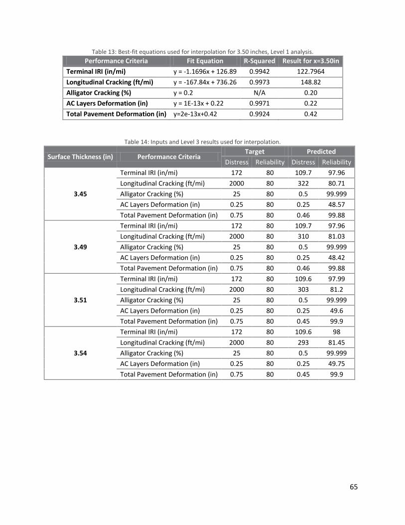
65

Table 13: Best-fit equations used for interpolation for 3.50 inches, Level 1 analysis.

Performance Criteria Fit Equation R-Squared Result for x=3.50in

Terminal IRI (in/mi) y = -1.1696x + 126.89 0.9942 122.7964

Longitudinal Cracking (ft/mi) y = -167.84x + 736.26 0.9973 148.82

Alligator Cracking (%) y = 0.2 N/A 0.20

AC Layers Deformation (in) y = 1E-13x + 0.22 0.9971 0.22

Total Pavement Deformation (in) y=2e-13x+0.42 0.9924 0.42

Table 14: Inputs and Level 3 results used for interpolation.

Surface Thickness (in) Performance Criteria Target Predicted

Distress Reliability Distress Reliability

3.45

Terminal IRI (in/mi) 172 80 109.7 97.96

Longitudinal Cracking (ft/mi) 2000 80 322 80.71

Alligator Cracking (%) 25 80 0.5 99.999

AC Layers Deformation (in) 0.25 80 0.25 48.57

Total Pavement Deformation (in) 0.75 80 0.46 99.88

3.49

Terminal IRI (in/mi) 172 80 109.7 97.96

Longitudinal Cracking (ft/mi) 2000 80 310 81.03

Alligator Cracking (%) 25 80 0.5 99.999

AC Layers Deformation (in) 0.25 80 0.25 48.42

Total Pavement Deformation (in) 0.75 80 0.46 99.88

3.51

Terminal IRI (in/mi) 172 80 109.6 97.99

Longitudinal Cracking (ft/mi) 2000 80 303 81.2

Alligator Cracking (%) 25 80 0.5 99.999

AC Layers Deformation (in) 0.25 80 0.25 49.6

Total Pavement Deformation (in) 0.75 80 0.45 99.9

3.54

Terminal IRI (in/mi) 172 80 109.6 98

Longitudinal Cracking (ft/mi) 2000 80 293 81.45

Alligator Cracking (%) 25 80 0.5 99.999

AC Layers Deformation (in) 0.25 80 0.25 49.75

Total Pavement Deformation (in) 0.75 80 0.45 99.9

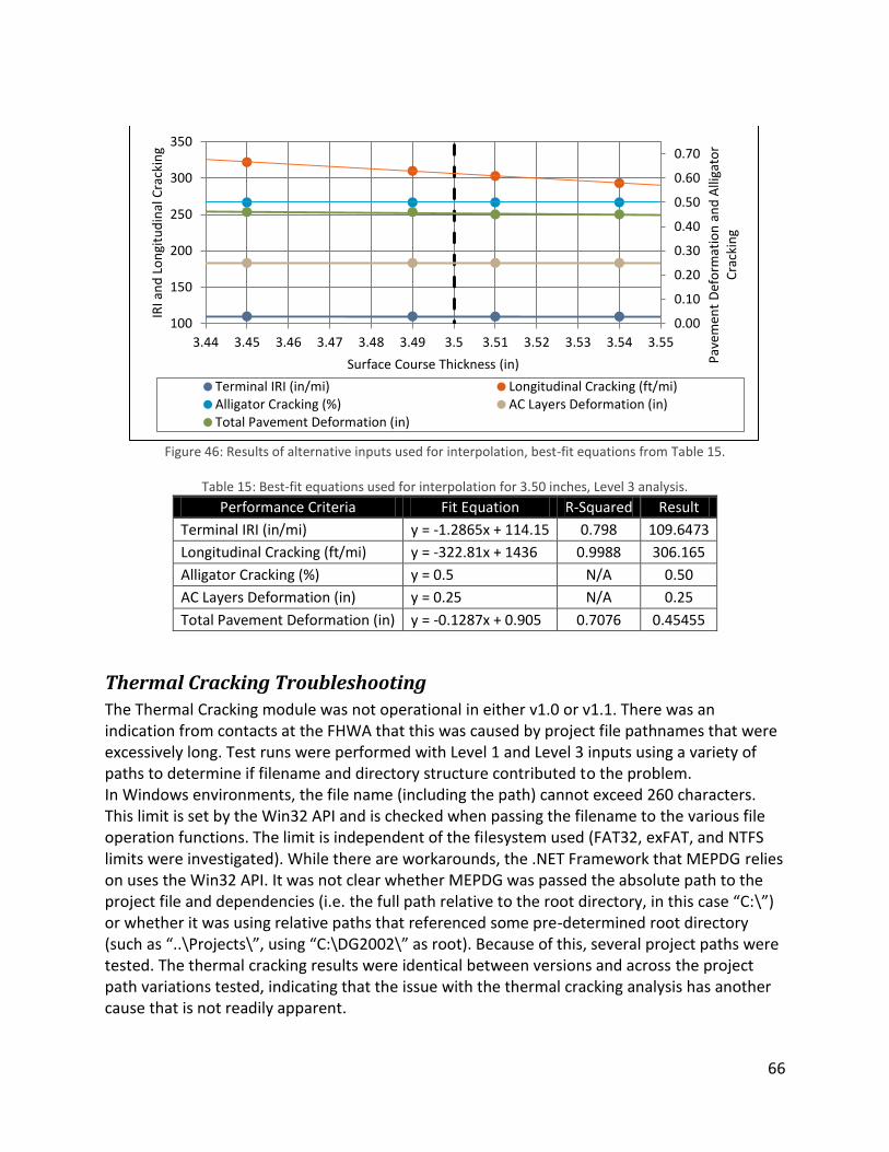
66

Figure 46: Results of alternative inputs used for interpolation, best-fit equations from Table 15.

Table 15: Best-fit equations used for interpolation for 3.50 inches, Level 3 analysis.

Performance Criteria Fit Equation R-Squared Result

Terminal IRI (in/mi) y = -1.2865x + 114.15 0.798 109.6473

Longitudinal Cracking (ft/mi) y = -322.81x + 1436 0.9988 306.165

Alligator Cracking (%) y = 0.5 N/A 0.50

AC Layers Deformation (in) y = 0.25 N/A 0.25

Total Pavement Deformation (in) y = -0.1287x + 0.905 0.7076 0.45455

Thermal Cracking Troubleshooting

The Thermal Cracking module was not operational in either v1.0 or v1.1. There was an indication from contacts at the FHWA that this was caused by project file pathnames that were excessively long. Test runs were performed with Level 1 and Level 3 inputs using a variety of paths to determine if filename and directory structure contributed to the problem. In Windows environments, the file name (including the path) cannot exceed 260 characters. This limit is set by the Win32 API and is checked when passing the filename to the various file operation functions. The limit is independent of the filesystem used (FAT32, exFAT, and NTFS limits were investigated). While there are workarounds, the .NET Framework that MEPDG relies on uses the Win32 API. It was not clear whether MEPDG was passed the absolute path to the project file and dependencies (i.e. the full path relative to the root directory, in this case “C:\”) or whether it was using relative paths that referenced some pre-determined root directory (such as “..\Projects\”, using “C:\DG2002\” as root). Because of this, several project paths were tested. The thermal cracking results were identical between versions and across the project path variations tested, indicating that the issue with the thermal cracking analysis has another cause that is not readily apparent.

0.00

0.10

0.20

0.30

0.40

0.50

0.60

0.70

100

150

200

250

300

350

3.44 3.45 3.46 3.47 3.48 3.49 3.5 3.51 3.52 3.53 3.54 3.55

Pav

emen

t D

efo

rmat

ion

an

d A

lliga

tor

Cra

ckin

g

IRI a

nd

Lo

ngi

tud

inal

Cra

ckin

g

Surface Course Thickness (in)

Terminal IRI (in/mi) Longitudinal Cracking (ft/mi)Alligator Cracking (%) AC Layers Deformation (in)Total Pavement Deformation (in)

67

Results Summary

Reliability summaries for the MEPDG runs have been reproduced below for surface thicknesses in 0.5 inch increments. Full summaries for 0.25 inch increments can be found in the appendices. The outcome column indicates whether the particular pavement structure will exceed a given distress at the specified reliability level (80%). A “fail” indicates that although the predicted level of distress at the end of the analysis period may not necessarily exceed the threshold value, the probability of that distress exceeding it is too great, given the variability within the model. A “pass” basically indicates that for eight out of ten identical projects (80%), the given distress will not reach or exceed the threshold. Table 16 gives the results from the Level 1 20-year analysis, with those distresses that exceed the threshold (at reliability) highlighted in red. Table 17 gives the results from the Level 3 analysis, over the same period. The “Target” columns are the thresholds specified by the NHDOT or given as recommended thresholds by AASHTO, where no agency-specific threshold was recommended. The target 80% reliability level was recommended by the NHDOT. It is important to remember that the predicted distress and predicted reliability columns reflect the terminal pavement conditions at the end of the 20-year analysis period, not at a predetermined end-of-life or the end of the pavement section design life.

68

Table 16: Level 1 reliability summary for the analysis period.

Wearing Course Thickness (in) Performance Criteria Target Predicted

Outcome Distress Reliability Distress Reliability

1.00

Terminal IRI (in/mi) 172 80.000 124.90 91.820 Pass

Longitudinal Cracking (ft/mi) 2000 80.000 872.00 69.880 Fail

Alligator Cracking (%) 25 80.000 1.40 99.999 Pass

AC Layers Deformation (in) 0.25 80.000 0.16 94.240 Pass

Total Pavement Deformation (in) 0.75 80.000 0.41 99.999 Pass

1.50

Terminal IRI (in/mi) 172 80.000 126.40 90.950 Pass

Longitudinal Cracking (ft/mi) 2000 80.000 771.00 71.700 Fail

Alligator Cracking (%) 25 80.000 1.00 99.999 Pass

AC Layers Deformation (in) 0.25 80.000 0.20 74.680 Fail

Total Pavement Deformation (in) 0.75 80.000 0.44 99.970 Pass

2.00

Terminal IRI (in/mi) 172 80.000 123.30 92.760 Pass

Longitudinal Cracking (ft/mi) 2000 80.000 541.00 76.010 Fail

Alligator Cracking (%) 25 80.000 0.70 99.999 Pass

AC Layers Deformation (in) 0.25 80.000 0.19 82.870 Pass

Total Pavement Deformation (in) 0.75 80.000 0.41 99.999 Pass

2.50

Terminal IRI (in/mi) 172 80.000 124.80 91.900 Pass

Longitudinal Cracking (ft/mi) 2000 80.000 394.00 79.050 Fail

Alligator Cracking (%) 25 80.000 0.50 99.999 Pass

AC Layers Deformation (in) 0.25 80.000 0.22 66.620 Fail

Total Pavement Deformation (in) 0.75 80.000 0.43 99.980 Pass

3.00

Terminal IRI (in/mi) 172 80.000 122.30 93.250 Pass

Longitudinal Cracking (ft/mi) 2000 80.000 237.00 83.020 Pass

Alligator Cracking (%) 25 80.000 0.30 99.999 Pass

AC Layers Deformation (in) 0.25 80.000 0.21 70.160 Fail

Total Pavement Deformation (in) 0.75 80.000 0.42 99.990 Pass

3.50*

Terminal IRI (in/mi) 172 80.000 122.80 n/a Pass

Longitudinal Cracking (ft/mi) 2000 80.000 148.82 n/a Pass

Alligator Cracking (%) 25 80.000 0.20 n/a Pass

AC Layers Deformation (in) 0.25 80.000 0.22 n/a Fail

Total Pavement Deformation (in) 0.75 80.000 0.42 n/a Pass

4.00

Terminal IRI (in/mi) 172 80.000 121.00 93.890 Pass

Longitudinal Cracking (ft/mi) 2000 80.000 79.90 90.150 Pass

Alligator Cracking (%) 25 80.000 0.20 99.999 Pass

AC Layers Deformation (in) 0.25 80.000 0.22 67.800 Fail

Total Pavement Deformation (in) 0.75 80.000 0.40 99.999 Pass

4.50

Terminal IRI (in/mi) 172 80.000 121.00 93.920 Pass

Longitudinal Cracking (ft/mi) 2000 80.000 44.00 93.720 Pass

Alligator Cracking (%) 25 80.000 0.10 99.999 Pass

AC Layers Deformation (in) 0.25 80.000 0.22 68.810 Fail

Total Pavement Deformation (in) 0.75 80.000 0.39 99.999 Pass

5.00

Terminal IRI (in/mi) 172 80.000 119.70 94.510 Pass

Longitudinal Cracking (ft/mi) 2000 80.000 21.70 97.240 Pass

Alligator Cracking (%) 25 80.000 0.10 99.999 Pass

AC Layers Deformation (in) 0.25 80.000 0.21 71.950 Fail

Total Pavement Deformation (in) 0.75 80.000 0.38 99.999 Pass

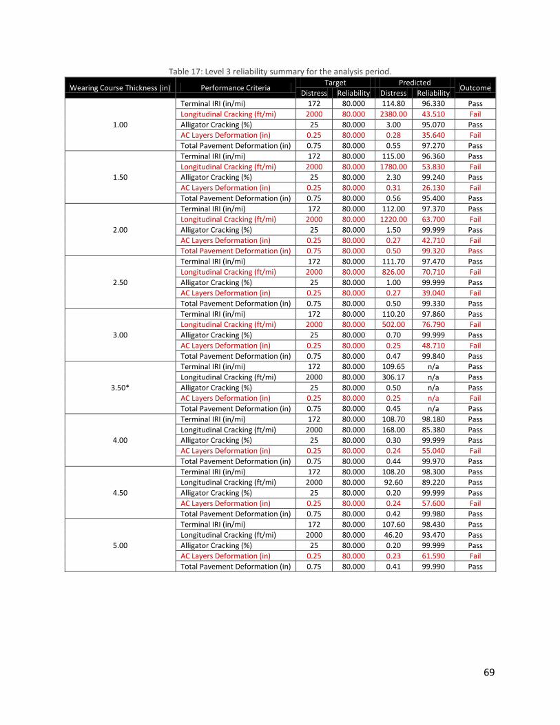
69

Table 17: Level 3 reliability summary for the analysis period.

Wearing Course Thickness (in) Performance Criteria Target Predicted

Outcome Distress Reliability Distress Reliability

1.00

Terminal IRI (in/mi) 172 80.000 114.80 96.330 Pass

Longitudinal Cracking (ft/mi) 2000 80.000 2380.00 43.510 Fail

Alligator Cracking (%) 25 80.000 3.00 95.070 Pass

AC Layers Deformation (in) 0.25 80.000 0.28 35.640 Fail

Total Pavement Deformation (in) 0.75 80.000 0.55 97.270 Pass

1.50

Terminal IRI (in/mi) 172 80.000 115.00 96.360 Pass

Longitudinal Cracking (ft/mi) 2000 80.000 1780.00 53.830 Fail

Alligator Cracking (%) 25 80.000 2.30 99.240 Pass

AC Layers Deformation (in) 0.25 80.000 0.31 26.130 Fail

Total Pavement Deformation (in) 0.75 80.000 0.56 95.400 Pass

2.00

Terminal IRI (in/mi) 172 80.000 112.00 97.370 Pass

Longitudinal Cracking (ft/mi) 2000 80.000 1220.00 63.700 Fail

Alligator Cracking (%) 25 80.000 1.50 99.999 Pass

AC Layers Deformation (in) 0.25 80.000 0.27 42.710 Fail

Total Pavement Deformation (in) 0.75 80.000 0.50 99.320 Pass

2.50

Terminal IRI (in/mi) 172 80.000 111.70 97.470 Pass

Longitudinal Cracking (ft/mi) 2000 80.000 826.00 70.710 Fail

Alligator Cracking (%) 25 80.000 1.00 99.999 Pass

AC Layers Deformation (in) 0.25 80.000 0.27 39.040 Fail

Total Pavement Deformation (in) 0.75 80.000 0.50 99.330 Pass

3.00

Terminal IRI (in/mi) 172 80.000 110.20 97.860 Pass

Longitudinal Cracking (ft/mi) 2000 80.000 502.00 76.790 Fail

Alligator Cracking (%) 25 80.000 0.70 99.999 Pass

AC Layers Deformation (in) 0.25 80.000 0.25 48.710 Fail

Total Pavement Deformation (in) 0.75 80.000 0.47 99.840 Pass

3.50*

Terminal IRI (in/mi) 172 80.000 109.65 n/a Pass

Longitudinal Cracking (ft/mi) 2000 80.000 306.17 n/a Pass

Alligator Cracking (%) 25 80.000 0.50 n/a Pass

AC Layers Deformation (in) 0.25 80.000 0.25 n/a Fail

Total Pavement Deformation (in) 0.75 80.000 0.45 n/a Pass

4.00

Terminal IRI (in/mi) 172 80.000 108.70 98.180 Pass

Longitudinal Cracking (ft/mi) 2000 80.000 168.00 85.380 Pass

Alligator Cracking (%) 25 80.000 0.30 99.999 Pass

AC Layers Deformation (in) 0.25 80.000 0.24 55.040 Fail

Total Pavement Deformation (in) 0.75 80.000 0.44 99.970 Pass

4.50

Terminal IRI (in/mi) 172 80.000 108.20 98.300 Pass

Longitudinal Cracking (ft/mi) 2000 80.000 92.60 89.220 Pass

Alligator Cracking (%) 25 80.000 0.20 99.999 Pass

AC Layers Deformation (in) 0.25 80.000 0.24 57.600 Fail

Total Pavement Deformation (in) 0.75 80.000 0.42 99.980 Pass

5.00

Terminal IRI (in/mi) 172 80.000 107.60 98.430 Pass

Longitudinal Cracking (ft/mi) 2000 80.000 46.20 93.470 Pass

Alligator Cracking (%) 25 80.000 0.20 99.999 Pass

AC Layers Deformation (in) 0.25 80.000 0.23 61.590 Fail

Total Pavement Deformation (in) 0.75 80.000 0.41 99.990 Pass

70

Longitudinal Cracking

Longitudinal cracking is far below the threshold value of 2000 feet/mile for all surface course thicknesses analyzed at Level 1, but surpasses the threshold for the 1.00 through 1.50 in surface courses during the Level 3 analysis (Figure 47). Overall, the Level 3 analysis for longitudinal cracking is far more conservative than the Level 1 analysis (Figure 48). Visible separations between the surface course groupings become apparent when the terminal longitudinal cracking magnitudes are presented. These “gaps” in the distress predictions (such as the separation between 1.75 and 2.00 inches being far greater than the separation between 1.50 and 1.75 inches) are due to the model that the MEPDG uses for longitudinal cracking. These “jumps” in cracking directly influence the terminal IRI prediction behavior described in a subsequent section. The separation is less apparent in the Level 3 analyses, which tend towards a more conservation modeling. The exact reasons for the distress prediction separation are unknown, and would require further research into the modeling functionality of the MEPDG if a better understanding of the behavior was desired.

Figure 47: Longitudinal cracking over the analysis period, Level 1.

0

100

200

300

400

500

600

700

800

900

1000

0 24 48 72 96 120 144 168 192 216 240

Lon

gitu

din

al C

rack

ing

(ft/

mi)

Month of Service

1.00 in1.25 in1.50 in1.75 in2.00 in2.25 in2.50 in2.75 in3.00 in3.25 in3.50 in3.75 in4.00 in4.25 in4.50 in4.75 in5.00 in

71

Figure 48: Longitudinal cracking over the analysis period, Level 3.

Figure 49: Longitudinal Cracking at End-of-Service from both Level 1 and Level 3 inputs.

0

500

1000

1500

2000

2500

0 24 48 72 96 120 144 168 192 216 240

Lon

gitu

din

al C

rack

ing

(ft/

mi)

Month of Service

1.00 in1.25 in1.50 in1.75 in2.00 in2.25 in2.50 in2.75 in3.00 in3.25 in3.50 in3.75 in4.00 in4.25 in4.50 in4.75 in5.00 in

Threshold = 2000 ft/mi

0

500

1000

1500

2000

2500

1.00 1.50 2.00 2.50 3.00 3.50 4.00 4.50 5.00

Lon

gitu

din

al C

rack

ing

(ft/

mi)

Surface Course Thickness (in)

Level 1

Level 3

72

Figure 50: Comparison of Level 1 and Level 3 range of Longitudinal Cracking.

Alligator Cracking

Alligator cracking (as a percentage of total surface area) is several orders of magnitude below the threshold value of 25.0% for all surface course thicknesses analyzed at both levels (Figure 51, Figure 52). Both analyses start to converge on terminal cracking values as the pavement surface course thickness, and therefore total HMA thickness, increases (Figure 54). As expected, the Level 3 analysis produced higher magnitudes of terminal alligator cracking (Figure 53). The overall trend was inversely proportional to the surface course thickness, as thicker pavements tend to experience lower tensile stress and strain at the bottom of the HMA layers (Transportation Research Board 2010).

Figure 51: Alligator cracking over the analysis period, Level 1.

0

500

1000

1500

2000

2500

0 24 48 72 96 120 144 168 192 216 240

Lon

gitu

din

al C

rack

ing

(ft/

mi)

Month of Service

Level 3

Level 1

0.0%

0.2%

0.4%

0.6%

0.8%

1.0%

1.2%

1.4%

0 12 24 36 48 60 72 84 96 108 120 132 144 156 168 180 192 204 216 228 240

Alli

gato

r C

rack

ing

(To

tal L

ane

Are

a)

Month of Service

1.00 in1.25 in1.50 in1.75 in2.00 in2.25 in2.50 in2.75 in3.00 in3.25 in3.50 in3.75 in4.00 in4.25 in4.50 in4.75 in5.00 in

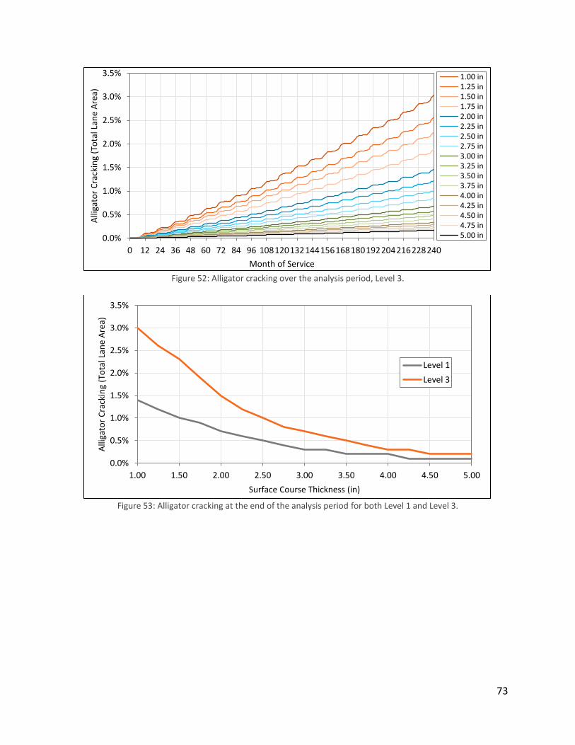
73

Figure 52: Alligator cracking over the analysis period, Level 3.

Figure 53: Alligator cracking at the end of the analysis period for both Level 1 and Level 3.

0.0%

0.5%

1.0%

1.5%

2.0%

2.5%

3.0%

3.5%

0 12 24 36 48 60 72 84 96 108120132144156168180192204216228240

Alli

gato

r C

rack

ing

(To

tal L

ane

Are

a)

Month of Service

1.00 in1.25 in1.50 in1.75 in2.00 in2.25 in2.50 in2.75 in3.00 in3.25 in3.50 in3.75 in4.00 in4.25 in4.50 in4.75 in5.00 in

0.0%

0.5%

1.0%

1.5%

2.0%

2.5%

3.0%

3.5%

1.00 1.50 2.00 2.50 3.00 3.50 4.00 4.50 5.00

Alli

gato

r C

rack

ing

(To

tal L

ane

Are

a)

Surface Course Thickness (in)

Level 1

Level 3

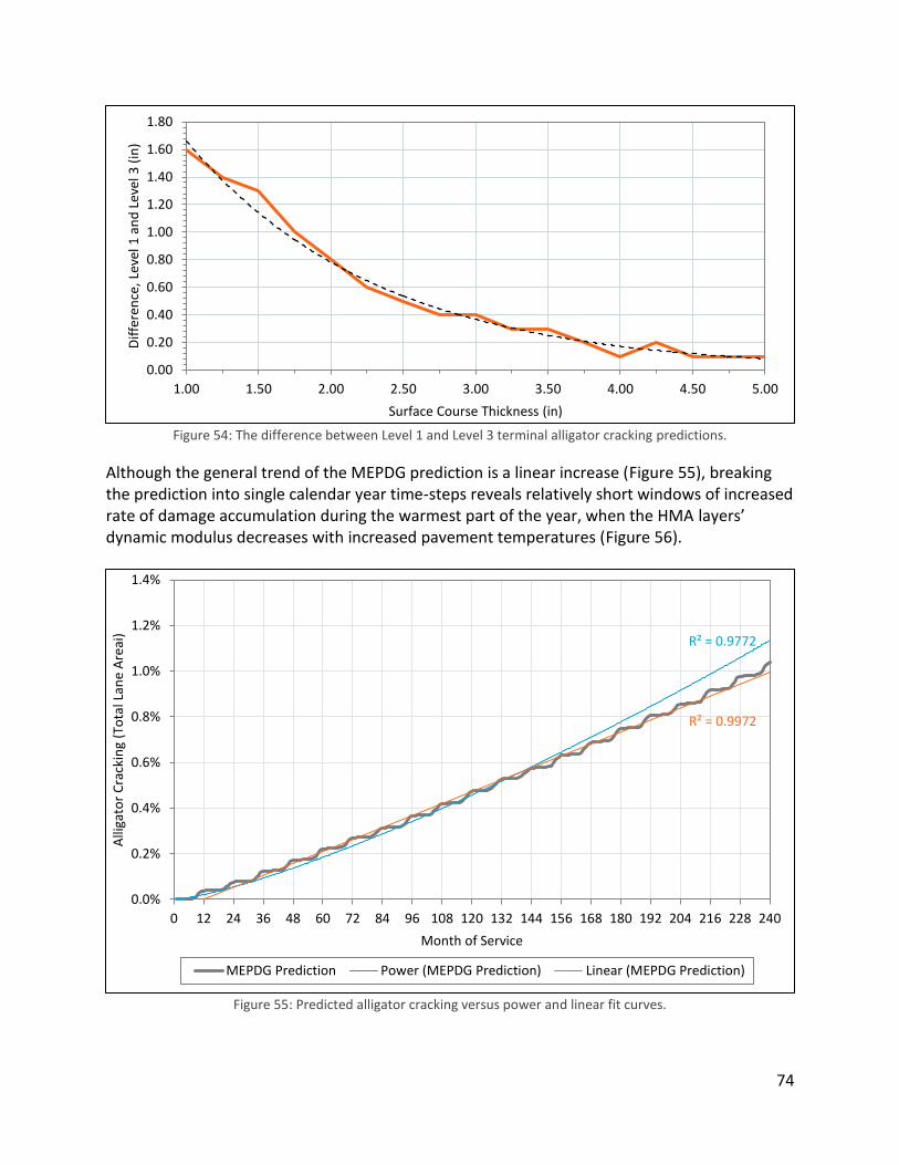
74

Figure 54: The difference between Level 1 and Level 3 terminal alligator cracking predictions.

Although the general trend of the MEPDG prediction is a linear increase (Figure 55), breaking the prediction into single calendar year time-steps reveals relatively short windows of increased rate of damage accumulation during the warmest part of the year, when the HMA layers’ dynamic modulus decreases with increased pavement temperatures (Figure 56).

Figure 55: Predicted alligator cracking versus power and linear fit curves.

0.00

0.20

0.40

0.60

0.80

1.00

1.20

1.40

1.60

1.80

1.00 1.50 2.00 2.50 3.00 3.50 4.00 4.50 5.00

Dif

fere

nce

, Le

vel 1

an

d L

evel

3 (

in)

Surface Course Thickness (in)

R² = 0.9772

R² = 0.9972

0.0%

0.2%

0.4%

0.6%

0.8%

1.0%

1.2%

1.4%

0 12 24 36 48 60 72 84 96 108 120 132 144 156 168 180 192 204 216 228 240

Alli

gato

r C

rack

ing

(To

tal L

ane

Are

ai)

Month of Service

MEPDG Prediction Power (MEPDG Prediction) Linear (MEPDG Prediction)

75

Figure 56: Single calendar year from the MEPDG alligator cracking model.

Research and field observations suggest that this type of distress starts gradually. Then, as the pavement loses structural integrity and the cracks propagate, the rate of distress accumulation increases more rapidly (Huang 2004). The MEPDG distress predictions appear to be closer to a linear trend when viewed over the full analysis period. However, closer inspection of the rate of change (the first derivative of the distress prediction) reveals a linear increase in the rate of change over time once the seasonal fluctuation in the rate of change is accounted for, which is the behavior described by the literature.

Figure 57: Alligator cracking rate of change over the analysis period.

0.00%

0.01%

0.02%

0.03%

0.04%

0.05%

Jan-12 Feb-12 Mar-12 Apr-12 May-12 Jun-12 Jul-12 Aug-12 Sep-12 Oct-12 Nov-12

Alli

gato

r C

rack

ing

(To

tal L

ane

Are

ai)

Month of Service

0

0.005

0.01

0.015

0.02

0.025

0 24 48 72 96 120 144 168 192 216 240

Alli

gato

r C

rack

ing

Rat

e o

f C

han

ge

Month of Service

76

Permanent Deformation

MEPDG calculates total surface deformation due to the plastic (permanent) deformation of the various layers of the pavement structure. The incremental deformation in each layer is estimated for “sub-seasons” at the middle of each layer, as the material properties are greatly affected by temperature and moisture throughout the design life of the pavement (AASHTO 2008). MEPDG also accounts for strain hardening in the material layers as a result of this plastic deformation. This is the modeling step where monthly adjustment factors for traffic volume have the greatest effect on the accumulated deformation in the pavement, as seasonal variation in pavement material properties leads to variable response to repeated loadings. While total permanent deformation remains below the threshold value of 0.75 inches due to the strength of the unbound layers, deformation in the asphalt layers exceeds the threshold value of 0.25 at 80% reliability across a range of surface course thicknesses. The threshold for AC deformation is shown as a function of unbound layer deformation in Level 3 analysis provided conservative estimates of both HMA and unbound layer deformations, as is expected from the MEPDG documentation (AASHTO 2008). At a surface course thickness of 2.75 inches, however, unbound deformation was identical between Level 1 and Level 3 (Figure 60). The MEPDG appears to have greater sensitivity towards the level of analysis with thinner surface course thicknesses, showing greater disparity between the Level 1 and Level 3 predicted deformation in the HMA layers when surface course thicknesses are lower than approximately 2.50 inches for the pavement structure being analyzed.

Figure 58: Permanent Deformation of the pavement structure at end of the analysis period, Level 1.

0.00

0.10

0.20

0.30

0.40

0.50

0.60

1.00 1.25 1.50 1.75 2.00 2.25 2.50 2.75 3.00 3.25 3.50 3.75 4.00 4.25 4.50 4.75 5.00

Per

man

ent

Def

orm

atio

n (

in)

Surface Course Thickness (in)

Total Deformation (Unbound Layers) Total Deformation (HMA Layers) Allowable HMA Deformation

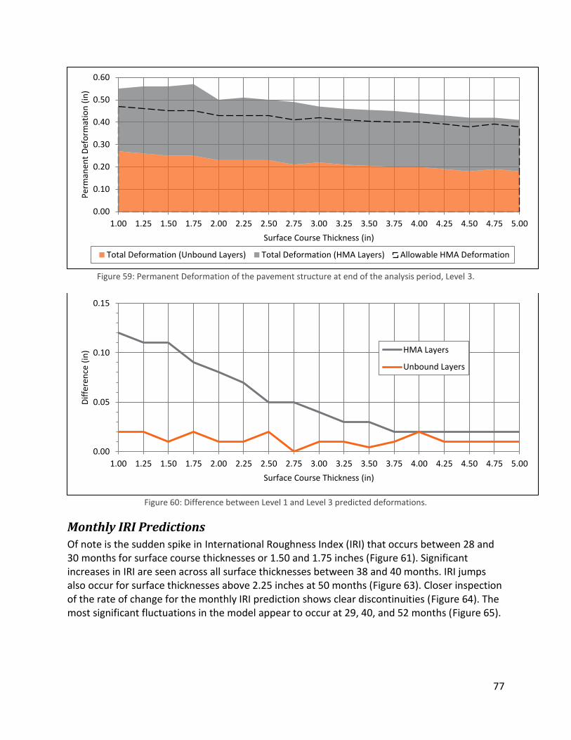
77

Figure 59: Permanent Deformation of the pavement structure at end of the analysis period, Level 3.

Figure 60: Difference between Level 1 and Level 3 predicted deformations.

Monthly IRI Predictions

Of note is the sudden spike in International Roughness Index (IRI) that occurs between 28 and 30 months for surface course thicknesses or 1.50 and 1.75 inches (Figure 61). Significant increases in IRI are seen across all surface thicknesses between 38 and 40 months. IRI jumps also occur for surface thicknesses above 2.25 inches at 50 months (Figure 63). Closer inspection of the rate of change for the monthly IRI prediction shows clear discontinuities (Figure 64). The most significant fluctuations in the model appear to occur at 29, 40, and 52 months (Figure 65).

0.00

0.10

0.20

0.30

0.40

0.50

0.60

1.00 1.25 1.50 1.75 2.00 2.25 2.50 2.75 3.00 3.25 3.50 3.75 4.00 4.25 4.50 4.75 5.00

Per

man

ent

Def

orm

atio

n (

in)

Surface Course Thickness (in)

Total Deformation (Unbound Layers) Total Deformation (HMA Layers) Allowable HMA Deformation

0.00

0.05

0.10

0.15

1.00 1.25 1.50 1.75 2.00 2.25 2.50 2.75 3.00 3.25 3.50 3.75 4.00 4.25 4.50 4.75 5.00

Dif

fere

nce

(in

)

Surface Course Thickness (in)

HMA Layers

Unbound Layers

78

Figure 61: IRI throughout 20-year analysis period across all modeled surface thicknesses, Level 1.

Figure 62: IRI for the first three years (36 months) of pavement life, Level 1.

75

85

95

105

115

125

135

145

155

0 24 48 72 96 120 144 168 192 216 240

Inte

rnat

ion

al R

ou

ghn

ess

Ind

ex (

in/m

i)

Month of Service

1.00 in1.25 in1.50 in1.75 in2.00 in2.25 in2.50 in2.75 in3.00 in3.25 in3.50 in3.75 in4.00 in4.25 in4.50 in4.75 in5.00 in

75

80

85

90

95

100

105

110

0 6 12 18 24 30 36

Inte

rnat

ion

al R

ou

ghn

ess

Ind

ex (

in/m

i)

Month of Service

1.00 in1.25 in1.50 in1.75 in2.00 in2.25 in2.50 in2.75 in3.00 in3.25 in3.50 in3.75 in4.00 in4.25 in4.50 in4.75 in5.00 in

79

Figure 63: IRI for two years to eight years of pavement life, Level 1.

Figure 64: Rate of change of monthly IRI throughout the analysis period, Level 1.

85

90

95

100

105

110

115

120

125

130

24 36 48 60 72 84 96

Inte

rnat

ion

al R

ou

ghn

ess

Ind

ex (

in/m

i)

Month of Service

1.00 in1.25 in1.50 in1.75 in2.00 in2.25 in2.50 in2.75 in3.00 in3.25 in3.50 in3.75 in4.00 in4.25 in4.50 in4.75 in5.00 in

0

2

4

6

8

10

12

14

16

18

0 24 48 72 96 120 144 168 192 216 240

Rat

e o

f C

han

ge, I

nte

rnat

ion

al R

ou

ghn

ess

Ind

ex (

in/m

i/m

on

th)

Month of Service

1.00 in1.25 in1.50 in1.75 in2.00 in2.25 in2.50 in2.75 in3.00 in3.25 in3.50 in3.75 in4.00 in4.25 in4.50 in4.75 in5.00 in

80

Figure 65: Detail of rate of change for month 25 through month 60, Level 1.

Figure 66: IRI throughout 20-year analysis period across all modeled surface thicknesses, Level 3.

In the Level 3 analysis, the 1.00 in surface course appears as an outlier, with monthly IRI predictions lying far outside the range occupied by thicknesses 1.25 in through 5.00 in (Figure 66). The IRI data for that particular analysis was excluded from Figure 67 below to better illustrate the behavior of the MEPDG between the two analysis levels. Level 3 IRI predictions show greater variation between the thinnest and thickest surface courses analyzed, but do not demonstrate the cross-thickness variability illustrated by the abrupt jumps in IRI seen in the Level 1 analysis (Figure 67). The accelerated rate of change seen in month 40 of the design life is readily apparent, seen in Figure 67 as an abrupt jump in predicted IRI range for the Level 1 analysis.

0

2

4

6

8

10

12

14

16

18

25 30 35 40 45 50 55 60

Rat

e o

f C

han

ge, I

nte

rnat

ion

al R

ou

ghn

ess

Ind

ex (

in/m

i/m

on

th)

Month of Service

1.00 in1.25 in1.50 in1.75 in2.00 in2.25 in2.50 in2.75 in3.00 in3.25 in3.50 in3.75 in4.00 in4.25 in4.50 in4.75 in5.00 in

60

70

80

90

100

110

120

130

140

150

0 24 48 72 96 120 144 168 192 216 240

Inte

rnat

ion

al R

ou

ghn

ess

Ind

ex (

in/m

i)

Month of Service

1.00 in1.25 in1.50 in1.75 in2.00 in2.25 in2.50 in2.75 in3.00 in3.25 in3.50 in3.75 in4.00 in4.25 in4.50 in4.75 in5.00 in

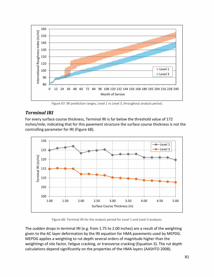
81

Figure 67: IRI prediction ranges, Level 1 vs Level 3, throughout analysis period.

Terminal IRI

For every surface course thickness, Terminal IRI is far below the threshold value of 172 inches/mile, indicating that for this pavement structure the surface course thickness is not the controlling parameter for IRI (Figure 68).

Figure 68: Terminal IRI for the analysis period for Level 1 and Level 3 analyses.

The sudden drops in terminal IRI (e.g. from 1.75 to 2.00 inches) are a result of the weighting given to the AC layer deformation by the IRI equation for HMA pavements used by MEPDG. MEPDG applies a weighting to rut depth several orders of magnitude higher than the weightings of site factor, fatigue cracking, or transverse cracking (Equation 3). The rut depth calculations depend significantly on the properties of the HMA layers (AASHTO 2008).

80

90

100

110

120

130

140

150

160

0 12 24 36 48 60 72 84 96 108 120 132 144 156 168 180 192 204 216 228 240

Inte

rnat

ion

al R

ou

ghn

ess

Ind

ex (

in/m

i)

Month of Service

Level 1

Level 3

100

105

110

115

120

125

130

1.00 1.50 2.00 2.50 3.00 3.50 4.00 4.50 5.00

Term

inal

IRI (

in/m

i)

Surface Course Thickness (in)

Level 1

Level 3

82

Therefore, IRI is a function of four factors: the Site Factor (SF), the total combined area of fatigue cracking (FCtotal), the total length of transverse cracking (TC), and the rut depth (RD).

Equation 3: MEPDG Smoothness for New HMA Pavements.

( ) ( ) ( ) ( )

Where: IRI0 = Initial IRI after construction (in/mi) SF = Site factor FCtotal = Area of combined fatigue cracking as a percentage of total lane area TC = Transverse cracking length (ft/mi) RD = Average rut depth (in)

Although discontinuities are visible in the plots of load-related fatigue cracking, rut depth is weighted the heaviest and has the greatest effect on the IRI. Rut depth is determined by the thickness of the HMA layer or sublayer (hHMA), the number of load repetitions (n), and the pavement temperature (T) during load cycles for each analysis period during the design life (AASHTO 2008). Total accumulated rut depth is the sum of the permanent deformation through all HMA layers/sublayers across all analysis periods:

Equation 4: Accumulated rut depth equation for new HMA pavements

∑ ( ) ∑ ( ) ∑ ( )

Where: Δp(HMA) = Accumulated permanent deformation in the HMA layer/sublayer (in) εp(HMA) = Accumulated permanent axial strain in the HMA layer/sublayer (in/in) εr(HMA) = Elastic strain at the mid-depth of the HMA layer/sublayer (in/in) hHMA = Thickness of the HMA layer/sublayer (in) n = Number of axle-load repetitions T = Pavement temperature (°F) kz = Depth confinement factor k1r,2r,3r Global field calibration parameters from the NCHRP 1-40D recalibration βir,2r,3r = Local field calibration parameters

From Equation 4, there are two parameters that control the rut depth during each analysis period: the thickness of the HMA layer/sublayer (hHMA), which also modifies the strain parameters, and the depth confinement factor (kz). The depth confinement factor is controlled by the total thickness of all HMA layers/sublayers (as a component of parameters C1 and C2) and the depth below the pavement surface of the HMA layer/sublayer (again, affected by the total HMA layer/sublayer thickness).

83

Equation 5: Depth confinement factor for permanent deformation calculation.

( )

Where: C1 = -0.1039(HHMA)2 + 2.4868 HHMA – 17.342 C2 = -0.0172(HHMA)2 + 1.7331 HHMA – 27.428 D = Depth below the surface (in) HHMA = Total thickness of the HMA layers/sublayers (in)

From Equation 3, Equation 4, and Equation 5, IRI for the pavement structure analyzed appears to be largely controlled by the average rut depth, which is turn largely determined by the thickness of all of the HMA layers and the surface layer thickness in particular. Influence of the depth confinement factor (kz) appears to dramatically increase with increasing HMA surface course thickness.

84

Local Calibration

The transfer functions within the MEPDG are the most important components for relating modeled predictions of distresses to field observations in order to improve the accuracy of the MEPDG. Validation of the distress predictions is an important step in establishing confidence in the MEPDG modeling and requires calibration of these transfer functions using independent field observations of modeled pavement sections. Calibration reduces the difference between the model’s distress predictions and the actual distresses and reduces or eliminates bias in the prediction models, resulting in reduced construction costs and better reliability (AASHTO 2008, AASHTO 2010). The MEPDG’s performance models were calibrated using “global” data from the Long Term Pavement Performance (LTPP) database, but AASHTO recommends the development and implementation of calibration procedures to account for variability in local conditions, materials, and construction methods which may differ significantly from those at the LTPP database test sections (AASHTO 2010).The performance models themselves are based on mathematical models and mechanics principles that are assumed to provide a relatively accurate and correct simulation of real-world conditions and material behaviors. AASHTO has developed a comprehensive process for local calibration, which involves everything from initial agency policy decisions, to experimental design and observation, to the assessment of bias and the final calibration of the MEPDG transfer functions (AASHTO 2010). The approach is broken down into eleven steps, outlined in Table 18 below. The calibration approach is provided here as a functional summary, but the AASHTO Guide for the Local Calibration of the MEPDG should be consulted for greater detail.

Table 18: AASHTO Local calibration procedure summary for the MEPDG.

Step Description 1 Selection of Input Levels for Agency Design and Analysis

2 Development of Experimental Matrix

3 Estimation of Sample Sizes for Distress Models

4 Selection of Roadway Segments

5 Extraction and Evaluation of Roadway Segment Test Data

6 Field Investigation of Test Sections

7 Bias Assessment

8 Local Bias Elimination

9 Standard Error Assessment

10 Model Precision Improvement

11 Interpretation of Results and Confirmation of Calibration

Source: AASHTO 2010

85

Step 1: Selection of Input Levels for Agency Design and Analysis

The selection and/or determination of the appropriate input levels is typically an agency policy decision, driven by the field monitoring and laboratory testing capabilities available. The existing material specifications and construction methods also can also influence the decisions made during this step. Varying input levels can be chosen for use, and the decisions made ultimately will influence the final standard error seen in each distress prediction model. Consideration should be given to material specifications and construction costs during this step, as well, because pursuing Level 1 hierarchal inputs may not be cost-effective, if the particular input introduces little error in the final predictions.

Step 2: Development of an Experimental Matrix

The initial phase of local calibration requires the development of a statistically-sound sampling plan in order to properly calibrate and refine the distress prediction models in an efficient and cost-effective manner. The goal of the development of the sampling plan is to determine if the bias or the standard error of the transfer function for each distress is dependent in any way on the design parameters. This sampling plan should be based on local conditions and address three objectives:

1. Determination of the local bias (if any) present in the distress predictions or simulation models.

2. Determination of the cause of the biases. 3. Determination of the appropriate local calibration coefficients or transfer

functions. The parameters in the experimental matrix should be divided into primary and secondary tiers. The primary tier should consist of the factors of greatest interest and greatest effect on performance. Examples of primary tier parameters are: pavement type, surface type, structure thickness, and subgrade soil type. Climate may also be considered a primary parameter if significant environmental variability exists within the region where the calibration is being performed. Secondary parameters generally include those design factors which are typically not independent from primary parameter changes, such as traffic level or pavement-type-specific design features (traffic level often determines structure thickness). AASHTO recommends the use of replicate roadway segments for most of the cells in the experimental matrix to provide a better estimate of the pure error.

Step 3: Estimation of Sample Sizes

Bias and precision are both important to the local calibration procedure, therefore the number of evaluations needed to validate the prediction model needs to be determined for both bias and precision, independently. It is important to note that there is a coupling effect between the different distresses, and as a result, the same test sections should be used for all distresses calibrations if possible. However, the MEPDG assumes

86

that the magnitude and occurrence of each distress is independent of the other distresses (uncoupled), with the exception of the IRI regression equation. Therefore, AASHTO recommends the following sample sizes for flexible asphalt concrete pavements, based on bias and precision of distress predictions from the LTPP program (Perera, Kohn and Rada 2002).

Table 19: AASHTO-recommended sample sizes for pavement distresses.

Distress Recommended Sample Size

Rutting (permanent deformation) 20 segments

Load-Related Cracking 30 segments

Non-Load-Related Cracking 26 segments

Source: AASHTO 2010

Step 4: Selection of Roadway Segments

The selection of roadway segments should be performed so as to take advantage of existing information in order to minimize the time and cost of field testing. Efficiency can also be improved by selecting roadway segments suitable for multiple distress refinement purposes, such as those with high levels of fatigue cracking which can be used for low-level rutting refinement. AASHTO recommends that the roadway segments fulfill the long-term full-scale requirements, but acknowledges that it may be more pertinent to incorporate data from accelerated pavement testing (APT) locations or APT test tracks exposed to full-scale truck loadings. Complex segments should be avoided if possible: those with large numbers of structural layers or the high material variability, segments with overlays, or those segments incorporating unconventional (for the region) materials or construction methods. The segments selected should also have existing, detailed time-history distress data, with at least three detailed condition surveys in order to allow for the estimation of distress changes over time. AASHTO recommends those sections with 5- to 10-year histories and repeated condition surveys to reduce observational variability as much as possible.

Step 5: Extraction and Evaluation of Distress and Project Data

During this phase, all of the collected data should be organized in order to determine what required MEPDG inputs are still missing for analysis at the hierarchal level determined during Step 1. Data collection procedures should be standardized across the entire calibration process. In order to achieve this, AASHTO recommends adherence to internal agency policies or adoption of one of the following procedures for flexible pavements:

AASTHO R 55-10: Standard Practice for Quantifying Cracks in Asphalt Pavement Surface

AASHTO R 48-10: Standard Practice for Determining Rut Depth in Pavements

FHWA Long-Term Pavement Performance Inventory Data Collection Guide

87

The maximum observed distress values for the roadway segments should be compared to the agency design criteria for each distress. The average maximum for each distress, across all segments, should exceed 50% of the design criteria, at a minimum. If the maximum observed distresses are not high enough, it is likely that the accuracy and bias of the transfer function will be poorly defined at values near the agency design criteria. Measured distresses should also be examined for anomalies and statistical outliers as thoroughly as possible.

Step 6: Field Investigation of Test Sections

Along with recovery of pavement materials for properties testing, the agency should examine the MEPDG internal assumptions for fatigue crack propagation and total rutting distribution throughout the pavement layers. If the assumptions are deemed acceptable, the agency can proceed to the next step, but should limit calibration to total rut depth and total load-related cracking, rather than calibration of individual contributing distresses for each. If the assumptions are rejected, forensic examination of roadway segments is recommended (trenching to determine permanent deformation in each layer, for instance).

Step 7: Bias Assessment

At this step in the process, the MEPDG should be used with the global calibration values. Comparisons should be made between the predicted distresses and the measured distresses to calculate bias and standard error of the estimate. The MEPDG analysis should be based on average values for each input parameter, with a 50% reliability level. The entire experimental matrix should be evaluated to determine if significant bias or systematic differences exist. This comparison should be performed on both the full matrix and against individual blocks within it. If bias or systematic error is detected, the agency should proceed with a recalibration of the MEPDG (Step 8). If no significant bias is found, the standard error of the estimate should be compared to the values given by the global calibration data set (Step 9). These global standard error values are reported for each distress under the Tools menu within the MEPDG.

Step 8: Local Bias Elimination

If significant bias or systematic differences are found between the MEPDG distress predictions and the experimental data, it is necessary to determine if the bias is dependent on the primary or the secondary parameter tiers, or if both contribute. Local calibration values for the distress transfer functions (given in Table 20) should be adjusted as needed. With the adjusted calibration, the new standard error of the estimate should be determined.

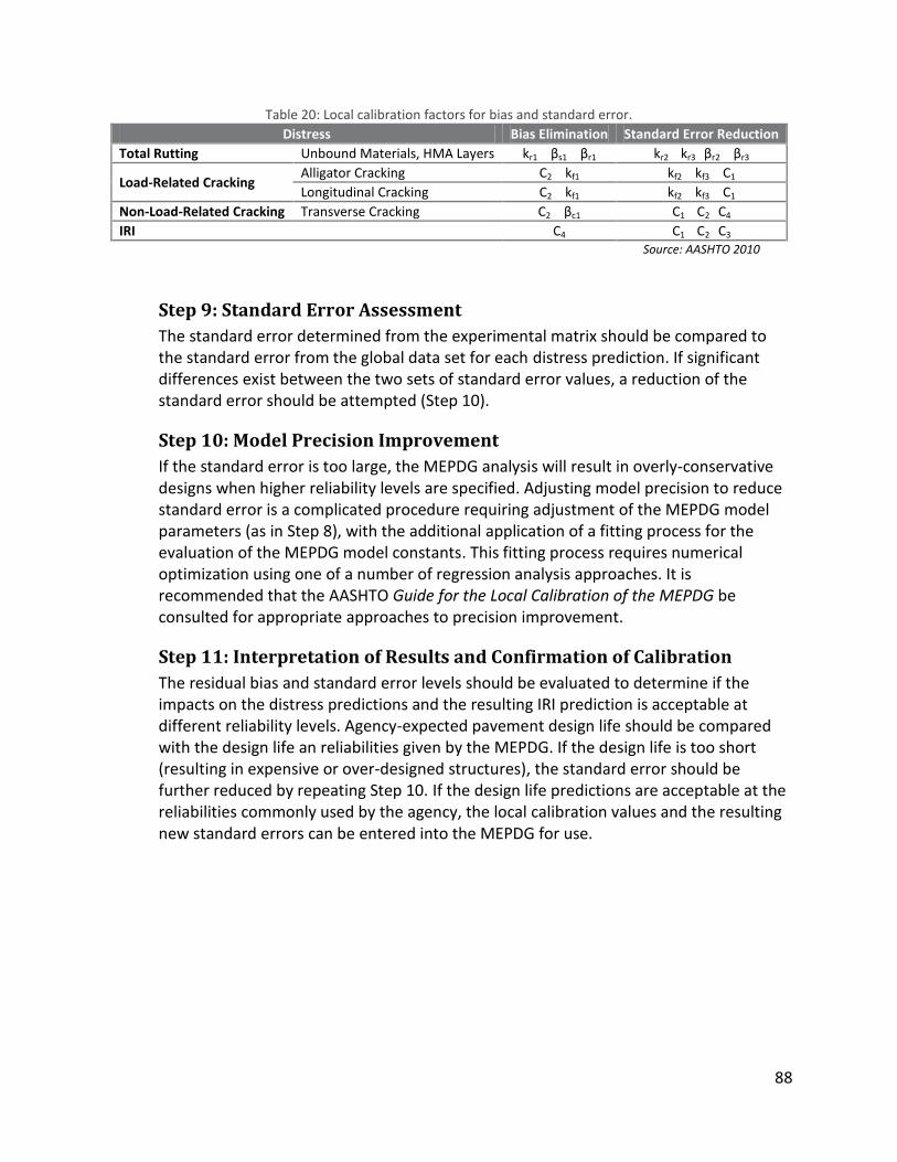
88

Table 20: Local calibration factors for bias and standard error.

Distress Bias Elimination Standard Error Reduction

Total Rutting Unbound Materials, HMA Layers kr1 βs1 βr1 kr2 kr3 βr2 βr3

Load-Related Cracking Alligator Cracking C2 kf1 kf2 kf3 C1

Longitudinal Cracking C2 kf1 kf2 kf3 C1

Non-Load-Related Cracking Transverse Cracking C2 βc1 C1 C2 C4

IRI C4 C1 C2 C3

Source: AASHTO 2010

Step 9: Standard Error Assessment

The standard error determined from the experimental matrix should be compared to the standard error from the global data set for each distress prediction. If significant differences exist between the two sets of standard error values, a reduction of the standard error should be attempted (Step 10).

Step 10: Model Precision Improvement

If the standard error is too large, the MEPDG analysis will result in overly-conservative designs when higher reliability levels are specified. Adjusting model precision to reduce standard error is a complicated procedure requiring adjustment of the MEPDG model parameters (as in Step 8), with the additional application of a fitting process for the evaluation of the MEPDG model constants. This fitting process requires numerical optimization using one of a number of regression analysis approaches. It is recommended that the AASHTO Guide for the Local Calibration of the MEPDG be consulted for appropriate approaches to precision improvement.

Step 11: Interpretation of Results and Confirmation of Calibration

The residual bias and standard error levels should be evaluated to determine if the impacts on the distress predictions and the resulting IRI prediction is acceptable at different reliability levels. Agency-expected pavement design life should be compared with the design life an reliabilities given by the MEPDG. If the design life is too short (resulting in expensive or over-designed structures), the standard error should be further reduced by repeating Step 10. If the design life predictions are acceptable at the reliabilities commonly used by the agency, the local calibration values and the resulting new standard errors can be entered into the MEPDG for use.

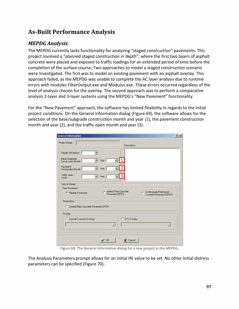
89

As-Built Performance Analysis

MEPDG Analysis

The MEPDG currently lacks functionality for analyzing “staged construction” pavements. This project involved a “planned staged construction in depth”, where the first two layers of asphalt concrete were placed and exposed to traffic loadings for an extended period of time before the completion of the surface course. Two approaches to model a staged construction scenario were investigated. The first was to model an existing pavement with an asphalt overlay. This approach failed, as the MEPDG was unable to complete the AC layer analysis due to runtime errors with modules FilterOutput.exe and Modulus.exe. These errors occurred regardless of the level of analysis chosen for the overlay. The second approach was to perform a comparative analysis 2-layer and 3-layer systems using the MEPDG’s “New Pavement” functionality. For the “New Pavement” approach, the software has limited flexibility in regards to the initial project conditions. On the General Information dialog (Figure 69), the software allows for the selection of the base/subgrade construction month and year (1), the pavement construction month and year (2), and the traffic open month and year (3).

Figure 69: The General Information dialog for a new project in the MEPDG.

The Analysis Parameters prompt allows for an initial IRI value to be set. No other initial distress parameters can be specified (Figure 70).

90

Figure 70: The Analysis Parameters dialog for a new project in the MEPDG.

Due to these limitations, three scenarios were investigated (Table 21). The first (Scenario A) assumed that the entire pavement section had been completed prior to the Traffic Open Date of April 2010; that a staged construction scenario never occurred. Scenario B modeled a 2-layer system, assuming that the wearing course was never completed. Scenario C represents the closest approximation of the actual site conditions: the terminal IRI for the 2-layer system as of October 2011 was used as the initial IRI for a 3-layer analysis starting in October 2011. This involved performing the 2-layer analysis from April 2010 to October 2011 and using the resulting Terminal IRI value to “seed” the new analysis, which was modeled from October 2011 onward.

Table 21: Summary of Scenario conditions used in the comparative analysis.

Scenario Description Subgrade Pavement Open Date

A 3-Layer (Complete) Structure 10/2009 11/2009 04/2010

B 2-Layer (Incomplete) Structure 10/2009 11/2009 04/2010

C1 2-Layer (April 2010 to October 2011) 10/2009 11/2009 04/2010

C2 3-Layer (Initial IRI Increased) 10/2009 10/2011 10/2011

91

Figure 71: IRI over 10-year analysis period, all as-built scenarios.

A ten year analysis period was sufficient to see the performance differences between the scenarios. Although scenarios A and B appear to be identical after the initial divergence in the first few months, the separation in IRI between them continues to increase, with the 2-layer structure exhibiting the expected poorer performance (Figure 72). Scenario C, which is the 3-layer with the increased initial IRI, performs worse than the previous scenarios.

Figure 72: The difference in IRI between Scenario A and Scenario B over the 10-year analysis period.

This poor performance may be due to the MEPDG’s internal handling of IRI calculations, similar to the erratic increases seen in the monthly IRI predictions for the Level 1 analyses performed in Section 0However, IRI is not a good indicator of pavement performance, given the MEPDG’s inherent limitations for modeling pre-existing conditions or staged construction scenarios.

65

70

75

80

85

90

95

0 12 24 36 48 60 72 84 96 108 120

IRI (

in/m

i)

Design Month

Scenario A Scenario B Scenario C

Wearing Course

Wearing Course Completed

0.00

0.50

1.00

1.50

2.00

2.50

3.00

0 12 24 36 48 60 72 84 96 108 120

IRI D

iffe

ren

ce (

in/m

i)

Design Month

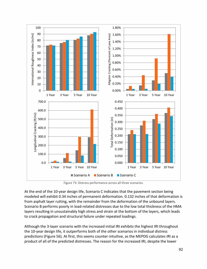
92

Figure 73: Distress performance across all three scenarios.

At the end of the 10-year design life, Scenario C indicates that the pavement section being modeled will exhibit 0.34 inches of permanent deformation. 0.132 inches of that deformation is from asphalt layer rutting, with the remainder from the deformation of the unbound layers. Scenario B performs poorly in load-related distresses due to the low total thickness of the HMA layers resulting in unsustainably high stress and strain at the bottom of the layers, which leads to crack propagation and structural failure under repeated loadings. Although the 3-layer scenario with the increased initial IRI exhibits the highest IRI throughout the 10-year design life, it outperforms both of the other scenarios in individual distress predictions (Figure 56). At first, this seems counter-intuitive, as the MEPDG calculates IRI as a product of all of the predicted distresses. The reason for the increased IRI, despite the lower

0

10

20

30

40

50

60

70

80

90

100

1 Year 3 Year 5 Year 10 Year

Inte

rnat

ion

al R

ou

ghn

ess

Ind

ex (

in/m

i)

0.00%

0.20%

0.40%

0.60%

0.80%

1.00%

1.20%

1.40%

1.60%

1.80%

1 Year 3 Year 5 Year 10 Year

Alli

gato

r C

rack

ing

(Per

ecen

t o

f La

ne

Are

a)

0.0

100.0

200.0

300.0

400.0

500.0

600.0

700.0

1 Year 3 Year 5 Year 10 Year

Lon

gitu

din

al C

rack

ing

(ft/

mi)

0.000

0.050

0.100

0.150

0.200

0.250

0.300

0.350

0.400

0.450

1 Year 3 Year 5 Year 10 Year

Tota

l Def

orm

atio

n (

in)

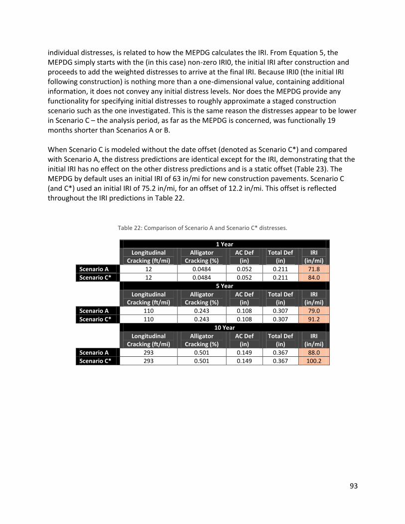
93

individual distresses, is related to how the MEPDG calculates the IRI. From Equation 5, the MEPDG simply starts with the (in this case) non-zero IRI0, the initial IRI after construction and proceeds to add the weighted distresses to arrive at the final IRI. Because IRI0 (the initial IRI following construction) is nothing more than a one-dimensional value, containing additional information, it does not convey any initial distress levels. Nor does the MEPDG provide any functionality for specifying initial distresses to roughly approximate a staged construction scenario such as the one investigated. This is the same reason the distresses appear to be lower in Scenario C – the analysis period, as far as the MEPDG is concerned, was functionally 19 months shorter than Scenarios A or B. When Scenario C is modeled without the date offset (denoted as Scenario C*) and compared with Scenario A, the distress predictions are identical except for the IRI, demonstrating that the initial IRI has no effect on the other distress predictions and is a static offset (Table 23). The MEPDG by default uses an initial IRI of 63 in/mi for new construction pavements. Scenario C (and C*) used an initial IRI of 75.2 in/mi, for an offset of 12.2 in/mi. This offset is reflected throughout the IRI predictions in Table 22.

Table 22: Comparison of Scenario A and Scenario C* distresses.

1 Year

Longitudinal Cracking (ft/mi)

Alligator Cracking (%)

AC Def (in)

Total Def (in)

IRI (in/mi)

Scenario A 12 0.0484 0.052 0.211 71.8

Scenario C* 12 0.0484 0.052 0.211 84.0

5 Year

Longitudinal Cracking (ft/mi)

Alligator Cracking (%)

AC Def (in)

Total Def (in)

IRI (in/mi)

Scenario A 110 0.243 0.108 0.307 79.0

Scenario C* 110 0.243 0.108 0.307 91.2

10 Year

Longitudinal Cracking (ft/mi)

Alligator Cracking (%)

AC Def (in)

Total Def (in)

IRI (in/mi)

Scenario A 293 0.501 0.149 0.367 88.0

Scenario C* 293 0.501 0.149 0.367 100.2

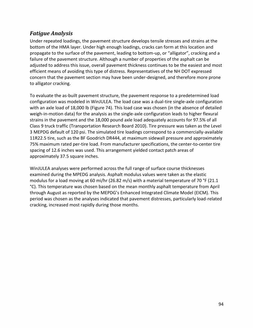
94

Fatigue Analysis

Under repeated loadings, the pavement structure develops tensile stresses and strains at the bottom of the HMA layer. Under high enough loadings, cracks can form at this location and propagate to the surface of the pavement, leading to bottom-up, or “alligator”, cracking and a failure of the pavement structure. Although a number of properties of the asphalt can be adjusted to address this issue, overall pavement thickness continues to be the easiest and most efficient means of avoiding this type of distress. Representatives of the NH DOT expressed concern that the pavement section may have been under-designed, and therefore more prone to alligator cracking. To evaluate the as-built pavement structure, the pavement response to a predetermined load configuration was modeled in WinJULEA. The load case was a dual-tire single-axle configuration with an axle load of 18,000 lb (Figure 74). This load case was chosen (in the absence of detailed weigh-in-motion data) for the analysis as the single-axle configuration leads to higher flexural strains in the pavement and the 18,000 pound axle load adequately accounts for 97.5% of all Class 9 truck traffic (Transportation Research Board 2010). Tire pressure was taken as the Level 3 MEPDG default of 120 psi. The simulated tire loadings correspond to a commercially-available 11R22.5 tire, such as the BF Goodrich DR444, at maximum sidewall pressure and approximately 75% maximum rated per-tire load. From manufacturer specifications, the center-to-center tire spacing of 12.6 inches was used. This arrangement yielded contact patch areas of approximately 37.5 square inches. WinJULEA analyses were performed across the full range of surface course thicknesses examined during the MPEDG analysis. Asphalt modulus values were taken as the elastic modulus for a load moving at 60 mi/hr (26.82 m/s) with a material temperature of 70 °F (21.1 °C). This temperature was chosen based on the mean monthly asphalt temperature from April through August as reported by the MEPDG’s Enhanced Integrated Climate Model (EICM). This period was chosen as the analyses indicated that pavement distresses, particularly load-related cracking, increased most rapidly during those months.

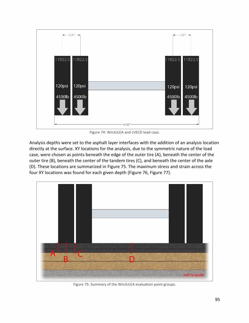
95

Figure 74: WinJULEA and LVECD load case.

Analysis depths were set to the asphalt layer interfaces with the addition of an analysis location directly at the surface. XY locations for the analysis, due to the symmetric nature of the load case, were chosen as points beneath the edge of the outer tire (A), beneath the center of the outer tire (B), beneath the center of the tandem tires (C), and beneath the center of the axle (D). These locations are summarized in Figure 75. The maximum stress and strain across the four XY locations was found for each given depth (Figure 76, Figure 77).

Figure 75: Summary of the WinJULEA evaluation point groups.

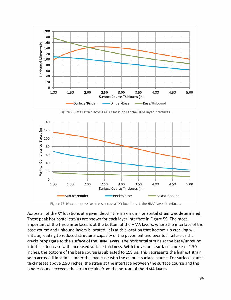
96

Figure 76: Max strain across all XY locations at the HMA layer interfaces.

Figure 77: Max compressive stress across all XY locations at the HMA layer interfaces.

Across all of the XY locations at a given depth, the maximum horizontal strain was determined. These peak horizontal strains are shown for each layer interface in Figure 59. The most important of the three interfaces is at the bottom of the HMA layers, where the interface of the base course and unbound layers is located. It is at this location that bottom-up cracking will initiate, leading to reduced structural capacity of the pavement and eventual failure as the cracks propagate to the surface of the HMA layers. The horizontal strains at the base/unbound interface decrease with increased surface thickness. With the as-built surface course of 1.50 inches, the bottom of the base course is subjected to 159 με. This represents the highest strain seen across all locations under the load case with the as-built surface course. For surface course thicknesses above 2.50 inches, the strain at the interface between the surface course and the binder course exceeds the strain results from the bottom of the HMA layers.

0

20

40

60

80

100

120

140

160

180

200

1.00 1.50 2.00 2.50 3.00 3.50 4.00 4.50 5.00

Ho

rizo

nta

l Mic

rost

rain

Surface Course Thickness (in)

Surface/Binder Binder/Base Base/Unbound

0

20

40

60

80

100

120

140

1.00 1.50 2.00 2.50 3.00 3.50 4.00 4.50 5.00

Ver

tica

l Co

mp

ress

ive

Str

ess

(psi

)

Surface Course Thickness (in)

Surface/Binder Binder/Base Base/Unbound

97

The stresses and strains reported by WinJULEA were corroborated by an LVECD analysis performed at North Carolina State University. The results were passed to ALPHA-Fatigue in order to estimate the cycles until failure (Nf) for the pavement structure. ALPHA-Fatigue (Asphalt Pavement Hierarchical Analysis-Fatigue) is a software program used to evaluate the linear viscoelastic/VECD parameters of an asphalt mix using inputs from the Asphalt Mixture Performance Tester (AMPT). From the characterization of the asphalt mixes in ALPHA-Fatigue, it is possible to evaluation load cycles until failure given specified levels of strain. It is worth noting that the MEPDG does not consider the Fatigue Endurance Limit concept (FEL) in its modeling or analysis. FEL is the strain threshold below which no cumulative damage occurs within the HMA structure, regardless of the number of load cycles. Theoretically, this states that if a pavement structure can be designed such that the strains at the bottom of the HMA layers is low enough, the pavement should never experience a structural failure due to traffic loadings. The FEL threshold was originally proposed as 70 µε by Monismith and McLean, a value which found support in further studies (Transportation Research Board 2010). Although research suggests that the exact FEL is mixture-dependent and that the value proposed by Monismith and McLean was conservative, the relationship of asphalt strain to cycles-until-failure exhibits an asymptotic relationship as it approaches 70 µε, indicating that for practical purposes, material variability has little effect at that level of repeated traffic loading (Carpenter, Ghuzlan and Shen 2003, Willis 2009). NCAT laboratory testing of various mixtures lead to the establishment of a new threshold that reflected the mixture-dependent nature of the FEL. The research defined the new limit as the strain required to produce a failure after 50 million load cycles (Transportation Research Board 2010). With the base and binder course thicknesses unchanged, only varying the surface course thickness, the strain at the bottom of the HMA layers fails to reach this threshold value even at thicknesses beyond 4.50 inches – a total HMA thickness exceeding 9.125 inches (Figure 78).

Figure 78: Stress and Strain at the bottom of the HMA layers for various surface course thicknesses.

50

70

90

110

130

150

170

190

50

70

90

110

130

150

170

190

1.00 1.50 2.00 2.50 3.00 3.50 4.00 4.50 5.00

Ten

sile

Mic

rost

rain

Ten

sile

Str

ess

(psi

)

Surface Course Thickness (in) Tensile Stress Tensile Microstrain

98

However, when compared with the MEPDG traffic modeling, ALPHA results indicate that it may not be necessary to design for such a low strain threshold to achieve a practical service life with the pavement structure under consideration. For the given pavement structure, with a surface course thickness of 1.50 inches, WinJULEA calculated 159 µε at the bottom of the HMA layers, resulting in an ALPHA prediction Nf of 2,600,484 cycles. From the MEPDG traffic growth model, this places the fatigue limit around 120 months (10 years) of service (Figure 79). Following the MEPDG cumulative truck values, to achieve a 20-year structural life, the surface course would have to be increased only 0.50 inches (Figure 80). Doing so reduces the predicted strain at the base of the HMA layers from 159 µε to 106 µε (Figure 78). The MEPDG truck traffic volumes used for this analysis were based upon the best available information and assumptions of growth factors that may not accurately represent the true traffic volumes at the site, particularly as time goes on. Investigation of the stresses and strains predicted by ALPHA-Fatigue at the interfaces of the HMA layers reveals that the surface and binder courses may not be subjected to deleterious stress and strain (Figure 81, Figure 82). ALPHA modeling indicated that under the worst-case surface course thickness scenarios, both HMA layers would exceed Nf values of 10 million and 12 million cycles, respectively (more than 36 and 42 years, by MEPDG traffic model predictions). As-built, the surface course experiences a maximum of 10 tensile microstrain and 3.45 psi in tensile stress. The binder course experiences a maximum of 42.1 tensile microstrain and 6.37 psi in tensile stress.

Figure 79: ALPHA-Fatigue pavement life prediction versus MPEDG traffic model.

Ye

ar 1

0

2.6m Loadings

0.0E+00

1.0E+06

2.0E+06

3.0E+06

4.0E+06

5.0E+06

6.0E+06

0 1 2 3 4 5 6 7 8 9 10 11 12 13 14 15 16 17 18 19 20

MEP

DG

Cu

mu

lati

ve T

ruck

Tra

ffic

MEPDG Analysis Year

99

Figure 80: Resulting Nf increase from changing the surface course from 1.50 to 2.00 inches.

Figure 81: Tensile stress levels at the lower interfaces of each of the three HMA layers.

0.00E+00

1.00E+06

2.00E+06

3.00E+06

4.00E+06

5.00E+06

6.00E+06

7.00E+06

8.00E+06

9.00E+06

1.00E+07

1.00 1.25 1.50 1.75 2.00 2.25 2.50 2.75 3.00

Cyc

les

Un

til F

ailu

re (

Nf)

Surface Course Thickness (in)

0

20

40

60

80

100

120

140

160

180

200

1.00 1.50 2.00 2.50 3.00 3.50 4.00 4.50 5.00

Ten

sile

Str

ess

(psi

)

Surface Course Thickness (in)

Bottom of Base Course Bottom of Binder Course Bottom of Surface Course

100

Figure 82: Tensile microstrain levels at the lower interfaces of each of the three HMA layers.

Due to the staged construction that the pavement section underwent, it is important to also consider the pre-completion two-layer structure in a fatigue analysis in an attempt to determine if the pavement experienced strain levels high enough to cause permanent damage to the structure. Here, the 18,000lb single tandem axle load case was used to evaluate the 2-layer structure (Table 23), prior to the completion of the surface course. The results were compared to the completed 3-layer structure (Table 24). These two tables summarize the maximum stresses and strains for each depth at all of the XY locations analyzed.

Table 23: WinJULEA 2-Layer analysis results, max across all XY locations.

Z (in) X (in) Y (in) σX (psi) σY (psi) σZ (psi)

μεX (in/in)

μεY (in/in)

μεZ (in/in)

ΔZ (in)

Surf

ace

0.10 0.00 0.00 224.00 197.00 125.00 190.00 128.00 -38.30 0.0116

0.10 0.00 6.30 123.00 56.20 2.95 176.00 20.60 -103.00 0.0115

0.10 0.00 12.60 225.00 195.00 125.00 194.00 123.00 -37.00 0.0118

0.10 0.00 51.00 2.99 -6.39 -0.09 9.01 -12.70 1.89 0.0039

Bin

der

/ B

ase 1.99 0.00 0.00 38.40 35.40 86.30 -7.18 -14.20 104.00 0.0116

1.99 0.00 6.30 21.00 31.30 5.25 14.10 37.90 -22.40 0.0117

1.99 0.00 12.60 38.50 35.30 86.30 -7.01 -14.30 104.00 0.0118

1.99 0.00 51.00 2.36 -0.56 -0.03 4.40 -2.37 -1.13 0.0039

Bas

e/

Sub

grad

e 4.62 0.00 0.00 -159.00 -131.00 20.20 -215.00 -148.00 218.00 0.0113

4.62 0.00 6.30 -112.00 -31.60 15.80 -191.00 3.91 118.00 0.0115

4.62 0.00 12.60 -159.00 -131.00 20.20 -215.00 -147.00 217.00 0.0114

4.62 0.00 51.00 1.39 6.99 -0.04 -1.86 11.70 -5.32 0.0039

Key: Tension Compression

0

20

40

60

80

100

120

140

160

180

200

1.00 1.50 2.00 2.50 3.00 3.50 4.00 4.50 5.00

Ten

sile

Mic

rost

rain

Surface Course Thickness (in)

Bottom of Base Course Bottom of Binder Course Bottom of Surface Course

101

Table 24: WinJULEA 3-Layer analysis results, max across all XY locations.

Z (in) X (in) Y (in) σX (psi) σY (psi) σZ (psi)

μεX (in/in)

μεY (in/in)

μεZ (in/in)

ΔZ (in) Su

rfac

e 0.10 0.00 0.00 156.00 140.00 121.00 157.00 106.00 42.20 0.0103

0.10 0.00 6.30 77.80 44.60 1.76 150.00 40.90 -100.00 0.0100

0.10 0.00 12.60 157.00 138.00 121.00 162.00 99.00 44.10 0.0105

0.10 0.00 51.00 2.18 -6.62 -0.06 11.00 -18.00 3.65 0.0040

Wea

rin

g/

Bin

der

1.49 0.00 0.00 85.70 77.60 109.00 49.70 23.20 127.00 0.0102

1.49 0.00 6.30 42.70 38.50 1.36 70.10 56.40 -66.10 0.0102

1.49 0.00 12.60 85.70 77.50 109.00 49.90 22.90 127.00 0.0104

1.49 0.00 51.00 1.82 -3.45 0.00 7.39 -9.97 1.38 0.0040

Bin

der

/

Bas

e

3.49 0.00 0.00 -4.07 -1.06 59.60 -42.10 -35.20 105.00 0.0100

3.49 0.00 6.30 -6.37 14.20 8.98 -24.80 22.80 10.70 0.0102

3.49 0.00 12.60 -4.01 -1.04 59.60 -42.00 -35.20 105.00 0.0102

3.49 0.00 51.00 1.81 1.42 0.00 2.25 1.35 -1.94 0.0040

Bas

e/

Sub

grad

e 6.12 0.00 0.00 -117.00 -95.30 14.40 -159.00 -106.00 159.00 0.0097

6.12 0.00 6.30 -95.70 -43.70 12.50 -152.00 -26.20 110.00 0.0101

6.12 0.00 12.60 -117.00 -95.10 14.40 -159.00 -106.00 159.00 0.0099

6.12 0.00 51.00 0.77 9.22 0.03 -4.41 16.00 -6.19 0.0040

Key: Tension Compression

As expected, the 2-layer system undergoes greater deformation and is exposed to higher strains. At the surface, peak tensile strain is approximately 3% greater in the 2-layer system. At the interface of the binder course and the base course, the tensile strain in the 2-layer system is lower, due to the decreased depth of that location relative to the surface of the pavement. This reduced asphalt thickness has a great effect on the strain at the bottom of the base course, however, increasing the peak microstrain from 159με to 215με. At these increased strains, ALPHA indicates an Nf of approximately 134,600 load cycles before the base course begins to experience structural fatigue failure. From the MEPDG traffic volumes, the 2-layer pavement would reach the cycle limit between 6 and 7 months from the traffic open date. The actual staged construction timeline exposed the 2-layer system to traffic loading from 04/2010 to 10/2011, or approximately 18 months and 360,000 load cycles. It should be noted that this represents the worst-case scenario, as it is unlikely that the pavement section actually experienced that level of truck traffic, due to traffic pattern changes and other events occurring at the project site leading up to the completion of the surface course. The fatigue analysis, including the stress and strain modeling done with WinJULEA and the LVECD, was performed assuming a single reference temperature of 70 °F (21.1 °C). This results in a limited evaluation of the HMA layers, as it only models the structure under one set of stiffness and asphalt properties.

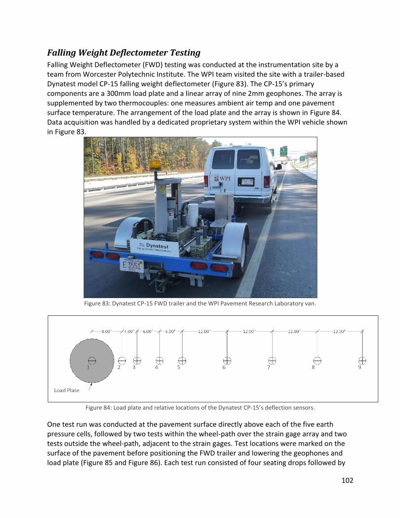
102

Falling Weight Deflectometer Testing

Falling Weight Deflectometer (FWD) testing was conducted at the instrumentation site by a team from Worcester Polytechnic Institute. The WPI team visited the site with a trailer-based Dynatest model CP-15 falling weight deflectometer (Figure 83). The CP-15’s primary components are a 300mm load plate and a linear array of nine 2mm geophones. The array is supplemented by two thermocouples: one measures ambient air temp and one pavement surface temperature. The arrangement of the load plate and the array is shown in Figure 84. Data acquisition was handled by a dedicated proprietary system within the WPI vehicle shown in Figure 83.

Figure 83: Dynatest CP-15 FWD trailer and the WPI Pavement Research Laboratory van.

Figure 84: Load plate and relative locations of the Dynatest CP-15’s deflection sensors.

One test run was conducted at the pavement surface directly above each of the five earth pressure cells, followed by two tests within the wheel-path over the strain gage array and two tests outside the wheel-path, adjacent to the strain gages. Test locations were marked on the surface of the pavement before positioning the FWD trailer and lowering the geophones and load plate (Figure 85 and Figure 86). Each test run consisted of four seating drops followed by

103

twelve calibrated test drops. Seating drops are performed to eliminate errors due to surface irregularities or loose debris at the location of the geophones and to ensure that the load plate is in adequate contact with the pavement surface before the calibrated test drops are performed (Federal Highway Administration 2011).

Figure 85: The CP-15 FWD being positioned over the location of subsurface instrumentation.

Figure 86: The CP-15 load plate being positioned over a pre-determined wheelpath testing location.

104

The location of each of the tests is shown in Figure 87. The recorded data indicated that the pressure cells were functional, however, no data was collected from the strain gages. It was discovered after testing was complete, that none of the strain gage signals had registered. All of the strain channels had zero readings. This does not necessarily indicate malfunction or failure of the strain gages, as even damaged or “open” gages would typically result in background noise in the channel. Null readings could indicate that the fault lies within the portable DAQ or its modules. Asphalt strain gages placed within the pavement section are exposed to loadings during the construction phases, and despite designed to be fairly robust, often have relatively low survivability rates compared with other in-pavement instrumentation (Timm, Priest and McEwan 2004). Survival rates between 40% and 60%, and as low as 25%, were seen at the NCAT test track, whose instrumentation plan was used as the basis for this project (Timm 2009, Steele 2010).

Figure 87: The locations of the FWD tests, in sequence.

105

Summary and Conclusions Project 14282S saw the completion of the weather station and pavement instrumentation and the final phases of material testing in late 2011. The final MEPDG analysis runs were completed in the winter of 2012. Planned project delays (staged construction) affected the functionality and survivability of the in-pavement instrumentation, notably the strain gages and the axle sensor strip loop wires. The instrumentation package was augmented by an upstream weigh-in-motion station which ameliorated the need for a functional three axle sensor array. The weigh-in-motion station at the site will provide a more accurate picture of traffic volume, wheel wander, and axle load spectra than what was available at the time of writing, which will allow for a higher-level MEPDG analysis as far as traffic data is concerned. WinJULEA strain analyses, coupled with ALPHA Fatigue predictions, indicate that the completed pavement structure is not under-designed. The analysis indicates a limit of approximately 2.6 million cycles until structural failure occurs within the pavement section, most likely at the bottom of the base layer of asphalt concrete. From the MEPDG traffic model, 2.6 million cycles provides a service life of approximately 120 months (10 years). Calibration of the MEPDG coupled with distress observations at the site will further refine this prediction. The fatigue analysis performed on the incomplete (staged-construction) pavement Despite modeling limitations present in the MEPDG, an analysis of the as-built pavement section using the gathered materials and traffic data indicates that it will exceed the distress performance limits set by the NHDOT. The resulting service life should be great enough to allow for sufficient distress data to be collected in order to begin a calibration of the MEPDG. It is worth noting that due to the staged construction and MEPDG’s inability to adequately model that type of scenario, that determination of proper calibration factors may be difficult.

106

Future Work

Instrumentation

While the pressure cells and related data acquisition is functional, several tasks need to be undertaken to utilize the full capabilities of the site instrumentation:

1. The strain gages will need additional troubleshooting to determine the cause of the issues with data collection.

2. The axle sensor strip array will require either lead wire repair or simultaneous data collection from the WIMS in order to determine vehicle velocity and wheel-wander during testing.

Calibration

In order to refine the MEPDG analysis of the pavement section and improve the accuracy of the distress predictions for the as-built structure, it will be necessary to calibrate the MEPDG through a two-pronged approach: continued refinement of the climatic data and the truck traffic and continued distress observations followed by adjustment of the calibration factors for the various distresses, in order to reduce bias and the standard error of the estimate. The calibration process can be broken into three main tasks:

1. Refine the traffic inputs with data from the weigh-in-motion station located at the project site.

2. Collect environmental data from the on-site weather station and use that data to develop a site-specific climactic file with the MEPDG’s EICM.

3. Collect periodic distress observations at the site and compare those to the predicted distresses from the MEPDG to develop local calibration factors by undertaking the AASHTO-recommended calibration procedures to reduce the bias and standard error of the estimate in the MEPDG results.

The local calibration process is discussed in greater detail on pages 84-88 of this report. Further documentation, with supporting examples, can be found in the AASHTO Guide for the Local Calibration of the Mechanistic-Empirical Pavement Design Guide.

Cost-to-Benefit Analysis From the results of the MEPDG analyses performed during this project, it is apparent that certain Level 1 inputs may have much greater effect on the distress predictions than others, specifically traffic inputs and asphalt material properties. It is recommended that additional work be done to evaluate the cost of improving inputs compared with the effect they have on the accuracy of the MEPDG predictions. A cost/benefit analysis would serve to inform allocation decisions on projects where resources are limited. In scenarios where the roadway is over-designed (the distress thresholds are significantly high, relative to the distresses predicted by an experience-based evaluation), it may not be necessary to pursue Level 1 inputs, as the increase in accuracy would not result in a change to the proposed design.

107

Works Cited AASHTO. AASHTO Guide for Design of Pavement Structures, 1993. Washington, DC: American

Association of State Highway and Transportation Officials, 1993. —. Guide for the Local Calibration of the Mechanistic-Empirical Pavement Design Guide. Washington,

D.C.: American Association of State Highway and Transportation Officials, 2010. —. M-E Design: Implementation of a Mechanistic-Empirical Pavement Design. Washington, DC: AASHTO,

2003. —. Mechanistic-Empirical Pavement Design Guide: A Manual of Practice. Washington, D.C.: American

Association of State Highway and Transportation Officials, 2008. Applied Research Associates, Inc. M-EPDG: Mechanistic-Empirical Pavement Design Guide. 2007. Bollinger, Robert E. "Email to Justin Lowe." December 12, 2011. BP p.l.c. BP Statistical Review of World Energy. Economic Report, London, UK: BP, 2011. Burton Jr., G. Allen, and Robert Pitt. Stormwater Effects Handbook. Boca Raton: CRC Press, 2002. Campbell Scientific, Inc. Application Note 4-S: Weather Station Siting and Installation Tools.

Memorandum, Campbell Scientific, Inc., 1997. Carpenter, Samuel H, Khalid A Ghuzlan, and Shihui Shen. A Fatigue Endurance Limit for Highways and

Airport Pavements. Transportation Research Board, 2003. Clark, Corey J. Comparing the stiffness and strength of natural aggregate to building derived aggregate.

M.S. Thesis, Durham: University of New Hampshire, 2010. Corti, James, interview by Justin Lowe. Phone call (August 16, 2011). Cross, Steve, and Zahid Hossain. Development of Flexible Pavement Database for Local Calibration of

MEPDG. Annual Report, Oklahoma City, OK: Oklahoma Department of Transportation, 2009. Daniel, J S, and G R Chehab. "Use of RAP Mixtures in the Mechanistic Empirical Pavement Design Guide."

Transportation Research Board 87th Annual Meeting. Washington, DC, 2008. Daniel, J S, and Y Richard Kim. "Development of a simplified fatigue test and analysis procedure using a

viscoelastic continuum damage model." Journal of the Association of Asphalt Paving Technologists 71 (2002): 619-650.

Dzotepe, George, and Khaled Ksaibati. MPC Report No. 10-225A: Implementation of the Mechanistic-Empirical Pavement Design Guide (MEPDG). Laramie, WY: University of Wyoming, 2010.

Eslaminia, Mehran, Senganal Thirunavukkarasu, Murthy N Guddati, and Y Richard Kim. "Accelerated Pavement Performance Modeling Using Layered Viscoelastic Analysis." 7th RILEM International Conference on Cracking in Pavements. Heidelberg: Springer Netherlands, 2012. 497-506.

Falola, Toyin, and Ann Genova. The Politics of the Global Oil Industry: An Introduction. Wesport, CT: Greenwood Publishing Group, 2005.

Federal Highway Administration. Falling Weight Deflectometer Calibration Center and Operational Improvements: Redevelopment of The Calibration Protocol and Equipment. LTPP Publication, Federal Highway Administration, US Department of Transportation, Washington, DC: US Department of Transportation, 2011.

Fwa, T F. The Handbook Of Highway Engineering. Boca Raton: CRC Press, 2006. Goodman, S N. "Assessing variability of surface distress surveys in Canadian Long-Term Pavement

Performance Program." Transportation Research Record, no. 1764 (2001): 112-118. Herbert, Abraham. Asphalts and allied substances: their occurrence, modes of production, uses in the

arts and methods of testing. 2. New York: D. Van Nostrand Company, Inc., 1920. Huang, Yang H. Pavement Analysis and Design. 2nd. Upper Saddle River, New Jersey: Pearson Prentice

Hall, 2004. Ingalls, Walter Renton. The Mineral Industry: It's Statististics, Technology, and Trade. Vol. 14. New York:

The Engineering and Mining Journal, 1906.

108

Jones, D S J, and Peter R Pujadó. Handbook of Petroleum Processing. Dordrecht, Netherlands: Springer, 2006.

Journal of the Western Society of Engineers. Vol. 27. Chicago: Western Society of Engineers, 1922. Khazanovich, L, S F Wojtkiewicz, and R Velasquez. "MEPDG-RED: A Framework for Reliability Analysis

with the Mechanistic Empirical Pavement Design Procedure." Transportation Research Board 87th Annual Meeting. Washington, DC, 2008.

Kile, Joseph, interview by US Senate Committee on Finance. Testimony, Statement on the Highway Trust Fund and Paying for Highways (May 17, 2011).

Li, Jianhua, Jeff S Uhlmeyer, Joe P Mahoney, and Stephen T Muench. Use of the 1993 AASHTO Guide, MEPDG, and Historical Performance to Update the WSDOT Pavement Design Catalog. Research Report, Washington State Department of Transportation, Olympia, WA: Washington State Department of Transportation, 2011.

Mun, Sungho, Murthy N Guddati, and Y Richard Kim. "Viscoelastic Continuum Damage Finite Element Modeling of Asphalt Pavements for Fatigue Cracking Evaluation." KSCE Journal of Civil Engineering, 2006: 97-104.

Muthadi, N R, and Y R Kim. "Local Calibration of the MEPDG for Flexible Pavement Design." Transportation Research Board 87th Annual Meeting. Washington, DC, 2008.

NCHRP. "Changes to the Mechanistic-Empirical Pavement Design Guide Software Through Version 0.900." In NCHRP Results Digest 308, by Nactional Cooperative Highway Research Program. Washington, DC: Transportation Research Board of the National Academies, 2006.

Osman, Ali. Evaluation of the Mechanistic Empirical Pavement Design Guide (NCHRP 1-37A). Review, Ottawa: Institute de recherche en construction (Conceil national de recherches Canada), 2005.

Perera, R W, S D Kohn, and G R Rada. LTPP Manual for Profile MEasurements: Operational Field Guidelines, Version 4. Technical Report, Washington, DC: Federal Highway Administration, 2002.

Rabab'ah, S, and R Y Liang. "Evaluation Of Mechanistic Empirical Design Approach Over Permeable Base Materials." Transportation Research Board 87th Annual Meeting 2008. Washington, DC: Gannett Fleming, Inc., 2007.

Rada, G R, C L Wu, R K Bhandari, G E Elkins, A R Shekharan, and J S Miller. Study of LTPP Distress Data Variability: Volume I. McLean, VA: Federal Highway Administration, 1999.

Schram, Scott A, and Magdy Abdelrahman. "Integration of Mechanistic–Empirical Pavement Design Guide distresses with local performance indices." Transportation Research Record: Journal of the Transportation Research Board, no. 2153 (2010): 13-23.

Schwartz, Charles W, and Regis L Carvalho. Implementation of the NCHRP 1-37A Design Guide, Volume 2: Evaluation of Mechanistic-Empirical Design Procedure. Final Report, College Park, Maryland: University of Maryland Department of Civil and Environmental Engineering, 2007.

Selezneva, Olga I. Development of Mechanistic-Empirical Damage Assessment Procedures for CRC Pavements with Emphasis on Traffic Loading Characteristics. PhD Dissertation, Morgantown, WV: West Virginia University, 2002.

Sharpe, Gary W. "Distribution of the Recommended Mechanistic-Empirical Design Guide (NCHRP Project 1-37A)." Committee Correspondence Memorandum. AASHTO Joint Task Force on Pavements, June 23, 2004.

Shekharan, A R, G R Rada, G E Elkins, and W Y Bellinger. "Assessment of long-term pavement performance plan wall projection-based distress data variability." Transportation Research Record, no. 1643 (1998): 95-109.

Shirley, Chad. Economic and Budget Issue Brief: Spending and Funding for Highways. Brief, Washington, DC: US Congressional Budget Office, 2011.

State of California. CalTrans Division of Construction. February 02, 2012. http://www.dot.ca.gov/hq/construc/ (accessed February 02, 2012).

109

Steele, Matthew. Sensor Installation for the Local Calibration of the Mechanistic Empirical Pavement Design Guide in New Hampshire. M.S. Thesis, Durham: University of New Hampshire, 2010.

Swan, D, R Tardiff, J J Hajek, and D K Hein. "Development of Regional Traffic Data for the M-E Pavement Design Guide." Transportation Research Board 87th Annual Meeting. Washington, DC, 2008.

The Apshalt Institute. "Construction Leaflet No. 7: Planned Stage Construction with Full-Depth Apshalt Concrete." Paving & Surfacing (The Asphalt Institute), May 1982.

The Journal of the Engineers' Club of Philadelphia and Affiliated Societies. Vol. 38. Philadelphia: The Engineers' Club of Philadelphia, 1921.

Timm, David H. Design, Construction and Instrumentation of the 2006 Test Track Structural Study. NCAT Report 09-01, Auburn, AL: National Center for Asphalt Technology, 2009.

Timm, David H, and A L Priest. Measurement of Wheel Wander Under Live Traffic Conditions. Conference Proceedings, Trondheim, Norway: 7th International Conference on the Bearing Capacity of Roads, Railways and Airfields, 2005.

Timm, David H, and A L Priest. Wheel Wander at the NCAT Test Track. Report No. 05-02, Auburn, Alabama: National Center for Asphalt Technology at Auburn University, 2004.

Timm, David H, Angela L Priest, and Thomas V McEwan. Design and Instrumentation of the Structural Pavement Experiment at the NCAT Test Track. Auburn: National Center for Asphalt Technology, 2004.

Tindall, William. Standard history of the city of Washington from a study of the original sources. Harvard University: H.W. Crew & Co., 1914.

Transportation Research Board. NCHRP Report 646: Validating the Fatigue Endurance Limit for Hot Mix Asphalt. Washington, DC: Transportation Research Board, 2010.

US Congress. "Report No. 72, Affairs in the District of Columbia." Reports of Committees of the House of Representatives for the Second Session of the Forty-second congress. Washington, D.C.: US Congress, May 13, 1872.

Wagner, Chris. "MEPDG: Where Are We Now?" Louisiana Transportation Engineering Conference. Baton Rouge, LA: FHWA - Resource Center, February 12, 2007.

Wang, K C, Q Li, K D Hall, V Nguyen, W Gong, and Z Hou. Database Support for the New Mechanistic-Empirical Pavement Design Guide. Fayetteville: University of Arkansas, 2007.

Willis, J R. Field Based Strain Thresholds for Flexible Perpetual Pavement Design. PhD Dissertation, Alabama: Auburn University, 2009.

Xiao, D X, K Wang, and K D Hall. Matching Distress Definitions in Field and in MEPDG. Roanoke, VA. 2010.

110

Appendices

111

Asphalt Mix Reheating Procedure Heating Loose Mix

1. Heat oven to 10°C lower than the discharge temperature. 2. Remove plastic handle from the bucket of loose mix, if equipped, and place bucket in oven for

one hour with the lid on. Start preheating a second oven to compaction temperature. Remove the lid from the bucket and continue to heat the loose mix for one more hour while the second oven warms up. Be aware of the weight of the bucket and make sure the oven can support it.

3. Insert a thermocouple or a thermometer into center of bucket. Make sure center of loose mix is at least 75°C. Record the temperature.

Dividing the Loose Mix 1. Make sure all tools and pans loose mix will be divide with or into are preheated to the

appropriate compaction temperature. 2. Remove the bucket of loose mix from the oven and pour the contents into one or two large

pans. 3. The weight needed for a sample should already be determined. Place a preheated pan on a

scale and zero. 4. Remove the loose mix from the large pan using a scoop and place into the pan on the scale.

Continue to do so until enough material is in the pan to make a compacted specimen. 5. Place massed material and pan back into the oven that is heated to the compaction

temperature. 6. Repeat steps 4 and 5 until all loose mix is removed from the large pan. Each bucket has

approximately 27 kilograms of loose mix so plan accordingly. Dividing up all the loose mix should take no longer than 10 minutes.

Compacting Divided Loose Mix 1. The divided samples of loose mix will need about 30 minutes to reach compaction temperature.

Record the temperature with a thermocouple/thermometer before continuing. 2. Once heated to compaction temperature, pour the contents of the pan into a compaction

mould and compact. 3. Depending on the equipment and size of specimen it may be necessary to place material in the

mould using multiple lifts and crosshatching with a spatula. It is preferred to add material in one lift with no mixing if possible. The procedure used needs to remain consistent.

Additional Guidelines 1. Once reheated, the loose mix shall not be cooled and reheated again. 2. Loose mix shall not be reheated for more than 4 hours. 3. All specimens to be produced must be done so with loose mix that had only been reheated one

time. Additional reheating cycles may influence the general stiffness properties of the HMA, as well as potentially increase possible blending of the RAP and virgin asphalt binders.

4. Once a bucket of loose mix is heated, all material shall be used to fabricate specimens that day.

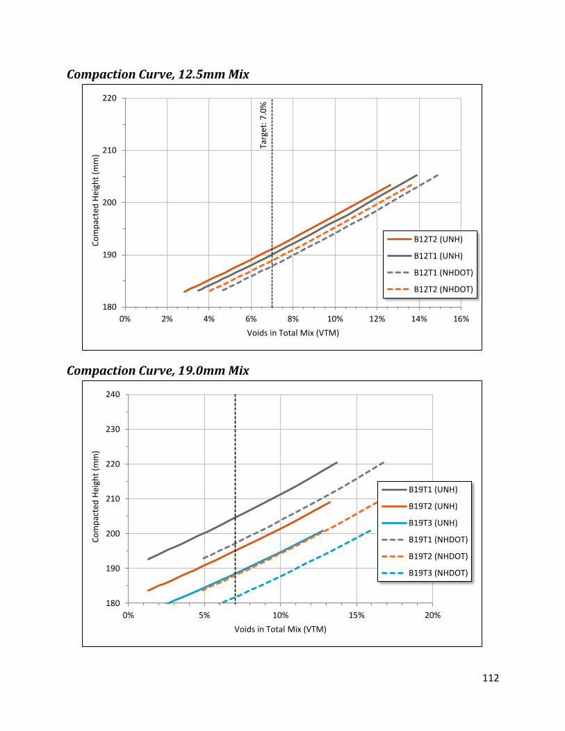
112

Compaction Curve, 12.5mm Mix

Compaction Curve, 19.0mm Mix

Targ

et:

7.0

%

180

190

200

210

220

0% 2% 4% 6% 8% 10% 12% 14% 16%

Co

mp

acte

d H

eigh

t (m

m)

Voids in Total Mix (VTM)

B12T2 (UNH)

B12T1 (UNH)

B12T1 (NHDOT)

B12T2 (NHDOT)

180

190

200

210

220

230

240

0% 5% 10% 15% 20%

Co

mp

acte

d H

eigh

t (m

m)

Voids in Total Mix (VTM)

B19T1 (UNH)

B19T2 (UNH)

B19T3 (UNH)

B19T1 (NHDOT)

B19T2 (NHDOT)

B19T3 (NHDOT)

113

Compaction Curve, 25.0mm Mix

180

190

200

210

220

0% 2% 4% 6% 8% 10% 12% 14% 16% 18%

Co

mp

acte

d H

eigh

t (m

m)

Voids in Total Mix (VTM)

B25T2 (UNH)

B25T1 (UNH)

B25T1 (NHDOT)

B25T2 (NHDOT)

114

Specific Gravity Data

NHDOT Gmb

UNH Gmb

NMSA Sample Gmb

NMSA Sample Gmb

12.5 CT-1 2.432

12.5 B12T1 2.333

12.5 CT-2 2.419

12.5 B12T2 2.317

12.5 CT-3 2.437

12.5 B1201 2.251

19.0 CB-1 2.349

12.5 B1202 2.262

19.0 CB-2 2.371

12.5 B1204 2.255

19.0 CB-3 2.281

12.5 B1205 2.261

19.0 CB-4 2.341

12.5 B1206 2.259

25.0 CBB-1 2.360

12.5 B1207 2.267

25.0 CBB-2 2.363

12.5 B1208 2.262

25.0 CBB-3 2.299

12.5 B1209 2.256

25.0 CBB-5 2.356

12.5 B1210 2.254

12.5 B1211 2.255

NHDOT Gmm

12.5 B1212 2.268

NMSA Sample Gmm

12.5 B1213 2.267

12.5 CT-1 2.292

12.5 B1214 2.243

12.5 CT-2 2.284

12.5 B1215 2.254

12.5 CT-3 2.226

12.5 B1216 2.252

19.0 CB-1 2.457

19.0 B1910 2.304

19.0 CB-2 2.455

19.0 B1911 2.329

19.0 CB-3 2.457

19.0 B1912 2.323

19.0 CB-4 2.459

19.0 B1913 2.313

25.0 CBB-1 2.462

19.0 B1914 2.335

25.0 CBB-2 2.458

19.0 B1915 2.328

25.0 CBB-3 2.459

19.0 B1916 2.336

25.0 CBB-5 2.462

19.0 B1917 2.332

25.0 B2501 2.290

25.0 B2502 2.311

25.0 B2503 2.299

25.0 B2504 2.329

UNH Gmm

NMSA Sample Gmm

12.5 B12L1 2.393

12.5 B12L2 2.408

19.0 B19L1 2.374

19.0 B19L2 2.367

25.0 B25L1 2.418

25.0 B25L2 2.442

115

AMPT Dynamic Modulus Data

Dynamic Modulus (MPa)

-6.7°C 4.4° C

Mix Sampl

e 25 Hz 10 Hz 5 Hz 1 Hz

0.5 Hz

0.1 Hz

25 Hz 10 Hz 5 Hz 1 Hz 0.5 Hz

0.1 Hz

Brox 25.0m

m

B2501 2006

0 1860

4 1754

4 1519

2 1387

4 1046

0 1299

5 1157

8 1050

6 8028 7018 4915

B2502 1884

6 1755

9 1653

0 1412

7 1287

3 9600

13577

12122

11080

8507 7494 5247

B2503 1981

0 1850

0 1750

9 1517

1 1393

5 1050

2 1142

9 1010

1 9095 6847 5949 4125

B2504 1983

2 1848

7 1746

8 1513

9 1390

2 1055

9 1144

7 1034

8 9475 7292 6453 4501

Brox 19.0m

m

B1911 2230

4 2106

6 2006

6 1748

4 1614

7 1250

5 1365

6 1227

8 1127

4 8848 7896 5668

B1913 2215

5 2089

4 1986

5 1729

3 1595

5 1229

3 1476

7 1324

5 1208

2 9381 8281 5947

B1916 2316

9 2181

8 2065

6 1782

0 1632

5 1241

6 1543

2 1373

9 1242

1 9419 7997 4781

B1917 2153

7 2004

6 1877

3 1577

6 1418

8 1013

9 1552

5 1375

1 1240

1 9389 8011 5012

Brox 12.5m

m

B1201 1694

2 1586

1 1500

4 1278

1 1164

8 8695

11485

9990 8879 6508 5531 3495

B1202 2141

1 1948

3 1807

2 1509

9 1353

9 9890

13009

11302

10052

7397 6271 3930

B1206 1760

8 1644

5 1553

5 1318

9 1197

8 8824

10091

8712 7724 5579 4757 3080

B1208 1893

3 1771

2 1676

0 1433

6 1305

9 9830

11648

10298

9289 6927 5900 3644

21.1° C 37.8° C

Mix Sampl

e 25 Hz 10 Hz 5 Hz 1 Hz

0.5 Hz

0.1 Hz

25 Hz 10 Hz 5 Hz 1 Hz 0.5 Hz

0.1 Hz

Brox 25.0m

m

B2501 5978 4751 3935 2348 1840 964.7 1785 1215 873.1 409.

7 300.9 162.8

B2502 6500 5102 4193 2492 1942 1011 1722 1153 816.6 375.

6 275.3 154.4

B2503 5148 4091 3391 2009 1585 839.7 1803 1222 867.4 403 289.4 149.4

B2504 5854 4690 3904 2330 1832 966.3 1791 1208 860.5 395.

7 285.3 147.7

Brox 19.0m

m

B1911 6761 5417 4547 2779 2222 1207 2174 1524 1119 529.

1 383 188.5

B1913 6569 5237 4345 2595 2046 1100 2416 1696 1247 583.

1 415.8 201.4

B1916 5907 4585 3742 2157 1687 906.4 2409 1685 1239 580.

5 418.3 204.2

B1917 5472 4236 3448 1971 1550 833.1 2231 1550 1139 551.

4 401.8 203.4

Brox 12.5m

m

B1201 4652 3645 2998 1767 1401 764 1387 970 722 364 275 146

B1202 4356 3352 2720 1563 1227 680 1586 1099 814.2 406.

9 302.6 159.2

B1206 4094 3151 2554 1439 1120 593.4 1586 1097 804.6 387.

5 286.6 146.7

B1208 4692 3676 3021 1780 1413 792.9 1759 1245 930.4 470.

6 356 189.7

116

AMPT Phase Angle Data

Phase Angle (Degrees)

-6.7°C 4.4° C

Mix Sample 25 Hz 10 Hz 5 Hz 1 Hz 0.5 Hz 0.1 Hz 25 Hz 10 Hz 5 Hz 1 Hz 0.5 Hz 0.1 Hz

Brox 25.0mm

B2501 6.08 7.1 7.65 9.36 10.36 14.12 11.33 13.07 14.39 18.02 19.68 24.20

B2502 6.36 7.42 8.08 9.98 11.07 14.99 11.64 13.31 14.58 18.18 19.80 24.32

B2503 5.89 6.6 7.19 8.86 9.88 13.63 11.99 13.64 14.99 18.73 20.39 25.00

B2504 6.09 6.7 7.28 9.01 10 13.59 11.40 13.02 14.35 18.06 19.72 24.51

Brox 19.0mm

B1911 5.62 6.45 7.02 8.67 9.63 12.95 10.95 12.48 13.68 17.01 18.56 22.81

B1913 5.9 6.65 7.23 8.91 9.89 13.36 10.69 12.15 13.31 16.41 17.89 21.98

B1916 5.78 6.45 7.07 8.81 9.86 13.46 11.04 12.76 14.03 17.66 19.71 26.27

B1917 6.66 7.6 8.35 10.4 11.71 16.18 11.18 12.77 14.07 17.62 19.49 25.24

Brox 12.5mm

B1201 6.62 7.48 8.14 10.02 11.13 14.82 12.54 14.20 15.54 19.29 21.08 26.42

B1202 6.81 7.62 8.32 10.14 11.22 15.02 12.87 14.51 15.84 19.56 21.29 26.49

B1206 6.45 7.72 8.4 10.4 11.6 15.56 13.96 15.76 17.09 20.89 22.48 27.04

B1208 6.57 7.23 7.85 9.59 10.61 13.99 12.09 13.56 14.77 18.22 20.06 25.39

21.1° C 37.8° C

Mix Sample 25 Hz 10 Hz 5 Hz 1 Hz 0.5 Hz 0.1 Hz 25 Hz 10 Hz 5 Hz 1 Hz 0.5 Hz 0.1 Hz

Brox 25.0mm

B2501 23.30 25.88 27.53 31.29 31.98 33.40 35.56 35.87 36.02 34.57 33.17 29.88

B2502 23.02 25.61 27.32 31.33 32.16 33.59 36.00 35.91 36.01 34.19 32.27 29.88

B2503 23.78 26.51 28.27 32.33 33.04 34.48 32.96 32.97 33.39 31.69 30.49 27.53

B2504 23.20 25.84 27.55 31.46 32.18 33.50 35.15 35.15 35.12 33.21 31.64 27.52

Brox 19.0mm

B1911 22.17 24.69 26.38 30.61 31.58 33.63 35.72 36.02 36.04 34.80 33.51 30.77

B1913 23.07 25.49 26.99 30.54 31.14 32.21 33.31 34.11 34.64 34.21 33.44 30.76

B1916 24.85 27.62 29.25 33.12 33.57 34.46 34.07 34.92 35.43 34.77 33.55 31.01

B1917 25.78 28.41 29.93 33.37 33.55 33.83 34.22 34.62 34.88 33.67 32.40 29.49

Brox 12.5mm

B1201 24.27 26.93 28.63 32.52 33.21 34.73 34.93 35.13 35.32 34.15 32.76 30.18

B1202 25.65 28.09 29.57 32.43 32.64 33.04 34.61 34.77 35.00 33.85 32.50 29.94

B1206 26.21 28.85 30.49 33.84 34.06 34.25 35.24 35.75 36.10 35.13 33.76 30.56

B1208 24.11 26.43 27.83 30.70 31.15 32.15 33.28 33.75 34.07 33.29 32.17 30.08

117

Dynamic Modulus and Phase Angle Summary (as MEPDG inputs)

Brox 25.0mm

Dynamic Modulus (psi)

25 Hz 10 Hz 5 Hz 1 Hz 0.5 Hz 0.1 Hz

20°F 2848105 2652377 2503750 2162113 1979184 1491024

40°F 1792956 1600817 1456033 1112222 975886 681242

70°F 851371 675658 559229 332825 261032 137122

100°F 257478 173973 123920 57435 41731 22274

130°F 153305 93792 64183 28630 21179 12201

Phase Angle (degrees)

20°F 6.11 6.96 7.55 9.30 10.33 14.08

40°F 11.59 13.26 14.58 18.25 19.90 24.51

70°F 23.33 25.96 27.67 31.60 32.34 33.74

100°F 34.92 34.98 35.14 33.42 31.89 28.70

130°F 36.38 36.27 36.01 33.30 31.12 25.74

Brox 19.0mm

Dynamic Modulus (psi)

25 Hz 10 Hz 5 Hz 1 Hz 0.5 Hz 0.1 Hz

20°F 3233072 3039410 2877548 2479166 2270384 1716993

40°F 2153085 1922221 1746907 1342940 1167010 776242

70°F 895934 706152 583124 344537 272127 146724

100°F 334674 234055 172015 81370 58700 28917

130°F 105156 59922 40114 18692 14355 9163

Phase Angle (degrees)

20°F 5.99 6.79 7.42 9.20 10.27 13.99

40°F 10.97 12.54 13.77 17.18 18.91 24.08

70°F 23.97 26.55 28.14 31.91 32.46 33.53

100°F 34.33 34.92 35.25 34.36 33.23 30.51

130°F 34.28 34.69 34.42 30.52 27.87 22.34

Brox 12.50mm

Dynamic Modulus (psi)

25 Hz 10 Hz 5 Hz 1 Hz 0.5 Hz 0.1 Hz

20°F 2715613 2520066 2370315 2008953 1821093 1350265

40°F 1676382 1461327 1303309 957648 814350 513035

70°F 645200 501250 409478 237463 187135 102640

100°F 229087 159951 118623 59067 44229 23257

130°F 75337 45518 32121 16370 13126 8751

Phase Angle (degrees)

20°F 6.61 7.51 8.18 10.04 11.14 14.85

40°F 12.87 14.51 15.81 19.49 21.23 26.34

70°F 25.06 27.58 29.13 32.37 32.77 33.54

100°F 34.52 34.85 35.12 34.11 32.80 30.19

130°F 34.40 34.27 33.58 30.04 27.58 23.18

118

Shift Factor Summary, 25.0mm Base Course

Brox 25.0mm

4.4° C

25 Hz 10 Hz 5 Hz 1 Hz 0.5 Hz 0.1 Hz

Dynamic Modulus (B2501) 12995 11578 10506 8028 7018 4915

Dynamic Modulus (B2502) 13577 12122 11080 8507 7494 5247

Dynamic Modulus (B2503) 11429 10101 9095 6847 5949 4125

Dynamic Modulus (B2504) 11447 10348 9475 7292 6453 4501

Average Dynamic Modulus 12362.0 11037.3 10039.0 7668.5 6728.5 4697.0

Frequency (Hz) 25.0 10.0 5.0 1.0 0.5 0.1

Shift Factor 102.9547

Reduced Frequency (Hz) 2573.87 1029.55 514.77 102.95 51.48 10.30

21.1° C

25 Hz 10 Hz 5 Hz 1 Hz 0.5 Hz 0.1 Hz

Dynamic Modulus (B2501) 5978 4751 3935 2348 1840 965

Dynamic Modulus (B2502) 6500 5102 4193 2492 1942 1011

Dynamic Modulus (B2503) 5148 4091 3391 2009 1585 840

Dynamic Modulus (B2504) 5854 4690 3904 2330 1832 966

Average Dynamic Modulus 5870.0 4658.5 3855.8 2294.8 1799.8 945.4

Frequency (Hz) 25.0 10.0 5.0 1.0 0.5 0.1

37.8° C

25 Hz 10 Hz 5 Hz 1 Hz 0.5 Hz 0.1 Hz

Dynamic Modulus (B2501) 1785 1215 873 410 301 163

Dynamic Modulus (B2502) 1722 1153 817 376 275 154

Dynamic Modulus (B2503) 1803 1222 867 403 289 149

Dynamic Modulus (B2504) 1791 1208 861 396 285 148

Average Dynamic Modulus 1775.3 1199.5 854.4 396.0 287.7 153.6

Frequency (Hz) 25.0 10.0 5.0 1.0 0.5 0.1

Shift Factor 0.019097882

Reduced Frequency (Hz) 0.48 0.19 0.10 0.02 0.01 0.00

119

Shift Factor Summary, 19.0mm Binder Course

Brox 19.0mm

4.4° C

25 Hz 10 Hz 5 Hz 1 Hz 0.5 Hz 0.1 Hz

Dynamic Modulus (B1911) 13656 12278 11274 8848 7896 5668

Dynamic Modulus (B1913) 14767 13245 12082 9381 8281 5947

Dynamic Modulus (B1916) 15432 13739 12421 9419 7997 4781

Dynamic Modulus (B1917) 15525 13751 12401 9389 8011 5012

Average Dynamic Modulus 14845.0 13253.3 12044.5 9259.3 8046.3 5352.0

Frequency (Hz) 25.0 10.0 5.0 1.0 0.5 0.1

Shift Factor 140.2703

Reduced Frequency (Hz) 3506.76 1402.70 701.35 140.27 70.14 14.03

21.1° C

25 Hz 10 Hz 5 Hz 1 Hz 0.5 Hz 0.1 Hz

Dynamic Modulus (B1911) 6761 5417 4547 2779 2222 1207

Dynamic Modulus (B1913) 6569 5237 4345 2595 2046 1100

Dynamic Modulus (B1916) 5907 4585 3742 2157 1687 906

Dynamic Modulus (B1917) 5472 4236 3448 1971 1550 833

Average Dynamic Modulus 6177.3 4868.8 4020.5 2375.5 1876.3 1011.6

Frequency (Hz) 25.0 10.0 5.0 1.0 0.5 0.1

37.8° C

25 Hz 10 Hz 5 Hz 1 Hz 0.5 Hz 0.1 Hz

Dynamic Modulus (B1911) 2174 1524 1119 529 383 189

Dynamic Modulus (B1913) 2416 1696 1247 583 416 201

Dynamic Modulus (B1916) 2409 1685 1239 581 418 204

Dynamic Modulus (B1917) 2231 1550 1139 551 402 203

Average Dynamic Modulus 2307.5 1613.8 1186.0 561.0 404.7 199.4

Frequency (Hz) 25.0 10.0 5.0 1.0 0.5 0.1

Shift Factor 0.044632998

Reduced Frequency (Hz) 1.12 0.45 0.22 0.04 0.02 0.00

120

Shift Factor Summary, 12.5mm Surface Course

Brox 12.5mm

4.4° C

25 Hz 10 Hz 5 Hz 1 Hz 0.5 Hz 0.1 Hz

Dynamic Modulus (B1201) 11485 9990 8879 6508 5531 3495

Dynamic Modulus (B1202) 13009 11302 10052 7397 6271 3930

Dynamic Modulus (B1206) 10091 8712 7724 5579 4757 3080

Dynamic Modulus (B1208) 11648 10298 9289 6927 5900 3644

Average Dynamic Modulus 11558.3 10075.5 8986.0 6602.8 5614.8 3537.3

Frequency (Hz) 25.0 10.0 5.0 1.0 0.5 0.1

Shift Factor 107.7896

Reduced Frequency (Hz) 2694.74 1077.90 538.95 107.79 53.89 10.78

21.1° C

25 Hz 10 Hz 5 Hz 1 Hz 0.5 Hz 0.1 Hz

Dynamic Modulus (B1201) 4652 3645 2998 1767 1401 764

Dynamic Modulus (B1202) 4356 3352 2720 1563 1227 680

Dynamic Modulus (B1206) 4094 3151 2554 1439 1120 593

Dynamic Modulus (B1208) 4692 3676 3021 1780 1413 793

Average Dynamic Modulus 4448.5 3456.0 2823.3 1637.3 1290.3 707.7

Frequency (Hz) 25.0 10.0 5.0 1.0 0.5 0.1

37.8° C

25 Hz 10 Hz 5 Hz 1 Hz 0.5 Hz 0.1 Hz

Dynamic Modulus (B1201) 1387 970 722 364 275 146

Dynamic Modulus (B1202) 1586 1099 814 407 303 159

Dynamic Modulus (B1206) 1586 1097 805 388 287 147

Dynamic Modulus (B1208) 1759 1245 930 471 356 190

Average Dynamic Modulus 1579.5 1102.8 817.9 407.3 305.0 160.4

Frequency (Hz) 25.0 10.0 5.0 1.0 0.5 0.1

Shift Factor 0.044470337

Reduced Frequency (Hz) 1.11 0.44 0.22 0.04 0.02 0.00

121

NHDOT 15-Minute Spot Traffic Data, July 2010 NHDOT 15-Minute Spot Traffic Data

Station 125071, Spaulding Turnpike (Exit 8/9) July 02, 2010

Tim

e

Mo

torc

ycle

s

Car

s

2 A

xle

(Lo

ng)

Bu

ses

2 A

xle

(6 T

ire)

3 A

xle

(Sin

gle)

4 A

xle

(Sin

gle)

<5 A

xle

(Co

mb

o)

5 A

xle

(Co

mb

o)

>6 A

xle

(Co

mb

o)

<6 A

xle

Mu

lti

6 A

xle

Mu

lti

>6 A

xle

Mu

lti

6:00 3 246 94 0 7 9 0 7 13 3 0 0 0 6:15 5 292 155 0 18 0 0 0 19 1 0 0 0 6:30 12 355 174 6 17 2 2 0 9 0 0 0 0 6:45 18 474 193 0 7 0 0 4 11 0 0 0 0 7:00 9 389 176 3 13 0 0 4 3 0 0 0 0 7:15 3 393 182 0 14 2 3 7 9 0 0 0 0 7:30 6 590 200 3 6 3 0 0 16 3 0 0 0 7:45 4 678 166 4 16 0 0 2 8 0 0 0 0 8:00 2 608 157 3 32 4 0 0 6 3 0 0 0 8:15 6 536 141 2 26 3 0 4 8 0 0 0 0 8:30 10 564 180 3 17 0 0 4 13 3 0 0 0 8:45 2 610 181 3 28 0 3 2 4 0 0 0 0 9:00 9 431 176 0 14 4 2 12 9 6 0 0 0 9:15 1 436 158 1 3 0 0 7 3 7 0 0 0 9:30 8 509 194 7 29 6 0 6 12 0 0 0 0 9:45 2 532 239 1 36 6 2 5 11 0 0 0 0

10:00 2 492 179 0 21 1 0 3 16 3 0 0 0 10:15 4 398 210 0 29 2 0 12 15 3 0 0 0 10:30 4 453 162 5 24 0 0 9 10 0 0 0 0 10:45 3 479 207 0 12 0 0 11 6 0 0 0 0 11:00 3 433 207 7 23 1 0 1 5 4 0 0 0 11:15 5 485 199 0 9 0 0 3 9 3 0 0 0 11:30 3 478 176 0 14 4 0 11 13 2 0 0 0 11:45 16 476 214 0 14 2 0 8 6 3 0 0 0 12:00 4 515 183 2 15 4 0 7 4 0 0 0 0 12:15 5 503 175 1 23 1 0 2 16 1 0 0 0 12:30 3 568 219 4 19 2 0 10 9 0 0 0 0 12:45 1 495 177 5 28 7 3 0 13 2 0 0 0 13:00 1 499 164 0 12 0 0 0 12 3 0 0 0 13:15 10 486 124 0 8 0 0 2 6 0 0 0 0 13:30 3 415 177 4 19 6 0 3 9 0 0 0 0 13:45 10 399 141 1 13 5 0 5 9 8 0 0 0 14:00 6 485 170 0 22 2 2 2 4 4 0 0 0 14:15 7 466 133 0 12 6 0 1 12 7 0 0 0 14:30 5 451 178 7 18 3 0 2 6 0 0 0 0 14:45 0 381 149 1 12 3 0 7 5 2 0 0 0 15:00 0 0 0 0 0 0 0 0 0 0 0 0 0 15:15 10 574 199 2 12 3 0 0 7 0 0 0 0 15:30 18 803 256 0 15 0 0 0 6 3 0 0 0 15:45 13 732 269 0 20 0 3 2 1 0 0 0 0 16:00 10 719 280 2 6 3 0 3 1 0 0 0 0 16:15 14 659 315 0 21 4 1 3 3 0 0 0 0 16:30 10 741 249 2 10 1 0 8 5 1 0 0 0 16:45 10 816 247 4 15 0 0 4 3 0 0 0 0 17:00 9 936 287 0 13 6 0 3 0 3 0 0 0 17:15 5 842 262 2 2 0 0 3 3 0 0 0 0 17:30 1 727 239 5 6 3 0 4 5 2 0 0 0 17:45 5 779 241 2 4 1 0 4 8 3 0 0 0

122

NHDOT 15-Minute Spot Traffic Data, August 2007 NHDOT 15-Minute Spot Traffic Data

Station 125071, Spaulding Turnpike (Exit 8/9) August 15, 2007

Tim

e

Mo

torc

ycle

s

Car

s

2 A

xle

(Lo

ng)

Bu

ses

2 A

xle

(6

Tir

e)

3 A

xle

(Sin

gle)

4 A

xle

(Sin

gle)

<5 A

xle

(Co

mb

o)

5 A

xle

(Co

mb

o)

>6 A

xle

(Co

mb

o)

<6 A

xle

Mu

lti

6 A

xle

Mu

lti

>6 A

xle

Mu

lti

6:00 3 235 268 0 21 2 0 1 5 0 0 0 0 6:15 11 311 337 0 11 7 1 0 10 6 0 0 0 6:30 7 383 396 0 26 4 0 1 7 1 0 0 0 6:45 3 374 378 0 21 7 0 3 12 3 0 0 0 7:00 8 358 337 0 12 6 1 6 13 6 0 0 0 7:15 4 308 254 1 15 5 4 1 9 6 0 0 0 7:30 10 563 433 2 27 5 1 3 12 7 0 0 0 7:45 4 411 311 1 14 10 3 3 14 3 0 0 0 8:00 4 467 366 3 27 2 5 2 8 8 0 0 0 8:15 3 366 307 1 20 4 3 2 11 3 0 0 0 8:30 5 474 440 1 22 9 4 4 7 10 0 0 0 8:45 6 304 255 1 18 4 2 3 2 5 0 0 0 9:00 3 212 217 0 36 5 1 2 8 5 0 0 0 9:15 2 313 337 1 13 8 2 2 13 1 0 0 0 9:30 1 247 278 2 22 8 2 1 8 2 0 0 0 9:45 3 327 288 0 15 8 1 7 9 2 0 0 0

10:00 7 266 274 4 12 7 2 3 12 5 0 0 0 10:15 3 293 310 3 13 7 5 2 9 5 0 0 0 10:30 6 309 312 0 22 6 1 3 10 0 0 0 0 10:45 5 290 295 1 17 7 2 1 12 1 0 0 0 11:00 4 318 271 1 12 7 3 6 12 4 0 0 0 11:15 1 328 325 1 17 5 3 3 11 6 0 0 0 11:30 2 302 330 2 10 9 1 3 9 2 0 0 0 11:45 3 380 409 2 21 5 1 4 8 7 0 0 0 12:00 5 282 306 0 16 5 2 3 9 6 0 0 0 12:15 4 318 321 0 24 9 3 2 18 3 0 0 0 12:30 3 283 283 3 22 2 0 4 13 1 0 0 0 12:45 3 272 268 2 17 5 5 1 10 3 0 0 0 13:00 6 300 296 2 18 10 1 0 14 5 0 0 0 13:15 9 288 318 1 20 4 2 3 10 4 0 0 0 13:30 13 324 306 2 21 9 3 0 9 3 0 0 0 13:45 6 279 334 1 28 3 2 2 10 3 0 0 0 14:00 5 321 315 0 18 5 1 0 6 4 0 0 0 14:15 5 330 329 2 17 10 3 2 5 4 0 0 0 14:30 3 242 234 0 7 6 2 0 8 1 0 0 0 14:45 8 417 397 1 18 6 4 6 14 3 0 0 0 15:00 9 447 475 2 20 1 1 2 3 3 0 0 0 15:15 8 430 388 2 27 8 1 1 9 1 0 0 0 15:30 11 548 477 0 23 8 3 2 8 0 0 0 0 15:45 7 542 578 1 20 7 5 2 12 3 0 0 0 16:00 11 592 569 1 12 5 4 0 6 1 0 0 0 16:15 10 317 320 0 7 2 0 0 0 1 0 0 0 16:30 9 528 506 0 12 6 1 2 5 2 0 0 0 16:45 6 516 434 1 12 3 0 1 5 0 0 0 0 17:00 11 569 520 0 12 2 0 2 3 0 0 0 0 17:15 7 614 487 1 13 0 1 1 3 1 0 0 0 17:30 9 470 411 0 12 3 0 0 2 1 0 0 0 17:45 20 527 451 2 15 3 1 4 5 2 0 0 0

123

NHDOT 15-Minute Spot Traffic Data, November 2004 NHDOT 15-Minute Spot Traffic Data

Station 125071, Spaulding Turnpike (Exit 8/9) November 02, 2004

Tim

e

Mo

torc

ycle

s

Car

s

2 A

xle

(Lo

ng)

Bu

ses

2 A

xle

(6 T

ire)

3 A

xle

(Sin

gle)

4 A

xle

(Sin

gle)

<5 A

xle

(Co

mb

o)

5 A

xle

(Co

mb

o)

>6 A

xle

(Co

mb

o)

<6 A

xle

Mu

lti

6 A

xle

Mu

lti

>6 A

xle

Mu

lti

6:00 0 251 244 1 16 2 0 0 6 2 0 0 0 6:15 0 361 362 5 9 3 1 3 8 2 0 0 0 6:30 0 488 490 7 28 11 1 3 6 1 0 0 0 6:45 0 500 451 1 11 6 0 1 3 0 0 0 0 7:00 0 529 409 4 18 2 2 3 6 5 0 0 0 7:15 0 581 472 1 22 5 2 6 10 2 0 0 0 7:30 0 591 508 3 23 8 2 2 12 1 0 0 0 7:45 0 638 454 2 23 3 2 4 8 3 0 0 0 8:00 1 468 389 2 28 6 1 0 11 1 0 0 0 8:15 0 521 379 8 16 7 1 0 10 2 0 0 0 8:30 0 447 343 5 34 5 0 3 10 3 0 0 0 8:45 0 453 312 1 17 5 0 0 12 2 0 0 0 9:00 1 293 275 1 22 4 0 4 8 1 0 0 0 9:15 0 273 249 4 29 7 1 1 12 1 0 0 0 9:30 0 297 254 2 14 4 1 4 9 3 0 0 0 9:45 0 301 229 0 24 3 1 2 11 0 0 0 0

10:00 0 246 198 1 20 7 0 7 10 1 0 0 0 10:15 0 288 224 2 28 1 3 1 7 7 0 0 0 10:30 0 255 250 3 19 8 1 2 9 2 0 0 0 10:45 0 241 245 4 13 6 0 2 5 1 0 0 1 11:00 0 262 244 3 24 11 0 4 12 2 0 0 0 11:15 0 302 248 3 15 4 2 3 10 4 0 0 0 11:30 0 290 249 2 18 4 1 2 9 2 0 0 0 11:45 0 298 241 2 17 3 0 5 7 4 0 0 0 12:00 1 296 260 3 19 6 2 5 6 3 0 0 0 12:15 0 367 274 2 16 6 1 1 11 2 0 0 0 12:30 3 301 250 2 22 6 1 3 12 6 0 0 0 12:45 0 308 283 1 19 7 0 5 8 2 0 0 0 13:00 0 294 245 2 19 4 0 1 10 7 0 0 0 13:15 0 351 276 4 17 8 1 4 9 1 0 0 0 13:30 0 293 248 3 14 5 2 2 5 1 0 0 0 13:45 0 338 269 8 21 5 0 5 6 5 0 0 0 14:00 0 314 315 3 23 6 0 5 6 1 0 0 0 14:15 0 385 337 2 20 5 0 7 11 1 0 0 0 14:30 0 425 346 5 27 7 0 3 11 1 0 0 0 14:45 0 484 377 4 22 6 1 3 9 1 0 0 0 15:00 0 515 443 4 23 3 0 6 8 1 0 0 0 15:15 0 550 536 2 28 4 0 4 2 1 0 0 0 15:30 0 583 591 3 23 5 0 2 10 0 0 0 0 15:45 0 678 631 7 15 4 0 5 4 1 0 0 0 16:00 0 583 569 1 14 3 0 1 10 1 0 0 0 16:15 0 663 553 1 14 6 1 4 9 2 0 0 0 16:30 0 815 615 1 18 4 0 3 4 0 1 0 0 16:45 3 761 603 1 12 2 0 1 6 0 0 0 0 17:00 0 877 640 1 12 0 2 1 2 1 0 0 0 17:15 0 827 606 1 13 0 0 2 5 1 0 0 0 17:30 0 866 599 0 19 1 0 3 3 2 1 0 0 17:45 0 717 539 2 10 1 0 2 2 1 0 0 0

124