research notes - ida.org

32 RESEARCH NOTES

ida.org 33

Economic Uncertainty and the 2015 National Defense Stockpile1 Justin M. Lloyd, Wallice Y. Ao, Amrit K. Romana, and Eleanor L. Schwartz

The Strategic and Critical Materials Stock Piling Act (Title 50 USC § 98) requires the Secretary of Defense to provide a biennial report to Congress on estimated requirements for the national defense stockpile (NDS) of nonfuel strategic and critical materials. The report must include analyses of the sensitivity of the requirements to variability in model assumptions and input data. IDA contributes to this biennial effort not only by helping to determine stockpile requirements but also by conducting sensitivity analyses. This article quantifies the sensitivity of the NDS report recommendations to macroeconomic forecasting errors and describes the methods used to conduct the sensitivity analysis.

Introduction

The United States relies heavily on imports of strategic and critical materials (e.g., rare earth elements, metals, and carbon fibers) from Asian, South American, African, and European countries. These materials are elements of a broad range of products from airframes, engines, and global positioning satellites to transmission lines, batteries, and pharmaceuticals, many of which are essential to sustaining critical civilian and military services. The U.S. stockpiles some of these strategic and critical materials as insurance in the event imports are disrupted. Potential shortfalls in the supply of these materials are an important consideration in the biennial report to Congress concerning the question: What materials should the U.S. stockpile contain?

The Risk Assessment and Mitigation Framework for Strategic Materials (RAMF-SM) is a suite of models used to help the Department of Defense (DoD) determine material stockpile requirements. The DoD-accredited RAMF-SM identifies the materials needed to meet civilian and military demand given a baseline national emergency scenario. The models calculate the difference between material demands and supplies to derive potential shortfalls. Materials subject to potential shortfall become candidates for stockpiling or other measures.

RAMF-SM integrates an extensive government-wide repository of data and policy judgments spanning the legislative and executive branches, other government offices and agencies, and the private sector. RAMF-SM results were the basis of determinations made in Strategic and Critical Materials 2015 Report on Stockpile Requirements, the 2015 report to Congress.

RAMF-SM integrates an extensive government-wide repository of data and policy judgments spanning the legislative and executive branches, other government offices

The United States stockpiles…strategic and critical materials as insurance in the event imports are disrupted….What materials should the U.S. stockpile contain?

1 Based on “Methods in Macroeconomic Forecasting Uncertainty Analysis: An Assessment of the 2015 National Defense Stockpile Requirements Report,” Mineral Economics, Raw Materials Report 31, no. 3, October 2018, https://doi.org/10.1007/s13563-017-0127-6.

https://doi.org/10.1007/s13563-017-0127-6

34 RESEARCH NOTES

and agencies, and the private sector. RAMF-SM results were the basis of determinations made in Strategic and Critical Materials 2015 Report on Stockpile Requirements, the 2015 report to Congress.

Role of Economic Forecasting

An important consideration in the preparation of the report is the sensitivity of the report’s findings to policy, strategic, military, and economic assumptions made in the report’s analysis. These assumptions stem from a wide range of data sets, policies, and directives furnished by several government agencies and private organizations. Ultimately, the report delivers recommendations for the appropriate composition and quantity of the nation’s strategic defense stockpile of critical materials. Logically, a major driver of these recommendations is the forecasted economic demand and output of the United States over the period being analyzed. The nominal set of assumptions, scenario definitions, and data that provide the foundation for the NDS report are referred to as the Base Case. A substantial component of the Base Case consists of the macroeconomic forecasts for the U.S. economy over the future years to which the Base Case scenario applies. These forecasts are manifested in the output of the macroeconomic simulations employed in the NDS analysis, but they also drive the macroeconomic simulations themselves.

To promote consistency with other government analyses, the NDS report leverages the forecasts of the Council of Economic Advisers (CEA) of the President of the United States. Twice a year CEA, together with the Office of Management and Budget (OMB) and the U.S. Department of the Treasury, develops macroeconomic projections of the U.S. economy. These projections reflect a given presidential administration’s economic agenda and are published as a summary with the annual Economic Report of the President. They also coincide with the production of estimates for the Budget of the United States Government and the Mid-Session Review of the Budget. The CEA provides IDA with a comprehensive set of forecasts for key macroeconomic indicators compiled on a National Income and Product Accounts (NIPA) basis. While other trusted sources of macroeconomic forecast data are available from both private and alternative federal institutions, the NIPA breakdown of the CEA forecasts is consistent with the president’s budget and other government analyses and is sufficiently detailed. Thus, CEA forecasts are uniquely instrumental in our analysis.

One issue arising from this process is the accuracy of the macroeconomic forecast delivered by CEA. Every fiscal year, OMB publishes a volume of analytical perspectives supplementing the Budget of the United States Government. This volume provides analysis on the historical error trends of various government and private sector forecasts. According to these analyses, the CEA macroeconomic forecasts historically exhibit a similar level of accuracy to the forecasts and an average of private sector, blue chip forecasts. Non-negligible errors exist between the actual and predicted macroeconomic status of the U.S. economy. To address these issues, we quantified the sensitivity of the NDS recommendations to these forecasting errors.

ida.org 35

Method of Analysis

Our analysis was conducted in three major stages:

Stage 1: Calculate Base Case estimates for material shortfall. The economic models of RAMF-SM enable the systematic decomposition of aggregated macroeconomic variables into industry-level categories. These models were first calibrated to be consistent with the detailed NIPA breakdown of the CEA’s economic forecasts and then applied to compute the corresponding projections of industry-level final output requirements. We used these output requirements in the subsequent calculations of raw material demands and, specifically, the types and amount of strategic and critical materials needed for national defense purposes. Shortfall for each raw material was then calculated by the difference between demand and supply.

Stage 2: Systematically perturb the baseline macroeconomic forecast that drives Base Case material demand estimates. This was done to capture the impact of economic forecasting errors, which are a proxy for forecast uncertainty. This approach focuses on quantifying the implications on NDS recommendations when the economy experiences a higher or lower than expected growth. A systematic procedure to translate the measure of forecast uncertainty from the aggregate, gross domestic product (GDP) level to the industry level follows. First, a new equilibrium GDP corresponding to the high or low economic growth case was computed. Second, a scale factor was calculated as a function of the baseline (original) equilibrium GDP, new equilibrium GDP, and defense spending, which was assumed to be held at the baseline level because of policy constraints. This scale factor was used to calculate civilian, export, and import demands for each industry under the new equilibrium. Finally, output requirements and material demands corresponding to the new equilibrium GDP were computed.

Stage 3: Use the output from Stage 2 to calculate adjusted material shortfalls using the procedure described in Stage 1. We compared these results to the Base Case to characterize the sensitivity of material shortfall estimates in response to macroeconomic forecast uncertainty. The mathematical characterization of shortfall estimate uncertainties was used to examine various stockpiling situations, such as a more conservative stockpiling environment in which worst-case planning practices are designed to hedge against maximum downside risks.

Results

To explore the potential sensitivity of the 2015 report’s conclusions to the accuracy of the CEA’s forecast, we observed the effect of systematic variations to the baseline economic forecast on material shortfall calculations. Specifically, we analyzed two sensitivity cases with higher and lower macroeconomic growth than the Base Case. One of these cases assumed that the annual economic growth rate was 1.1% higher than the Base Case forecast growth rate, while the other case assumed that the growth rate was 1.1% lower than in the Base Case. The results showed that a seemingly minor change in the growth rate had a significant effect on the shortfall of the strategic material supply.

36 RESEARCH NOTES

For the 68 materials examined, the total shortfall value in the higher economic growth case was 18% higher than for the Base Case. The number of materials with shortfalls rises. In the lower economic growth case, the total shortfall was 16% lower than the Base Case. These changes are overwhelmingly in the civilian shortfall. The defense shortfall total exhibits small changes.

Examining the sensitivity of the estimated demands for individual materials to changes in the assumed GDP growth rate provides additional insights. The NDS requirements report analysis typically addresses 70–80 individual materials. Interestingly, the impacts of both the higher and lower assumed growth rates are largely uniform from material to material. Overall, a 1.1% lower annual GDP growth rate results in an overall drop in the demand for an individual material of around 5.5%, whereas a 1.1% annual increase in the assumed GDP growth rate results in around a 6% increase in material demands. Across

materials, demand sensitivities are roughly linear in changes in the assumed GDP growth rate. Figure 1 illustrates the effects of the shortfall sensitivity to uncertainties in the economic growth rate.

Conclusion

This work contributes to a better understanding of the effect of economic forecasting errors—a measure of forecast uncertainty—on material shortfall estimates. It is clear from our results that uncertainty ultimately plays an important role in policy making for U.S. material stockpiles. Policy planners and leaders can use this information to make more fully informed decisions, for example, adopting more cautious stockpiling strategies to hedge against worst-case scenarios.

BibliographyMas-Colell, A., M. D. Whinston, and J.R. Green. 1995. Microeconomic Theory. New York, NY:

Oxford Printing Press.

Miller, R. E., and P. D. Blair. 2009. Input/Output Analysis: Foundations and Extensions. New York, NY: Cambridge University Press.

5

Figure 1. Effects of Shortfall Sensitivity

Conclusion

This work contributes to a better understanding of the effect of economic forecasting errors—a measure of forecast uncertainty—on material shortfall estimates. It is clear from our results that uncertainty ultimately plays an important role in policy making for U.S. material stockpiles. Policy planners and leaders can use this information to make more fully informed decisions, for example, adopting more cautious stockpiling strategies to hedge against worst-case scenarios.

Gross shortfal l

Antimony

Projected Stockpile NeededDifference between projected supply

(domestic production and foreign imports) and projected demand

(during a national emergency)

Net shortfal l

5% increase5% decrease

Ma gnesium

Lanthanum

Carbon Fiber

Sensitivity of stockpile projection to data variabil ity could mean a difference

of up to 5% in stockpile needed

Supply insufficient to meet demand

Shortfall remains even with private sector response

Private sector response needed to meet demand

Missed opportunities to stockpile other materials

ida.org 37

Obama, B. H. 2015. Economic Report of the President. https://obamawhitehouse.archives.gov/sites/default/files/docs/cea_2015_erp_complete.pdf/.

Office of the Management and Budget. 2014. Mid-session Review, Budget of the U.S. Government, Fiscal Year 2015. https://obamawhitehouse.archives.gov/sites/default/files/omb/budget/fy2015/assets/15msr.pdf.

———. 2014. Analytical Perspectives, Budget of the United States Government, Fiscal Year 2015. https://www.govinfo.gov/content/pkg/BUDGET-2015-PER/pdf/BUDGET-2015-PER.pdf.

———. 2014. Budget of the United States Government, Fiscal Year 2015. https://www.govinfo.gov/content/pkg/BUDGET-2015-BUD/pdf/BUDGET-2015-BUD.pdf.

U.S. Bureau of Economic Analysis. 2014. Measuring the Economy: A Primer on GDP and the National Income and Product Accounts. https://www.bea.gov/sites/default/files/methodologies/nipa_primer.pdf.

University of Maryland. 2008. Interindustry Forecasting Project at the University of Maryland (INFORUM). Interindustry Large-scale Integrated and Dynamic (ILIAD) model. College Park, MD: University of Maryland.

———. 2011. Interindustry Forecasting Project at the University of Maryland, University Park (INFORUM). Long-term Interindustry Forecasting Tool (LIFT). College Park, MD: University of Maryland.

About the AuthorsWallice Ao is a member of the research staff in the Strategy, Forces and Resources Division (SFRD) of IDA’s Systems and Analyses Center. She joined SFRD in 2015. She holds a doctoral degree in economics from the University of Wisconsin-Madison. This is the first time Wallice has been recognized for her contributions to a finalist publication in the Welch Award competition.

Eleanor Schwartz joined IDA in 1980 and has been a member of SFRD’s research staff since 1984. She holds a master’s degree in management from the Massachusetts Institute of Technology. Eleanor was previously recognized as a coauthor of a “Strategic Material Shortfall Risk Mitigation Optimization Model,” a finalist in the 2017 Welch Award competition.

Justin Lloyd was a research staff member in SFRD from 2012 to 2018. He holds a master’s degree in mechanical engineering from Virginia Polytechnic Institute and State University and both master’s and doctoral degrees in electrical engineering from Johns Hopkins University. This is Justin’s first recognition for his part in the Welch Award competition.

Amrit Romana was a research associate in SFRD from 2014 to 2019. She holds a bachelor’s degree in mathematics and economics from the University of Michigan. This is Amrit’s first recognition in the Welch Award competition.

https://obamawhitehouse.archives.gov/sites/default/files/docs/cea_2015_erp_complete.pdf/

https://obamawhitehouse.archives.gov/sites/default/files/omb/budget/fy2015/assets/15msr.pdf

https://www.govinfo.gov/content/pkg/BUDGET-2015-PER/pdf/BUDGET-2015-PER.pdf

https://www.govinfo.gov/content/pkg/BUDGET-2015-BUD/pdf/BUDGET-2015-BUD.pdf

https://www.bea.gov/sites/default/files/methodologies/nipa_primer.pdf

38 RESEARCH NOTES

ida.org 39

Approaching Multidomain Battle through Joint Experimentation1 Kevin M. Woods and Thomas C. Greenwood

The rapid growth of capabilities tied to the addition of space and cyber domains of warfare is forcing a re-examination of previous military concepts and doctrine. This article explores the debate around the concept of military operations across warfighting domains. Multidomain battle is not a new idea, but developing it beyond a slogan into a new warfighting concept is difficult. New concepts need to demonstrate that they justify the disruptive effects of the change they require. This is a high bar that is worth testing for applicability to warfare in the twenty-first century.

Introduction

Multidomain battle (MDB) holds the promise of more fluid, adaptive, and effective operations across land, sea, air, space, and cyber domains simultaneously. Although operations are conducted in and occasionally across these five domains, developing a concept that makes domain integration the norm and not the exception is a tall order.

This article advocates two approaches to exploring multidomain battle (MDB): (1) linking the concept to the existing body of available evidence and (2) generating new evidence through experimentation. We offer these approaches as ways to explore the top-down theater-level implications of MDB.

Will the application of a multidomain approach enable the Department of Defense (DoD) to overcome current warfighting challenges? Will it allow the military departments to seize new opportunities or merely distract them from restoring conventional warfighting capabilities? Perhaps more importantly, can MDB serve as a unifying concept that DoD business processes can be organized around for the development of future concepts and capabilities?

MDB is a future concept that “must be stated explicitly in order to be understood, debated and tested to influence the development process” (Schmitt 2002, 4). Any new concept must first be articulated, matured, and validated before it transitions to a capability. We argue that concepts on the scale of MDB require a campaign of experimentation that provides compelling evidence that supports fleshing out its operational and institutional contexts.

State of Debate

Proponents of the emerging MDB concept make the case that the joint force must adapt to the times. One of MDB’s strongest proponents, Admiral Harry Harris, commander of U.S. Pacific Command, argues that “MDB conceptualizes bringing

Careful attention must be paid to the data that will provide solid evidence for the conclusions reached by conducting experiments. If carefully planned and executed, discovery experimentation could be a valuable tool.

1 Based on “Multidomain Battle: Time for a Campaign of Joint Experimentation,” published in Joint Forces Quarterly (JFQ 88), 1st Quarter 2018, https://ndupress.ndu.edu/Publications/Article/1411615/multidomain-battle-time-for-a-campaign-of-joint-experimentation/.

https://ndupress.ndu.edu/Publications/Article/1411615/multidomain-battle-time-for-a-campaign-of-joint-experimentation/

https://ndupress.ndu.edu/Publications/Article/1411615/multidomain-battle-time-for-a-campaign-of-joint-experimentation/

40 RESEARCH NOTES

jointness further down to the tactical level [by] allowing smaller echelons to communicate and coordinate directly while fighting in a decentralized manner” (Harris 2017, 19). Regardless of the operating theater and specific mission, tactical-level MDB operations will drive the departments to change “to a culture of inclusion and openness, focusing on a purple (or joint) first mentality” (Brown 2017). Rhetorically, at least, the emerging MDB concept is progressing from the often stated but little realized goal of reducing conflict and increasing interdependency among the military departments. The most optimistic version of MDB would have operations seamlessly integrated across domains. (For example, see Joint Staff 2012a, 2012b, and 2015.)

Critics dismiss MDB by arguing that it is old wine in a new bottle (Sinnreich 2016), but a more fundamental challenge is posed by the argument that categorizing future war by domain—especially the cyber domain—is neither logical nor practical. One observer notes that domain “contains some built-in assumptions regarding how we view warfare that can limit our thinking…[and] could actually pose an intractable conceptual threat to an integrated joint force” (Heftye 2017).

Some cynics see MDB’s real purpose as a ploy to preserve force structure by returning land power to the tip of the spear in joint operations (Pietrucha 2016); others see it as requiring institutional reforms that are simply unattainable (Shattuck 2017). At one end of the spectrum is formation of separate departments for the space and cyber domains, and at the other end is creation of a single force that eliminates the independent service branches altogether (Davies 2017).

Running parallel to the ongoing MDB debate are distinct theater versions of the concept. Because practice trumps theory in the application of military force, how the MDB concept evolves will be strongly influenced by how the operating theaters find a way to employ its promise.

Given the multiple lenses through which the emerging MDB concept is viewed, the concept development challenge is to generate credible evidence that is relevant to decision makers from across the tactical-operational and conceptual-institutional divides.

Emerging Concept

An Army–Marine Corps white paper posits three interrelated components of an MDB solution: force posture, resilient formations, and converging joint force capabilities (U.S. Army Training and Doctrine Command 2017, 23). While these components provide a useful framework for institutional considerations of the concept, they do not capture some of the explicit and tacit implications of MDB’s potential utility in a theater or joint campaign. To that end, we offer the following four attributes, derived from the current MDB concept:

1. Despite the battle suffix, MDB may have more to do with campaigns than tactical actions. Various descriptions point to an operational-level concept designed to maneuver friendly forces—and direct their kinetic and nonkinetic fires or effects—simultaneously across five domains.

ida.org 41

2. Overmatch in one domain may trigger cross-domain multiplier effects that theater commanders can leverage to bypass, unhinge, and defeat an enemy. This, of course, works in both directions.

3. Cyber and space domains may become tomorrow’s most valued battlespace given U.S. force dependence on the electromagnetic spectrum and satellite-enabled intelligence and communications. Continued development of sophisticated cyber weapons and means of their employment could exacerbate this trend.

4. MDB implies the need to reexamine the U.S. approach to joint command and control. The authorities needed by geographic combatant commanders across five domains will increasingly challenge the concept of boundaries and the traditional relationships used to conduct joint campaigns.

These attributes could be useful in developing a joint campaign of experimentation to better understand the MBD concept and to develop evidence for or against its military utility in the joint force. More aspirational than practical at this point, the concept needs to demonstrate that it is both more than the sum of its parts and better than the status quo.

Applying Existing Evidence

Examples of multidomain operations of the past provide insight into how cross-domain capabilities, applied primarily at the tactical level, can have outsize operational implications. Here we look at use of MDB in the Battle of Guadalcanal and the Falkland Islands War.

Battle of Guadalcanal

Shutler (1987) portrays U.S. operations against the Japanese in air, sea, and undersea domains (which he calls regimes) during the 1942 South Pacific campaign during World War II:

• U.S. land forces created an antiair warfare shield at Guadalcanal to protect the island Espiritu Santo from Japanese land-based aircraft. The mission then shifted from antiair warfare to enabling U.S. land-based aircraft to support subsequent island-hopping battles and the eventual reduction of the Japanese strongpoint on the island of Rabaul (Shutler 1987, 20)

• Preventing Japanese ground forces from reinforcing Guadalcanal required U.S. submarines, surface ships, and naval aviation to establish maritime and aviation “shields” that the Japanese were ultimately unable to penetrate (Shutler 1987, 23–25). This enabled U.S. Marines to preserve their tactical overmatch ashore. Finally, U.S. naval forces attacked and sank seven Japanese troop transports trying to reinforce Guadalcanal (Edson 1988, 51).

42 RESEARCH NOTES

• A multiplier effect occurred once U.S. air operations began at Guadalcanal’s Henderson Field. The Japanese fleet was largely restricted to night operations, partially because of U.S. airpower being projected from ashore and U.S. fleet interference with Japanese shipping during daylight hours. The implications went well beyond the tactical area of operations, marking the start of the U.S. island-hopping campaign.

Except for its value to the air domain, Guadalcanal had only marginal tactical utility in the Pacific theater. The airfield was the operational lynchpin that was denied to the enemy by adroit integration of multidomain (land, sea, and air) activities.

Falkland Islands War

The same multiplier effect occurred in a more modern campaign in the 1982 Falkland Islands War between the United Kingdom and Argentina. As the U.S. fleet had done in the South Pacific, the United Kingdom established maritime and antiair shields around the Falklands to isolate the objective area, protect amphibious operations of the Royal Navy and Royal Marines, and deny the ability for Argentina to reinforce its forces. The following examples of multidomain actions in the Falklands campaign indicate the effects these actions had on the campaign’s outcome:

• A British submarine attacked and sank the Argentine cruiser General Belgrano, forcing the Argentine surface navy to remain inside its territorial waters for the duration of the campaign, which had a cross-domain effect (Woodward 1992, 246).

• The removal of General Belgrano relieved naval surface pressure on Great Britain’s fleet in the Falkland littorals. This, in turn, allowed Royal Navy vessels to detect Argentine aircraft launched from the mainland and alert the British Task Force.

• A British amphibious raid on Pebble Island forced Argentine aircraft to fight at their maximum operating radius with reduced time on station and limited aerial refueling capability. This raid, conducted by special operations forces supported by naval gunfire, relieved Great Britain’s amphibious fleet and embarked ground forces of their concerns about Argentine air superiority during the amphibious landing.

Conclusion

It is worth considering how multiple domains were integrated in these examples from the previous century. The process (including technical, conceptual, and instructional efforts) of integrating what at the time were new-fangled flying machines into the traditional warfighting domains of land and sea began decades before a mature concept evolved. It was not a straight line or a preordained outcome. The associated technologies and tactical concepts were leavened by decades of peacetime “experimentation” and wartime adaptation. The resulting capabilities for presenting an adversary with multiple, simultaneous dilemmas across domains changed the way the United States fights at both the tactical and operational levels of war.

ida.org 43

Developing New Evidence

The second source of evidence for the viability of the MDB concept is through a rigorous campaign of joint experimentation—even as the specific capabilities are still being developed. In this context, joint experimentation indicates the exploration of ideas, assumptions, and crucial elements of nascent MDB capabilities. It covers a range of activities and should be undertaken in parallel with development of specific capabilities or tactical employment concepts.

Only through an experimentation campaign of iterative activities with learning feedback loops (including workshops, wargames, constructive and virtual simulation, and live field events) will evidence be sufficient to genuinely assess what it will take to realize, adapt, or abandon the MDB idea.

The results of such an assessment will help identify MDB similarities and differences between the theaters. It will also inform future doctrine, organization, training, materiel, leadership and education, personnel, facilities, and policy initiatives that must be addressed before MDB becomes a deployable set of capabilities.

The nature of jointness as practiced in a post–U.S. Joint Forces Command (USJFCOM) environment is a complex challenge. USJFCOM developed a generally top-down approach to joint concept development and experimentation, which often resulted in excessively large experiments. When USJFCOM was disestablished in 2011, joint concept development reverted to the Joint Staff (J7), whose time and resources for experimentation were more limited. Efforts to develop and experiment with new joint concepts in a bottom-up, collaborative effort. While this approach has many practical advantages over the top-down approach, it is not without challenges.

As the two historical case studies indicate, cross-domain overmatch and multiplier effects are often discovered and subsequently leveraged in the course of operations. Early discovery experimentation with some level of joint analysis and sponsorship is essential. Not only will such early experiments increase the capacity to do joint experimentation, but they can also help co-develop service branch concepts within a joint context.

One potentially lucrative approach would be to embark on a series of parallel joint discovery experiments designed to identify the specific characteristics, demands, and challenges associated with assessing the feasibility of MDB transcending theater-specific applications to serve as a more universal warfighting concept. Such a joint discovery experiment has historically been at the heart of military experimentation (Murray 2000).

The ability to use experimentation to explore the utility of emerging technologies and concepts is a force multiplier. Technology cannot be optimized until its impact on warfighting concepts and doctrine is fully appreciated.

Bridging the large gap between the envisioned operating environment in the MDB concept and the availability of validated models and simulations is a major challenge.

44 RESEARCH NOTES

Any effort to explore MDB in a joint context must include an effort to integrate existing military department modeling and simulation tools (in the same bottom-up approach discussed here). This will help the departments operate across new domains in support of specific joint priorities.

It is time to subject the MDB concept to discovery experimentation. Discovery experimentation allows operators to interact with new or potential concepts and capabilities to explore their military utility—something that is not often supported through traditional studies or hypothesis-based experiments. Careful attention must be paid to the data that will provide solid evidence for the conclusions reached by conducting experiments. If carefully planned and executed, discovery experimentation could be a valuable tool.

ReferencesEdson, J. J. 1988. “The Asymmetrical Ace,” Marine Corps Gazette, April.

Joint Staff. 2012a. Capstone Concept for Joint Operations. Washington, DC.

———. 2012b. Joint Operational Access Concept. Washington, DC.

———. 2015. Joint Concept for Rapid Aggregation. Washington, DC.

Harris Jr., H. B. 2017. Statement of Admiral Harry B. Harris, Jr., U.S. Navy, Commander, U.S. Pacific Command before the Senate Armed Services Committee on U.S. Pacific Command Posture. April 27. https://www.armed-services.senate.gov/imo/media/doc/Harris_04-27-17.pdf.

Heftye, E. 2017. “Multi-Domain Confusion: All Domains Are Not Created Equal,” Real Clear Defense. May 26. https://www.realcleardefense.com/articles/2017/05/26/multi-domain_confusion_all_domains_are_not_created_equal_111463.html.

Murray, W. 2000. Experimentation in the Period between the Two World Wars: Lessons for the Twenty-First Century. Alexandria, VA: Institute for Defense Analyses, November 2000)

Pietrucha, M. 2016. “No End in Sight to the Army’s Dependence on Airpower.” War on the Rocks. December 13. https://warontherocks.com/2016/12/no-end-in-sight-to-the-armys-dependence-on-airpower/.

Schmitt, J. F. 2002, A Practical Guide for Developing and Writing Military Concepts, Defense Adaptive Red Team Working Paper #02-4. McLean, VA: Hicks & Associates (December). http://www.navedu.navy.mi.th/stg/databasestory/data/youttasart/youttasarttalae/bigcity/United States/1.dart_paper.pdf.

Shattuck, A. J. 2017. “The Pipe Dream of (Effective) Multi-Domain Battle,” Modern War Institute at West Point (March 28). https://mwi.usma.edu/pipe-dream-effective-multi-domain-battle/.

Shutler, P. D. 1987. “Thinking About Warfare.” Marine Corps Gazette. November.

Sinnreich, R. H. 2016. “‘Multi-Domain Battle’: Old Wine in a New Bottle.” The Lawton Constitution. October 30.

U.S. Army Training and Doctrine Command. 2017. “Multi-Doman Battle: Evolution of Combined Arms for the 21st Century: 2025–2040.” December. https://www.tradoc.army.mil/wp-content/uploads/2020/10/MDB_Evolutionfor21st.pdf.

https://www.armed-services.senate.gov/imo/media/doc/Harris_04-27-17.pdf

https://www.realcleardefense.com/articles/2017/05/26/multi-domain_confusion_all_domains_are_not_created_equal_111463.html

https://www.realcleardefense.com/articles/2017/05/26/multi-domain_confusion_all_domains_are_not_created_equal_111463.html

https://warontherocks.com/2016/12/no-end-in-sight-to-the-armys-dependence-on-airpower/

https://warontherocks.com/2016/12/no-end-in-sight-to-the-armys-dependence-on-airpower/

https://mwi.usma.edu/pipe-dream-effective-multi-domain-battle/

ida.org 45

Woodward, S. 1992. One Hundred Days: The Memoirs of the Falklands Battle Group Commander. Annapolis, MD: U.S. Naval Institute Press.

About the Authors

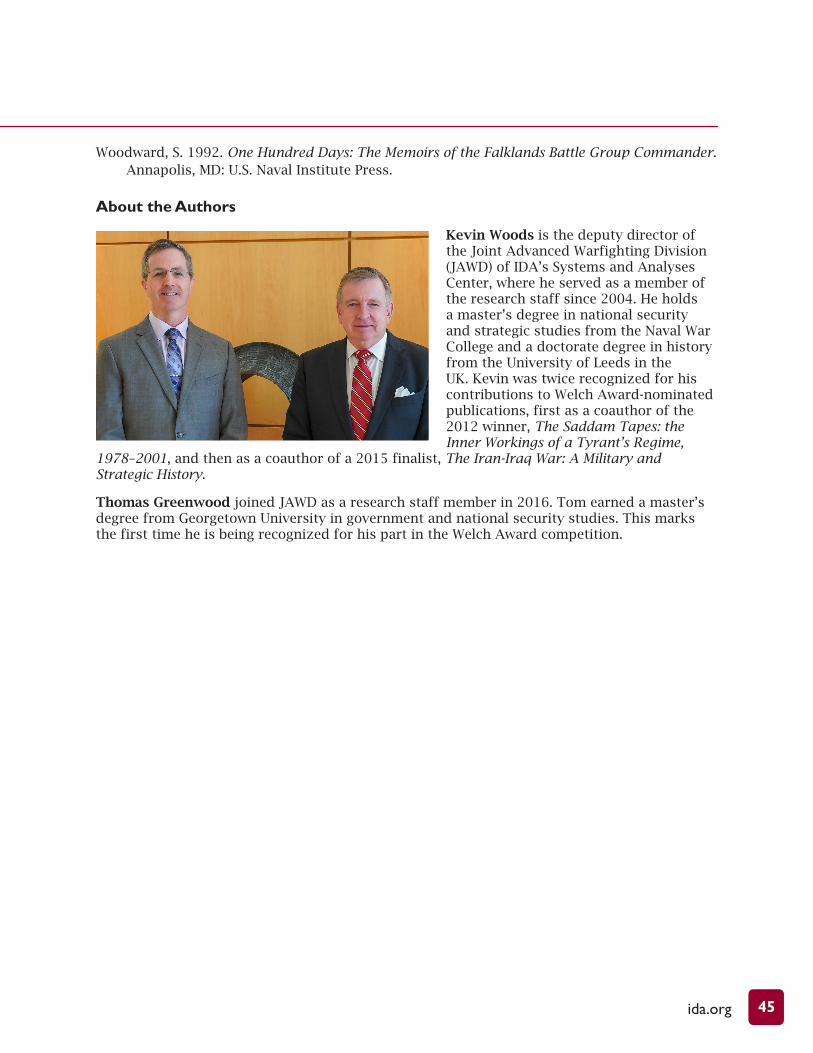
Kevin Woods is the deputy director of the Joint Advanced Warfighting Division (JAWD) of IDA’s Systems and Analyses Center, where he served as a member of the research staff since 2004. He holds a master’s degree in national security and strategic studies from the Naval War College and a doctorate degree in history from the University of Leeds in the UK. Kevin was twice recognized for his contributions to Welch Award-nominated publications, first as a coauthor of the 2012 winner, The Saddam Tapes: the Inner Workings of a Tyrant’s Regime,

1978–2001, and then as a coauthor of a 2015 finalist, The Iran-Iraq War: A Military and Strategic History.

Thomas Greenwood joined JAWD as a research staff member in 2016. Tom earned a master’s degree from Georgetown University in government and national security studies. This marks the first time he is being recognized for his part in the Welch Award competition.

46 RESEARCH NOTES

ida.org 47

Scoping a Test That Has the Wrong Objective1 Thomas H. Johnson, Rebecca M. Medlin, Laura J. Freeman, and James R. Simpson

The Department of Defense test and evaluation community uses power as a key metric for sizing test designs. Power depends on many elements of the design, including the selection of response variables, factors and levels, model formulation, and sample size. The experimental objectives are expressed as hypothesis tests, and power reflects the risk associated with correctly assessing those objectives. Statistical literature refers to a different, yet equally important, type of error that is committed by giving the right answer to the wrong question. If a test design is adequately scoped to address an irrelevant objective, one could say that a Type III error occurs. We focus on a specific Type III error that test planners might commit to reduce test size and resources.

Introduction

Design of experiments is becoming more widely used when testing military systems to aid in planning, executing, and analyzing a test. In the planning phase, critical questions about the system under test are identified and the experimental objectives are set. These questions and objectives guide the development of the response variables, factors, and levels (Freeman et al. 2013).

Equally important in the planning phase is the evaluation of the experimental design. An assortment of measures is available to assess the adequacy of a design prior to data collection. Hahn et al. (1976) call these measures of precision, which include the standard error of predicted mean responses, standard error of coefficients, correlations metrics, and optimality criteria values. Measures of precision are affected by many aspects of the plan, including choice of factors and levels, assumed model form, combination of factor settings from run to run, and total number of runs in the experiment.

Power is an additional and widely used measure of precision, especially in the Department of Defense test and evaluation community. When the objective of an experiment—perhaps determining whether a new weapon system is better than an old system—is expressed as a hypothesis test, power informs risk associated with correctly assessing that objective. Because power increases with sample size, it is a useful metric for determining test length and test resourcing.

An adequate experiment requires sufficient power, but more importantly, it requires the hypothesis tests to reflect accurately the test objectives. If an experiment provides adequate power, but addresses the wrong objective, we might say an error is committed. Kimball (1957) refers to this Type III error as an error of the third kind, describing it as “the error committed by giving the right answer to the wrong question.”

1 Based on “On Scoping a Test That Addresses the Wrong Objective,” Quality Engineering 31, no. 2 (November 2018): 230–239, https://doi.org/10.1080/08982112.2018.1479035.

Despite the perceived in-crease in power and decrease in test resources that comes from reparam-eterization, we conclude that it is not a prudent way to gain test efficiency.

https://doi.org/10.1080/08982112.2018.1479035

48 RESEARCH NOTES

Problem Statement

We focus on a Type III error that test planners might commit in an attempt to reduce test size and test resources. We provide an example that shows how reparameterization of the factor space (i.e., redefining it) from fewer factors with more levels per factor to more factors with fewer levels per factor fundamentally changes the hypothesis tests, which may no longer be aligned with the original objectives of the experiment.

Consider an experiment that plans to characterize a military vehicle’s vulnerability against a particular type of mine. The test program has a limited number of vehicles and mines at their disposal to run a series of destructive tests to characterize the vehicle’s vulnerability.

The measured response variable is the static deformation of the vehicle’s underbody armor plate after interaction with the blast wave and ejecta from the buried charge. In other words, deformation is a direct measurement of the vehicle’s armor shape change with respect to a reference point.

The engineering team believes that the non-uniform placement of structural elements, armor plates, and hardware on the vehicle’s underbody may result in different deformations depending on where the mine is detonated. Thus, the team identifies six underbody detonation locations that may provide unique deformations (Figure 1). The program would like to be able to detect a difference in deformation between any two of the six detonation locations. The necessity for making these comparisons was driven by careful consideration of how mines affect vehicles

Figure 1. Vehicle underbody detonation locations

Intelligence analysts believe that the vehicle is most likely to encounter two variants of the mine type (variant A and B). The program would like to discover if mine variant significantly affects deformation. This discovery could be critical in informing military

ida.org 49

tactics. Additionally, the engineering team would like to determine whether the effect of mine variant on deformation changes as detonation location changes. Thus, the test objectives are as follows: detect a difference in deformation between any two of the six detonation locations, detect a difference in deformation due to mine variant, and detect a change in the effect of mine variant as location changes.

After the test program agrees on these objectives, the test planner sets out to design the experiment. Given the established test objectives, the test planner constructs a twice-replicated factorial experiment using a two-level factor for mine variant and a six-level location factor. Based on the program’s initial allocation of test resources, which accommodate 24 blast events, the test planner finds that the 38% power associated with testing the significance of the location factor and mine variant by location interaction is unsatisfactorily low (as we show in the case study).

Then, the test planner discovers a cost-cutting measure whereby reparameterization of the six-level factor into two factors, a two-level side factor and a three-level position factor (Figure 2), substantially increases power to 89% for the same number of test runs (also shown in the case study).

How could this happen? What information was lost? Is the tester still addressing the original objectives?

Figure 2. Reparameterization of the six-level location factor into a two-level side factor and a three-level position factor

The reparameterization of the factor space changed the hypothesis tests and thus the test objectives. The main effect hypothesis tests in the second proposal no longer correspond to detecting a difference in any two of the six detonation locations on the vehicle, nor does the inclusion of a three-way interaction term in the model correspond to detecting a change in the effect of mine variant as location changes. The tests on the side and position main effects only allow for the detection of a difference between the left and right side, and a difference between any two of the three positions.

50 RESEARCH NOTES

The interaction between these two factors allows for detecting only the effect of one factor (for example, side) differing among the levels of the other factor (for example, position).

In the next section, we show how the test planner’s reparameterization results in a different set of hypothesis tests and different test objectives. (The full version of this article provides additional details on the theory.)

Case Study Example

In this section, we investigate the two test design proposals. In each proposal, the test planner selects static deformation as the response variable of interest, which is normally distributed and measures the deformation of the vehicle’s armor due to the mine blast. Each experimental run consists of a single detonation event, resulting in one measurement of deformation, measured in inches. We refer to the first proposal as the Location Proposal, which differentiates between the six detonation locations using a single factor. We refer to the second proposal as the Side-by-Position Proposal, which changes the six-level location factor into two separate factors. The two proposals include the same mine variant factor. Table 1 lists the factors and levels for each proposal, as well as model parameters for the analysis of variance (ANOVA).

The test planner chooses a main effects plus two-factor interaction model for the Location Proposal and includes an additional three-factor interaction in the Side-by-Position Proposal. The ANOVA model for the Location Proposal is:

μij = μ0 + mi + lj + mlij, i = 1, 2, j = 1 ,..., 6

The ANOVA model for the Side-by-Position Proposal is:

μijk = μ0 + mi + sj + pk + msij + mpik + spjk + mspijk ,

i = 1, 2, j = 1, 2, k = 1, 2, 3.

The effect sizes for the power analysis are first defined in terms of the parameters of the ANOVA model and are then converted into regression model coefficients. In each proposal, the coefficient vector β is of size 12 × 1. Each coefficient vector can be

Table 1. Test design factors, levels, and ANOVA model parameters, shown in parentheses, for the two proposals

Location Proposal Side-by-Position Proposal Factors Mine Location Mine Side Position

Levels A (𝑚𝑚𝑚𝑚1) Left/Back (𝑙𝑙𝑙𝑙1) A (𝑚𝑚𝑚𝑚1) Left (𝑠𝑠𝑠𝑠1) Back (𝑝𝑝𝑝𝑝1) B (𝑚𝑚𝑚𝑚2) Left/Middle (𝑙𝑙𝑙𝑙2) B (𝑚𝑚𝑚𝑚2) Right (𝑠𝑠𝑠𝑠2) Middle (𝑝𝑝𝑝𝑝2)

Left/Front (𝑙𝑙𝑙𝑙3) Front (𝑝𝑝𝑝𝑝3) Right/Back (𝑙𝑙𝑙𝑙4) Right/Middle (𝑙𝑙𝑙𝑙5) Right/Front (𝑙𝑙𝑙𝑙6)

ida.org 51

partitioned by model effects comprising main effects and two-way interactions. The coefficient vector for the Location Proposal is:

The coefficient vector for the Side-by-Position Proposal is:

The design size for each proposal is the same, which is a duplicated full factorial experiment resulting in 24 runs. Let A

l and A

sp denote the single replicate full factorial

model matrix for the Location Proposal and Side-by-Position Proposal, respectively, each of size 12 × 12. The model matrices are where the single replicate full factorial model matrices are constructed according to the following equations:

After defining the models, the test planner is ready to calculate the power associated with assessing the test objectives. Recall, the test objectives are to detect a difference in deformation between any two of the six detonation locations, detect a difference in deformation due to mine variant, and detect a change in the effect of mine variant as location changes. Following typical procedures using statistical software, the test planner assumes that calculating power for main effects and interactions in each proposal addresses the test objectives.

The test planner constructs the hypothesis tests using the equation of the general linear hypothesis test:

where β is the (k+1)×1 vector of coefficients, and k is the number of coefficients in the model excluding the intercept. The t vector specifies the hypothesized constant value of the effect tested and has size q × 1. In practice, t is almost always set to 0. The C matrix isolates the coefficients or combination of coefficients tested and has size q × (k + 1), where q ≤ k + 1. In other words, q is the number of simultaneous hypotheses being tested. The power of the hypothesis test is equal to

where is the F central quantile function that provides the critical F value evaluated at the (1 - α)th quantile, and is the non-central F distribution function evaluated at the critical F value.

5

vector 𝜷𝜷 is of size 12 × 1. Each coefficient vector can be partitioned by model effects comprising main effects and two-way interactions. The coefficient vector for the Location Proposal is:

𝜷𝜷 = [𝛽𝛽0 𝛽𝛽𝑚𝑚 𝜷𝜷𝑙𝑙𝑇𝑇 𝜷𝜷𝑚𝑚𝑙𝑙

𝑇𝑇 ]𝑇𝑇.


𝜷𝜷 = [𝛽𝛽0 𝛽𝛽𝑚𝑚 𝛽𝛽𝑠𝑠 𝜷𝜷𝑝𝑝𝑇𝑇 𝛽𝛽𝑚𝑚𝑠𝑠 𝜷𝜷𝑚𝑚𝑝𝑝

𝑇𝑇 𝜷𝜷𝑠𝑠𝑝𝑝𝑇𝑇 𝜷𝜷𝑚𝑚𝑠𝑠𝑝𝑝

𝑇𝑇 ]𝑇𝑇.

The design size for each proposal is the same, which is a duplicated full factorial experiment resulting in 24 runs. Let 𝑨𝑨𝑙𝑙 and 𝑨𝑨𝑠𝑠𝑝𝑝 denote the single replicate full factorial model matrix for the Location Proposal and Side-by-Position Proposal, respectively, each of size 12 × 12. The model matrices are 𝑿𝑿𝑙𝑙 =[𝑨𝑨𝑙𝑙

𝑇𝑇|𝑨𝑨𝑙𝑙𝑇𝑇] and 𝑿𝑿𝑠𝑠𝑝𝑝 = [𝑨𝑨𝑠𝑠𝑝𝑝

𝑇𝑇 |𝑨𝑨𝑠𝑠𝑝𝑝𝑇𝑇 ], where the single replicate full factorial model matrices are constructed

according to the following equations:

𝑨𝑨𝑙𝑙 = (𝑱𝑱2 ⊗ 𝑱𝑱6|𝚫𝚫2𝑇𝑇 ⊗ 𝑱𝑱6|𝑱𝑱2 ⊗ 𝚫𝚫6

𝑇𝑇|𝚫𝚫2𝑇𝑇 ⊗ 𝚫𝚫6

𝑇𝑇)

𝑨𝑨𝑠𝑠𝑝𝑝 = (𝑱𝑱2 ⊗ 𝑱𝑱2 ⊗ 𝑱𝑱3|𝚫𝚫2𝑇𝑇 ⊗ 𝑱𝑱2 ⊗ 𝑱𝑱3| 𝑱𝑱2 ⊗ 𝚫𝚫2

𝑇𝑇 ⊗ 𝑱𝑱3|𝑱𝑱2 ⊗ 𝑱𝑱2 ⊗ 𝚫𝚫3𝑇𝑇|𝚫𝚫2

𝑇𝑇 ⊗ 𝚫𝚫2𝑇𝑇 ⊗ 𝑱𝑱3|𝚫𝚫2

𝑇𝑇 ⊗ 𝑱𝑱2 ⊗ 𝚫𝚫3𝑇𝑇|𝑱𝑱2

⊗ 𝚫𝚫2𝑇𝑇 ⊗ 𝚫𝚫3


𝑇𝑇 ⊗ 𝚫𝚫3𝑇𝑇)



𝐻𝐻0: 𝑪𝑪𝜷𝜷 = 𝒕𝒕 , 𝐻𝐻1: 𝑪𝑪𝜷𝜷 ≠ 𝒕𝒕,

where 𝜷𝜷 is the (𝑘𝑘 + 1) × 1 vector of coefficients, and 𝑘𝑘 is the number of coefficients in the model excluding the intercept. The 𝒕𝒕 vector specifies the hypothesized constant value of the effect tested and has size 𝑞𝑞 × 1. In practice, 𝒕𝒕 is almost always set to 𝟎𝟎. The 𝑪𝑪 matrix isolates the coefficients or combination of coefficients tested and has size 𝑞𝑞 × (𝑘𝑘 + 1), where 𝑞𝑞 ≤ 𝑘𝑘 + 1. In other words, 𝑞𝑞 is the number of simultaneous hypotheses being tested. The power of the hypothesis test is equal to

𝑃𝑃(𝐹𝐹 ≥ �̂�𝐹𝛼𝛼) = 1 − �̃�𝐹(�̂�𝐹𝛼𝛼,𝑞𝑞,𝑛𝑛−𝑘𝑘−1, 𝑞𝑞, 𝑛𝑛 − 𝑘𝑘 − 1, 𝜆𝜆),

where �̂�𝐹 is the 𝐹𝐹 central quantile function that provides the critical 𝐹𝐹 value evaluated at the (1 − 𝛼𝛼)th quantile, and �̃�𝐹 is the non-central 𝐹𝐹 distribution function evaluated at the critical 𝐹𝐹 value.

Table 2 shows the 𝑪𝑪 matrix associated with each hypothesis test on the main effects and interactions for the two proposals. The hypothesis tests in this table assume that 𝒕𝒕 is equal to 𝟎𝟎.

5



𝑇𝑇 ]𝑇𝑇.




𝑇𝑇 ]𝑇𝑇.







𝑇𝑇)















5



𝑇𝑇 ]𝑇𝑇.




𝑇𝑇 ]𝑇𝑇.







𝑇𝑇)















5



𝑇𝑇 ]𝑇𝑇.




𝑇𝑇 ]𝑇𝑇.







𝑇𝑇)















5



𝑇𝑇 ]𝑇𝑇.




𝑇𝑇 ]𝑇𝑇.







𝑇𝑇)















5



𝑇𝑇 ]𝑇𝑇.




𝑇𝑇 ]𝑇𝑇.







𝑇𝑇)















5



𝑇𝑇 ]𝑇𝑇.




𝑇𝑇 ]𝑇𝑇.







𝑇𝑇)















5



𝑇𝑇 ]𝑇𝑇.




𝑇𝑇 ]𝑇𝑇.







𝑇𝑇)















5



𝑇𝑇 ]𝑇𝑇.




𝑇𝑇 ]𝑇𝑇.







𝑇𝑇)















52 RESEARCH NOTES

Table 2 shows the C matrix associated with each hypothesis test on the main effects and interactions for the two proposals. The hypothesis tests in this table assume that t is equal to 0.

Next, the test planner defines the effect sizes. An effect size is defined for each hypothesis test and represents the value of the coefficients tested assuming H0 is false and H1 is true. Using the unified approach (see the original article for details), the test planner first defines the effect size in terms of parameters of the ANOVA model and then converts those parameters into coefficients for the regression model.

The test planner selects an effect size of 1 inch. In the Location Proposal, letting m, l, and ml be the vectors of the ANOVA model parameters for mi, lj, and mlij. The effect size definition implies that the range of m, l, or ml is equal to 1 inch. Using a similar approach in the Side-by-Position Proposal, the effect size implies the range of m,s,p,ms,mp,sp,or msp is equal to 1 inch.

Part two of the unified approach requires a search among the candidate set of effect sizes for the particular effect size that yields minimum power. The candidate search is unnecessary in this case study because the test designs are completely balanced. For balanced designs, power for each effect size within a candidate set is identical. It is only with unbalanced designs that the candidate search is necessary to provide a unique estimate of power.

The test planner defines the individual ANOVA model parameter vectors to satisfy part one of the unified approach. To illustrate for l in the first proposal, the test planner arbitrarily chooses the configuration shown below. (Another configuration could have been selected because each gives the same power because the design is balanced. See Table 2 in the original article for all design configurations.)

The equation that converts the ANOVA model parameter to the regression model coefficients is

Table 2. Hypothesis Test for Each Proposal

Location Proposal Size-by-Position Proposal Hypothesis 𝐶𝐶𝐶𝐶 Hypothesis 𝐶𝐶𝐶𝐶 𝐻𝐻𝐻𝐻0:𝛽𝛽𝛽𝛽𝑚𝑚𝑚𝑚 = 0 �0 1 𝟎𝟎𝟎𝟎

1×10� 𝐻𝐻𝐻𝐻0:𝛽𝛽𝛽𝛽𝑚𝑚𝑚𝑚 = 0 �0 1 𝟎𝟎𝟎𝟎1×10�

𝐻𝐻𝐻𝐻0:𝜷𝜷𝜷𝜷𝑙𝑙𝑙𝑙 = 𝟎𝟎𝟎𝟎 � 𝟎𝟎𝟎𝟎5×2𝑰𝑰𝑰𝑰5 𝟎𝟎𝟎𝟎

5×5� 𝐻𝐻𝐻𝐻0:𝛽𝛽𝛽𝛽𝑠𝑠𝑠𝑠 = 0 � 𝟎𝟎𝟎𝟎1×21 𝟎𝟎𝟎𝟎

1×9� 𝐻𝐻𝐻𝐻0:𝜷𝜷𝜷𝜷𝑚𝑚𝑚𝑚𝑙𝑙𝑙𝑙 = 𝟎𝟎𝟎𝟎 � 𝟎𝟎𝟎𝟎5×7

𝑰𝑰𝑰𝑰5� 𝐻𝐻𝐻𝐻0:𝜷𝜷𝜷𝜷𝑝𝑝𝑝𝑝 = 𝟎𝟎𝟎𝟎 � 𝟎𝟎𝟎𝟎2×3𝑰𝑰𝑰𝑰2 𝟎𝟎𝟎𝟎

2×7� 𝐻𝐻𝐻𝐻0:𝛽𝛽𝛽𝛽𝑚𝑚𝑚𝑚𝑠𝑠𝑠𝑠 = 0 � 𝟎𝟎𝟎𝟎1×5

1 𝟎𝟎𝟎𝟎1×6�

𝐻𝐻𝐻𝐻0:𝜷𝜷𝜷𝜷𝑚𝑚𝑚𝑚𝑝𝑝𝑝𝑝 = 𝟎𝟎𝟎𝟎 � 𝟎𝟎𝟎𝟎2×6𝑰𝑰𝑰𝑰2 𝟎𝟎𝟎𝟎

2×4�

6


Location Proposal Size-by-Position Proposal Hypothesis 𝐶𝐶 Hypothesis 𝐶𝐶 𝐻𝐻0: 𝛽𝛽𝑚𝑚 = 0 [0 1 𝟎𝟎

1×10] 𝐻𝐻0: 𝛽𝛽𝑚𝑚 = 0 [0 1 𝟎𝟎1×10]

𝐻𝐻0: 𝜷𝜷𝑙𝑙 = 𝟎𝟎 [ 𝟎𝟎5×2

𝑰𝑰5 𝟎𝟎5×5] 𝐻𝐻0: 𝛽𝛽𝑠𝑠 = 0 [ 𝟎𝟎

1×21 𝟎𝟎

1×9] 𝐻𝐻0: 𝜷𝜷𝑚𝑚𝑙𝑙 = 𝟎𝟎 [ 𝟎𝟎

5×7𝑰𝑰5] 𝐻𝐻0: 𝜷𝜷𝑝𝑝 = 𝟎𝟎 [ 𝟎𝟎

2×3𝑰𝑰2 𝟎𝟎

2×7] 𝐻𝐻0: 𝛽𝛽𝑚𝑚𝑠𝑠 = 0 [ 𝟎𝟎

1×51 𝟎𝟎

1×6] 𝐻𝐻0: 𝜷𝜷𝑚𝑚𝑝𝑝 = 𝟎𝟎 [ 𝟎𝟎

2×6𝑰𝑰2 𝟎𝟎

2×4]

Next, the test planner defines the effect sizes. An effect size is defined for each hypothesis test and represents the value of the coefficients tested assuming 𝐻𝐻0 is false and 𝐻𝐻1 is true. Using the unified approach (see the original article for details), the test planner first defines the effect size in terms of parameters of the ANOVA model and then converts those parameters into coefficients for the regression model.

The test planner selects an effect size of 1 inch. In the Location Proposal, letting 𝒎𝒎, 𝒍𝒍, and 𝒎𝒎𝒍𝒍 be the vectors of the ANOVA model parameters for 𝑚𝑚𝑖𝑖, 𝑙𝑙𝑗𝑗, and 𝑚𝑚𝑙𝑙𝑖𝑖𝑗𝑗. The effect size definition implies that the range of 𝒎𝒎, 𝒍𝒍, or 𝒎𝒎𝒍𝒍 is equal to 1 inch. Using a similar approach in the Side-by-Position Proposal, the effect size implies the range of 𝒎𝒎, 𝒔𝒔, 𝒑𝒑, 𝒎𝒎𝒔𝒔, 𝒎𝒎𝒑𝒑, 𝒔𝒔𝒑𝒑, 𝒐𝒐𝒐𝒐 𝒎𝒎𝒔𝒔𝒑𝒑 is equal to 1 inch.


The test planner defines the individual ANOVA model parameter vectors to satisfy part one of the unified approach. To illustrate for 𝑙𝑙 in the first proposal, the test planner arbitrarily chooses the configuration shown below. (Another configuration could have been selected because each gives the same power because the design is balanced. See Table 2 in the original article for all design configurations.)

𝒍𝒍 = [1/2 0 0 0 0 − 1/2]𝑇𝑇


𝜷𝜷𝑙𝑙 = (𝚫𝚫6𝑇𝑇)−1𝒍𝒍 = [1/2 0 0 0 0 ]𝑇𝑇.

The conversion for two- and three-factor interactions follows a similar process. Take, for example, the 𝒎𝒎𝒍𝒍 interaction in the first proposal. The test planner arbitrarily chooses the configuration, and the ANOVA model parameter vector is

𝒎𝒎𝒍𝒍 = [1/2 0 − 1/2 0 0 0 − 1/2 0 1/2 0 0 0]𝑇𝑇.

The equation that converts the ANOVA model parameter to regression model coefficients is

6



1×10] 𝐻𝐻0: 𝛽𝛽𝑚𝑚 = 0 [0 1 𝟎𝟎1×10]

𝐻𝐻0: 𝜷𝜷𝑙𝑙 = 𝟎𝟎 [ 𝟎𝟎5×2

𝑰𝑰5 𝟎𝟎5×5] 𝐻𝐻0: 𝛽𝛽𝑠𝑠 = 0 [ 𝟎𝟎

1×21 𝟎𝟎

1×9] 𝐻𝐻0: 𝜷𝜷𝑚𝑚𝑙𝑙 = 𝟎𝟎 [ 𝟎𝟎

5×7𝑰𝑰5] 𝐻𝐻0: 𝜷𝜷𝑝𝑝 = 𝟎𝟎 [ 𝟎𝟎

2×3𝑰𝑰2 𝟎𝟎

2×7] 𝐻𝐻0: 𝛽𝛽𝑚𝑚𝑠𝑠 = 0 [ 𝟎𝟎

1×51 𝟎𝟎

1×6] 𝐻𝐻0: 𝜷𝜷𝑚𝑚𝑝𝑝 = 𝟎𝟎 [ 𝟎𝟎

2×6𝑰𝑰2 𝟎𝟎

2×4]





𝒍𝒍 = [1/2 0 0 0 0 − 1/2]𝑇𝑇


𝜷𝜷𝑙𝑙 = (𝚫𝚫6𝑇𝑇)−1𝒍𝒍 = [1/2 0 0 0 0 ]𝑇𝑇.


𝒎𝒎𝒍𝒍 = [1/2 0 − 1/2 0 0 0 − 1/2 0 1/2 0 0 0]𝑇𝑇.


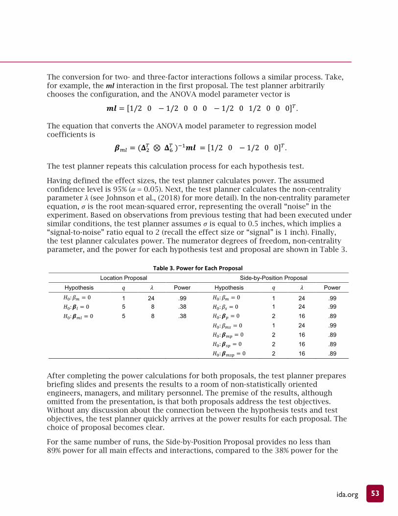
ida.org 53

The conversion for two- and three-factor interactions follows a similar process. Take, for example, the ml interaction in the first proposal. The test planner arbitrarily chooses the configuration, and the ANOVA model parameter vector is


The test planner repeats this calculation process for each hypothesis test.

Having defined the effect sizes, the test planner calculates power. The assumed confidence level is 95% (α = 0.05). Next, the test planner calculates the non-centrality parameter λ (see Johnson et al., (2018) for more detail). In the non-centrality parameter equation, σ is the root mean-squared error, representing the overall “noise” in the experiment. Based on observations from previous testing that had been executed under similar conditions, the test planner assumes σ is equal to 0.5 inches, which implies a “signal-to-noise” ratio equal to 2 (recall the effect size or “signal” is 1 inch). Finally, the test planner calculates power. The numerator degrees of freedom, non-centrality parameter, and the power for each hypothesis test and proposal are shown in Table 3.

After completing the power calculations for both proposals, the test planner prepares briefing slides and presents the results to a room of non-statistically oriented engineers, managers, and military personnel. The premise of the results, although omitted from the presentation, is that both proposals address the test objectives. Without any discussion about the connection between the hypothesis tests and test objectives, the test planner quickly arrives at the power results for each proposal. The choice of proposal becomes clear.

For the same number of runs, the Side-by-Position Proposal provides no less than 89% power for all main effects and interactions, compared to the 38% power for the

6



1×10] 𝐻𝐻0: 𝛽𝛽𝑚𝑚 = 0 [0 1 𝟎𝟎1×10]

𝐻𝐻0: 𝜷𝜷𝑙𝑙 = 𝟎𝟎 [ 𝟎𝟎5×2

𝑰𝑰5 𝟎𝟎5×5] 𝐻𝐻0: 𝛽𝛽𝑠𝑠 = 0 [ 𝟎𝟎

1×21 𝟎𝟎

1×9] 𝐻𝐻0: 𝜷𝜷𝑚𝑚𝑙𝑙 = 𝟎𝟎 [ 𝟎𝟎

5×7𝑰𝑰5] 𝐻𝐻0: 𝜷𝜷𝑝𝑝 = 𝟎𝟎 [ 𝟎𝟎

2×3𝑰𝑰2 𝟎𝟎

2×7] 𝐻𝐻0: 𝛽𝛽𝑚𝑚𝑠𝑠 = 0 [ 𝟎𝟎

1×51 𝟎𝟎

1×6] 𝐻𝐻0: 𝜷𝜷𝑚𝑚𝑝𝑝 = 𝟎𝟎 [ 𝟎𝟎

2×6𝑰𝑰2 𝟎𝟎

2×4]





𝒍𝒍 = [1/2 0 0 0 0 − 1/2]𝑇𝑇


𝜷𝜷𝑙𝑙 = (𝚫𝚫6𝑇𝑇)−1𝒍𝒍 = [1/2 0 0 0 0 ]𝑇𝑇.


𝒎𝒎𝒍𝒍 = [1/2 0 − 1/2 0 0 0 − 1/2 0 1/2 0 0 0]𝑇𝑇.


7

𝜷𝜷𝑚𝑚𝑚𝑚 = (𝚫𝚫2𝑇𝑇 ⊗ 𝚫𝚫6

𝑇𝑇 )−1𝒎𝒎𝒎𝒎 = [1/2 0 − 1/2 0 0]𝑇𝑇.

The test planner repeats this calculation process for each hypothesis test.

Having defined the effect sizes, the test planner calculates power. The assumed confidence level is 95% (𝛼𝛼 = 0.05). Next, the test planner calculates the non-centrality parameter 𝜆𝜆 (see Johnson et al., (2018) for more detail). In the non-centrality parameter equation, 𝜎𝜎 is the root mean-squared error, representing the overall “noise” in the experiment. Based on observations from previous testing that had been executed under similar conditions, the test planner assumes 𝜎𝜎 is equal to 0.5 inches, which implies a “signal-to-noise” ratio equal to 2 (recall the effect size or “signal” is 1 inch). Finally, the test planner calculates power. The numerator degrees of freedom, non-centrality parameter, and the power for each hypothesis test and proposal are shown in Table 3.

Table 3. Power for Each Proposal

Location Proposal Side-by-Position Proposal Hypothesis 𝑞𝑞 𝜆𝜆 Power Hypothesis 𝑞𝑞 𝜆𝜆 Power 𝐻𝐻0: 𝛽𝛽𝑚𝑚 = 0 1 24 .99 𝐻𝐻0: 𝛽𝛽𝑚𝑚 = 0 1 24 .99 𝐻𝐻0: 𝜷𝜷𝑚𝑚 = 0 5 8 .38 𝐻𝐻0: 𝛽𝛽𝑠𝑠 = 0 1 24 .99 𝐻𝐻0: 𝜷𝜷𝑚𝑚𝑚𝑚 = 0 5 8 .38 𝐻𝐻0: 𝜷𝜷𝑝𝑝 = 0 2 16 .89

𝐻𝐻0: 𝛽𝛽𝑚𝑚𝑠𝑠 = 0 1 24 .99 𝐻𝐻0: 𝜷𝜷𝑚𝑚𝑝𝑝 = 0 2 16 .89 𝐻𝐻0: 𝜷𝜷𝑠𝑠𝑝𝑝 = 0 2 16 .89 𝐻𝐻0: 𝜷𝜷𝑚𝑚𝑠𝑠𝑝𝑝 = 0 2 16 .89

After completing the power calculations for both proposals, the test planner prepares briefing slides and presents the results to a room of non-statistically oriented engineers, managers, and military personnel. The premise of the results, although omitted from the presentation, is that both proposals address the test objectives. Without any discussion about the connection between the hypothesis tests and test objectives, the test planner quickly arrives at the power results for each proposal. The choice of proposal becomes clear.

For the same number of runs, the Side-by-Position Proposal provides no less than 89% power for all main effects and interactions, compared to the 38% power for the Location Proposal. Impressed by the savings in test resources, the test program agrees to the Side-by-Position Proposal and commits a Type III error.

CCoonncclluussiioonn

The test planner mistakenly believed that the main effects and interaction hypothesis tests in the Side-by-Position Proposal addressed the test objectives. In truth, the tests on the main effects allow for the detection of a difference between the left and right sides, and a difference between any two of the

Table 3. Power for Each Proposal Location Proposal Side-by-Position Proposal

Hypothesis 𝑞𝑞𝑞𝑞 𝜆𝜆𝜆𝜆 Power Hypothesis 𝑞𝑞𝑞𝑞 𝜆𝜆𝜆𝜆 Power 𝐻𝐻𝐻𝐻0:𝛽𝛽𝛽𝛽𝑚𝑚𝑚𝑚 = 0 1 24 .99 𝐻𝐻𝐻𝐻0:𝛽𝛽𝛽𝛽𝑚𝑚𝑚𝑚 = 0 1 24 .99 𝐻𝐻𝐻𝐻0:𝜷𝜷𝜷𝜷𝑙𝑙𝑙𝑙 = 0 5 8 .38 𝐻𝐻𝐻𝐻0:𝛽𝛽𝛽𝛽𝑠𝑠𝑠𝑠 = 0 1 24 .99 𝐻𝐻𝐻𝐻0:𝜷𝜷𝜷𝜷𝑚𝑚𝑚𝑚𝑙𝑙𝑙𝑙 = 0 5 8 .38 𝐻𝐻𝐻𝐻0:𝜷𝜷𝜷𝜷𝑝𝑝𝑝𝑝 = 0 2 16 .89

𝐻𝐻𝐻𝐻0:𝛽𝛽𝛽𝛽𝑚𝑚𝑚𝑚𝑠𝑠𝑠𝑠 = 0 1 24 .99 𝐻𝐻𝐻𝐻0:𝜷𝜷𝜷𝜷𝑚𝑚𝑚𝑚𝑝𝑝𝑝𝑝 = 0 2 16 .89 𝐻𝐻𝐻𝐻0:𝜷𝜷𝜷𝜷𝑠𝑠𝑠𝑠𝑝𝑝𝑝𝑝 = 0 2 16 .89 𝐻𝐻𝐻𝐻0:𝜷𝜷𝜷𝜷𝑚𝑚𝑚𝑚𝑠𝑠𝑠𝑠𝑝𝑝𝑝𝑝 = 0 2 16 .89

54 RESEARCH NOTES

Location Proposal. Impressed by the savings in test resources, the test program agrees to the Side-by-Position Proposal and commits a Type III error.

Conclusion

The test planner mistakenly believed that the main effects and interaction hypothesis tests in the Side-by-Position Proposal addressed the test objectives. In truth, the tests on the main effects allow for the detection of a difference between the left and right sides, and a difference between any two of the three positions, respectively. Neither of these hypothesis tests, nor the interaction test, allows for the detection of a difference between any two of the six locations on the vehicle. The perceived high power associated with this proposal led the team to believe the test was adequately resourced. Despite the perceived increase in power and decrease in test resources that comes from reparameterization, we conclude that it is not a prudent way to gain test efficiency.

In this particular example, the high power was not used to argue for a smaller test design, but this could and does happen in practice. The proper decision would have been to select the Location Proposal, and recognize that the only solution to adequately assessing the test objectives is to add more experimental runs.

The case study highlights potential negative consequences of redefining a factor space, but the approach should not be completely discredited. If the test planner and the test program had renegotiated the objectives, such that the objectives aligned with the hypothesis tests in the Side-by-Position Proposal, reparameterization could have been a shrewd cost-saving strategy. It is the lack of careful planning that leads to a Type III error.

The unified effect size approach, coupled with the ability to convert effect sizes between the ANOVA and regression model formulations, facilitated the diagnosis of the Type III error. These tools were useful for comparing reparameterizations of a factor space for a fixed experimental design, but they can also be useful for comparing competing designs that have different sample sizes or different degrees of imbalance. The consistent estimate of power from the unified approach enables such comparisons.

ReferencesFreeman, L. J., A. G. Ryan, J. L. K. Kensler, R. M. Dickinson, and G. G. Vining. 2013. “A Tutorial

on the Planning of Experiments.” Quality Engineering 25, no. 4: 315–332. https://doi.org/10.1080/08982112.2013.817013.

Hahn, G. J., W. Q. Meeker Jr, and P. I. Feder.1976. “The Evaluation and Comparison of Experimental Designs for Fitting Regression Relationships.” Journal of Quality Technology 8, no. 3: 140–157. https://doi.org/10.1080/00224065.1976.11980735.

Kimball, A. W. 1957. “Errors of the Third Kind in Statistical Consulting.” Journal of the American Statistical Association 52, no. 278: 133–142. https://doi.org/10.1080/01621459.1957.10501374.

https://doi.org/10.1080/08982112.2013.817013

https://doi.org/10.1080/00224065.1976.11980735

https://doi.org/10.1080/01621459.1957.10501374

ida.org 55

About the Authors

Thomas Johnson is a member of the research staff of the Operational Evaluation Division (OED) of IDA’s Systems and Analyses Center. Tom joined IDA in 2011. Both his master’s degree and his doctorate degree are in aerospace engineering from Old Dominion University. Tom was twice recognized as a coauthor of finalist Welsh Award publications, for “Power Approximations for Generalized Linear Models Using the Signal-to-Noise Transformation Method” in 2018 and for “A Comparison of Ballistic Resistance Testing Techniques in the Department of Defense” in 2015.

Rebecca Medlin joined IDA in 2015 as a member of OED’s research staff. She earned both her master’s and doctorate degrees in statistics from Virginia Polytechnic Institute and State University. Rebecca is being recognized for the first time this year as a finalist coauthor in the Welch Award competition.

Laura Freeman was first a research staff member and then an assistant director in OED during her tenure at IDA, which ended in 2019. She earned her master’s and doctoral degrees in statistics, both from Virginia Polytechnic Institute and State University. Laura was a coauthor of two other Welch Award finalist publications: “Power Approximations for Generalized Linear Models Using the Signal-to-Noise Transformation Method” in 2018 and “A Comparison of Ballistic Resistance Testing Techniques in the Department of Defense” in 2015.

James Simpson, an OED consultant, holds a doctorate in industrial engineering from Arizona State University. He was recognized as a coauthor of the 2018 Welch Award finalist publication “Power Approximations for Generalized Linear Models Using the Signal-to-Noise Transformation Method.”

research notes - ida.org

Documents