research open access spatial filter decomposition for ... · spatial filter decomposition for...
TRANSCRIPT

Maoudj et al. EURASIP Journal on Advances in Signal Processing 2014, 2014:127http://asp.eurasipjournals.com/content/2014/1/127
RESEARCH Open Access
Spatial filter decomposition for interferencemitigationRabah Maoudj1*, Michel Terre1, Luc Fety1, Christophe Alexandre1 and Philippe Mege2
Abstract
This paper presents a two-part decomposition of a spatial filter having to optimize the reception of a useful signalin the presence of an important co-channel interference level. The decomposition highlights the role of two partsof the filter, one devoted to the maximization of the signal to noise ratio and the other devoted to the interferencecancellation. The two-part decomposition is used in the estimation process of the optimal reception filter. Wepropose then an estimation algorithm that follows this decomposition, and the global spatial filter is finally obtainedthrough an optimal-weighted combination of two filters. It is shown that this two-component-based decompositionalgorithm overcomes other previously published solutions involving eigenvalue decompositions.
Keywords: SIMO receiver; Optimum combining; Maximum ratio combining; Antenna array
1 IntroductionIncreasing capacity demand for wireless communicationnetworks should lead to a high co-channel interferencelevel in the future. This interference problem is not newand has been addressed, for a long time, in wirelessnetworks. The first solutions, coming from 2G networks,were based on frequency reuse patterns while, a few yearslater, scrambling codes were used, for the same purpose,in 3G networks. Nowadays, diversity techniques are moreand more considered as one of the best answer for thisinterference problem, especially in 4G networks. The workpresented in this paper was initially based on privatemobile radio (PMR) characteristics linked to the TETRAenhanced data service (TEDS) standard, but it is suitablealso in the context of 4G transmissions which are based onthe Long-Term Evolution (LTE) standard. The presentedwork addresses essentially the problem of transmission withhigh interference level ratio and fast varying propagationchannels.In such a context, several previous works have treated
and analyzed the best spatial filter to maximize thesignal to interference plus noise ratio (SINR). Theoptimum combining (OC) filter [1-5] can be proposedas an exploitable solution. It was also proven that, inthe absence of interference, this optimum combining
* Correspondence: [email protected]/CEDRIC/Laetitia, Paris, FranceFull list of author information is available at the end of the article
© 2014 Maoudj et al.; licensee Springer. This isAttribution License (http://creativecommons.orin any medium, provided the original work is p
filter converges to the well-known maximum ratiocombining (MRC) filter [6].The main problem, in the estimation of the optimum
combiner filter, resides in the estimation of the covariancematrix of the interference plus noise in addition to theestimation of the useful user propagation channel. Theminimum mean square error estimation (MMSE) criterioncan be used to estimate the desired user propagation chan-nel, while the covariance matrix can be estimated by thesample matrix inversion (SMI) approach [7-9]. However,this strategy is suboptimal and requires a large signalsample set to get a correct smoothing stage [10,11].Another problem resides in the covariance matrix itselfwhich will be obviously interpolated to the data locationssince it is estimated on the pilot locations [10].In this paper, we will prove that under certain condi-
tions, the OC filter can perfectly be decomposed in twoindependent components. Hence, when the number ofinterferers is smaller than the number of receiving anten-nas, the OC filter can be split in two weighted components,namely MRC filter and interference canceller combiner(ICC). Moreover, for its own scientific interest, it will beproven that this decomposition leads to a new and efficientoptimum filter estimation algorithm.More precisely, we will show that for the MRC part of
the OC filter, the classical MMSE can be proposed in orderto obtain the estimation of the useful user propagationchannel. On the other hand, we will show that the ICC part
an Open Access article distributed under the terms of the Creative Commonsg/licenses/by/4.0), which permits unrestricted use, distribution, and reproductionroperly credited.

Maoudj et al. EURASIP Journal on Advances in Signal Processing 2014, 2014:127 Page 2 of 14http://asp.eurasipjournals.com/content/2014/1/127
can be estimated by modifying the matched desired impulseresponse (MDIR) algorithm [12]. This algorithm requiresa null linear system solving, and a constraint is required toprevent the trivial solution. Following [12], a constraint,so-called maximum SINR constraint (MSINRC), can beintroduced; it will maximize the SINR at the output ofthe filter. The final solution-vector will then be given bythe eigenvector corresponding to the lowest eigenvalueof a Hermitian matrix generated by the algorithm. Dueto the presence of the noise, the estimation still remainssuboptimal and the result is corrupted by the trainingnoise estimation. It was proven in [13] that combining alleigenvectors, weighted by the inverse of their correspond-ing output SINR, could lead to an enhanced algorithm,so-called solution-vectors maximum ratio combining(SoMRC). It was shown that this approach gives betterperformance than the single solution-vector [13,14]. Obvi-ously, such kind of algorithms is based on a complexeigendecomposition. To simplify this step, we proposeto introduce another constraint, leading to a less complexalgorithm where we can avoid the eigendecomposition.We will also show that this new constraint keeps theperformance of the algorithm comparable to that of theSoMRC.The contribution of the presented work in the study of
the optimum combiner filter consists on identifying thecases where it can be decomposed to a MRC plus a ICCindependent filters. Another contribution consists ofthe modified MDIR algorithm and in the introductionof the new constraint that does not degrade performancesof the SoMRC. A 16-bit digital signal processor (DSP)implementation is also presented in order to evaluate therounding errors effect on the performance of the algorithmand to determine the possibility of the algorithm executionunder some real-time constraints.The paper is organized as follows. The system model
is given in Section 2. Section 3 presents the split of theOC into two weighted independent parts, namely MRCand ICC. In Section 4, the estimation algorithm for ICCis detailed. A simplification of this estimation algorithmis introduced in Section 5. Numerical results and per-formance of the algorithms are presented in Section 6. Aperformance degradation study, due to a practical 16-bitfixed point DSP implementation is detailed in Section 7.Conclusion summarizes the present work in Section 8.
1.1 NotationVectors and matrices are boldface small and capital letters;the transpose, complex conjugate transpose, and inverseof matrix A are denoted by AT, AH, and A−1, respectively.The norm of vector a and the diagonal matrix with the
diagonal element extracted from a are denoted respect-ively by ‖a‖ and diag{a}, IN is the N×N identity matrix,and E[.] denotes the statistical expectation.
2 System modelWe consider a SIMO structure having M receiving anten-nas, with one desired signal and U interferers, as presentedin Figure 1. Desired user and interferers are transmittingorthogonal frequency-division multiplexing (OFDM) wave-forms, and for the sake of simplicity, we will consider thatall users are time and frequency synchronized. This remarkis not restrictive, and all results presented are notlinked to this hypothesis that will nevertheless simplifysome notations in the sequel of the paper.The OFDM frame of the desired user is composed of
K subcarriers and Ns OFDM symbols. A Ng length cyclicprefix is inserted. It is assumed that this cyclic prefix issufficient to totally suppress intersymbol interferences.We will focus on one OFDM symbol, and we will avoidindicating the symbol number in the notations. Algo-rithms presented will then be able to cope with a uniqueOFDM symbol and therefore able to deal with veryhigh-speed propagation channels.With this assumption, the received sample, after the
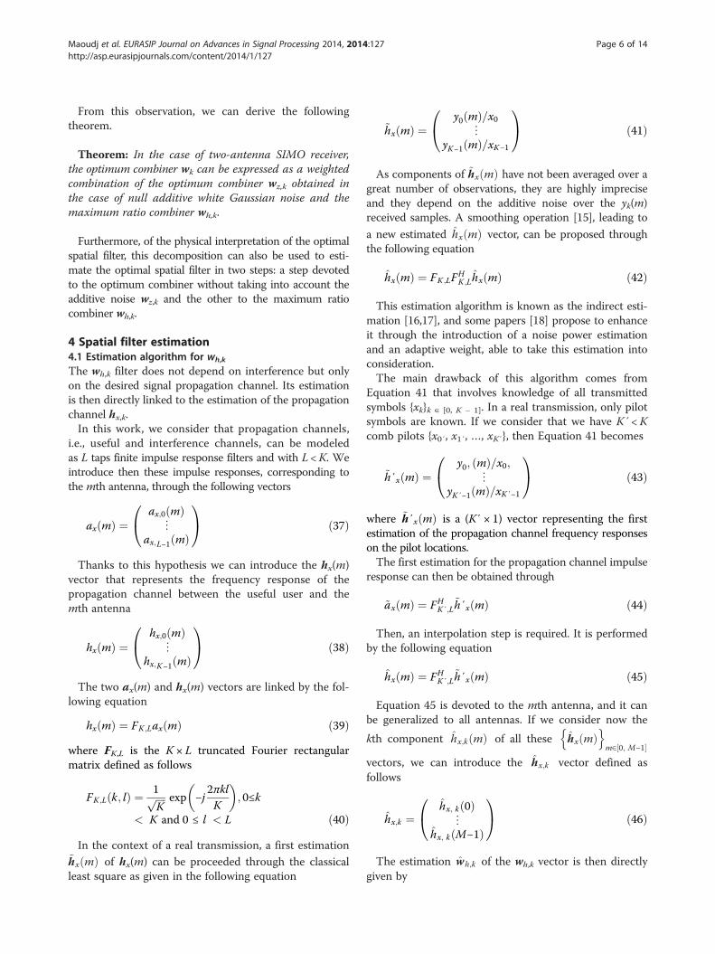
OFDM demodulation, corresponding to the kth subcarrieron the mth antenna, as presented in Figure 2, can bemodeled by Equation 1:
yk mð Þ ¼ hx;k mð Þxk þ nIk mð Þ ð1Þ
nIk mð Þ denotes an additive noise plus interference termand can be developed as follows
nIk mð Þ ¼XU
u¼1hz;k;u mð Þzk;u þ nk mð Þ ð2Þ
Zk,u is the symbol transmitted by the uth interferer.hz,k,u(m) denotes the frequency response of the channel
between the uth interferer and the mth antenna. nk(m)represents a centered additive white Gaussian noise term
with a variance equals to σn2.XU
u¼1hz;k;u mð Þzk;u is then the total contribution of the
U interferers received by the mth antenna on the kthsubcarrier.In this paper, we have to identify a spatial filter wk able to
estimate the QAM symbol xk transmitted by the desireduser. This leads to
xk ¼ wHk yk ð3Þ
In this equation, corresponding to the kth subcarrier,
wk ¼wk 0ð Þ
⋮wk M−1ð Þ
0@
1A denotes, as illustrated in Figure 3,
M weights of the spatial filter and yk ¼yk 0ð Þ⋮
yk M−1ð Þ
0@
1A
stands for the kth post-fast Fourier transform (FFT) outputs
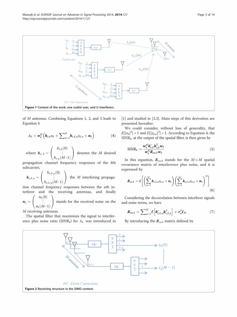
Figure 1 Context of the work, one useful user, and U interferers.
Maoudj et al. EURASIP Journal on Advances in Signal Processing 2014, 2014:127 Page 3 of 14http://asp.eurasipjournals.com/content/2014/1/127
of M antennas. Combining Equations 1, 2, and 3 leads toEquation 4
xk ¼ wHk hx;kxk þ
XU
u¼1hz;k;uzk;u þ nk
� �ð4Þ
where hx; k ¼hx;k 0ð Þ
⋮hx;k M−1ð Þ
0@
1A denotes the M desired
propagation channel frequency responses of the kthsubcarrier,
hx;k ;u ¼hx;k ;u 0ð Þ
⋮hx;k ;u M−1ð Þ
0@
1A the M interfering propaga-
tion channel frequency responses between the uth in-terferer and the receiving antennas, and finally
nk ¼nk 0ð Þ⋮
nk M−1ð Þ
0@
1A stands for the received noise on the
M receiving antennas.The spatial filter that maximizes the signal to interfer-
ence plus noise ratio (SINRk) for xk was introduced in
Figure 2 Receiving structure in the SIMO context.
[1] and studied in [2,3]. Main steps of this derivation arepresented hereafter.We could consider, without loss of generality, that
E[|xk|2] = 1 and E[|zk,u|
2] = 1. According to Equation 4, theSINRk, at the output of the spatial filter, is then given by
SINRk ¼wH
k h�x;kh
Tx;kwk
wHk Rnn;kwk
ð5Þ
In this equation, Rnn,k stands for the M×M spatialcovariance matrix of interference plus noise, and it isexpressed by
Rnn;k ¼ EXUu¼1
hz;k;uzk;u þ nk
! XUu¼1
hz;k;uzk;u þ nk
!H" #
ð6ÞConsidering the decorrelation between interferer signals
and noise terms, we have
Rnn;k ¼XU
u¼1E h�z;k;uh
Tz;k;u
h iþ σ2nIM ð7Þ
By introducing the Rzz,k matrix defined by

Figure 3 Receiver spatial filter for the kth subcarrier.
Maoudj et al. EURASIP Journal on Advances in Signal Processing 2014, 2014:127 Page 4 of 14http://asp.eurasipjournals.com/content/2014/1/127
Rzz;k ¼XU
u¼1E h�z;k;uh
Tz;k;u
h ið8Þ
we can rewrite Rnn,k as a summation of two parts asgiven hereafter
Rnn;k ¼ Rzz;k þ σ2nI ð9Þ
At the output of the combiner, in order to perfectlyequalize the useful channel, we propose to introduce thefollowing constraint
wHk h
�x;k ¼ 1 ð10Þ
Merging Equations 5 and 9, the SINRk becomes
SINRk ¼ 1wH
k Rnn;kwkð11Þ
The optimum spatial filter vector wk that maximizesthe SINRk can then be obtained by minimizing wH
k Rnn;k
wk under the constraint wHk h
�x;k ¼ 1 . Using Lagrange
multiplier, the optimum spatial filter is obtained by solvingthe following equation
wk ¼ argmin L 1SINRk
;wk ; λ
� �ð12Þ
where the Lagrangian is defined such that
L1
SINRk;wk ; λ
� �¼ wH
k Rnn;kwk−λ wHk h
�x;k−1
� �ð13Þ
Under the assumption that detd2L 1
SNIRk;wk ;λ
� �dw2
k
0@
1A > 0 ,
the solution is obtained by nulling the derivative of
L 1SNIRk
;wk ; λ� �
with respect to wk
dL 1SINRk
;wk ; λ� �
dwk¼ 0 ð14Þ
Solving Equation 14 leads to
Rnn;kwk−λh�x;k ¼ 0 ð15Þ
The optimal [1] solution is then expressed by
wk ¼ λR−1nn;kh
�x;k ð16Þ
The minimum of the solution (Equation 12) is justifiedby the positive Hermitian characteristic of the covariancematrix Rnn,k. We have
detd2L 1
SINRk;wk ; λ
� �dw2
k
0@
1A ¼ det Rnn;k
� � ð17Þ
As det(Rnn,k) is equal to the product of eigenvalues ofRnn,k, we have det(Rnn,k) > 0. Finally, wH
k h�x;k ¼ 1 leads to
λ ¼ 1
hHx;kR−1nn;khx;k
ð18Þ
Therefore,
wk ¼R−1nn;kh
�x;k
hHx;kR−1nn;khx;k
ð19Þ
Identifying the spatial filter wk through Equation 19 is avery complex task involving Rnn,k estimation and inversionplus hx,k estimation. In order to address this spatial filterestimation problem, we propose to split it on two sepa-rated filters. This approach highlights how the optimalspatial filter works.
3 Spatial filter decompositionWe consider the eigenvector matrix Uk and the diag-onal matrix Iμk of the eigenvalues defined such that
Iμk ¼μ0;k 0 00 ⋱ 00 0 μM−1;k
0@
1A . Then, the eigenspace de-
composition of Rzz,k can be written as follows
Rzz;k ¼ UkIμkUHk ð20Þ
According to the Rnn,k decomposition, presented inEquations 7 and 8, we obtain
Rnn;k ¼ UkIμkþσ2nUHk ð21Þ
With Iμkþσ2n¼ Iμk þ σ2nIM , we introduce then Cnn,k as
the transpose adjugate (cofactor) matrix of Rnn, definedas follows

Maoudj et al. EURASIP Journal on Advances in Signal Processing 2014, 2014:127 Page 5 of 14http://asp.eurasipjournals.com/content/2014/1/127
R−1nn;k ¼
Cnn;k
det Rnn;k� � ð22Þ
Replacing R−1nn;k by Cnn;k
det Rnn;kð Þ in the denominator of
Equation 19 leads to
wk ¼ 1
hHx;kCnn;khx;kdet Rnn;k R
−1nn;kh
�x;k ð23Þ
Knowing that det Rnn;k� � ¼YM−1
i¼1μi;k þ σ2n
� �, we can
write
det Rnn;k� �
R−1nn;k ¼ UkIY
μþσ2nð Þμþσ2n
UHk ð24Þ
In this last equation, IYμþ σ2n� �
μþσ2n
stands for a diag-
onal matrix such that its mth component is given by
YM−1
i¼0μi;k þ σ2n
� �μm;k þ σ2n
¼Y i≠m
i ¼ 0
M−1
μi;k þ σ2n
� �
Then, Equation 24 can be rewritten as follows
det Rnn;kR−1nn;k ¼ Czz;k þ σ2 M−1ð Þ
n I þ Gm;k ð25Þ
where Gm,k is null matrix for M ≤ 2 otherwise is de-fined by the following expression
Gm;k ¼XM−2
m1¼0
� −1ð Þm1Rm1zz;k
XM−m1−1
m2¼1σ2 M−m2−1ð Þn
XM−1
i¼1μi;k
� �m2−1� �� �
ð26ÞAs shown in the previous equation, Gm,k is linked to
the interference covariance matrix. We note that in thecase of totally decorrelated interferers, Rzz;k ¼ σ2
c I .Finally, we obtain the following decomposition of the
spatial filter wk
wk ¼ 1
hHx;kCnn;khx;kCzz;kh
�x;k þ σ2 M−1ð Þ
n h�x;k þ Gm;kh�x;k
� �ð27Þ
We conclude that the optimal spatial filter is a combin-ation of three filters: mainly a filter dedicated exclusivelyto the interference, a maximum ratio combiner filter,and a filter linked to the statistical dependency of theinterferers. Due to the complexity of the third filter, theestimation of the optimal spatial filter through the sep-arate estimation of the filters is only interesting in thecase of a two-antenna receiver (Gm,k = 0).
3.1 Analysis for M = 2If we consider now a two-antenna spatial filter (M = 2), inthis case, the optimal spatial filter given by Equation 27becomes
wk ¼ 1
hHx;kCnn;khx;kCzz;kh
�x;k þ σ2
nh�x;k
� �ð28Þ
With Czz,k ≠ 0 for U ≥M − 1.From Equation 24, we have
Cnn;k ¼ UkIY μþ σ2n� �
μþσ2n
UHk ð29Þ
and
Cnn;k ¼ Czz;k þ σ2nIM ð30ÞReplacing Equation 30 in Equation 28, we obtain
wk ¼ 1
hHx;kCzz;khx;k þ σ2nhHx;khx;k
Czz;kh�x;k þ σ2nh
�x;k
� �ð31Þ
We introduce now the ρk scalar defined as follows
ρk ¼hHx;kCzz;khx;k
hHx;khx;kð32Þ
After some derivations, we arrive to
wk ¼ 1ρk þ σ2
ρkCzz;kh
�x;k
hHx;kCzz;khx;kþ σ2n
h�x;khHx;khx;k
!ð33Þ
This equation can be presented as follows
wk ¼ 1ρk þ σ2
ρkwz;k þ σ2nwh;k� � ð34Þ
with
wz;k ¼Czz;kh
�x;k
hHx;kCzz;khx;kð35Þ
and
wh;k ¼h�x;k
hHx;khx;kð36Þ
Equation 34 expresses the optimum combiner wk
through a weighted combination of two combiners wz,k
and wh,k.In this two-part decomposition, wz,k represents the
optimum combiner in the case of a noiseless transmis-sion with interference and wh,k represents the maximumratio combiner ρk and σ2
n are two positive scalars repre-senting the degree of contribution of these two combinerswz,k and wh,k.
Maoudj et al. EURASIP Journal on Advances in Signal Processing 2014, 2014:127 Page 6 of 14http://asp.eurasipjournals.com/content/2014/1/127
From this observation, we can derive the followingtheorem.
Theorem: In the case of two-antenna SIMO receiver,the optimum combiner wk can be expressed as a weightedcombination of the optimum combiner wz,k obtained inthe case of null additive white Gaussian noise and themaximum ratio combiner wh,k.
Furthermore, of the physical interpretation of the optimalspatial filter, this decomposition can also be used to esti-mate the optimal spatial filter in two steps: a step devotedto the optimum combiner without taking into account theadditive noise wz,k and the other to the maximum ratiocombiner wh,k.
4 Spatial filter estimation4.1 Estimation algorithm for wh,k
The wh,k filter does not depend on interference but onlyon the desired signal propagation channel. Its estimationis then directly linked to the estimation of the propagationchannel hx,k.In this work, we consider that propagation channels,
i.e., useful and interference channels, can be modeledas L taps finite impulse response filters and with L <K. Weintroduce then these impulse responses, corresponding tothe mth antenna, through the following vectors
ax mð Þ ¼ax;0 mð Þ
⋮ax;L−1 mð Þ
0@
1A ð37Þ
Thanks to this hypothesis we can introduce the hx(m)vector that represents the frequency response of thepropagation channel between the useful user and themth antenna
hx mð Þ ¼hx;0 mð Þ
⋮hx;K−1 mð Þ
0@
1A ð38Þ
The two ax(m) and hx(m) vectors are linked by the fol-lowing equation
hx mð Þ ¼ FK ;Lax mð Þ ð39Þwhere FK,L is the K × L truncated Fourier rectangularmatrix defined as follows
FK ;L k; lð Þ ¼ 1ffiffiffiffiK
p exp −j2πklK
� �; 0≤k
< K and 0 ≤ l < L ð40Þ
In the context of a real transmission, a first estimation~hx mð Þ of hx(m) can be proceeded through the classicalleast square as given in the following equation
~hx mð Þ ¼y0 mð Þ=x0
⋮yK−1 mð Þ=xK−1
0@
1A ð41Þ
As components of ~hx mð Þ have not been averaged over agreat number of observations, they are highly impreciseand they depend on the additive noise over the yk(m)received samples. A smoothing operation [15], leading to
a new estimated hx mð Þ vector, can be proposed throughthe following equation
hx mð Þ ¼ FK ;LFHK ;Lhx mð Þ ð42Þ
This estimation algorithm is known as the indirect esti-mation [16,17], and some papers [18] propose to enhanceit through the introduction of a noise power estimationand an adaptive weight, able to take this estimation intoconsideration.The main drawback of this algorithm comes from
Equation 41 that involves knowledge of all transmittedsymbols {xk}k ∈ [0, K − 1]. In a real transmission, only pilotsymbols are known. If we consider that we have K′ < Kcomb pilots {x0′, x1′, …, xK′}, then Equation 41 becomes
~h′x mð Þ ¼y0; mð Þ=x0;
⋮yK′−1 mð Þ=xK′−1
0@
1A ð43Þ
where ~h′x mð Þ is a (K′ × 1) vector representing the firstestimation of the propagation channel frequency responseson the pilot locations.The first estimation for the propagation channel impulse
response can then be obtained through
~ax mð Þ ¼ FHK′;L
~h′x mð Þ ð44Þ
Then, an interpolation step is required. It is performedby the following equation
hx mð Þ ¼ FHK′;L
~h′x mð Þ ð45Þ
Equation 45 is devoted to the mth antenna, and it canbe generalized to all antennas. If we consider now the
kth component hx;k mð Þ of all these hx mð Þn o
m∈ 0; M−1½ �vectors, we can introduce the hx;k vector defined asfollows
hx;k ¼hx; k 0ð Þ
⋮hx; k M−1ð Þ
0@
1A ð46Þ
The estimation wh;k of the wh,k vector is then directlygiven by
Maoudj et al. EURASIP Journal on Advances in Signal Processing 2014, 2014:127 Page 7 of 14http://asp.eurasipjournals.com/content/2014/1/127
wh; k ¼ hx; k
hHx; k hx; k
ð47Þ
4.2 Estimation algorithm for wz,k
The wz,k vector is jointly dependent on interference, andpropagation channels are devoted to interference sourcescancellation. It is well known that a M antenna spatialfilter is able to cancel U =M − 1 interferers. In our par-ticular case, where we choose M = 2, we have then to copewith a unique interferer. In the sequel of this section, theu index that represents the interferer index will be omittedin equations.We consider the transmission of a unique OFDM
symbol, the eigendecomposition of Rzz,k is given by
Rzz; k ¼ Ukμ0; k 00 0
� �UH
k ð48Þ
And the eigendecomposition of Czz,k is given asfollows
Czz; k ¼ Uk00
0μ0;k
� �UH
k ¼ μ0; ku2; kuH2; k ð49Þ
where μ2,k is the second column vector of Uk orthog-
onal to the interference vectorhz;k 0ð Þhz;k 1ð Þ
� �. Therefore,
the following scalar vector is null uT2;k
hz;k 0ð Þhz;k 1ð Þ
� �¼ 0 .
Therefore, u2;k ¼ αhz;k 1ð Þ−hz;k 0ð Þ
� �¼ 0, where α is a complex
scalar. In the sequel, we set α = 1.The filter wz,k will then be rewritten as
wz;k ¼μ0;ku2;ku
H2;kh
�x;k
μ0;khTx;ku2;ku
H2;kh
�x;k
¼ u2;khTx;ku2;k
ð50Þ
Finally, the solution is given by
wz;k ¼ wz;k;n
wz;k;dð51Þ
with
wz;k;n ¼ hz;k 1ð Þ−hz;k 0ð Þ
� �ð52Þ
and
wz;k;d ¼ hz;k 1ð Þhx;k 0ð Þ−hz;k 0ð Þhx;k 1ð Þ ð53Þ
The positive scalar ρk in the general formula of theoptimal spatial filter given in Equation 34 becomes
ρk ¼ μ0; kuH2; khx; k
2
hx; k2 ð54Þ
Therefore, ρk is the intercorrelation factor betweenthe desired and the interference channel vectors. Fromthe theorem stated above and Equation 50, we emit thefollowing proposition.
Proposition: In the case of two-antenna SIMO transmis-sion disturbed by an interferer, the optimum combiner wk isa weighted combination of the interference cancellation filterwz,k and the maximum ratio combining filter wh,k.
The estimation of wz,k,n and wz,k,d is a complex taskthat involves the knowledge of the desired and interfererpropagation channels. Nevertheless, the expression of wz,k,n
and wz,k,d given by Equations 52 and 53, respectively, givesopportunities to project these components on a reducedFourier basis.
4.2.1 wz,k,n estimationOn the first hand, we can notice that the components ofwz,k,n are simply those of the frequency response of theinterferer propagation channels, corresponding to the kthsubcarrier. Therefore, the components of this filter canthen easily be expressed on a reduced Fourier basis. Forthat purpose, we introduce the (K × 1), hz(m) vector thatrepresents the frequency response of the propagation chan-nel between the interferer and the mth antenna as follows
hz mð Þ ¼hz;0 mð Þ
⋮hz;K−1 mð Þ
0@
1A ð55Þ
As in the previous section, the hz(m) vector is linked tothe L taps impulse response az(m) through the followingequation
hz mð Þ ¼ FK ;Laz mð Þ ð56Þwhere the (L × 1) az(m) vector is defined as follows
az mð Þ ¼az;0 mð Þ
⋮az;L−1 mð Þ
0@
1A ð57Þ
Therefore, wz,n can be expressed as
wz;n ¼ FK ;Lvz;n ð58Þ4.2.2 wz,k,d estimationOn the other hand, we can notice that the wz,k,d is a scalarobtained by the product of two frequency response terms.It can then be viewed as the Fourier transform of theconvolution of two impulses responses of propagationchannels, and it can then be linked to a virtual 2 L tapsimpulse response.

Maoudj et al. EURASIP Journal on Advances in Signal Processing 2014, 2014:127 Page 8 of 14http://asp.eurasipjournals.com/content/2014/1/127
If we introduce the (2 L × 1) vz,d vector representingthis virtual impulse response
vz;d ¼vz;0;d⋮
vz;2L−1;d
0@
1A ð59Þ
Then we can introduce the wz,d vector defined as
wz;d ¼wz;0;d
⋮wz; K−1; d
0@
1A ð60Þ
with
wz;d ¼ FK ;2Lvz;d ð61Þ
4.2.3 Replica spatial filter structureThe decomposition of wz,k in a numerator part and a de-nominator part as given by Equation 51 leads to propose anew spatial filter structure having two weights, representedby wz,k,n acting over the received signal and a weight, repre-sented by wz,k, d, acting over the useful signal (Figure 4).We can then introduce the error ek defined by
ek ¼ wz;k;dxk− yk 0ð Þ yk 1ð Þ½ �wz;k;n ð62ÞAt this stage, knowing that the wz,k filter has to cancel
the interference, we can propose to identify its two com-ponents through an error square minimization criterion
wz;k ¼ arg minwz;k;n;wz;k;d
ekj j2 ð63Þ
We have then to insert a constraint ψ(wz,k,n, wz,k,d ) inorder to avoid the trivial solution: (wz,k,n = 0, wz,k,d = 0).Moreover, the minimization has to be done over all fre-quencies. It is then necessary to propose a global criterion.For that purpose, we introduce the X transmitted diagonaldata matrix, where each element xk corresponds to thedesired symbol transmitted over the kth subcarrier
X ¼ diag x0; x1;…; xK−1f g ð64ÞWe introduce also the bi-diagonal matrix Y of the
received signal over the two antennas
Figure 4 Replica spatial filter structure for the kth subcarrier.
Y ¼y0 0ð Þ 0 00 ⋱ 00 0 yK−1 0ð Þ
y0 1ð Þ 0 00 ⋱ 00 0 yK−1 1ð Þ
0@
1A
ð65Þ
The e ¼e0⋮
eK−1
0@
1A vector representing errors over all
subcarriers is then given by
e ¼ Xwz;d−Ywz;n ð66ÞThe filter weights are then given by the following
minimization
wz ¼ arg minwz;d ;wz;n
e2−μψ wz;n;wz;d� �� � ð67Þ
where μ is a Lagrange multiplier.In [12,19] and in a similar context, a constraint called
maximum signal to interference plus noise constraint(MSINRC) is proposed. It is defined as
ψ wz;n;wz;d� � ¼ Xwz;d
2−1 ð68Þ
Without loss of generality, we can consider that alltransmitted symbols xk are normalized: |xk|
2 = 1, we havethen XH X = I. The constraint presented in Equation 68is then equivalent to ‖wz,d‖
2 = 1.By nulling the partial derivative of ‖e‖2 − μψ(wz,n,wz,d)
with respect to wz,n and wz,d [20], we obtain the followingsystem of equations
XHYwz;n−wz;d ¼ μwz;d
wz;n ¼ YHY� �−1
YHXwz;d
(ð69Þ
Merging the two equations of Equation 68, we arrive to
XH Y YHY� �−1
YH−I� �
Xwz;d ¼ μwz;d ð70Þ
It appears then that wz,d is the eigenvector of theXH(Y(YHY)−1YH − I)X matrix corresponding to the μeigenvalue.

Maoudj et al. EURASIP Journal on Advances in Signal Processing 2014, 2014:127 Page 9 of 14http://asp.eurasipjournals.com/content/2014/1/127
Left multiplying the two sides of Equation 70 by wHz;d ,
we obtain
wHz;dX
H Y YHY� �−1
YH−I� �
Xwz;d ¼ μwHz;dwz;d ð71Þ
This last equation leads to
1μ¼ wH
z;dwz;d
wHz;d X
H Y YHY� �−1
YH−I� �
Xwz;d
ð72Þ
In the right side of Equation 72, we recognize theSINR formula; we can then conclude that
1μ¼ SINR
Finally, as we have to maximize the SINR at the outputof the filter, wz,d has to be the generalized eigenvectorwhich corresponds to the minimal eigenvalue μ. UsingEquation 61, Equation 72 becomes
XH Y YHY� �−1
YH−I� �
XFK ;2Lvz;d ¼ μFK ;2Lvz;d ð73Þ
Left multiplying the two sides of this equation byFHK ;2L yields to
FHK ;2L X
H Y YHY� �−1
YH−I� �
XFK ;2Lvz;d ¼ μvz;d ð74Þ
It appears that from Equation 74, the virtual impulseresponse Vz, d is the (2 L × 1) eigenvector of the matrix
FHK ;2L X
H Y YHY� �−1
YH−I� �
XFK ;2L corresponding to the
minimal eigenvalue μ. This result is known and used bymany authors. An enhanced maximum signal to interfer-ence plus noise constraint (EMSINRC) is proposed in[13]. It is based on the exploitation of the set Vz,d of allthe eigenvectors of the previous matrix defined as
Vz;d ¼ v0z;d … v2L−1z;d
� ð75ÞThe EMSINRC algorithm introduces a linear combin-
ation of elements of Vz,d, in order to propose a compositevirtual impulse response vcz;d defined as follows
vcz;d ¼X2L−1i¼0
ηi1μiviz;d ð76Þ
where μi is the eigenvalue corresponding to theeigenvector viz;d . The complex term ηi is defined such
that ηi ¼ argmaxηi vcz;d
2 and |ηi| = 1. This complex
scalar is acting as a phase term that aligns alleigenvectors.Concerning the vector vz,n, it is obtained by merging
Equation 58 into the second equation of the system (69).Hence, vz,n is given as follows
vz;n ¼ FHKK ;LL YHY
� �−1YHXFKK ;LLvz;d ð77Þ
vz,n can then directly be obtained once vz,d isdetermined.Finally, having wz, d and wz, n form vz, d and vz, n by per-
forming Equations 61 and 58, respectively, the interferercancellation filter wz;k ¼ wz;k;n
wz;k;dfor all subcarriers is obtained.
At this stage, all elements have been established and theoptimal filter, given by Equation 34, can be estimated. Thecombination of Equation 34 is based on ρk that can beobtained directly from Equation 54 noticing that theinterferer power μ0 and σ2n can be obtained through anoise plus interferer power estimation.
5 Interference cancellation filter simplificationThe estimation of wz,d and wz,n involves an eigende-composition which is a complex task, especially if weconsider a practical implementation of the algorithm inthe real-time context of the receiver. We will show, inthis section, how this eigendecomposition can be avoidedwithout involving any loss in the global performances ofthe algorithm.The key element comes from the constraint introduced
to avoid the trivial solution. Instead of ‖wz,d ‖2 = 1, we
propose to introduce a constraint directly applied to thevirtual impulse response vz,d. This constraint consists inforcing a component of this vector to be equal to 1.If we denote by kb, the index of this component, the
constraint will be then given by vz,d(kb) = 1.We will introduce now a square matrix B, with all zero
components except a diagonal component set to 1; theconstraint is then formalized as follows
Bvz;d ¼ 1kb ð78Þ
where 1kb is a vector whose all components are nullexcept kthb component set to 1. The constraint can thenbe formalized with the following function ψ′ (vz,d)
ψ′ vz;d� � ¼ Bvz;d
2−1 ð79Þ
The interference cancellation filter weights are thengiven by the new following minimization
vz;n; vz;d� � ¼ arg min
vz;n;vz;dek k2−μ′ψ′ vz;d
� �� � ð80Þ
The derivation of Equation 80 with respect to vz,dleads to the new solution (v′z,n, v′z,d) given by
v′z;d−FHK ;2LX
HYFKK ;LLv′z;n−μ′BHBv′z;d ¼ 0 ð81Þ
Due to its structure, we have BHB = B. Merging thisequation and Equation 78 in Equation 81 leads to

Figure 5 Pilots distribution over the OFDM symbol.
Maoudj et al. EURASIP Journal on Advances in Signal Processing 2014, 2014:127 Page 10 of 14http://asp.eurasipjournals.com/content/2014/1/127
v′z;d−FHK ;2LX
HYFKK ;LLv′z; n−μ1kb ¼ 0 ð82Þ
The derivation of Equation 80 with respect to vz,nleads to
−FHKK ;LLY
HXFK ;2Lv′z;d þ FHKK ;LLY
HYFKK ;LLv′z;n ¼ 0
ð83ÞBy developing Equation 83, we obtain
v′z;n ¼ FHKK ;LLY
HYFKK ;LL
� �−1FHKK ;LLY
HXFK ;2Lv′z;d
ð84ÞMerging Equation 84 in Equation 82, we obtain
FHK ;2LX
H I−Y YHY� �−1
YH� �
XFk;2Lv′z;d ¼ μ′1kb ð85Þ
This last equation can be rewritten as
v′z;d ¼ μ′Ω−11kb ð86Þ
with Ω ¼ FHK ;2L X
H I−Y YHY� �−1
YH� �
XFK ;2L and whereμ′ is a scalar chosen such that v′z,d(kb) = 1.Finally, the solution obtained from the proposed con-
straint leads to a solution given by Equations 84 and 86.With these two equations, the eigendecomposition isavoided and the implementation complexity is widelyreduced. The question of the optimality of this newsolution has then to be analyzed in details. For thatpurpose, we propose to decompose the vector v′z,d inthe Vz,d orthogonal basis introduced in Equation 75.We can then define a (2 L × 1) vector αd representingthe image of v′z,d in the Vz,d basis as hereafter
v′z;d ¼ Vz; dαd ð87Þ
As Vz,d are eigenvectors of the Ω matrix, we have
Ω v′z;d ¼ Vz;dIμαd ð88Þ
where Iμ is the diagonal matrix of eigenvalue of Ω.Considering Equation 86, the αd vector is then given by
Table 1 OFDM parameters
Symbol Name Value
K Number of subcarriers 32
NFFT FFT size 32
Ncp Cyclic prefix NFFT8 ¼ 4
W Total bandwidth 100 kHz
Δf Subcarrier spacing 3,125 kHz
TOFDM OFDM symbol duration 360 μs
TFrame Frame duration 18.36 ms
αd ¼ I−1μ VHz;dμ′1kb ð89Þ
Finally, Equation 89 becomes
v′z;dX2L−1
i¼0η′i
1μiviz;d ð90Þ
where η′i is the ith component of the kthb column vectorof the matrix VH
z;d .This last equation has to be compared to Equation 76
related to the EMSINRC algorithm. It leads to theconclusion that the EMSINRC algorithm is in factequivalent to a constraint modification leading to anew constraint given by Equation 79.
6 Simulation resultsIn this section, we first evaluate performance of the vari-ous solutions presented in Sections 4 and 5. We will thencompare:
– The solution based on (vz,n, vz,d) that will be referredas maximum signal to interference plus noise ratioconstraint (MSINRC)
– The solution based on vcz;n; vcz;d
� �that will be
referred as enhanced maximum signal tointerference plus noise ratio constraint (EMSINRC)
– The solution based on (v′z,n, v′z,d) that will bereferred as coefficient constraint (CC)
Figure 6 Replica spatial filter structure BER for the variousconstraints in TU50 channel propagation environment
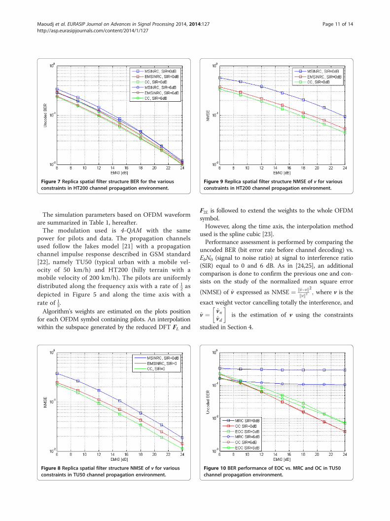
Figure 9 Replica spatial filter structure NMSE of v for variousconstraints in HT200 channel propagation environment.
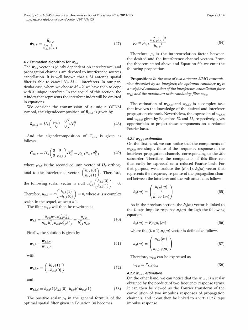
Figure 7 Replica spatial filter structure BER for the variousconstraints in HT200 channel propagation environment.
Maoudj et al. EURASIP Journal on Advances in Signal Processing 2014, 2014:127 Page 11 of 14http://asp.eurasipjournals.com/content/2014/1/127
The simulation parameters based on OFDM waveformare summarized in Table 1, hereafter.The modulation used is 4-QAM with the same
power for pilots and data. The propagation channelsused follow the Jakes model [21] with a propagationchannel impulse response described in GSM standard[22], namely TU50 (typical urban with a mobile vel-ocity of 50 km/h) and HT200 (hilly terrain with amobile velocity of 200 km/h). The pilots are uniformlydistributed along the frequency axis with a rate of 1
2 asdepicted in Figure 5 and along the time axis with arate of 1
5.Algorithm's weights are estimated on the plots position
for each OFDM symbol containing pilots. An interpolationwithin the subspace generated by the reduced DFT FL and
Figure 8 Replica spatial filter structure NMSE of v for variousconstraints in TU50 channel propagation environment.
F2L is followed to extend the weights to the whole OFDMsymbol.However, along the time axis, the interpolation method
used is the spline cubic [23].Performance assessment is performed by comparing the
uncoded BER (bit error rate before channel decoding) vs.EbN0 (signal to noise ratio) at signal to interference ratio(SIR) equal to 0 and 6 dB. As in [24,25], an additionalcomparison is done to confirm the previous one and con-sists on the study of the normalized mean square error
(NMSE) of v expressed as NMSE ¼ v−vk kvk k2
2; where v is the
exact weight vector cancelling totally the interference, and
v ¼ vnvd
� is the estimation of v using the constraints
studied in Section 4.
Figure 10 BER performance of EOC vs. MRC and OC in TU50channel propagation environment.
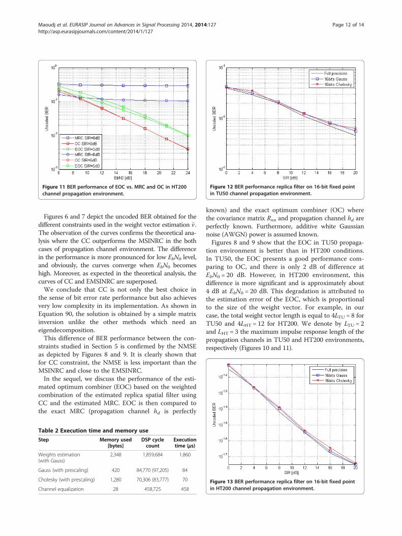
Figure 11 BER performance of EOC vs. MRC and OC in HT200channel propagation environment.
Figure 12 BER performance replica filter on 16-bit fixed pointin TU50 channel propagation environment.
Maoudj et al. EURASIP Journal on Advances in Signal Processing 2014, 2014:127 Page 12 of 14http://asp.eurasipjournals.com/content/2014/1/127
Figures 6 and 7 depict the uncoded BER obtained for thedifferent constraints used in the weight vector estimation v.The observation of the curves confirms the theoretical ana-lysis where the CC outperforms the MSINRC in the bothcases of propagation channel environment. The differencein the performance is more pronounced for low EbN0 level,and obviously, the curves converge when EbN0 becomeshigh. Moreover, as expected in the theoretical analysis, thecurves of CC and EMSINRC are superposed.We conclude that CC is not only the best choice in
the sense of bit error rate performance but also achievesvery low complexity in its implementation. As shown inEquation 90, the solution is obtained by a simple matrixinversion unlike the other methods which need aneigendecomposition.This difference of BER performance between the con-
straints studied in Section 5 is confirmed by the NMSEas depicted by Figures 8 and 9. It is clearly shown thatfor CC constraint, the NMSE is less important than theMSINRC and close to the EMSINRC.In the sequel, we discuss the performance of the esti-
mated optimum combiner (EOC) based on the weightedcombination of the estimated replica spatial filter usingCC and the estimated MRC. EOC is then compared tothe exact MRC (propagation channel hd is perfectly
Table 2 Execution time and memory use
Step Memory used[bytes]
DSP cyclecount
Executiontime (μs)
Weights estimation(with Gauss)
2,348 1,859,684 1,860
Gauss (with prescaling) 420 84,770 (97,205) 84
Cholesky (with prescaling) 1,280 70,306 (83,777) 70
Channel equalization 28 458,725 458
known) and the exact optimum combiner (OC) wherethe covariance matrix Rnn and propagation channel hd areperfectly known. Furthermore, additive white Gaussiannoise (AWGN) power is assumed known.Figures 8 and 9 show that the EOC in TU50 propaga-
tion environment is better than in HT200 conditions.In TU50, the EOC presents a good performance com-paring to OC, and there is only 2 dB of difference atEbN0 = 20 dB. However, in HT200 environment, thisdifference is more significant and is approximately about4 dB at EbN0 = 20 dB. This degradation is attributed tothe estimation error of the EOC, which is proportionalto the size of the weight vector. For example, in ourcase, the total weight vector length is equal to 4LTU = 8 forTU50 and 4LHT = 12 for HT200. We denote by LTU = 2and LHT = 3 the maximum impulse response length of thepropagation channels in TU50 and HT200 environments,respectively (Figures 10 and 11).
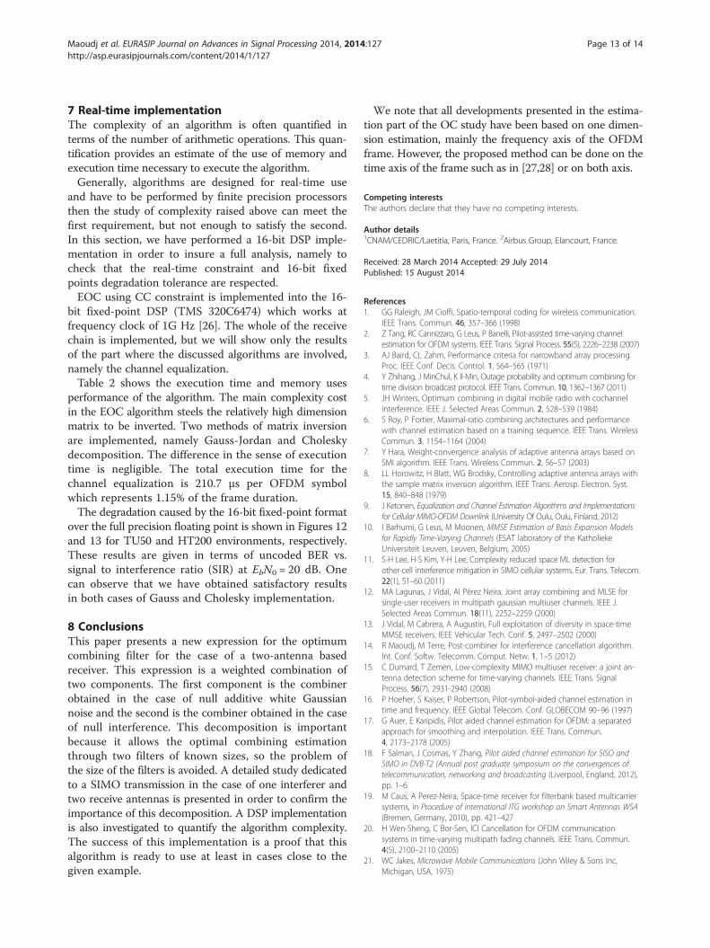
Figure 13 BER performance replica filter on 16-bit fixed pointin HT200 channel propagation environment.
Maoudj et al. EURASIP Journal on Advances in Signal Processing 2014, 2014:127 Page 13 of 14http://asp.eurasipjournals.com/content/2014/1/127
7 Real-time implementationThe complexity of an algorithm is often quantified interms of the number of arithmetic operations. This quan-tification provides an estimate of the use of memory andexecution time necessary to execute the algorithm.Generally, algorithms are designed for real-time use
and have to be performed by finite precision processorsthen the study of complexity raised above can meet thefirst requirement, but not enough to satisfy the second.In this section, we have performed a 16-bit DSP imple-mentation in order to insure a full analysis, namely tocheck that the real-time constraint and 16-bit fixedpoints degradation tolerance are respected.EOC using CC constraint is implemented into the 16-
bit fixed-point DSP (TMS 320C6474) which works atfrequency clock of 1G Hz [26]. The whole of the receivechain is implemented, but we will show only the resultsof the part where the discussed algorithms are involved,namely the channel equalization.Table 2 shows the execution time and memory uses
performance of the algorithm. The main complexity costin the EOC algorithm steels the relatively high dimensionmatrix to be inverted. Two methods of matrix inversionare implemented, namely Gauss-Jordan and Choleskydecomposition. The difference in the sense of executiontime is negligible. The total execution time for thechannel equalization is 210.7 μs per OFDM symbolwhich represents 1.15% of the frame duration.The degradation caused by the 16-bit fixed-point format
over the full precision floating point is shown in Figures 12and 13 for TU50 and HT200 environments, respectively.These results are given in terms of uncoded BER vs.signal to interference ratio (SIR) at EbN0 = 20 dB. Onecan observe that we have obtained satisfactory resultsin both cases of Gauss and Cholesky implementation.
8 ConclusionsThis paper presents a new expression for the optimumcombining filter for the case of a two-antenna basedreceiver. This expression is a weighted combination oftwo components. The first component is the combinerobtained in the case of null additive white Gaussiannoise and the second is the combiner obtained in the caseof null interference. This decomposition is importantbecause it allows the optimal combining estimationthrough two filters of known sizes, so the problem ofthe size of the filters is avoided. A detailed study dedicatedto a SIMO transmission in the case of one interferer andtwo receive antennas is presented in order to confirm theimportance of this decomposition. A DSP implementationis also investigated to quantify the algorithm complexity.The success of this implementation is a proof that thisalgorithm is ready to use at least in cases close to thegiven example.
We note that all developments presented in the estima-tion part of the OC study have been based on one dimen-sion estimation, mainly the frequency axis of the OFDMframe. However, the proposed method can be done on thetime axis of the frame such as in [27,28] or on both axis.
Competing interestsThe authors declare that they have no competing interests.
Author details1CNAM/CEDRIC/Laetitia, Paris, France. 2Airbus Group, Elancourt, France.
Received: 28 March 2014 Accepted: 29 July 2014Published: 15 August 2014
References1. GG Raleigh, JM Cioffi, Spatio-temporal coding for wireless communication.
IEEE Trans. Commun. 46, 357–366 (1998)2. Z Tang, RC Cannizzaro, G Leus, P Banelli, Pilot-assisted time-varying channel
estimation for OFDM systems. IEEE Trans. Signal Process. 55(5), 2226–2238 (2007)3. AJ Baird, CL Zahm, Performance criteria for narrowband array processing.
Proc. IEEE Conf. Decis. Control. 1, 564–565 (1971)4. Y Zhihang, J MinChul, K Il-Min, Outage probability and optimum combining for
time division broadcast protocol. IEEE Trans. Commun. 10, 1362–1367 (2011)5. JH Winters, Optimum combining in digital mobile radio with cochannel
interference. IEEE J. Selected Areas Commun. 2, 528–539 (1984)6. S Roy, P Fortier, Maximal-ratio combining architectures and performance
with channel estimation based on a training sequence. IEEE Trans. WirelessCommun. 3, 1154–1164 (2004)
7. Y Hara, Weight-convergence analysis of adaptive antenna arrays based onSMI algorithm. IEEE Trans. Wireless Commun. 2, 56–57 (2003)
8. LL Horowitz, H Blatt, WG Brodsky, Controlling adaptive antenna arrays withthe sample matrix inversion algorithm. IEEE Trans. Aerosp. Electron. Syst.15, 840–848 (1979)
9. J Ketonen, Equalization and Channel Estimation Algorithms and Implementationsfor Cellular MIMO-OFDM Downlink (University Of Oulu, Oulu, Finland, 2012)
10. I Barhumi, G Leus, M Moonen, MMSE Estimation of Basis Expansion Modelsfor Rapidly Time-Varying Channels (ESAT laboratory of the KatholiekeUniversiteit Leuven, Leuven, Belgium, 2005)
11. S-H Lee, H-S Kim, Y-H Lee, Complexity reduced space ML detection forother-cell interference mitigation in SIMO cellular systems. Eur. Trans. Telecom.22(1), 51–60 (2011)
12. MA Lagunas, J Vidal, AI Pérez Neira, Joint array combining and MLSE forsingle-user receivers in multipath gaussian multiuser channels. IEEE J.Selected Areas Commun. 18(11), 2252–2259 (2000)
13. J Vidal, M Cabrera, A Augustin, Full exploitation of diversity in space-timeMMSE receivers. IEEE Vehicular Tech. Conf. 5, 2497–2502 (2000)
14. R Maoudj, M Terre, Post-combiner for interference cancellation algorithm.Int. Conf. Softw. Telecomm. Comput. Netw. 1, 1–5 (2012)
15. C Dumard, T Zemen, Low-complexity MIMO multiuser receiver: a joint an-tenna detection scheme for time-varying channels. IEEE Trans. SignalProcess. 56(7), 2931-2940 (2008)
16. P Hoeher, S Kaiser, P Robertson, Pilot-symbol-aided channel estimation intime and frequency. IEEE Global Telecom. Conf. GLOBECOM 90–96 (1997)
17. G Auer, E Karipidis, Pilot aided channel estimation for OFDM: a separatedapproach for smoothing and interpolation. IEEE Trans. Commun.4, 2173–2178 (2005)
18. F Salman, J Cosmas, Y Zhang, Pilot aided channel estimation for SISO andSIMO in DVB-T2 (Annual post graduate symposium on the convergences oftelecommunication, networking and broadcasting (Liverpool, England, 2012),pp. 1–6
19. M Caus, A Perez-Neira, Space-time receiver for filterbank based multicarriersystems, in Procedure of international ITG workshop on Smart Antennas WSA(Bremen, Germany, 2010), pp. 421–427
20. H Wen-Sheng, C Bor-Sen, ICI Cancellation for OFDM communicationsystems in time-varying multipath fading channels. IEEE Trans. Commun.4(5), 2100–2110 (2005)
21. WC Jakes, Microwave Mobile Communications (John Wiley & Sons Inc,Michigan, USA, 1975)

Maoudj et al. EURASIP Journal on Advances in Signal Processing 2014, 2014:127 Page 14 of 14http://asp.eurasipjournals.com/content/2014/1/127
22. COST-207, Digital land mobile radio communications (Final report of theCOST-project 207, Commission Of the European Community, Brussels, 1989)
23. SA Dyer, JS Dyer, Cubic-spline interpolation. 1. IEEE Instrum. Meas. Mag.4(1), 44–46 (2001)
24. MR Raghavendra, S Bhashyam, K Giridar, Interference rejection forparametric channel estimation in reuse-1 cellular OFDM systems. IEEE Trans.Vehicular Tech. 58, 4342–4352 (2009)
25. T Zemen, CF Mecklenbräuker, J Wehinger, RR Müller, Iterative jointtime-variant channel estimation and multi-user detection for MC-CDMA.IEEE Trans. Commun. 5, 1469–1478 (2006)
26. TMS320C6474 Multicore digital signal processor data manual (Rev. H)(Texas Instruments Incorporated, 2001)
27. T Zemen, CF Mecklenbrauker, Time-variant channel estimation usingdiscrete prolate spheroidal sequences. IEEE Trans. Signal Process.53, 3597–3607 (2005)
28. T Zemen, L Bernado, N Czink, Iterative time-variant channel estimationfor 802.11p using generalized discrete prolate spheroidal sequences. IEEEVehicular Tech. Conf. 1, 1222–1233 (2012)
doi:10.1186/1687-6180-2014-127Cite this article as: Maoudj et al.: Spatial filter decomposition forinterference mitigation. EURASIP Journal on Advances in Signal Processing2014 2014:127.
Submit your manuscript to a journal and benefi t from:
7 Convenient online submission
7 Rigorous peer review
7 Immediate publication on acceptance
7 Open access: articles freely available online
7 High visibility within the fi eld
7 Retaining the copyright to your article
Submit your next manuscript at 7 springeropen.com