research paper - stt.msu.edumcubed/lmmzl.pdf · research paper numerical methods for solving ......

Author'

s Cop

yRESEARCH PAPER

NUMERICAL METHODS FOR SOLVINGTHE MULTI-TERM TIME-FRACTIONAL

WAVE-DIFFUSION EQUATION

Fawang Liu 1, Mark M. Meerschaert 2,Robert J. McGough 3, Pinghui Zhuang 4, Qingxia Liu 5

Abstract

In this paper, the multi-term time-fractional wave-diffusion equationsare considered. The multi-term time fractional derivatives are defined inthe Caputo sense, whose orders belong to the intervals [0,1], [1,2), [0,2),[0,3), [2,3) and [2,4), respectively. Some computationally effective numer-ical methods are proposed for simulating the multi-term time-fractionalwave-diffusion equations. The numerical results demonstrate the effective-ness of theoretical analysis. These methods and techniques can also beextended to other kinds of the multi-term fractional time-space modelswith fractional Laplacian.

MSC 2010 : 26A33 (main), 65M22, 35L05, 35J05Key Words and Phrases: multi-term time fractional wave-diffusion equa-

tions, Caputo derivative, a power law wave equation, finite difference method,fractional predictor-corrector method

Editorial Note: The first author Fawang Liu received the ”Mittag-Leffler Award: FDA Achievement Award” at the 2012 Symposium on Frac-tional Differentiation and Its Applications (FDA’2012), Hohai University,Nanjing.

1. Introduction

Generalized fractional partial differential equations have been used fordescribing important physical phenomena (see [1, 2, 10, 11, 14, 23, 24, 27]).However, studies of the multi-term time-fractional wave equations are stillunder development.

c© 2013 Diogenes Co., Sofiapp. 9–25 , DOI: 10.2478/s13540-013-0002-2

Author'

s Cop

y

10 F. Liu, M.M. Meerschaert, R.J. McGough, P. Zhuang, Q. Liu

The time fractional diffusion and wave-diffusion equations can be writ-ten in the following form:

Dαt u(x, t) = k

∂2u(x, t)∂x2

+ f(x, t), 0 < x < L, t > 0, (1.1)

where x and t are the space and time variables, k is an arbitrary positiveconstant, f(x, t) is a sufficiently smooth function, 0 < α ≤ 2 and Dα

t is aCaputo fractional derivative of order α defined as [28]

Dαt u(t) =

⎧⎪⎨⎪⎩

1Γ(m − α)

∫ t

0

u(m)(τ)(t − τ)1+α−m

, m − 1 < α < m,

dm

dtmu(t), α = m ∈ N.

When 0 < α < 1, equation (1.1) is a fractional diffusion equation andwhen 1 < α < 2, it is the time fractional diffusion-wave equation. Whenα = 1, equation (1.1) represents a traditional diffusion equation; while ifα = 2, it represents a traditional wave equation. Papers [5, 6, 37] alsodiscussed fractional differential equations with multi-orders. However, inthem multi-orders lying in (0, 2) are only considered.

In order to model loss, the underlying processes cannot be describedby equation (1.1), but can be modelled using its generalization the multi-term time-fractional diffusion-wave and diffusion equations that are givenby [22], namely

Pα,α1,··· ,αn(Dt)u(x, t) = Lx(u(x, t)) + f(x, t), (1.2)where

Pα,α1,··· ,αn(Dt)u(x, t) = (Dαt +

n∑i=1

diDαit )u(x, t), (1.3)

0 < αn < . . . < α1 < α ≤ 1, and di ∈ R, i = 1, . . . , n, n ∈ N ; Dαit is a

Caputo fractional derivative of order αi with respect to t. The operatorLx(u(x, t)) is the well-known linear elliptic differential operator of the sec-ond order. Zhang et al. [36] considered the two-term mobile/immobile timefractional advection-dispersion equation and two-term time fractional wave-diffusion equation. Based on an appropriate maximum principle, Luchko[22] proved the uniqueness and existence results. By the attempts to de-scribe some real processes with the equations of the fractional order, severalresearchers were confronted with the situation that the order α of the frac-tional derivative from the corresponding model equations did not remaininteger and changed, say, in the intervals from 0 to 1, from 1 to 2, from 0to 2 or even from 0 to 4, see for example [4, 15, 13, 34].

Stojanovic [32] found solutions for the fractional wave-diffusion problemin one dimension with n-term time fractional derivatives whose orders be-long to the intervals (0, 1), (1, 2) and (0, 2), respectively, using the methodof the approximation of the convolution by Laguerre polynomials in thespace of tempered distributions.

Author'

s Cop

y

NUMERICAL METHODS FOR SOLVING . . . 11

Time domain wave-equations for lossy media obey a frequency power-law. Frequency-dependent loss and dispersion are typically modeled witha power-law attenuation coefficient, where the power-law exponent rangesfrom 0 to 2. Mathematically, the power-law frequency dependence of theattenuation coefficient cannot be modeled with standard dissipative partialdifferential equations with integer-order derivatives. The generalized time-fractional diffusion equation corresponds to a continuous time random walkmodel where the characteristic waiting time elapsing between two succes-sive jumps diverge, but the accumulated jump length variance remainsfinite and is proportional to tα. The exponent α of the mean square dis-placement proportional to tα often does not remain constant and changes.To adequately describe these phenomena with fractional models, multi-term time-fractional wave-diffusion equations and several approaches havebeen suggested in the literature (for example, [12, 13, 22]). The multi-termtime-fractional wave-diffusion equations successfully capture this power-lawfrequency dependence.

Kelly et al. [13] modified the Szabo wave equation [4, 15, 34]:

�p − 1c20

∂2t p − 2α0

c0 cos(πy/2)∂y+1

t p = 0, (1.4)

adding a second time-fractional term to arrive at the power law wave equa-tion

1c20

∂2t p +

2α0

c0 cos(πy/2)∂y+1

t p +α2

0

cos2(πy/2)∂2y

t p = �p, (1.5)

where 0 ≤ y < 1 or 1 < y ≤ 2; �p =∑

j∂2p∂x2

j. For small α0, the additional

term is negligible, leading to an approximate solution to the Szabo waveequation (1.4). The Riemann-Liouville fractional derivative ∂y

t p = 0Dyt p of

order y (0 ≤ m − 1 < y < m) is defined as (see [28]):

0Dyt p(t) =

1Γ(m − y)

dm

dtm

∫ t

0

p(τ)dτ

(t − τ)α+1−m.

The power law wave equation is used to model sound wave propagationin anisotropic media that exhibits frequency dependent attenuation. Thewave amplitude A falls off exponentially with radial distance r from thesource, so that A = e−α(ω)r where the attenuation coefficient α(ω) dependson the frequency. In human tissue, experimental evidence indicates thatα(ω) = α0|ω|y is a power law, and the exponent y lies in the interval1 ≤ y ≤ 1.5, see for example Duck [8]. It is easy to check, using transformmethods, that the point source solution of (1.5) reproduces this powerlaw attenuation [26]. Some additional properties of the power law waveequation are discussed in [33].

Author'

s Cop

y


Some authors have discussed numerical approximations for fractionalpartial differential equations. Paper [16] considered the space fractionalFokker-Planck equation with instantaneous source and presented a frac-tional method of lines. [25] developed numerical methods to solve theone-dimensional equation with variable coefficients on a finite domain. [29]investigated the numerical approximation of the variational solution onbounded domains in R

2 and presented a method for approximating thesolution in two spatial dimensions using the finite element method. [20]presented a random walk model for approximating a Levy-Feller advection-dispersion process, and proposed an explicit finite difference approximation.[17] considered a space-time fractional advection dispersion equation on afinite domain and proposed implicit and explicit difference methods to solvethis equation. [18] considered a modified anomalous subdiffusion equationwith a nonlinear source term. An implicit difference method is constructed.Its stability and convergence are discussed using the energy method, [18].[38] proposed explicit and implicit Euler approximations for the variable-order fractional advection-diffusion equation with a nonlinear source term.Stability and convergence of the methods are discussed. [9] proposed anadvanced implicit meshless approach for the non-linear anomalous subdif-fusion equation. [21] also proposed an implicit RBF meshless approach fortime fractional diffusion equations.

Numerical solutions of the multi-term time-fractional wave-diffusionequations (MT-TFWDE) with the fractional orders lying in (0, n)(n > 2)are still limited. The main purpose of this paper is to derive numerical solu-tions of the multi-term time-fractional wave-diffusion equations with nonho-mogeneous Dirichlet boundary conditions. The multi-term time-fractionalderivatives are defined in the Caputo sense, whose orders belong to theintervals [0, 1], [1, 2), [0, 2), [0, 3), [2, 3) and [2, 4), respectively. The Caputoand Riemann-Liouville forms are related through the boundary conditions(see Remark 3). As far as we know there are no relevant research papersin the published literature that cover all of these cases.

The rest of this paper is organized as follows. Two implicit numeri-cal methods for simulating the two-term mobile/immobile time-fractionaldiffusion equation and the two-term time-fractional wave-diffusion equa-tion are proposed in Sections 2 and 3, respectively. Two computationallyeffective fractional predictor-corrector methods for the multi-term time-fractional wave-diffusion equations are investigated in Section 4. Finally,some examples are discussed to illustrate the application of our theoreticalresults.

Author'

s Cop

y


2. A two-term mobile/immobile time-fractionaladvection-dispersion equation

In order to distinguish explicitly the mobile and immobile status usingfractional dynamics, [30] developed the fractional-order, mobile/immobilemodel for the total concentration, i.e., the following two-term mobile/immobiletime-fractional diffusion equation, whose orders belong to the intervals [0,1]:

a2∂C(x, t)

∂t+ a1

∂γC(x, t)∂tγ

= D∂2C(x, t)

∂x2+ f(x, t), (2.1)

with initial condition:

C(x, 0) = ϕ0(x), (2.2)

and boundary conditions:

C(a, t) = φ1(t), C(b, t) = φ2(t), 0 ≤ t ≤ T, (2.3)

where a1 > 0, a2 > 0, 0 < γ < 1, D > 0.We define tk = kτ, k = 0, 1, . . . , n; xi = a + ih, i = 0, 1, . . . ,m, where

τ = T/n and h = (b − a)/m are space and time step sizes, respectively.We discretize the Caputo time-fractional derivative as (see [31])

∂γC(x, tk+1)∂tγ

=1

Γ(1 − γ)

k∑j=0

∫ tj+1

tj

∂C(x,η)∂η

(tk+1 − η)γdη (2.4)

=k∑

j=0

C(x, tj+1) − C(x, tj)Γ(1 − γ)τ

∫ tj+1

tj

dη

(tk+1 − η)γ+ O(τ2−γ)

=τ−γ

Γ(2 − γ)

k∑j=0

bγj [C(x, tk+1−j) − C(xi, tk−j)] + O(τ2−γ),

where bγj = (j + 1)1−γ − j1−γ , j = 0, 1, 2, · · · , n.

Hence, we have

a2C(xi, tk+1) − C(xi, tk)

τ

+a1τ

−γ

Γ(2 − γ)

k∑j=0

bγj [C(xi, tk+1−j) − C(xi, tk−j)] (2.5)

= DC(xi−1, tk+1) − 2C(xi, tk+1) + C(xi+1, tk+1)

h2

+ f(xi, tk+1) + Ri,k+1

where

|Ri,k+1| ≤ K(τ + τ2−α + h). (2.6)

Author'

s Cop

y


Let Cki be the numerical approximation to C(xi, tk), then we obtain the

following implicit difference approximation of equations (2.1)-(2.3):

a2Ci,k+1 − Ci,k

τ+

a1τ−γ

Γ(2 − γ)

k∑j=0

bγj [Ci,k+1−j − Ci,k−j]

= DCi−1,k+1 − 2Ci,k+1 + Ci+1,k+1

h2+ fi,k+1. (2.7)

The initial and boundary conditions are discretized as follows

Ci,0 = ϕ(xi), i = 0, 1, 2, . . . ,m, (2.8)C0,k = φ1(kτ), Cm,k = φ2(kτ), k = 1, 2, . . . , n. (2.9)

Theorem 1. The fractional implicit numerical method defined by(2.7), (2.8) and (2.9) is unconditionally stable.

P r o o f. Using similar techniques as in [19], we can prove this result.

Theorem 2. Let Ci,k be the numerical solution computed by use ofthe implicit numerical methods (2.7)-(2.9), C(x, t) is the exact solution ofthe problem (2.1)-(2.3). Then there is a positive constant C , such that

|Ci,k − C(xi, tk)| ≤ C(τ + τ2−α + h), (2.10)where i = 1, 2, · · · ,m − 1; k = 1, 2, . . . , n.

P r o o f. Using similar techniques in [19], we can prove this result.

3. A two-term time-fractional wave-diffusion equation

A two-term time fractional wave-diffusion model with damping withindex 1 < γ = 1 + γ < 2 and whose orders belong to the intervals [1,2) canbe written as the following form:

a2∂γC(x, t)

∂tγ+ a1

∂C(x, t)∂t

= D∂2C(x, t)

∂x2+ f(x, t), (3.1)

with initial condition:

C(x, 0) = ϕ0(x),∂C(x, 0)

∂t= ϕ1(x), a ≤ x ≤ b, (3.2)

and boundary conditions:C(a, t) = φ1(t), C(b, t) = φ2(t), 0 ≤ t ≤ T, (3.3)

where a1 > 0, a2 > 0 and D > 0.This partial differential equation with γ = 2 is called the telegraph

equation which governs electrical transmission in a telegraph cable. It canalso be characterized as a fractional diffusion-wave equation (which governswave motion in a string) with a damping effect due to the terms 1 < γ < 2and a1

∂C(x,t)∂t in equation (3.1).

Author'

s Cop

y


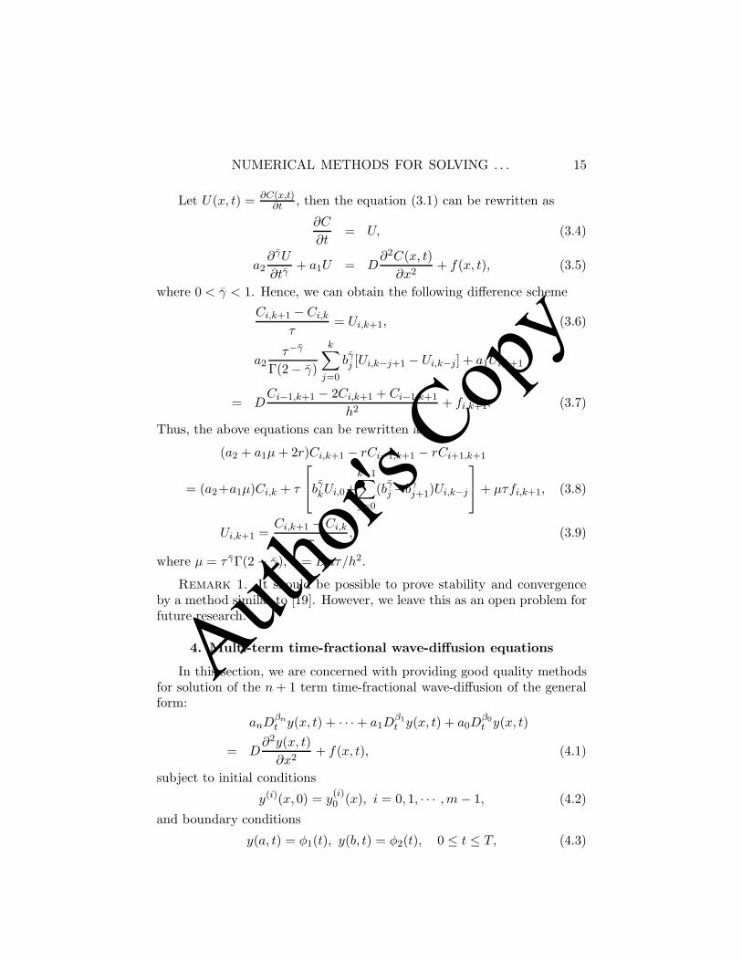
Let U(x, t) = ∂C(x,t)∂t , then the equation (3.1) can be rewritten as

∂C

∂t= U, (3.4)

a2∂γU

∂tγ+ a1U = D

∂2C(x, t)∂x2

+ f(x, t), (3.5)

where 0 < γ < 1. Hence, we can obtain the following difference schemeCi,k+1 − Ci,k

τ= Ui,k+1, (3.6)

a2τ−γ

Γ(2 − γ)

k∑j=0

bγj [Ui,k−j+1 − Ui,k−j] + a1Ui,k+1

= DCi−1,k+1 − 2Ci,k+1 + Ci−1,k+1

h2+ fi,k+1. (3.7)

Thus, the above equations can be rewritten as

(a2 + a1μ + 2r)Ci,k+1 − rCi−1,k+1 − rCi+1,k+1

= (a2+a1μ)Ci,k + τ

⎡⎣bγ

kUi,0+k−1∑j=0

(bγj −bγ

j+1)Ui,k−j

⎤⎦ + μτfi,k+1, (3.8)

Ui,k+1 =Ci,k+1 − Ci,k

τ, (3.9)

where μ = τ γΓ(2 − γ), r = Dμτ/h2.

Remark 1. It should be possible to prove stability and convergenceby a method similar to [19]. However, we leave this as an open problem forfuture research.

4. Multi-term time-fractional wave-diffusion equations

In this section, we are concerned with providing good quality methodsfor solution of the n + 1 term time-fractional wave-diffusion of the generalform:

anDβnt y(x, t) + · · · + a1D

β1t y(x, t) + a0D

β0t y(x, t)

= D∂2y(x, t)

∂x2+ f(x, t), (4.1)

subject to initial conditions

y(i)(x, 0) = y(i)0 (x), i = 0, 1, · · · ,m − 1, (4.2)

and boundary conditions

y(a, t) = φ1(t), y(b, t) = φ2(t), 0 ≤ t ≤ T, (4.3)

Author'

s Cop

y


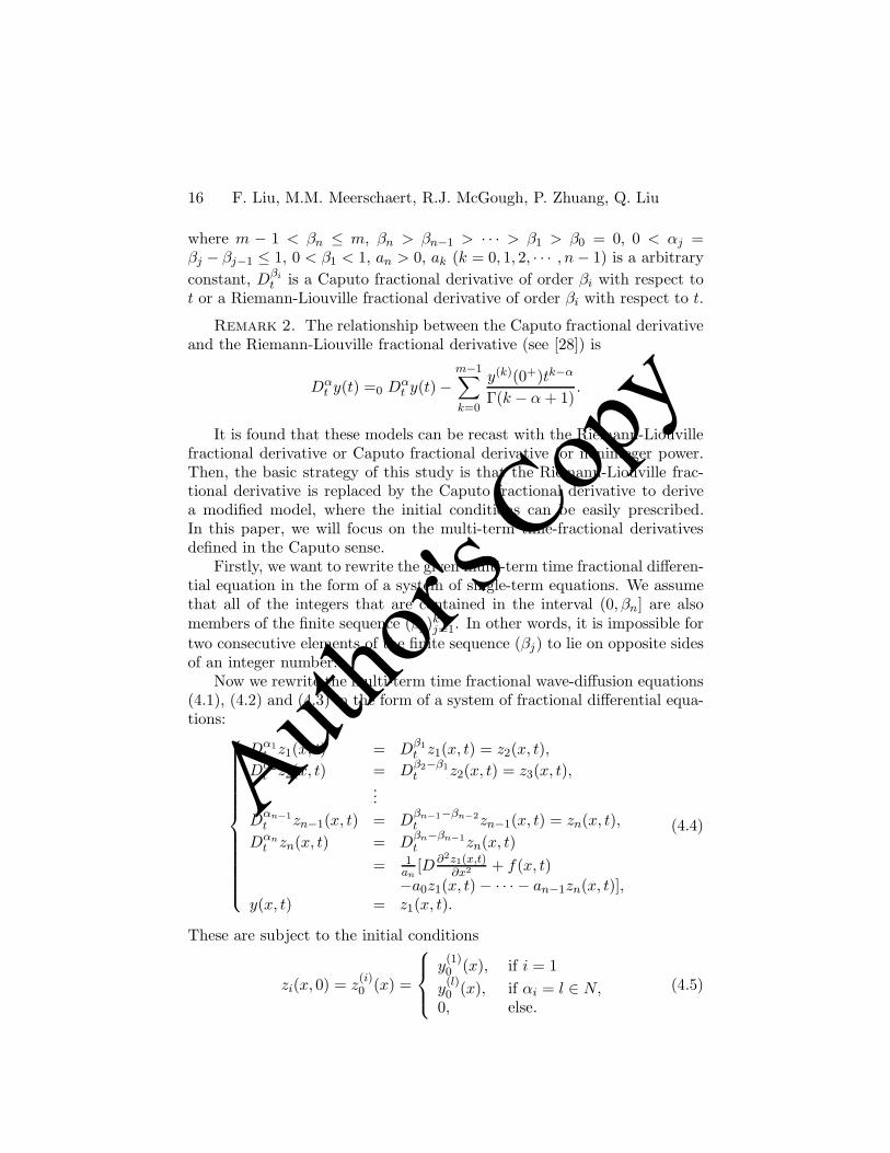
where m − 1 < βn ≤ m, βn > βn−1 > · · · > β1 > β0 = 0, 0 < αj =βj − βj−1 ≤ 1, 0 < β1 < 1, an > 0, ak (k = 0, 1, 2, · · · , n − 1) is a arbitraryconstant, Dβi

t is a Caputo fractional derivative of order βi with respect tot or a Riemann-Liouville fractional derivative of order βi with respect to t.

Remark 2. The relationship between the Caputo fractional derivativeand the Riemann-Liouville fractional derivative (see [28]) is

Dαt y(t) =0 Dα

t y(t) −m−1∑k=0

y(k)(0+)tk−α

Γ(k − α + 1).

It is found that these models can be recast with the Riemann-Liouvillefractional derivative or Caputo fractional derivative for noninteger power.Then, the basic strategy of this study is that the Riemann-Liouville frac-tional derivative is replaced by the Caputo fractional derivative to derivea modified model, where the initial conditions can be easily prescribed.In this paper, we will focus on the multi-term time-fractional derivativesdefined in the Caputo sense.

Firstly, we want to rewrite the given multi-term time fractional differen-tial equation in the form of a system of single-term equations. We assumethat all of the integers that are contained in the interval (0, βn] are alsomembers of the finite sequence (βj)kj=1. In other words, it is impossible fortwo consecutive elements of the finite sequence (βj) to lie on opposite sidesof an integer number.

Now we rewrite the multi-term time fractional wave-diffusion equations(4.1), (4.2) and (4.3) in the form of a system of fractional differential equa-tions:⎧⎪⎪⎪⎪⎪⎪⎪⎪⎪⎪⎪⎪⎨

⎪⎪⎪⎪⎪⎪⎪⎪⎪⎪⎪⎪⎩

Dα1t z1(x, t) = Dβ1

t z1(x, t) = z2(x, t),Dα2

t z2(x, t) = Dβ2−β1t z2(x, t) = z3(x, t),

...D

αn−1t zn−1(x, t) = D

βn−1−βn−2t zn−1(x, t) = zn(x, t),

Dαnt zn(x, t) = D

βn−βn−1t zn(x, t)

= 1an

[D ∂2z1(x,t)∂x2 + f(x, t)

−a0z1(x, t) − · · · − an−1zn(x, t)],y(x, t) = z1(x, t).

(4.4)

These are subject to the initial conditions

zi(x, 0) = z(i)0 (x) =

⎧⎪⎨⎪⎩

y(1)0 (x), if i = 1

y(l)0 (x), if αi = l ∈ N,

0, else.(4.5)

Author'

s Cop

y


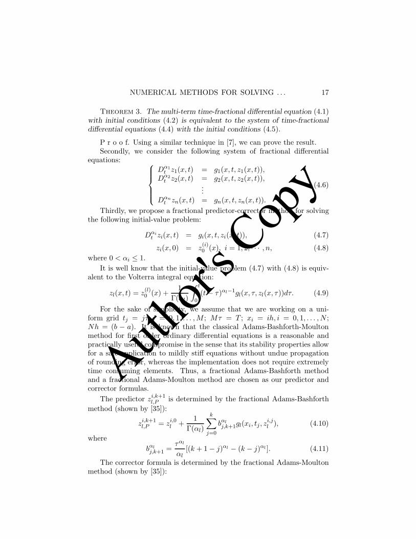
Theorem 3. The multi-term time-fractional differential equation (4.1)with initial conditions (4.2) is equivalent to the system of time-fractionaldifferential equations (4.4) with the initial conditions (4.5).

P r o o f. Using a similar technique in [7], we can prove the result.Secondly, we consider the following system of fractional differential

equations: ⎧⎪⎪⎪⎨⎪⎪⎪⎩

Dα1t z1(x, t) = g1(x, t, z1(x, t)),

Dα2t z2(x, t) = g2(x, t, z2(x, t)),

...Dαn

t zn(x, t) = gn(x, t, zn(x, t)).

(4.6)

Thirdly, we propose a fractional predictor-corrector method for solvingthe following initial-value problem:

Dαit zi(x, t) = gi(x, t, zi(x, t)), (4.7)

zi(x, 0) = z(i)0 (x), i = 1, 2, · · · , n, (4.8)

where 0 < αi ≤ 1.It is well know that the initial-value problem (4.7) with (4.8) is equiv-

alent to the Volterra integral equation:

zl(x, t) = z(l)0 (x) +

1Γ(αl)

∫ t

0(t − τ)αl−1gl(x, τ, zl(x, τ))dτ. (4.9)

For the sake of simplicity, we assume that we are working on a uni-form grid tj = jτ, j = 0, 1, . . . ,M ; Mτ = T ; xi = ih, i = 0, 1, . . . , N ;Nh = (b − a). It is known that the classical Adams-Bashforth-Moultonmethod for first order ordinary differential equations is a reasonable andpractically useful compromise in the sense that its stability properties allowfor a safe application to mildly stiff equations without undue propagationof rounding error, whereas the implementation does not require extremelytime consuming elements. Thus, a fractional Adams-Bashforth methodand a fractional Adams-Moulton method are chosen as our predictor andcorrector formulas.

The predictor zi,k+1l,P is determined by the fractional Adams-Bashforth

method (shown by [35]):

zi,k+1l,P = zi,0

l +1

Γ(αl)

k∑j=0

bαlj,k+1gl(xi, tj , z

i,jl ), (4.10)

wherebαlj,k+1 =

ταl

αl[(k + 1 − j)αl − (k − j)αl ]. (4.11)

The corrector formula is determined by the fractional Adams-Moultonmethod (shown by [35]):

Author'

s Cop

y


zi,k+1l = zi,0

l +1

Γ(αl)(4.12)

×⎛⎝ k∑

j=0

aαlj,k+1gl(xi, tj, z

i,jl ) + aαl

k+1,k+1gl(xi, tk+1, zi,k+1l,P )

⎞⎠ ,

where

aαlj,k+1 =

ταl

αl(αl + 1)

×

⎧⎪⎪⎨⎪⎪⎩

kαl+1 − (k − αl)(k + 1)αl , j = 0,(k − j + 2)αl+1 + (k − j)αl+1

−2(k − j + 1)αl+1, 1 ≤ j ≤ k,1, j = k + 1.

(4.13)

The above numerical techniques are used to solve the system of frac-tional differential equations in ((4.4) and (4.5).

The predictor zi,k+1l,P is determined by the fractional Adams-Bashforth

method (l = 1, · · · , n − 1):

zi,k+1l,P = zi,0

l +1

Γ(αl)

k∑j=0

bαlj,k+1z

i,jl+1, (4.14)

zi,k+1n,P = zi,0

n +1

Γ(αn)

k∑j=0

bαnj,k+1[

zi+1,j1 − 2zi,j

1 + zi−1,j1

h2

+ fi,j − a1zi,j2 − · · · ,−an−1z

i,jn ]. (4.15)

The corrector formula is determined by the fractional Adams-Moultonmethod (l = 1, · · · , n − 1):

zi,k+1l = zi,0

l +1

Γ(αl)

⎛⎝ k∑

j=0

aαlj,k+1z

i,jl+1 + aαi

k+1,k+1zi,k+1l+1,P ,

⎞⎠ , (4.16)

zi,k+1n = zi,0

n +1

anΓ(αn){

k∑j=0

aαnj,k+1[

zi+1,j1 − 2zi,j

1 + zi−1,j1

h2

+ fi,j − a1zi,j2 − · · · − an−1z

i,jn ]

+ aαnk+1,k+1[

zi+1,k+11,P − 2zi,k+1

1,P + zi−1,k+11,P

h2

+ fi,k+1 − a1zi,k+12,P − · · · − an−1z

i,k+1n,P ]}. (4.17)

Author'

s Cop

y


We note that∂2z(xi, tk+1)

∂x2=

z(xi+1, tk+1) − 2z(xi, tk+1) + z(xi−1, tk+1)h2

+ O(h2), (4.18)

∂z(xi, tk+1)∂t

=z(xi, tk+1) − z(xi, tk)

τ+ O(τ). (4.19)

If all αl ∈ (0, 1), we call the fractional predictor-corrector methods(4.14)-(4.16) with (4.17) as FPCM-1. If some αl = 1, then we replacethe fractional predictor-corrector methods (4.14)-(4.16) with the followingmethod

zi,k+1l = zi,k

l + τzi,k+1l+1 , (4.20)

which is called FPCM-2.Thus, we have the following results.

Theorem 4. For FPCM-1, we have the following error estimation:

max0 < i < N1 < k < M

|zl(xi, tk) − zi,kl | = O(τ q + h2), (4.21)

where q = 1 + min αl.

Theorem 5. For FPCM-2, we have the following error estimation:

max0 < i < N1 < k < M

|zl(xi, tk) − zi,kl | = O(τ q + τ + h2). (4.22)

5. Numerical results

In order to illustrate the practical application of our numerical methods,some examples are presented.

Example 1. Consider the following two-term time fractional diffusionequation:

∂C(x, t)∂t

+∂γC(x, t)

∂tγ=

∂2C(x, t)∂x2

+ f(x, t), (5.1)

together with the following boundary and initial conditions{C(0, t) = t2, C(1, t) = et2, 0 ≤ t ≤ 1,C(x, 0) = 0, 0 ≤ x ≤ 1 (5.2)

where 0 < γ < 1 and f(x, t) = (2t − t2 + 2t2−γ

Γ(3−γ))ex.

The exact solution of the equations (5.1) and (5.2) is u(x, t) = t2ex.From Table 1, we can observe that

‖E‖max ≤ C(τ + h2).

Author'

s Cop

y


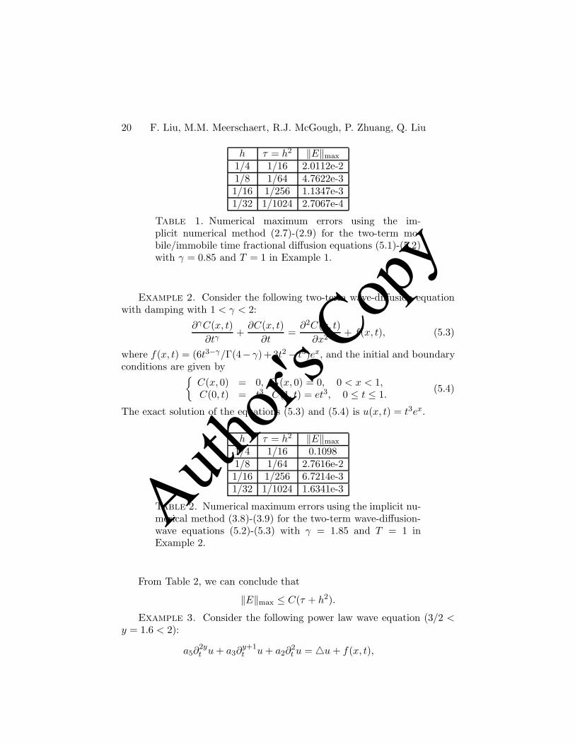
h τ = h2 ‖E‖max

1/4 1/16 2.0112e-21/8 1/64 4.7622e-31/16 1/256 1.1347e-31/32 1/1024 2.7067e-4

Table 1. Numerical maximum errors using the im-plicit numerical method (2.7)-(2.9) for the two-term mo-bile/immobile time fractional diffusion equations (5.1)-(5.2)with γ = 0.85 and T = 1 in Example 1.

Example 2. Consider the following two-term wave-diffusion equationwith damping with 1 < γ < 2:

∂γC(x, t)∂tγ

+∂C(x, t)

∂t=

∂2C(x, t)∂x2

+ f(x, t), (5.3)

where f(x, t) = (6t3−γ/Γ(4− γ)+3t2 − t3)ex, and the initial and boundaryconditions are given by{

C(x, 0) = 0, Ct(x, 0) = 0, 0 < x < 1,C(0, t) = t3, C(1, t) = et3, 0 ≤ t ≤ 1. (5.4)

The exact solution of the equations (5.3) and (5.4) is u(x, t) = t3ex.

h τ = h2 ‖E‖max

1/4 1/16 0.10981/8 1/64 2.7616e-21/16 1/256 6.7214e-31/32 1/1024 1.6341e-3

Table 2. Numerical maximum errors using the implicit nu-merical method (3.8)-(3.9) for the two-term wave-diffusion-wave equations (5.2)-(5.3) with γ = 1.85 and T = 1 inExample 2.

From Table 2, we can conclude that

‖E‖max ≤ C(τ + h2).

Example 3. Consider the following power law wave equation (3/2 <y = 1.6 < 2):

a5∂2yt u + a3∂

y+1t u + a2∂

2t u = �u + f(x, t),

Author'

s Cop

y


where a2 = 1c20

, a3 = 2α0c0 cos(πy/2) , a5 = α2

0cos2(πy/2)

,

f(x, t) = [a5Γ(6)

Γ(6 − 2y)t5−2y +

a3Γ(6)Γ(5 − y)

t4−y + 20a2t3 − t5]ex.

Initial and boundary conditions:

u(x, 0) = ut(x, 0) = utt(x, 0) = 0, (5.5)

u(0, t) = t5, u(1, t) = et5. (5.6)

The exact solution is u(x, t) = t5ex.

h τ = h2 FPCM-2 FPCM-11/4 1/16 0.3664 0.17111/8 1/64 0.1110 4.9093e-21/16 1/256 3.3093e-2 1.0323e-21/32 1/1024 9.3205e-3 2.01235e-3

Table 3. Numerical maximum errors using the Predictor-Corrector method (FPCM-1 and FPCM-2) for the powerlow equation y = 1.6 in Example 3.

From Table 3, we can conclude that

‖E‖max ≤ C(τ + τ1+min αl + h2), in FPCM − 2;

‖E‖max ≤ C(τ1+min αl + h2), in FPCM − 1.

6. Conclusion

In this paper, some computationally effective numerical methods areproposed for simulating the two-term mobile/immobile time-fractional dif-fusion equation, the two-term time-fractional wave-diffusion equation andtwo computationally effective fractional predictor-corrector methods for themulti-term time-fractional wave-diffusion equations. The numerical resultsdemonstrate the effectiveness of theoretical analysis.

Acknowledgements

This research has been supported by the Australian Research Coun-cil grant DP1094333, USA NSF grants DMS-1025486, DMS-0803360, NIHgrant R01-EB012079, China NSF grants 11101344 and Fujian NSF grants2010J01011.

Author'

s Cop

y


References

[1] B. Baeumer and M.M. Meerschaert, Stochastic solutions for fractionalCauchy problems. Fract. Calc. Appl. Anal. 4, No 4 (2001), 481–500.

[2] B. Baeumer, S. Kurita and M.M. Meerschaert, Inhomogeneous frac-tional diffusion eqautions. Fract. Calc. Appl. Anal., 8, No 4 (2005),371–376; at http://www.math.bas.bg/∼fcaa.

[3] D. Bolster, M.M. Meerschaert and A. Sikorskii, Product rule for vectorfractional derivatives. Fract. Calc. Appl. Anal. 15, No 3 (2012), 463–478; DOI:10.2478/s13540-012-0033-0;at http://link.springer.com/article/10.2478/s13540-012-0033-0.

[4] W. Chen, S. Holm, Modified Szabo’s wave equation models for lossymedia obeying frequency power law. J. Acoust. Soc. Am. 114 (2003),2570–2754.

[5] W. Deng, C. Li, Q. Guo, Analysis of fractional differential equationswith multi-orders. Fractals 15, No 2 (2007), 173–182.

[6] W. Deng, C. Li, J. Lu, Stability analysis of linear fractional differentialsystem with multiple time-delays. Nonlinear Dynamics 48, No 4 (2007),409–416.

[7] K. Diethelm, The Analysis of Fractional Differential Equations.Springer, Berlin etc. (2010).

[8] F.A. Duck, Physical Properties of Tissue: A Comprehensive ReferenceBook. Academic Press (1990).

[9] Y. Gu, P. Zhuang, F. Liu, An advanced implicit meshless approach forthe non-linear anomalous subdiffusion equation. Computer Modeling inEng. & Sciences 56 (2010), 303–334.

[10] M. Ilic, F. Liu, I. Turner, V. Anh, Numerical approximation of afractional-in-space diffusion equation (I). Fract. Calc. Appl. Anal., 8,No 3 (2005), 323–341; at http://www.math.bas.bg/∼fcaa.

[11] M. Ilic, F. Liu, I. Turner, V. Anh, Numerical approximation ofa fractional-in-space diffusion equation (II) – with nonhomogeneousboundary conditions. Fract. Calc. Appl. Anal., 9, No 4 (2006), 333–349; at http://www.math.bas.bg/∼fcaa.

[12] H. Jiang, F. Liu, I. Turner, K. Burrage, Analytical solutions forthe multi-term time-space Caputo-Riesz fractional advection-diffusionequations on a finite domain. J. Math. Anal. Appl. 389 (2012), 1117–1127.

[13] J.K. Kelly, R.J. McGough, M.M. Meerschaert, Analytical time-domainGreen’s functions for power-law media. J. Acoust. Soc. Am. 124 (2008),2861–2872.

[14] C. Li, F. Zeng, F. Liu, Spectral approximations to the frac-tional integral and derivative. Fract. Calc. Appl. Anal. 15, No 3

http://www.math.bas.bg/~fcaa

http://link.springer.com/article/10.2478/s13540-012-0033-0



Author'

s Cop

y


(2012), 383–406; DOI:10.2478/s13540-012-0028-x;at http://link.springer.com/article/10.2478/s13540-012-0028-x

[15] M. Liebler, S. Ginter, T. Dreyer, R.E. Riedlinger, Full wave model-ing of therapeutic ultrasound: Efficient time-domain implementation ofthe frequency power-law attenuation. J. Acoust. Soc. Am. 116 (2004),2742–2750.

[16] F. Liu, V. Anh, I. Turner, Numerical solution of the space fractionalFokker-Planck equation. J. Comp. Appl. Math. 166 (2004), 209–219.

[17] F. Liu, P. Zhuang, V. Anh, I. Turner, K. Burrag, Stability and conver-gence of the difference methods for the space-time fractional advection-diffusion equation. J. Comp. Appl. Math. 191 (2007), 12–20.

[18] F. Liu, C. Yang, K. Burrage, Numerical method and analytical tech-nique of the modified anomalous subdiffusion equation with a nonlinearsource term. J. Comp. Appl. Math. 231 (2009), 160–176.

[19] F. Liu, P. Zhuang, K. Burrage, Numerical methods and analysis for aclass of fractional advection-dispersion models. Computers and Math.with Appl. 63 (2012), 1–22.

[20] Q. Liu, F. Liu, I. Turner, V. Anh, Approximation of the Levy-Feller advection-dispersion process by random walk and finite differencemethod. J. Comp. Phys. 222 (2007), 57–70.

[21] Q. Liu, Y. Gu, P. Zhuang, F. Liu, Y. Nie, An implicit RBF meshlessapproach for time fractional diffusion equations. Comput. Mech. 48(2011), 1–12.

[22] Y. Luchko, Initial-boundary-value problems for the generalized multi-term time-fractional diffusion equation. J. Math. Anal. Appl. 374(2011), 538–548.

[23] M.M. Meerschaert and H.P. Scheffler, Semistable Levy motion. Fract.Calc. Appl. Anal., 5, No 1 (2002), 27–54.

[24] M.M. Meerschaert, J. Mortensen, H.P. Scheffler, Vector Grunwald for-mula for fractional derivatives. Fract. Calc. Appl. Anal. 7, No 1 (2004),61–82.

[25] M.M. Meerschaert, C. Tadjeran, Finite difference approximations forfractional advection-dispersion flow equations. J. Comp. Appl. Math.172 (2004), 65–77.

[26] M.M. Meerschaert, P. Straka, Y. Zhou, R.J. McGough, Stochastic so-lution to a time-fractional attenuated wave equation. Nonlinear Dy-namics 70 (2012), 1273–1281.

[27] R. Metzler, J. Klafter, The random walk’s guide to anomalous diffu-sion: a fractional dynamics approach. Phys. Rep. 339 (2000), 1–77.

[28] I. Podlubny, Fractional Differential Equations. Academic Press, NewYork (1999).

http://link.springer.com/article/10.2478/s13540-012-0028-x

Author'

s Cop

y


[29] J.P. Roop, Computational aspects of FEM approximation of fractionaladvection dispersion equations on bounded domains in R

2. J. Comp.Appl. Math. 193 (2006), 243–268.

[30] R. Schumer, D.A. Benson, M.M Meerschaert, B. Baeumer, Fractal mo-bile/immobile solute transport. Water Resources Researces 39 (2003),1296–1307.

[31] S. Shen, F. Liu, V. Anh, Numerical approximations and solution tech-niques for the space-time Riesz-Caputo fractional advection-diffusionequation. Numerical Algorithm 56 (2011), 383–404.

[32] M. Stojanovic, Numerical method for solving diffusion-wave phenom-ena. J. Comp. Appl. Math. 235 (2011), 3121–3137.

[33] P. Straka, M.M. Meerschaert, R.J. McGough, and Y. Zhou, Fractionalwave equations with attenuation. Fract. Calc. Appl. Anal. 16, No 1(2013), 262–272 (same issue); DOI:10.2478/s13540-013-0016-9;at http://link.springer.com/journal/13540.

[34] T.L. Szabo, Time domain wave equations for lossy media obeying afrequency power law. J. Acoust. Soc. Am. 96 (1994), 491–500.

[35] C. Yang, F. Liu, A computationally effective predictor-correctormethod for simulating fractional order dynamical control system.ANZIAM J. 47 (2006), 168–184.

[36] Y. Zhang, D.A. Benson, D.M. Reeves, Time and space nonlocalities un-derlying fractional-derivative models: Distinction and literature reviewof field applications. Advances in Water Resources 32 (2009), 561–581.

[37] F. Zhang, C. Li, Stability analysis of fractional differential systemswith order lying in (1,2). Advances in Difference Equations (2011), ID213485.

[38] P. Zhuang, F. Liu, V. Anh, I. Turner, Numerical methods for thevariable order fractional advection diffusion equation with a nonlinearsource term. SIAM J. Numer. Anal. 47 (2009), 1760–1781.

1 School of Mathematical SciencesQueensland University of TechnologyGPO Box 2434, Brisbane, Qld. 4001, AUSTRALIA

e-mail: [email protected] Received: June 11, 2012

2 Department of Statistics and ProbabilityMichigan State UniversityEast Lansing, Michigan – 48824, USA

e-mail: [email protected]

http://link.springer.com/journal/13540

Author'

s Cop

y


3 Department of Electrical and Computer EngineeringMichigan State UniversityEast Lansing, Michigan – 48824, USA

e-mail: [email protected]

4,5 School of Mathematical SciencesXiamen University, Xiamen 361005, P.R. CHINA

e-mails: [email protected], [email protected]

Please cite to this paper as published in:Fract. Calc. Appl. Anal., Vol. 16, No 1 (2013), pp. 9–25;DOI: 10.2478/s13540-013-0002-2

research paper - stt.msu.edumcubed/lmmzl.pdf · research paper numerical methods for solving ......

Documents