research project submission (copy and paste).pdf
TRANSCRIPT
Seediscussions,stats,andauthorprofilesforthispublicationat:http://www.researchgate.net/publication/267777098
KineticModellingandReactorDesignMethanolSynthesis2013
THESIS·APRIL2013
DOI:10.13140/2.1.3571.0407
DOWNLOADS
127
VIEWS
139
1AUTHOR:
KelvinOba
AstonUniversity
1PUBLICATION0CITATIONS
SEEPROFILE
Availablefrom:KelvinOba
Retrievedon:15July2015
Kinetic Modelling and Reactor Design Methanol Synthesis
2013
Kelvin Obareti CE4005
4/26/2013
CE4005 | Abstract 1
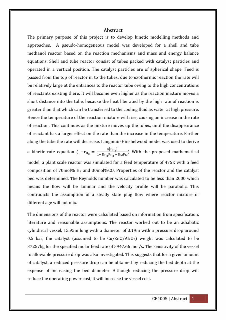
Abstract The primary purpose of this project is to develop kinetic modelling methods and
approaches. A pseudo-homogeneous model was developed for a shell and tube
methanol reactor based on the reaction mechanisms and mass and energy balance
equations. Shell and tube reactor consist of tubes packed with catalyst particles and
operated in a vertical position. The catalyst particles are of spherical shape. Feed is
passed from the top of reactor in to the tubes; due to exothermic reaction the rate will
be relatively large at the entrances to the reactor tube owing to the high concentrations
of reactants existing there. It will become even higher as the reaction mixture moves a
short distance into the tube, because the heat liberated by the high rate of reaction is
greater than that which can be transferred to the cooling fluid as water at high pressure.
Hence the temperature of the reaction mixture will rise, causing an increase in the rate
of reaction. This continues as the mixture moves up the tubes, until the disappearance
of reactant has a larger effect on the rate than the increase in the temperature. Farther
along the tube the rate will decrease. Langmuir-Hinshelwood model was used to derive
a kinetic rate equation ( [ ]
) With the proposed mathematical
model, a plant scale reactor was simulated for a feed temperature of 475K with a feed
composition of 70mol% H2 and 30mol%CO. Properties of the reactor and the catalyst
bed was determined. The Reynolds number was calculated to be less than 2000 which
means the flow will be laminar and the velocity profile will be parabolic. This
contradicts the assumption of a steady state plug flow where reactor mixture of
different age will not mix.
The dimensions of the reactor were calculated based on information from specification,
literature and reasonable assumptions. The reactor worked out to be an adiabatic
cylindrical vessel, 15.95m long with a diameter of 3.19m with a pressure drop around
0.5 bar, the catalyst (assumed to be Cu/ZnO/Al2O3) weight was calculated to be
37257kg for the specified molar feed rate of 5947.66 mol/s. The sensitivity of the vessel
to allowable pressure drop was also investigated. This suggests that for a given amount
of catalyst, a reduced pressure drop can be obtained by reducing the bed depth at the
expense of increasing the bed diameter. Although reducing the pressure drop will
reduce the operating power cost, it will increase the vessel cost.
CE4005 | Abstract 2
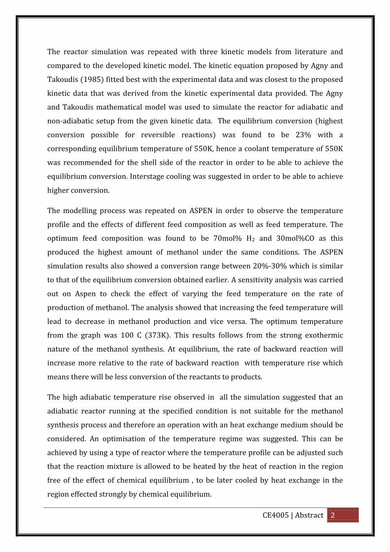
The reactor simulation was repeated with three kinetic models from literature and
compared to the developed kinetic model. The kinetic equation proposed by Agny and
Takoudis (1985) fitted best with the experimental data and was closest to the proposed
kinetic data that was derived from the kinetic experimental data provided. The Agny
and Takoudis mathematical model was used to simulate the reactor for adiabatic and
non-adiabatic setup from the given kinetic data. The equilibrium conversion (highest
conversion possible for reversible reactions) was found to be 23% with a
corresponding equilibrium temperature of 550K, hence a coolant temperature of 550K
was recommended for the shell side of the reactor in order to be able to achieve the
equilibrium conversion. Interstage cooling was suggested in order to be able to achieve
higher conversion.
The modelling process was repeated on ASPEN in order to observe the temperature
profile and the effects of different feed composition as well as feed temperature. The
optimum feed composition was found to be 70mol% H2 and 30mol%CO as this
produced the highest amount of methanol under the same conditions. The ASPEN
simulation results also showed a conversion range between 20%-30% which is similar
to that of the equilibrium conversion obtained earlier. A sensitivity analysis was carried
out on Aspen to check the effect of varying the feed temperature on the rate of
production of methanol. The analysis showed that increasing the feed temperature will
lead to decrease in methanol production and vice versa. The optimum temperature
from the graph was 100 C (373K). This results follows from the strong exothermic
nature of the methanol synthesis. At equilibrium, the rate of backward reaction will
increase more relative to the rate of backward reaction with temperature rise which
means there will be less conversion of the reactants to products.
The high adiabatic temperature rise observed in all the simulation suggested that an
adiabatic reactor running at the specified condition is not suitable for the methanol
synthesis process and therefore an operation with an heat exchange medium should be
considered. An optimisation of the temperature regime was suggested. This can be
achieved by using a type of reactor where the temperature profile can be adjusted such
that the reaction mixture is allowed to be heated by the heat of reaction in the region
free of the effect of chemical equilibrium , to be later cooled by heat exchange in the
region effected strongly by chemical equilibrium.
CE4005 | Abstract 3
Table of Contents Abstract ..................................................................................................................................... 1
1. Introduction ...................................................................................................................... 7
2. Background ....................................................................................................................... 7
2.1. Available Process Routes .......................................................................................... 8
2.2. Reactor Model Description ..................................................................................... 12
3. Literature Review ........................................................................................................... 15
3.1. Process Description ................................................................................................. 15
3.2. Reaction Mechanisms and Kinetic Models ............................................................ 18
3.2.1. Mechanisms involving CO ................................................................................ 18
3.2.2. Mechanisms Involving CO2 ............................................................................. 19
3.3. Thermodynamic Equilibrium ................................................................................. 20
3.4. Selectivity ................................................................................................................. 22
3.5. Catalysts ................................................................................................................... 23
3.5.1. High-pressure Catalysts ................................................................................... 23
3.5.2. Low-pressure Catalysts ................................................................................... 24
3.6. Kinetic Models .......................................................................................................... 26
3.6.1. Natta et al (1953) ............................................................................................. 27
3.6.2. Rozovskii (1980) and Klier (1982) ................................................................ 27
3.6.3. Agny and Takoudis (1985) .............................................................................. 28
3.6.4. Skrzypek's (1985 and 1991) ........................................................................... 29
3.6.5. Lim (2009) ........................................................................................................ 31
3.6.6. Literature Review Conclusion ......................................................................... 34
4. Work Plan and Methodology ......................................................................................... 35
4.1. To develop a kinetic model for the synthesis of methanol from the synthetic
rate data given in Appendix 1 ........................................................................................... 35
4.1.1. Developing Langmuir-Hinshelwood Kinetic Model from Experimental Data
35
4.1.2. Experimental Data Incorporated into Kinetic Model From Literature ........ 36
4.2. Simulating a Plant-Scale Catalytic Reactor ............................................................ 39
4.2.1. Reactor Volume ................................................................................................ 40
4.2.2. Reactor Length and Diameter ......................................................................... 40
CE4005 | Abstract 4
4.2.3. Reactor Dome Closure ..................................................................................... 41
4.2.4. Catalyst Bed Characteristics ............................................................................ 42
4.3. Sensitivity to pressure drop ................................................................................... 43
4.4. Effect of Coolant Temperature ................................................................................... 43
4.5. Modelling with ASPEN Process Modelling Software. ........................................... 44
4.6. Gantt Chart ............................................................................................................... 44
5. Results and Discussion .................................................................................................. 44
5.1. Developing a kinetic model from experimental data ........................................... 44
5.1.1. Dependence on the product methanol ........................................................... 46
5.1.2. Dependence on Carbon Monoxide .................................................................. 47
5.1.3. Dependence on Hydrogen ............................................................................... 47
5.1.4. Finding k and K Values ..................................................................................... 48
5.2. Plant-Scale Catalytic Reactor Simulation ............................................................... 51
5.2.1. Reactor Dimension ........................................................................................... 59
5.3. Experimental Data Incorporated Into Kinetic Models from Literature .............. 66
5.4. Effect of Coolant Temperatures .............................................................................. 74
5.5. Modelling with ASPEN Process Modelling Software ............................................ 76
5.6. Further Discussion .................................................................................................. 81
6. Conclusion ....................................................................................................................... 82
7. Recommendations .......................................................................................................... 84
8. Nomenclature ................................................................................................................. 86
9. References ....................................................................................................................... 87
10. Appendices
10.1 Appendix 1: Data for Kinetic Analysis
10.2 Appendix 2: Possible Routes to Methanol
10.3 Appendix 3: Deriving non-adiabatic energy balance
10.4 Appendix 4: ASPEN Simulation Results
10.5 Appendix 5: Improved Gantt Chart
10.6 Appendix 6: Reactor Simulation Summary
10.7 Appendix 7: USB stick with ASPEN and Microsoft Excel Simulation and
Graphs
CE4005 | Abstract 5
List of Figures Figure 1 Structural formula of methanol ................................................................................... 7
Figure 2. The ICI-steam-raising reactor for low-pressure methanol synthesis [iv]. ................ 10
Figure 3 Simplified route to methanol production [].............................................................. 11
Figure 4 Production of methanol from atmospheric carbon dioxide or from neutral gas
(methane), and its use as a fuel. DMFC: direct methanol fuel cell [i]. .................................... 11
Figure 5 Schematic diagram of a plug flow reactor ................................................................. 12
Figure 6 Mass balance around a plug flow reactor ................................................................. 12
Figure 7. Essential process steps in Lurgi’s Low Pressure Methanol Process []. ..................... 16
Figure 8. Flow sheet of Lurgi's Methanol Synthesis Loop [xii] ................................................. 17
Figure 9. Thermodynamics of methanol synthesis. Variation of equilibrium constant kp with
temperature and pressure [iv] ................................................................................................. 21
Figure 10. Reaction temperature profile of adiabatic and non-adiabatic set up at conversion
between 0 and 0.9 ................................................................................................................... 59
Figure 11. Reactor hemispherical dome closure dimension ................................................... 61
Figure 12. Preliminary dimension of the plant-scale catalytic reactor .................................... 62
Figure 13. Reactor dimension sensitivity to pressure drop ..................................................... 66
Figure 14. Reaction rate as a function of degree of conversion in the adiabatic reactor. ...... 71
Figure 15. Relationship between temperature and degree of conversion in the adiabatic
reactor. ..................................................................................................................................... 71
Figure 16. Reaction rate as a function of degree of conversion in the non-adiabatic reactor.
.................................................................................................................................................. 73
Figure 17. Relationship between temperature and degree of conversion in the non-adiabatic
reactor. ..................................................................................................................................... 73
Figure 18. Plot of equilibrium conversion as a function of temperature. ............................... 75
Figure 19. Interstage cooling []. ............................................................................................... 76
Figure 20. Reactor model summary ......................................................................................... 77
Figure 21. Flow sheet with heat and material balance for ASPEN simulation at a feed inlet
temperature of 473K (200 C) ................................................................................................... 78
Figure 22. Temperature profile of the reactor at a feed composition of 70% H2 and 30% CO
.................................................................................................................................................. 79
Figure 23. Sensitivity of methanol production to different feed temperatures. ................... 80
CE4005 | Abstract 6
List of Tables Table 1. Catalysts proposed or used for industrial process [iv]. .............................................. 23
Table 2. Important rate expressions for methanol synthesis []. ............................................. 26
Table 3. Elementary Reactions for Cu/ZnO/Al2O3/ZrO2 catalysed methanol synthesis [] ....... 32
Table 4. Reaction rates for methanol synthesis reaction and DME production [xxvi]. ........... 33
Table 5. Methanol synthesis kinetic models to be compared to developed kinetic model .... 34
Table 6. Data for Kinetic Analysis ............................................................................................. 45
Table 7. Experiment 1 compared to experiment 5. ................................................................. 46
Table 8. Experiments to deduce the dependence on carbon monoxide ................................ 47
Table 9. Effect of decreasing the partial pressure of hydrogen on the rate of reaction. ........ 47
Table 10. Constant hydrogen partial pressure for kinetic parameter ..................................... 49
Table 11. Constant methanol partial pressure for kinetic parameter ..................................... 50
Table 12. Experimental data table modified to include values of VO , CA0, FA0 and ṁ ........... 55
Table 13. Experiment 12 reaction conditions 1 ....................................................................... 57
Table 14. Experiment 12 reaction conditions 2 ...................................................................... 57
Table 15. Reactor volume and temperature profiles for adiabatic and non-adiabatic setup at
conversion between 0 and 0.9................................................................................................. 58
Table 16. Summary of reactor cylindrical section dimension.................................................. 60
Table 17. Summary of overall rector dimension ..................................................................... 62
Table 18. Summary of catalyst bed characteristics. ................................................................ 64
Table 19. Reactor dimension sensitivity to pressure drop ...................................................... 65
Table 20. Methanol synthesis kinetic models and rate equation............................................ 66
Table 21. Comparison of kinetic model simulation results. .................................................... 67
Table 22. Summary of Agny and Takoudis model for an adiabatic reactor using the provided
experimental data .................................................................................................................... 69
Table 23. Summary of Agny and Takoudis model for non-adiabatic reactor setup using the
experimental data provided .................................................................................................... 72
Table 24. Results table for temperature-conversion relationship. ......................................... 74
CE4005 | Introduction 7
1. Introduction
The primary purpose of this project is to develop a kinetic model for the synthesis of
methanol from given set of synthetic rate data. The result of the kinetic model will then
be used to simulate a shell-and-tube reactor at specified conditions, using a simple one-
dimensional, plug-flow, pseudo homogeneous, nonisothermal reactor model. The
kinetic model developed will be compared to other kinetic models suggested by
literature and the best model will be used in the reactor design and to study the
performance of the reactor. This will provide an opportunity to demonstrate and apply
technical knowledge. Also, the ability in critical analysis will be demonstrated.
2. Background
The issue of sustainability is that which concerns many industries and given the option
of moving from the consumption of fossil fuels towards renewable/cleaner energy
makes the synthesis of methanol very important.
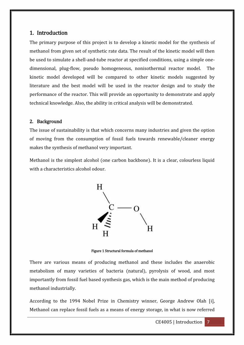
Methanol is the simplest alcohol (one carbon backbone). It is a clear, colourless liquid
with a characteristics alcohol odour.
Figure 1 Structural formula of methanol
There are various means of producing methanol and these includes the anaerobic
metabolism of many varieties of bacteria (natural), pyrolysis of wood, and most
importantly from fossil fuel based synthesis gas, which is the main method of producing
methanol industrially.
According to the 1994 Nobel Prize in Chemistry winner, George Andrew Olah [i],
Methanol can replace fossil fuels as a means of energy storage, in what is now referred
CE4005 | Background 8
to as the methanol economy. Apart from the current use of methanol today as chemical
feedstock for producing useful chemical products like, acetic acid, formaldehyde (used
in construction and wooden boarding) and methyl tert-butyl ether (MBTE), due to its
high octane rating, and biodegradability, methanol can be used directly as a fuel in
hybrid vehicles and as a fuel in fuel cells which are renewable forms of energy
production.
2.1. Available Process Routes
From 1830 up until the mid-1920’s, wood de ived o natu al methanol was the main
source of methanol. The first commercial production of methanol was by the destructive
distillation of wood, hence methanol is sometimes called wood alcohol [ii]. Apart from
wood pyrolysis, there are various means of producing methanol and these includes the
anaerobic metabolism of many varieties of bacteria (natural), and most importantly
from fossil fuel based synthesis gas, which is the main method of producing methanol
industrially [iii].
The synthesis gas that was first used for the production of methanol was manufactured
by coke gasification. In recent times, the synthesis gas is now almost invariably
produced by steam reforming or partial oxidation of hydrocarbons, usually natural gas
[iv].
The production of methanol from synthesis gas occurs in two steps. The first step
involves the conversion of the feedstock natural gas (methane) into a synthesis gas
stream that consists of carbon monoxide (CO), carbon dioxide (CO2), water (H2O) and
hydrogen (H2). The first step is usually carried out by the catalytic steam reforming of
hydrocarbon feedstock or by non-catalytic partial oxidation of hydrocarbon or coal [iii].
Methanol produced via the catalytic hydrogenation of carbon monoxide and/or carbon
dioxide occurs via the three reactions given below [iv].
1. Hydrogenation of carbon monoxide:
CO + 2H2 CH3OH (ΔH298K = -90.64kJ/mol, ΔG°= -25.34kJ/mol) (2.1)
2. Hydrogenation of carbon dioxide:
CO2 + 3H2 CH3OH + H2O (ΔH298K = -49.47kJ/mol, ΔG°= +3.30kJ/mol) (2.2)
CE4005 | Background 9
3. Water-gas shift reaction:
CO2 + H2 CO+ H2O (ΔH298K = -41.47kJ/mol, ΔG°= -28.64kJ/mol) (2.3)
Synthetic route for methanol production was first commercialised by BASF in Germany.
The process was based on the reaction of synthesis gas which is a mixture of hydrogen
and carbon oxides. The reaction occurred over a zinc chromite catalyst at relatively high
temperatures of 300 to 400°C and high pressures (250 to 350atm). Synthesis gas was
derived from coal via the water gas reaction [v]. By 1965, a state-of-the-art, high
pressure methanol unit typically had the following characteristics: Capacity, 70 to 150
thousand tonnes per year; Operating pressure, 350atm; Consumption, 11-12 million
kcal per tonne of methanol (130-140 ft3 of natural gas per gallon).
In 1966, Imperial Chemical Industries (ICI) developed the low pressure methanol
synthesis which was a significant breakthrough in methanol technology. The synthesis
was carried out over a proprietary based copper catalyst. This high activity catalyst
allowed the methanol synthesis reaction to proceed at commercially acceptable levels at
relatively low temperatures (220 - 280°C) which allowed operation at a notably
reduced pressure of 50 atm. Overall, the ICI low-pressure was more economical than
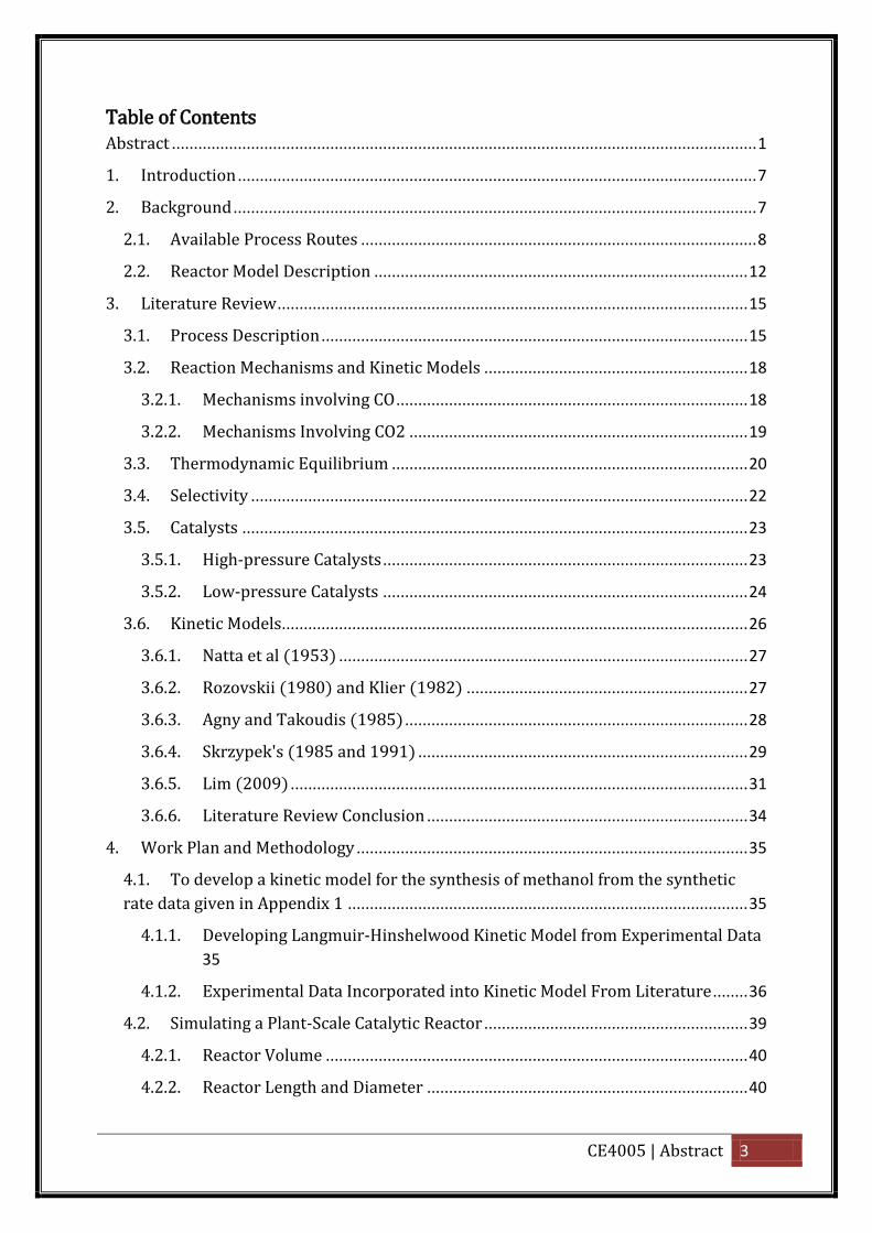
the high pressure system in terms of capital and operating cost [vi]. Figure 2 below
shows the ICI process which uses multi-bed synthesis reactors with feed gas quench
cooling.
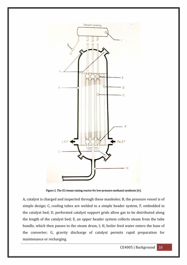
CE4005 | Background 10
Figure 2. The ICI-steam-raising reactor for low-pressure methanol synthesis [iv].
A, catalyst is charged and inspected through these manholes; B, the pressure vessel is of
simple design; C, cooling tubes are welded to a simple header system, F, embedded in
the catalyst bed; D, perforated catalyst support grids allow gas to be distributed along
the length of the catalyst bed; E, an upper header system collects steam from the tube
bundle, which then passes to the steam drum, I; H, boiler feed water enters the base of
the converter; G, gravity discharge of catalyst permits rapid preparation for
maintenance or recharging.
CE4005 | Background 11
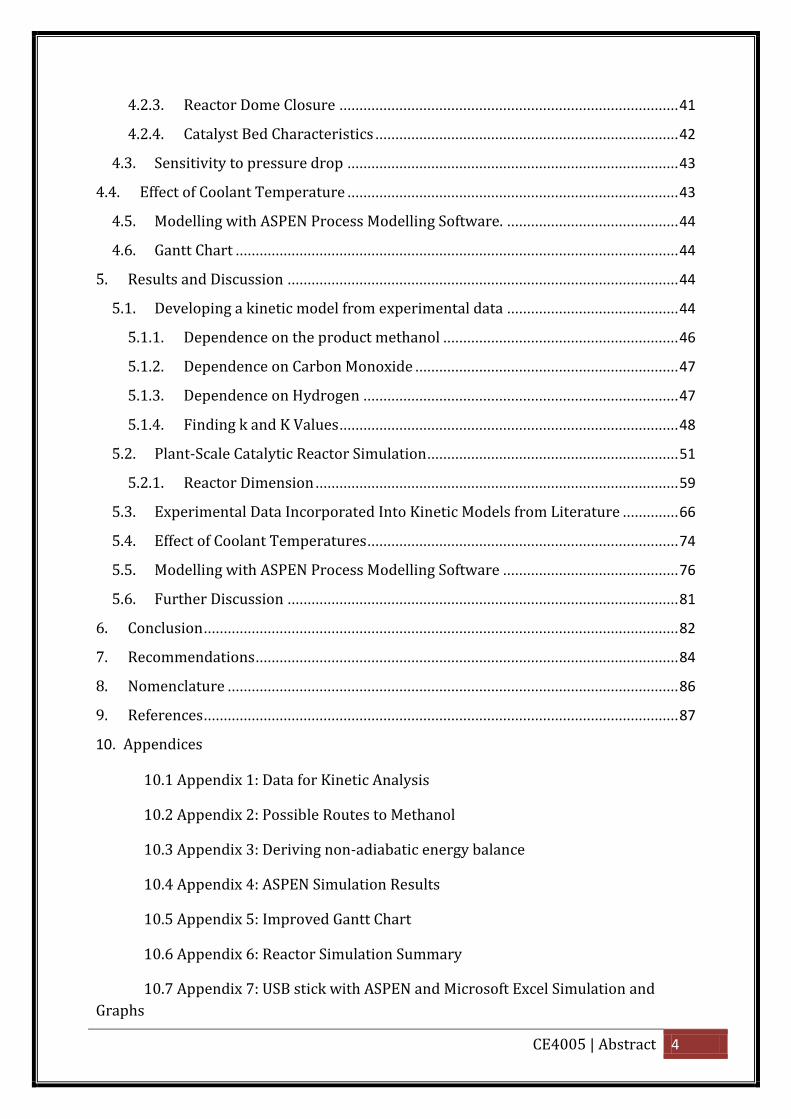
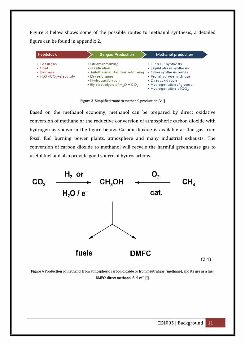
Figure 3 below shows some of the possible routes to methanol synthesis, a detailed
figure can be found in appendix 2.
Figure 3 Simplified route to methanol production [vii]
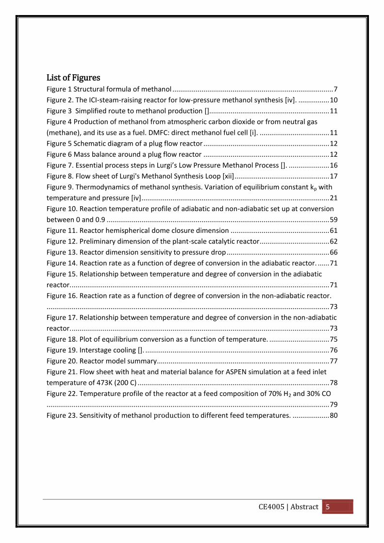
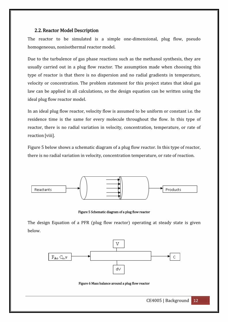
Based on the methanol economy, methanol can be prepared by direct oxidative
conversion of methane or the reductive conversion of atmospheric carbon dioxide with
hydrogen as shown in the figure below. Carbon dioxide is available as flue gas from
fossil fuel burning power plants, atmosphere and many industrial exhausts. The
conversion of carbon dioxide to methanol will recycle the harmful greenhouse gas to
useful fuel and also provide good source of hydrocarbons.
(2.4)
Figure 4 Production of methanol from atmospheric carbon dioxide or from neutral gas (methane), and its use as a fuel.
DMFC: direct methanol fuel cell [i].
CE4005 | Background 12
2.2. Reactor Model Description
The reactor to be simulated is a simple one-dimensional, plug flow, pseudo
homogeneous, nonisothermal reactor model.
Due to the turbulence of gas phase reactions such as the methanol synthesis, they are
usually carried out in a plug flow reactor. The assumption made when choosing this
type of reactor is that there is no dispersion and no radial gradients in temperature,
velocity or concentration. The problem statement for this project states that ideal gas
law can be applied in all calculations, so the design equation can be written using the
ideal plug flow reactor model.
In an ideal plug flow reactor, velocity flow is assumed to be uniform or constant i.e. the
residence time is the same for every molecule throughout the flow. In this type of
reactor, there is no radial variation in velocity, concentration, temperature, or rate of
reaction [viii].
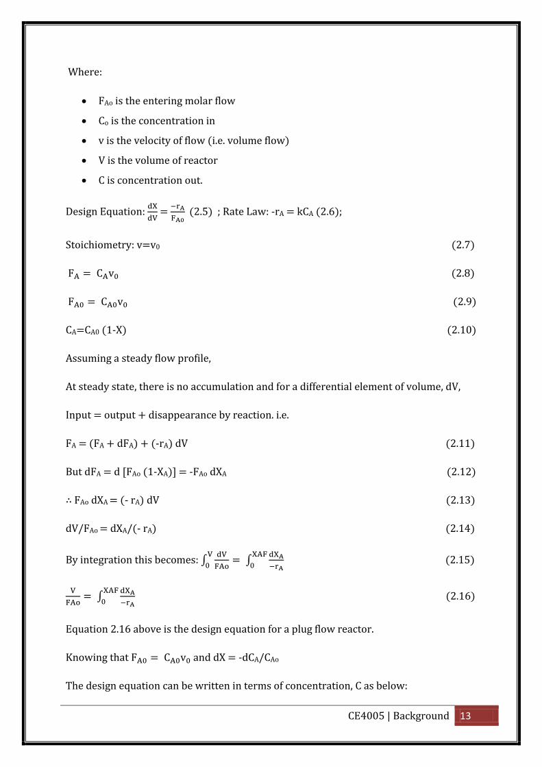
Figure 5 below shows a schematic diagram of a plug flow reactor. In this type of reactor,
there is no radial variation in velocity, concentration temperature, or rate of reaction.
Figure 5 Schematic diagram of a plug flow reactor
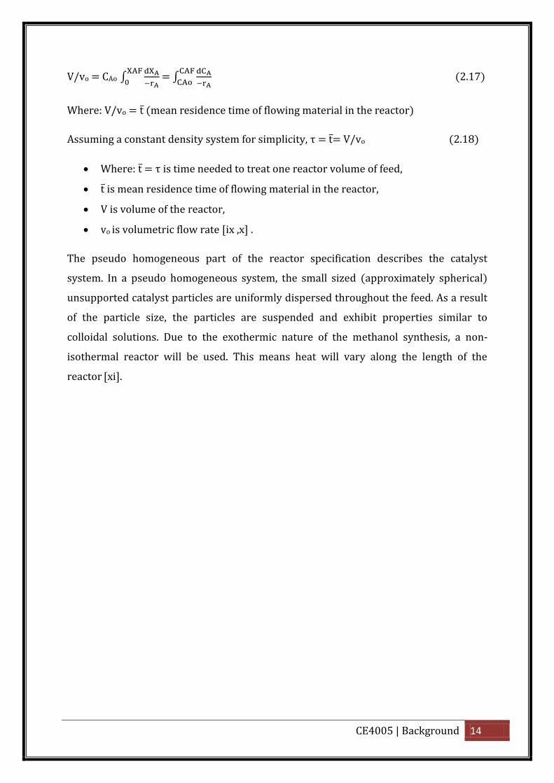
The design Equation of a PFR (plug flow reactor) operating at steady state is given
below.
Figure 6 Mass balance around a plug flow reactor
CE4005 | Background 13
Where:
FAo is the entering molar flow
Co is the concentration in
v is the velocity of flow (i.e. volume flow)
V is the volume of reactor
C is concentration out.
Design Equation:
=
(2. ; Rate Law: -rA = kCA (2.6);
Stoichiometry: v=v0 (2.7)
v (2.8)
v (2.9)
CA=CA0 (1-X) (2.10)
Assuming a steady flow profile,
At steady state, there is no accumulation and for a differential element of volume, dV,
Input = output + disappearance by reaction. i.e.
FA = (FA + dFA) + (-rA) dV (2.11)
But dFA = d [FAo (1-XA)] = -FAo dXA (2.12)
FAo dXA = (- rA) dV (2.13)
dV/FAo = dXA/(- rA) (2.14)
By integration this becomes: ∫
∫
(2.15)
∫
(2.16)
Equation 2.16 above is the design equation for a plug flow reactor.
Knowing that v and dX = -dCA/CAo
The design equation can be written in terms of concentration, C as below:
CE4005 | Background 14
V/vo = CAo ∫
= ∫
(2.17)
Where: V/vo = t (mean residence time of flowing material in the reactor)
Assuming a constant density system for simplicity, τ t= V/vo (2.18)
Where: t = τ is time needed to treat one reactor volume of feed,
t is mean residence time of flowing material in the reactor,
V is volume of the reactor,
vo is volumetric flow rate [ix ,x] .
The pseudo homogeneous part of the reactor specification describes the catalyst
system. In a pseudo homogeneous system, the small sized (approximately spherical)
unsupported catalyst particles are uniformly dispersed throughout the feed. As a result
of the particle size, the particles are suspended and exhibit properties similar to
colloidal solutions. Due to the exothermic nature of the methanol synthesis, a non-
isothermal reactor will be used. This means heat will vary along the length of the
reactor [xi].
CE4005 | Literature Review 15
3. Literature Review
This literature review will cover the methanol production process and some of the
previous kinetic models developed for methanol synthesis. The knowledge of the kinetic
mechanism of a chemical process presents a considerable importance in the reactions
which corresponds to the chemical equilibrium because this alone can allow the design
of the devices and sizing of the appliances needed to remove the heat conducted in
different parts of a reactor. Mathematical models of methanol synthesis are often
valuable tools that can be used in the evaluation of those systems. Any successful kinetic
model must include the rate equations of the reaction that accurately predict the effects
of process variable changes on reactor performance. Linear and nonlinear regression is
a method often used by many researchers to analyse data collected in order to produce
a reaction rate expression [ii]. The rate equations will vary depending on the assumed
mechanism and the role of each reactant in the reaction. In a case where a particular
reactant is weakly adsorbed to the surface of the catalyst used to catalyse the reaction,
such weakly adsorbed reactants are usually left out of the rate equation.
Before discussing the kinetic model, factors affecting the rate of the methanol synthesis
reaction will be discussed. Such factors are:
Reaction mechanism
Thermodynamic equilibrium
Process condition (Temperature, pressure)
Catalysts
3.1. Process Description
The methanol process consists mainly of three parts.
Synthesis gas preparation,
Methanol synthesis, and
Methanol distillation
As discussed earlier, methanol synthesis has improved from using high pressure to low
pressure which is more cost effective. Two low-pressure methanol synthesis processes
dominates the market; the ICI process which uses multi-bed synthesis reactors with
feed gas quench cooling and the Lurgi process [xii] that makes use of multitubular
CE4005 | Literature Review 16
synthesis reactors with internal cooling. The synthesis gas used in the production of
methanol is a mixture of CO, CO2 and H2. This synthesis gas can be produced from
various feedstock such as natural gas, higher hydrocarbons and coal. The synthesis gas
is produced conventionally via the steam reforming process but it can also be produced
from CO2 reforming, partial oxidation and auto thermal reforming. Figure 7 below
shows the essential steps of Lu gi’s Low Pressure Methanol Process with combined
reforming of oil associated natural gas. In the Lurgi reactor with typical operating
conditions of 523 K and 80 bar, the catalyst is packed in vertical tubes surrounded by
boiling water. Reaction heat is transferred to the boiling water to produce steam. Due to
the efficient heat transfer, very little temperature gradient is observed along the reactor.
The pressure of the boiling water helps to control the reactor temperature.
Figure 7. Essential p ocess steps in Lu gi’s Low P essu e Methanol P ocess [xiii].
Natural gas first undergoes desulphurization and gets saturated with process steam
then undergoes three steps of reforming (using Ni-based catalyst.):
Preforming - Higher hydrocarbons are converted to methane by steam reforming
and methanation in an adiabatic reactor
Steam reforming – parts of the methane gas are converted to synthesis gas by
the highly endothermic steam reforming reaction, reaction energy is supplied by
the burning of natural gas outside the catalyst tubes in a multitubular reactor.
Autothermal reforming – The remaining methane is converted into synthesis gas
CE4005 | Literature Review 17
The reactions occurring in the synthesis gas preparation are:
CnHm + nH2O nCO + (
) (3.1)
CH4 + H2O CO + 3H2 (ΔH,298K = -206kJ/mol) (3.2)
CH4 +
CO + 2H2 (ΔH,298K = 35kJ/mol) (3.3)
The water gas shift (equation 3) occurs in all the reforming steps.
In the methanol synthesis, synthesis gas is converted to methanol over a Cu/Zn/Al2O3
catalyst. Figure 8 below shows the Lu gi’s [xii] methanol synthesis loop.
Figure 8. Flow sheet of Lurgi's Methanol Synthesis Loop [xii]
Due to the quasi-isothermal reaction conditions and high catalyst selectivity, only small
amounts of by-products are produced during methanol synthesis. The methanol
synthesis loop consists of two parallel reactors with a common steam drum,
feed/effluent interchanger, a cooler, a methanol separator and a recycle compressor.
The methanol produced needs to be distilled to remove water, dissolved gases and
ethanol. Ethanol is the most difficult component to remove due to the small difference in

CE4005 | Literature Review 18
the volatility between ethanol and methanol. Firstly, the dissolved gases are separated
from the crude methanol by flashing at low pressure. Low and high boiling by-products
are removed in energy integrated three column distillation sequence. Ethanol is
removed in the side stream of the third of these columns [xiii].
3.2. Reaction Mechanisms and Kinetic Models
Two types of reaction mechanisms associated with methanol synthesis are discussed
below.
3.2.1. Mechanisms involving CO
Although many investigators support the carbon monoxide hydrogenation theory, the
source of methanol is still an open question. Is methanol synthesised from carbon
monoxide or carbon dioxide?
Herman et al., [xiv,xv] believes that carbon monoxide is adsorbed (with a carbon-metal
bond) and then successively hydrogenated to form formyl, hydroxycarbene and
hydroxyl-methyl species leading to methanol. Alternatively, Deluzarche et al., [xvi]
suggested that carbon monoxide is inserted into a surface hydroxyl group to form a
surface formate species (with an oxygen-metal bond), followed by hydrogenation and
dehydration to form a surface methoxide that leads to methanol. This mechanism
requires an oxygen bond to an active site. Although ICI investigators documented the
formation of a stable intermediate formate species, Kung et al., analysed the available
data [xvii] from the mechanisms proposed by Herman et al., and Deluzarche et al.,
sufficient evidence was found, which disprove those mechanisms. Kung found evidence
for carbon monoxide adsorption with the carbon end of the molecule towards the metal.
Agny and Takoudis [xviii] reiterated and refined a third mechanism that was proposed
by Henrici-Olive and Olive [xix]. This third mechanism introduced a new intermediate
between the formyl and methoxide species- surface bonded formaldehyde as shown in
equation 3.4 below.
(3.4)
The presence of the surface-bonded formaldehyde was verified by others such as
Tawarah and Hansen [xx] and Edwards and Schrader [xxi].
CE4005 | Literature Review 19
Transmission infrared spectroscopy was used by Edward and Schrader to develop the
mechanism. However, they speculate that the formaldehyde might be formed by carbon
monoxide insertion into an adsorbed hydroxyl group to form a bidentate formate
species. The infrared studies conducted under reaction conditions also showed that the
CO is adsorbed on the Cu(I) sites of the catalyst used, but much of the reaction occurs on
the zinc oxide component [xxi].
3.2.2. Mechanisms Involving CO2
The thermodynamics of the reaction of carbon dioxide to methanol are very
unfavourable at typical reaction conditions. This made Kung et al. reach a conclusion
that it is very unlikely for any proposed mechanism involving carbon dioxide
hydrogenation to be the predominant one [xvii]. Nevertheless, a series of studies by
Kagan and Rozovskii [xxii,xxiii] led them to conclude that methanol forms only via
carbon monoxide hydrogenation, and that direct synthesis of methanol from carbon
monoxide and hydrogen does not occur at all. Chinchen et al., [xxiv] confirmed this
when he repeated the work of Kagan and Rozovskii.
Bowker et al., [xxv] and Chinchen et al., [xxiv] proposed mechanisms that are similar in
nature. In their mechanisms, carbon dioxide is hydrogenated to form a surface formate
species which is further hydrogenated to form a surface formate species that is further
hydrogenated to produce methanol. Bowker et al speculated that this hydrogenation
proceeds through the methoxide species.
Recent studies by the department of chemical engineering at Ajou University in Korea
investigated the influence of CO2 on hydrogenation. A kinetic model was developed for
methanol synthesis over Cu/ZnO/Al2O3/ZrO2 catalyst to evaluate the effect of carbon
dioxide on the rate of reaction due to its high activity and stability.
Detailed kinetic mechanism, on the basis of different sites on Cu for the adsorption of
carbon monoxide and carbon dioxide, was applied, and the water-gas shift reaction was
included in order to provide the relationship between the hydrogenations of carbon
monoxide and carbon dioxide. Parameter estimation results show that, among 48
reaction rates that was developed from different combinations of rate determining
steps in each reaction, the surface reaction of a methoxy species, the hydrogenation of a
formate intermediate HCO2, and the formation of a formate intermediate are the rate
CE4005 | Literature Review 20
determining step for CO and CO2 hydrogenations and the water gas shift reaction,
respectively. The result showed that the rate of CO2 hydrogenation is much lower than
that of CO hydrogenation and this affects the methanol production rate.
However, it was also found that carbon dioxide indirectly accelerates the production of
methanol because it decreases the rate of reaction of the water gas shift. A decrease in
the rate of reaction of the water gas shift prevents the conversion of methanol to
dimethyl ether [xxvi]. The rate of reaction for methanol synthesis and DME production
is summarised in Table 4.
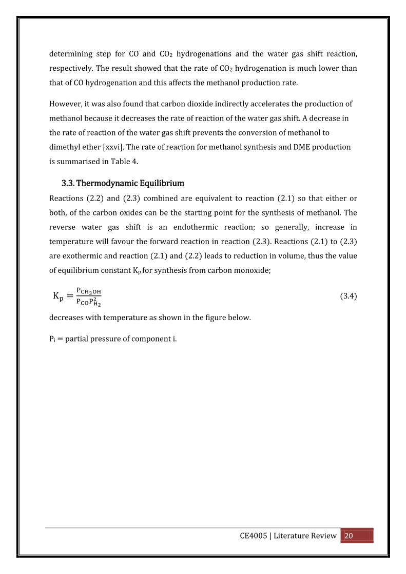
3.3. Thermodynamic Equilibrium
Reactions (2.2) and (2.3) combined are equivalent to reaction (2.1) so that either or
both, of the carbon oxides can be the starting point for the synthesis of methanol. The
reverse water gas shift is an endothermic reaction; so generally, increase in
temperature will favour the forward reaction in reaction (2.3). Reactions (2.1) to (2.3)
are exothermic and reaction (2.1) and (2.2) leads to reduction in volume, thus the value
of equilibrium constant Kp for synthesis from carbon monoxide;
(3.4)
decreases with temperature as shown in the figure below.
Pi = partial pressure of component i.
CE4005 | Literature Review 21
Figure 9. Thermodynamics of methanol synthesis. Variation of equilibrium constant kp with temperature and pressure
[iv]
Increase in the value of equilibrium constant with pressure is due to non-ideality. Thus
if the catalyst is sufficiently active, high conversion of methanol will be obtained at high
pressures and low temperatures. The use of high pressure commercially is expensive
both of capital and gas compression. Therefore, with a very active catalyst, it is most
economical to use lower pressure and obtain the same conversions as at high pressures
but at lower temperatures. Figure 9 shows a variation of equilibrium constant with
temperature and pressures. It shows that a catalyst which is only active at 350°C or
above such as the ZnO/Cr catalyst will require an operating pressure of 300 bar to
achieve a conversion to methanol of 3% while a more active catalyst such as the
Cu/ZnO/Al2O3 catalyst will obtain the same conversion at 50 bar [iv].
Thermodynamic equilibrium limits the maximum yields of carbon oxides to methanol.
Due to the strongly non ideal behaviour of gases at conditions used commercially,
equilibrium equations necessarily involve fugacity. The equilibrium composition of any
CE4005 | Literature Review 22
mixture of carbon oxides, water, methanol, hydrogen and inert can be calculated using
the equations below. These equations corresponds to reactions in equation 3.1 and 3.3.
Kf1 = fCH3OH/fCOfH2 (3.5)
Kf2 = fCO2fH2/fCOfH2O (3.6)
Where fi is the fugacity of component i in atmospheres [ii].
3.4. Selectivity
Carbon monoxide and carbon dioxide can also react with hydrogen to produce by-
products such as ethers, hydrocarbons and higher alcohols.
CO +3H2 CH4 +H2O (ΔH298K = -206.17kJ/mol, ΔG°= -142.25kJ/mol)
(3.7)
2CO +4H2 CH3OCH3 +H2O (ΔH298K = -204.82kJ/mol, ΔG°= -67.20kJ/mol)
(3.8)
2CO +4H2 C2H5OH +H2O (ΔH298K = -2 . 8kJ/mol, ΔG°= -122.55kJ/mol)
(3.9)
These reactions (equation 3.7-3.9) are more exothermic than the methanol synthesis
reactions and their formation involves larger negative change of free energy. Methanol
is thermodynamically less stable and less likely to be formed from carbon monoxide and
hydrogen than the other possible products such as methane. Kinetic factors are used to
determine the product formed. A selective catalyst is used to favour a reaction path
leading to the desired product (methanol) with a minimum of by-products [iv].
CE4005 | Literature Review 23
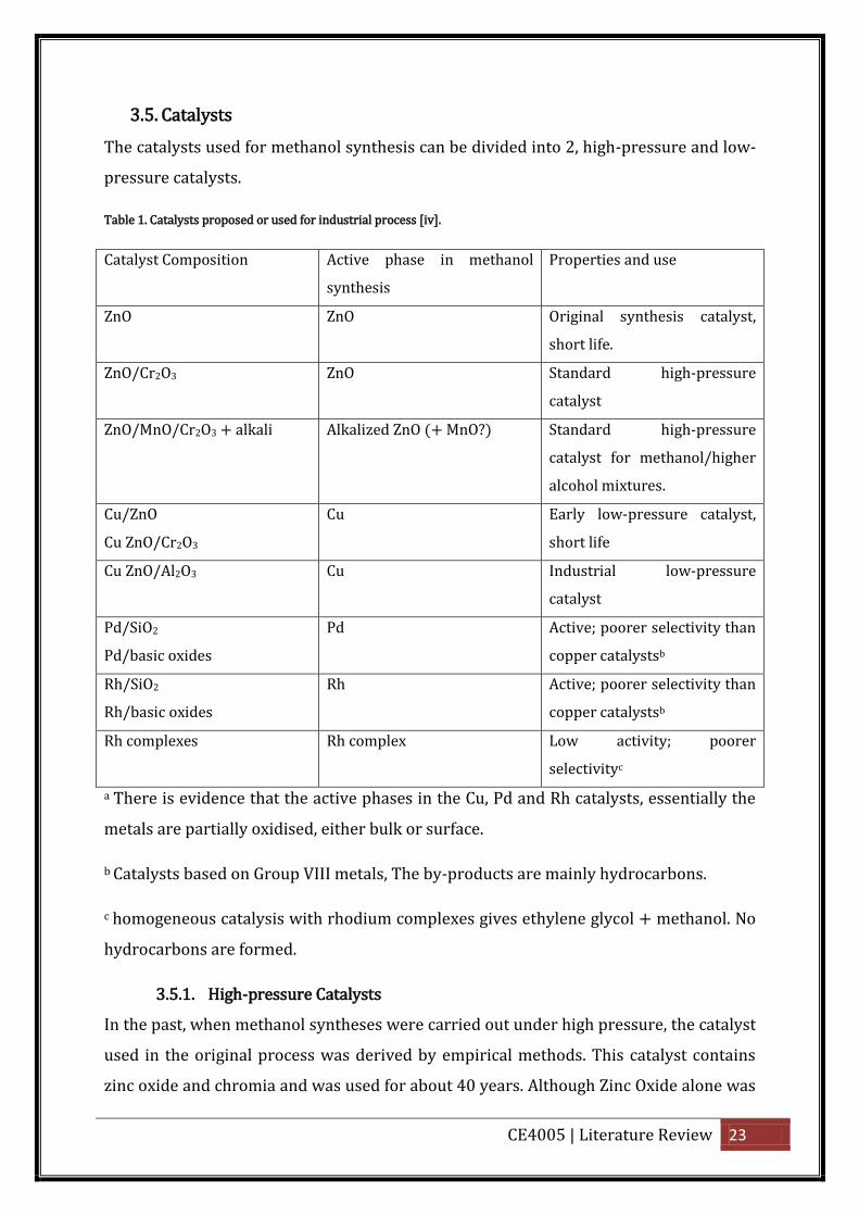
3.5. Catalysts
The catalysts used for methanol synthesis can be divided into 2, high-pressure and low-
pressure catalysts.
Table 1. Catalysts proposed or used for industrial process [iv].
Catalyst Composition Active phase in methanol
synthesis
Properties and use
ZnO ZnO Original synthesis catalyst,
short life.
ZnO/Cr2O3 ZnO Standard high-pressure
catalyst
ZnO/MnO/Cr2O3 + alkali Alkalized ZnO (+ MnO?) Standard high-pressure
catalyst for methanol/higher
alcohol mixtures.
Cu/ZnO
Cu ZnO/Cr2O3
Cu Early low-pressure catalyst,
short life
Cu ZnO/Al2O3 Cu Industrial low-pressure
catalyst
Pd/SiO2
Pd/basic oxides
Pd Active; poorer selectivity than
copper catalystsb
Rh/SiO2
Rh/basic oxides
Rh Active; poorer selectivity than
copper catalystsb
Rh complexes Rh complex Low activity; poorer
selectivityc
a There is evidence that the active phases in the Cu, Pd and Rh catalysts, essentially the
metals are partially oxidised, either bulk or surface.
b Catalysts based on Group VIII metals, The by-products are mainly hydrocarbons.
c homogeneous catalysis with rhodium complexes gives ethylene glycol + methanol. No
hydrocarbons are formed.
3.5.1. High-pressure Catalysts
In the past, when methanol syntheses were carried out under high pressure, the catalyst
used in the original process was derived by empirical methods. This catalyst contains
zinc oxide and chromia and was used for about 40 years. Although Zinc Oxide alone was
CE4005 | Literature Review 24
a good catalyst for methanol synthesis at high temperature and temperatures above
350°C, it was not stable and it quickly lost it activities which means it has to be replaced
frequently. Through research, it was found that chromia acts as a stabilizer for zinc
oxide by preventing the growth of the zinc oxide crystals and by so doing preventing die
off. The Zinc oxide/chromia catalyst was tolerant of the impure synthesis gas and could
have a plant life of several of years. This catalyst was not very selective and depending
on synthesis conditions as much as 2% of the inlet carbon oxides could be converted to
methane and a similar proportion to dimethyl ether. The very exothermic nature of the
side reaction calls for a careful control of catalyst temperature [iv].
3.5.2. Low-pressure Catalysts
The low-pressure process is based on high activity catalysts. Copper oxide was found to
be very effective for methanol synthesis when added to zinc oxide. The zinc
oxide/chromia catalysts also showed increase in activity when Copper oxide was added
to it, so it could be used at temperatures as low as 300°C. However catalysts containing
copper were not stable and lost activity e.g. a Zn/Cu/Cr catalyst in atomic proportions
of 6: 3 : 1 lost 40% of its activity in 72 hours. The work of ICI on methanol synthesis
resulted in the production of more stable copper catalysts. In the modern copper/zinc
oxide/alumina synthesis catalysts, high activity and stability are obtained by optimizing
the composition and producing very small particles of the mixture in a very intimate
mixture precipitated at controlled pH in which the acidic and alkaline solutions are
mixed continuously. Catalysts made by the continuous process were used in the first
(1966) low-pressure methanol synthesis plants operating at 50 bar and they had lives
of more than 3 years as well as producing methanol of a higher purity than the high-
pressure process. Further development resulted in catalysts suitable for operation at
100 bar, around the optimum operating pressure for plants capable of producing 1000
tonnes per day of methanol. Zinc oxide/alumina is not sufficiently refractory as a
support at 100 bar, but a more refractory support is provided by using some of the zinc
component as a compound with the alumina component; as zinc spinel (ZnO.Al2O3),
which is produced in a finely divided state.
In recent years, some new catalysts and process configuration has been proposed.
Although not yet commercially viable, some aspects may form the basis of methanol
synthesis in the future. Two novel supported catalysts have been reported. ‘Raney
CE4005 | Literature Review 25
copper’ prepared by leaching ternary copper/zinc/aluminium alloys with strong
aqueous sodium hydroxide and ‘extremely active thorium compounds’. Future
developments of the conventional process are likely to be mainly capital savings and
improvements in energy efficiency. Catalysts of improved performance will doubtless
enable process designers to overcome chemical engineering constraints [iv].
CE4005 | Literature Review 26
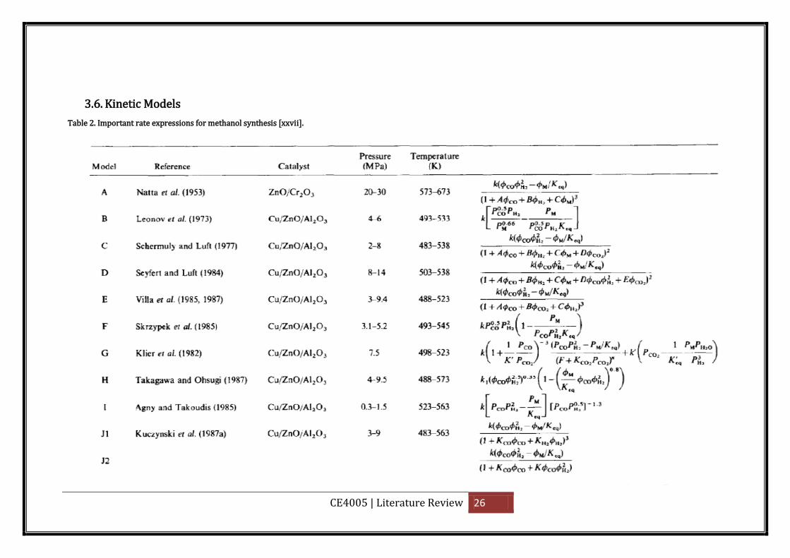
3.6. Kinetic Models
Table 2. Important rate expressions for methanol synthesis [xxvii].
CE4005 | Literature Review 27
3.6.1. Natta et al (1953)
One of the earliest most influential works on methanol synthesis was that of Natta et al.
[xxviii]. His studies included measurements of the effects of composition, temperature
and pressure on methanol synthesis reaction rates. The kinetics of methanol synthesis
was studied in a continuous operating apparatus at temperatures between 300 and
400°C, pressure between 150 and 300atm and at different CO/H2 ratios in the feed
gases.
The surface reaction between one chemiadsorbed molecule of carbon monoxide and
two hydrogen molecules to produce one molecule of methanol chemiadsorbed on the
solid catalyst is the slowest intermediate step which controls the whole rate of reaction.
Natta’s wo k ep esents one of the widest anges of conditions in all published
methanol literature. Natta assumed that the rate-determining step was the trimolecular
reaction of carbon monoxide and hydrogen on the surface of the catalyst. From
experimental data, he expressed the correlation between reaction rate, fugacity of
components, and some constants (mainly depending upon the adsorption equilibrium
constants). That led to the correlation in equation (3.10) below.
/
( (3.10)
Where: r = rate of reaction, f = fugacity, Keq = equilibrium constant and A,B,C and D are
adsorption rate constants.
The established correlation allows calculating the quantity of methanol produced, as a
function of temperature, space velocity, and composition of feed gas [xxviii].
3.6.2. Rozovskii (1980) and Klier (1982)
Since Natta’s esea ch, catalysts have been imp oved continuously, esulting in
methanol synthesis plants that operate at lower pressures and temperatures. In recent
time, much kinetics have been proposed but unfortunately, difference in operating
conditions, catalyst used and feed gas composition has made it difficult to arrive at a
final conclusion on the kinetics and reaction mechanism.
The pioneering work by Natta has been expanded and improved by many other
researchers. Klier et al., [xxix] assumed that a small amount of carbon dioxide is
CE4005 | Literature Review 28
hydrogenated directly to methanol and the remaining carbon dioxide competes for
active sites on the surface of the catalyst with other reactants. They attempted to
formulate a mechanism and rate law encompassing all surface phenomena. The rate law
formulated based on those assumptions is given below:
/
(
k (p
) (3.11)
Where:
A is the rate constant,
pi is partial pressure of component i in atmospheres,
Keq is equilibrium constant for CO,
’eq is equilibrium constant for CO2,
kCO , kH2 , kCO2 are desorption and adsorption parameters.
This model is consistent with all the physical characteristics of the CuZnO catalysts and
supports earlier findings that an intermediate oxidation state of the catalyst is its active
state.
Based on the stoichiometry of equation (2.2), Rozovskii [xxx] contends that methanol
forms only via carbon dioxide hydrogenation and proposed the rate equation below:
(3.12)
According to Rozovskii’s mechanism, carbon dioxide also participates in the reverse
water-gas shift reaction as shown in equation (2.3) with the rate equation given below:
(3.13)
Values of rate constants A-D are still undetermined [xxx].
3.6.3. Agny and Takoudis (1985)
Using a U shaped fixed bed reactor and a CuO/ZnO/Al2O3 catalyst operated at a
pressure between 0.3 to 1.5Mpa and temperature between 523-563K, Agny and
Takoudis [xviii] made use of the Langmuir-Hinshelwood kinetic model, they proposed
CE4005 | Literature Review 29
that that the adsorbed CO molecule dissociatively adsorbs a hydrogen molecule to form
the formyl intermediate CHO- with H2/CO ratio of 0.5/1 which is present in the
( . term of the kinetic equation they came up with equation 3.14 below. n was
determined as -1.3 empirically.
k (P P
(P P
. (3.14)
Where:
K is reaction rate constant = 0.991*10-2 exp (-18330/RT)
Keq is the thermodynamic equilibrium constant of carbon monoxide
hydrogenation reaction (equation 2.1)
Pi is the partial pressure of component i in atmosphere,
n is empirical constant = 1.3 ± 0.03.
The CH-O intermediate was postulated to be the abundant surface intermediate. The
rate determining step was the surface reaction between the adsorbed hydrogen and
methoxy intermediate CH3O-. They also suggested that trace amount of carbon dioxide
detected at the reactor effluent stream was produced from the water gas shift reaction
(equation 3.3) and the redox reaction from the oxidised state to the reduced state of the
catalyst. A carbon dioxide free synthesis gas was used as feed; therefore no term
corresponding to carbon dioxide was incorporated in the rate equation.
The value of the pre-exponential factor and the overall activation energy at 523k are
13600 mol/(s atm gcat) and 34000 cal/gmol respectively [xviii].
3.6.4. Skrzypek's (1985 and 1991)
Skrzypek et.al (1985) [ xxxi ] carried out the Analysis of the low-temperature methanol
synthesis in a single commercial isothermal Cu-Zn-Al catalyst pellet using the dusty-gas
diffusion model. They came up with a rate equation of
kp . P
(1
) (3.15)
CE4005 | Literature Review 30
Where:
r is the rate of reaction,
k is the reaction rate constant = 0.830 exp (-23750/RT)
(3.16),
pi is partial pressure of component i in atmosphere and
keq = thermodynamic equilibrium constant.
In 1991, they further investigated the kinetics of methanol synthesis over commercial
copper/zinc oxide/alumina catalysts at a temperature between 187-277°C and pressure
between 30-90 bar. A wide range of parameters was applied, especially that of the inlet
concentrations of reactant. They concluded that methanol synthesis occurs from CO2
rather than from CO and that the basic reactions are:
CO2+3H2⇄CH3OH+H2O and CO2+H2⇄CO+H2O (3.17)
They also demonstrated experimentally that methanol cannot be formed from hydrogen
and carbon monoxide without the presence of water.
Langmuir-Hinshelwood mechanism where CO2 and H2 react on the surface with few
intermediate steps was used. The rate determining step came out to be
CO2* + H2 * ⇄ H2CO2* (3.18)
(* denotes adsorbed species). The resulting rate equations this time around based on
equation 2.2 and 2.3 are:
( (
)(
))
(3.19)
( (
)( ))
(3.20)
den 1 p p p p p (3.21)
This kinetic model is based on measurements on a deactivated catalyst, and the effect of
deactivation is not accounted for. Hence, the reaction rates are probably too slow [xxxi].
CE4005 | Literature Review 31
3.6.5. Lim (2009)
The theory by Klier et.al (1982) that copper is reduced or oxidised by the adsorption of
CO and CO2, suggests that there are different adsorption sites for CO and CO2. Analysing
published reports shows that there are conflicting viewpoints on the identity of the
active sites on Cu containing catalysts for the methanol synthesis. In most published
reports, CO hydrogenation (Equation 2.1) has been considered to be the most
significant reaction for methanol production. A possible reason for the difference in
results is that CO2 hydrogenation also occurs to some extent under certain reaction
conditions. To solve this problem, Lim et al., took into account the hydrogenation of
both CO and CO2 and studied the kinetics of methanol synthesis over
Cu/ZnO/Al2O3/ZrO2 catalyst that was developed and selected to evaluate the effect of
carbon dioxide on the reaction rates due to its high activity and stability.
A kinetic mechanism where CO and CO2 are assumed to adsorb on different sites of Cu
was suggested for the development of hydrogenation reaction rates, while hydrogen is
supposed to be adsorbed on the site of ZnO. Since each overall reaction is made up of
several elementary steps, they developed various rate determining steps and estimated
to find the best fit model for methanol synthesis by using experimental data. The
experimental data in their study suggested the augmentation of additional reactions
other than the three main reactions (Equation 2.1, 2.2 and 2.3).
The resulting rate equations from this study is given below.
Where : ln .
29.07 (3.26)
ln .
5.639 (3.27)
KPC = KPA * KPB (3.28)
(3.22)
(3.23)
(3.24)
(3.25)
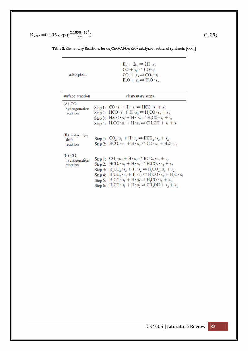
CE4005 | Literature Review 32
KDME =0.106 exp ( .
(3.29)
Table 3. Elementary Reactions for Cu/ZnO/Al2O3/ZrO2 catalysed methanol synthesis [xxxii]

CE4005 | Literature Review 33
Table 4. Reaction rates for methanol synthesis reaction and DME production [xxvi].
CE4005 | Literature Review 34
3.6.6. Literature Review Conclusion
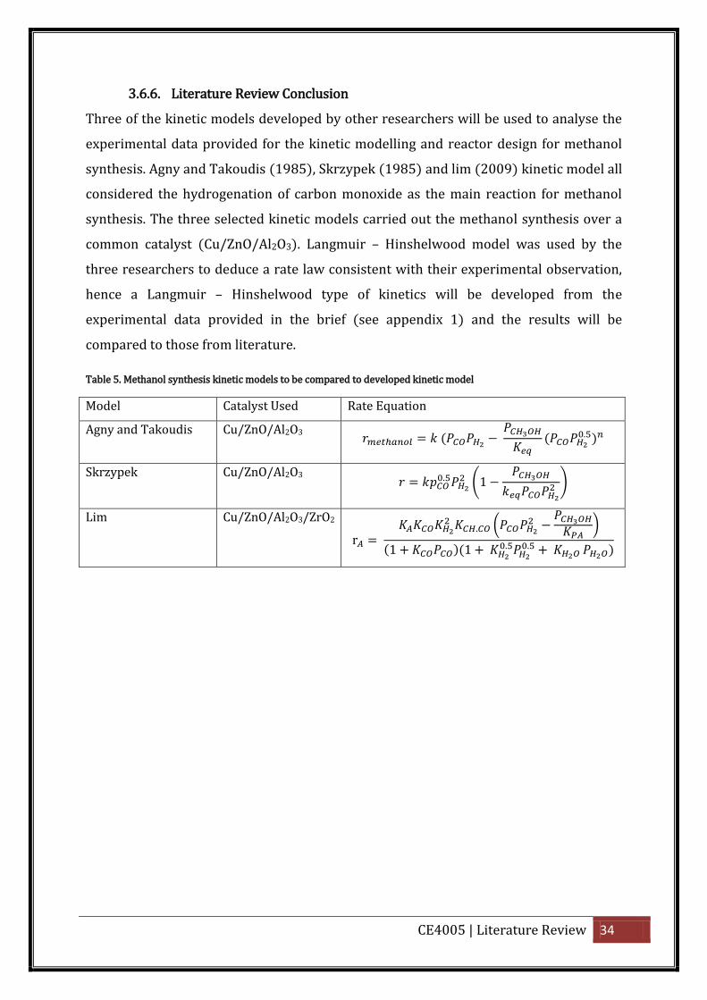
Three of the kinetic models developed by other researchers will be used to analyse the
experimental data provided for the kinetic modelling and reactor design for methanol
synthesis. Agny and Takoudis (1985), Skrzypek (1985) and lim (2009) kinetic model all
considered the hydrogenation of carbon monoxide as the main reaction for methanol
synthesis. The three selected kinetic models carried out the methanol synthesis over a
common catalyst (Cu/ZnO/Al2O3). Langmuir – Hinshelwood model was used by the
three researchers to deduce a rate law consistent with their experimental observation,
hence a Langmuir – Hinshelwood type of kinetics will be developed from the
experimental data provided in the brief (see appendix 1) and the results will be
compared to those from literature.
Table 5. Methanol synthesis kinetic models to be compared to developed kinetic model
Model Catalyst Used Rate Equation
Agny and Takoudis Cu/ZnO/Al2O3 (
(
.
Skrzypek Cu/ZnO/Al2O3
. (1
)
Lim Cu/ZnO/Al2O3/ZrO2
. (
)
(1 (1 .
.
CE4005 | Work Plan and Methodology 35
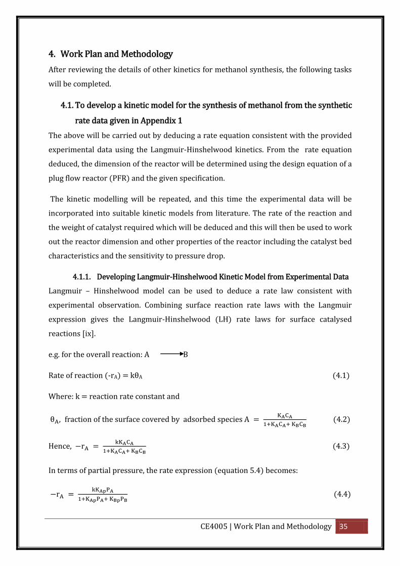
4. Work Plan and Methodology
After reviewing the details of other kinetics for methanol synthesis, the following tasks
will be completed.
4.1. To develop a kinetic model for the synthesis of methanol from the synthetic
rate data given in Appendix 1
The above will be carried out by deducing a rate equation consistent with the provided
experimental data using the Langmuir-Hinshelwood kinetics. From the rate equation
deduced, the dimension of the reactor will be determined using the design equation of a
plug flow reactor (PFR) and the given specification.
The kinetic modelling will be repeated, and this time the experimental data will be
incorporated into suitable kinetic models from literature. The rate of the reaction and
the weight of catalyst required which will be deduced and this will then be used to work
out the reactor dimension and other properties of the reactor including the catalyst bed
characteristics and the sensitivity to pressure drop.
4.1.1. Developing Langmuir-Hinshelwood Kinetic Model from Experimental Data
Langmuir – Hinshelwood model can be used to deduce a rate law consistent with
experimental observation. Combining surface reaction rate laws with the Langmuir
expression gives the Langmuir-Hinshelwood (LH) rate laws for surface catalysed
reactions [ix].
e.g. for the overall reaction: A B
Rate of reaction (-rA) = kθA (4.1)
Where: k = reaction rate constant and
θ , f action of the su face cove ed by adso bed species
(4.2)
Hence,
(4.3)
In terms of partial pressure, the rate expression (equation 5.4) becomes:
(4.4)
CE4005 | Work Plan and Methodology 36
Where
(4.5)
ka is adsorption rate constant,
kd is desorption rate constant,
pi is partial pressure of component i ,
CA is gas composition of component A,
CB is gas composition of component B.
The following assumptions will be used to deduce rate law consistent with the
experimental data provided.
1. Surface reaction is first order.
2. Reaction is essentially irreversible.
Conclusion can be drawn from the rate of disappearance of H2, on the partial
pressure of hydrogen, carbon monoxide and methanol.
Analyse the experimental data to find dependence on the product methanol.
Analyse the experimental data to find dependence on carbon monoxide.
Analyse the experimental data to find dependence on hydrogen.
Deduce Langmuir-Hinshelwood type rate equation from the analysis above.
Find the kinetic parameters, k and K values.
4.1.2. Experimental Data Incorporated into Kinetic Model From Literature
Sample Model: Agny and Takoudis Kinetic Model
k (P P
(P P
. (4.6)
k = 0.991*10-2 exp (-18330/RT). (4.7)
Log10Keq = (3921/T) – 7.971 log10T + 0.002499 T – (2.953*10-7)T2 + 10.2
(dimensionless). (4.8)
rmethanol is rate of reaction,
k is reaction rate constant ,
Pi is the partial pressure of component i (atmosphere),
n is the empirical constant,

CE4005 | Work Plan and Methodology 37
Keq is the thermodynamic equilibrium constant and
T is temperature.
For Adiabatic PFR , the energy balance can be written as:
[(
] (4.9)
For nonadiabatic PFR, the energy balance can be written as:
[(
] (4.10)
The design equation of a FBCR,
∫
(
(4.11)
Where:
Tad is adiabatic temperature rise,
T is reaction temperature,
TO is reactor inlet temperature,
Ts is surrounding temperature/temperature of coolant,
ΔHreaction = Heat of reaction
FA0 is molar flow,
is specific mass flow rate,
CP is specific heat of the system.
W is weight of catalyst,
XA is fractional conversion and
-rA is the rate of reaction.
The weight of the catalyst calculated by simultaneous numerical solution of the material
and energy balance will be used to calculate the reactor dimension by following the
steps below:
1. Choose a value of conversion, X.
2. Depending on the desired reactor set up, calculate T from equation 4.9 for adiabatic
and 4.10 for non-adiabatic.
CE4005 | Work Plan and Methodology 38
3. Calculate the kinetic parameters k and Keq from equation 4.6 and 4.7. (Other kinetic
model will have different kinetic parameters).
4. Substitute the partial pressure, Pi values into the kinetic model rate equation
5. Calculate –rA (rate of reaction) using the kinetic model rate equation
6. Calculate
( (4.12)
7. Repeat step (1) to (6) for values of conversion X between 0 and 0.9
8. Calculate ∑ (4.13)
Where G* is the average of two successive values of G and is the increment.
9. Plot the results with temperature on the y-axis and conversion on the x-axis.

CE4005 | Work Plan and Methodology 39
4.2. Simulating a Plant-Scale Catalytic Reactor
Using the kinetic model result obtained from section 4.1, the dimension of a catalytic
scale reactor will be determined.
Find FAo , CAo and which a e some of the values needed to find the eacto
dimension.
From the material balance, FAo = voCAo (4.14)
Space velocity = 10000m3/hr/m3 of reactor volume
Space velocity =
=
hence, =
(4.15)
= 10000m3/hr , = 1 * 10-4
V = 1m3
v =
v = 10000
2.78
PV = nRT (4.16)
P n
P = ΣPi (4.17)
and
= CAo (4.18)
Hence, CAo =
(4.19)
Composition: 70 mol% H2; 30 mol% CO; r.m.m H2 = 2 , CO = 28
[(mola composition (H2) * r.m.m (H2) * FAo)+( molar composition of CO * r.m.m of
CO * FAo)]/1000 (4.20)
where:
FAo is molar flow at reactor inlet,
CE4005 | Work Plan and Methodology 40
vo is volumetric flow rate,
CAo is initial concentration; is residence time,
is specific mass flow ate; P is pressure,
Pi is partial pressure of component i; n is number of moles,
V is reactor volume,
R is molar gas constant and
T is temperature.
4.2.1. Reactor Volume
For the shell and tube reactor, assuming the catalyst bed occupies 1/3 of the reactor
volume i.e. 1/3VReactor = VCatalyst, i.e. the catalyst will occupy a third of the reactor
volume. Another third of the reactor volume will be occupied by the shell space and the
final third will be occupied by the space between the catalyst bed and the top and
bottom dome heads. This assumption will help to calculate the dimension of reactor
needed without too much complication.
The volume of the reactor will be determined from the catalyst weight using the
equation: VC = WC/ρC = 1/3VReactor (4.21)
Where:
VC is the volume of catalyst
WC is weight of catalyst,
ρC is the bulk density of catalyst,
VReactor is the volume of cylindrical section of reactor
om the volume, the eacto length, diamete and the catalyst bed’s cha acte istics can
be determined.
The total volume of reactor is the volume of cylindrical section + volume of dome
closures.
4.2.2. Reactor Length and Diameter
For a cylindrical vessel, the relationship between the length and the volume of a
cylinder is given as: VR =
(4.22)
CE4005 | Work Plan and Methodology 41
Where:
VR = volume of the reactor
D = diameter of reactor
= length of reactor
(Note: The reactor volume does not include the volume occupied by the dome head
closures).
Total length of reactor = length of cylindrical section + length of hemispherical head
closure
Assumption
Assuming a diameter to length ratio (D : ) of 1:4
Hence: 4 (4.23)
The volume of the reactor can be rewritten as:
VR =
4 (4.24)
VR πD3 (4.25)
Rearrange to get D
D = √
(4.26)
4.2.3. Reactor Dome Closure
The reactor is cylindrical and there are four principal types of ends used for a cylindrical
vessel.
1. Torispherical heads.
2. Hemispherical heads.
3. Ellipsoidal heads.
4. Flat plates and formed flat heads.
CE4005 | Work Plan and Methodology 42
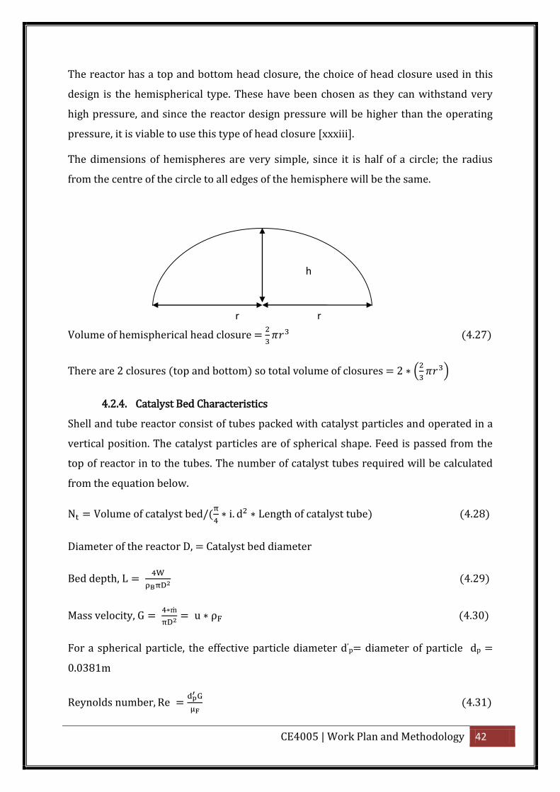
The reactor has a top and bottom head closure, the choice of head closure used in this
design is the hemispherical type. These have been chosen as they can withstand very
high pressure, and since the reactor design pressure will be higher than the operating
pressure, it is viable to use this type of head closure [xxxiii].
The dimensions of hemispheres are very simple, since it is half of a circle; the radius
from the centre of the circle to all edges of the hemisphere will be the same.
Volume of hemispherical head closure =
(4.27)
There are 2 closures (top and bottom) so total volume of closures = 2 (
)
4.2.4. Catalyst Bed Characteristics
Shell and tube reactor consist of tubes packed with catalyst particles and operated in a
vertical position. The catalyst particles are of spherical shape. Feed is passed from the
top of reactor in to the tubes. The number of catalyst tubes required will be calculated
from the equation below.
N olume of catalyst bed/(
i. d Length of catalyst tube (4.28)
Diameter of the reactor D, = Catalyst bed diameter
Bed depth, L
(4.29)
Mass velocity, G
u ρ (4.30)
For a spherical particle, the effective particle diameter d’p= diameter of particle dp =
0.0381m
eynolds numbe , e
(4.31)
r r
h
CE4005 | Effect of Coolant Temperature 43
Pressure drop ( P
(4.32)
Friction factor, f [1.7 (
] (
(4.33)
Fluid density ρ (
)
(4.34)
Superficial linear velocity, u
(4.35)
4.3. Sensitivity to pressure drop
Calculate pressure drop, from equation 4.32
Choose values of around that calculated in the step above.
Calculate the bed depth, L for the selected from equation 4.17
Rearrange equation 4.20 to give (
(4.36)
Calculate the diameter from
√
(4.37)
Tabulate the result
Plot a graph of on the y-axis, Diameter and bed depth on the x-axis
Observe the trend in D and L as pressure drop increase or drop.
Draw a conclusion on the trend above.
4.4. Effect of Coolant Temperature
Due to the exothermic nature of the methanol synthesis reaction (CO + 2H2 CH3OH
ΔH298K = -90.64kJ/mol) there is a need to take out the heat of the reaction. Cooling
water can be used to take out the heat of the reaction. The temperature of the cooling
water required can be found graphically by following the steps below.
Find the equilibrium conversion, Xe from the equation:
(
( (4.38)
Where Ke is the thermodynamic equilibrium constant and T is the equilibrium
temperature.
CE4005 | Results and Discussion 44
Plot a graph of equilibrium conversion Xe and conversion X on the y-axis against
temperature, T on the x-axis.
The intersection of the equilibrium conversion as a function of temperature with
temperature-conversion relationships suggests a reasonable coolant
temperature for the shell side in order to achieve the equilibrium conversion.
4.5. Modelling with ASPEN Process Modelling Software.
ASPEN, process simulation software will be used to model the methanol synthesis
process. The reactor will be modelled as an adiabatic plug flow reactor. The reactor is
big and therefore will approach adiabatic regime without the need for special insulation
due to negligible heat loss. Rate of chemical reaction also governs this. The faster the
rate of the chemical reaction, the easier it is to obtain adiabatic regime.
The adiabatic reactor can be controlled by the inlet composition of the reaction mixture
and the inlet temperature (473K). The composition of the inlet mixture for the
methanol synthesis given in the specification sheet is 70mol% H2; 30mol% CO.
A kinetic model will be selected and modelled on ASPEN using the data for kinetic
analysis provided. The composition and the reactor inlet temperature will be varied in
order to test the performance of the reactor. A sensitivity analysis will also be carried
out to check the effect of feed temperature on methanol production.
4.6. Gantt Chart
An academic supervisor will monitor the progress of this project. A Gantt chart will be
used to monitor and control the progress of this project against the schedule. Time
management is important in order to provide a project that will be of good quality and
that will be delivered on time. A Gantt chart containing the project schedule has been
attached to appendix 5.
5. Results and Discussion
5.1. Developing a kinetic model from experimental data
From the experimental data provided in Table 6 below, a kinetic model will be
developed for methanol synthesis. “ he data we e gene ated fo the ove all eaction as
it would occur in a back mixed, gradient less, experimental reactor at realistic reaction
CE4005 | Results and Discussion 45
conditions. The final data set is from a statistically designed, central composite set of
simulated experiments, to which 5% random error was added. It comprises a total of 27
simulated esults”[xxxiv].
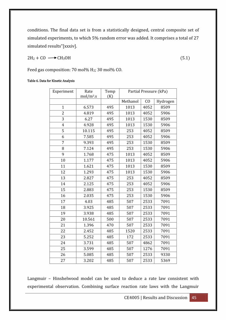
2H2 + CO CH3OH (5.1)
Feed gas composition: 70 mol% H2; 30 mol% CO.
Table 6. Data for Kinetic Analysis
Experiment Rate mol/m3.s
Temp (K)
Partial Pressure (kPa)
Methanol CO Hydrogen
1 6.573 495 1013 4052 8509
2 4.819 495 1013 4052 5906
3 6.27 495 1013 1530 8509
4 4.928 495 1013 1530 5906
5 10.115 495 253 4052 8509
6 7.585 495 253 4052 5906
7 9.393 495 253 1530 8509
8 7.124 495 253 1530 5906
9 1.768 475 1013 4052 8509
10 1.177 475 1013 4052 5906
11 1.621 475 1013 1530 8509
12 1.293 475 1013 1530 5906
13 2.827 475 253 4052 8509
14 2.125 475 253 4052 5906
15 2.883 475 253 1530 8509
16 2.035 475 253 1530 5906
17 4.03 485 507 2533 7091
18 3.925 485 507 2533 7091
19 3.938 485 507 2533 7091
20 10.561 500 507 2533 7091
21 1.396 470 507 2533 7091
22 2.452 485 1520 2533 7091
23 5.252 485 172 2533 7091
24 3.731 485 507 4862 7091
25 3.599 485 507 1276 7091
26 5.085 485 507 2533 9330
27 3.202 485 507 2533 5369
Langmuir – Hinshelwood model can be used to deduce a rate law consistent with
experimental observation. Combining surface reaction rate laws with the Langmuir
CE4005 | Results and Discussion 46
expression gives the Langmuir-Hinshelwood (LH) rate laws for surface catalysed
reactions [ix].
The following assumptions will be used to deduce rate law consistent with the
experimental data provided in Table 6 above.
Surface reaction is first order
Reaction can be assumed to be essentially irreversible
Conclusion can be drawn from the rate of disappearance of H2, on the partial
pressure of hydrogen carbon monoxide and methanol.
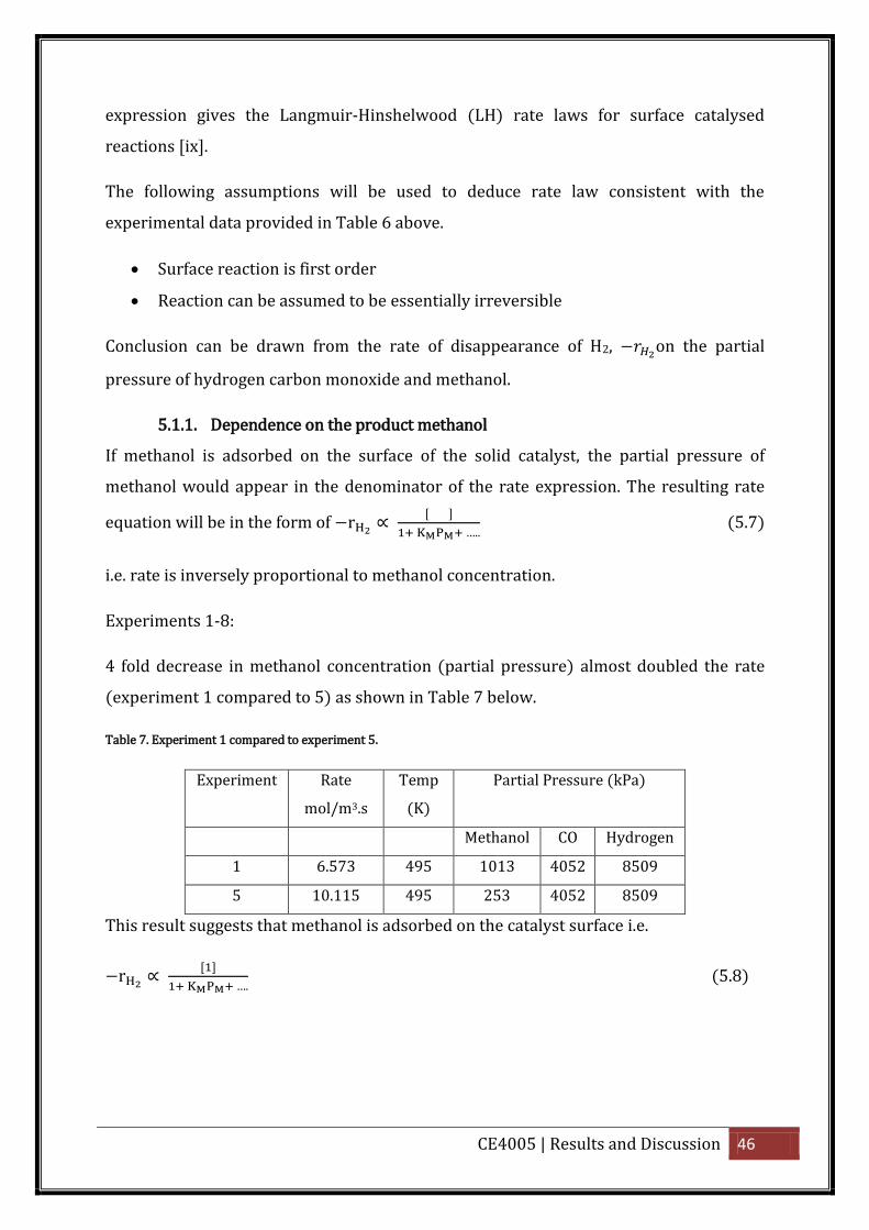
5.1.1. Dependence on the product methanol
If methanol is adsorbed on the surface of the solid catalyst, the partial pressure of
methanol would appear in the denominator of the rate expression. The resulting rate
equation will be in the form of [
.. (5.7)
i.e. rate is inversely proportional to methanol concentration.
Experiments 1-8:
4 fold decrease in methanol concentration (partial pressure) almost doubled the rate
(experiment 1 compared to 5) as shown in Table 7 below.
Table 7. Experiment 1 compared to experiment 5.
Experiment Rate
mol/m3.s
Temp
(K)
Partial Pressure (kPa)
Methanol CO Hydrogen
1 6.573 495 1013 4052 8509
5 10.115 495 253 4052 8509
This result suggests that methanol is adsorbed on the catalyst surface i.e.
[
. (5.8)

CE4005 | Results and Discussion 47
5.1.2. Dependence on Carbon Monoxide
Table 8. Experiments to deduce the dependence on carbon monoxide
Experiment Rate
mol/m3.s
Temp
(K)
Partial Pressure (kPa)
Methanol CO Hydrogen
1 6.573 495 1013 4052 8509
3 6.27 495 1013 1530 8509
5 10.115 495 253 4052 8509
7 9.393 495 253 1530 8509
Experiments 1 and 3, 5 and 7, 9 and 11 shows that almost 3 folds increase in the partial
pressure of carbon monoxide has little effect on the rate of the reaction. This suggests
that carbon monoxide is very weakly adsorbed or goes directly into gas phase.
i.e. 1 (5.9)
5.1.3. Dependence on Hydrogen
Experiments 1 and 2, 3 and 4, 5 & 6, 7 & 8, 9 & 10, 13 & 14, 15 & 16 shows that rate
decrease with decrease in the partial pressure of hydrogen when the partial pressure of
methanol and carbon monoxide is kept constant as shown on Table 9 below.
Table 9. Effect of decreasing the partial pressure of hydrogen on the rate of reaction.
Experiment Rate
mol/m3.s
Temp
(K)
Partial Pressure (kPa)
Methanol CO Hydrogen
1 6.573 495 1013 4052 8509
2 4.819 495 1013 4052 5906
This suggests that hydrogen is strongly adsorbed on the catalyst surface, hence
[
. (5.10)
Combining equations 5.8, 5.9 and 5.10 suggests that the rate law is of the form:
[
(5.11)
Equation 5.11 can be rewritten as:
CE4005 | Results and Discussion 48
[
whe e
(5.12)
Where:
is ate of disappea ance of hyd ogen ate of fo mation of methanol,
k is the methanol synthesis rate constant,
Pi is partial pressure of component i,
KM is methanol adsorption equilibrium constant and
is hydrogen adsorption equilibrium constant.
5.1.4. Finding k and K Values
The rate law deduced from the experimental data provided (equation 5.12) is given
below:
To evaluate the reaction rate constant, k and the rate law parameters and
Rearrange equation 5.12.
(5.13)
This can be re-written as:
(5.14)
(Equation of a straight line) (5.15)
Appropriate data points will be selected from the experimental data available on Table
6 to plot a graph of y against x
Where:
y
, P /P (5.16)
c
(5.17)
CE4005 | Results and Discussion 49
m
/
(5.18)
Since the reaction rate constant and adsorption parameters, Ki are functions of
temperature, they should be found at constant temperature.
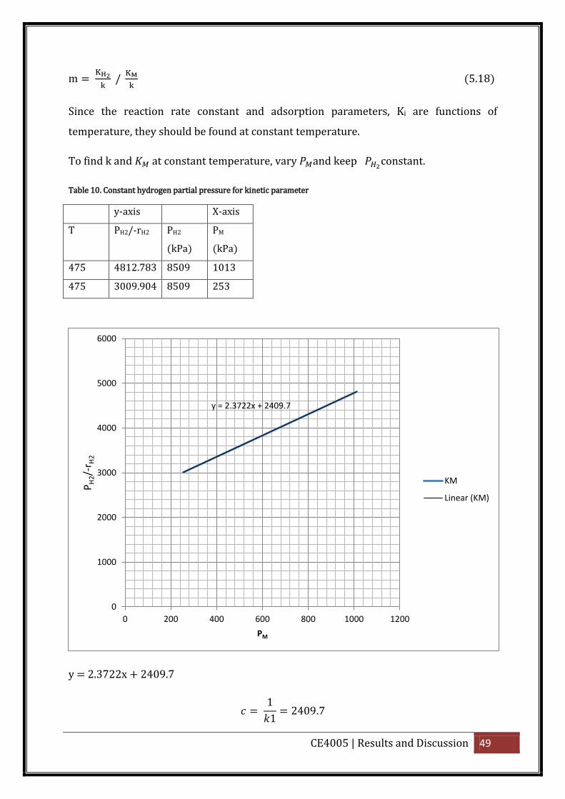
To find k and at constant temperature, vary and keep constant.
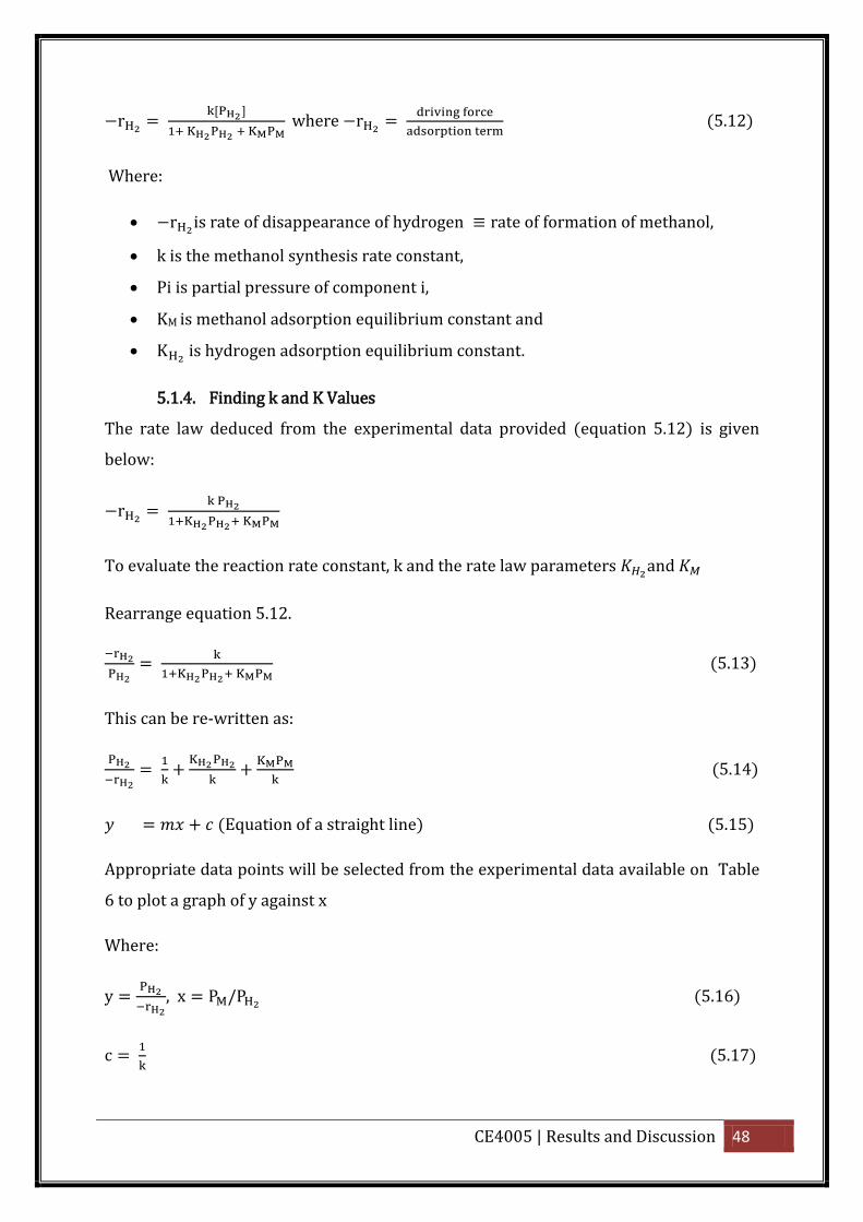
Table 10. Constant hydrogen partial pressure for kinetic parameter
y-axis X-axis
T PH2/-rH2 PH2
(kPa)
PM
(kPa)
475 4812.783 8509 1013
475 3009.904 8509 253
y = 2.3722x + 2409.7
1
1 2409.7
y = 2.3722x + 2409.7
0
1000
2000
3000
4000
5000
6000
0 200 400 600 800 1000 1200
PH
2/-
r H2
PM
KM
Linear (KM)
CE4005 | Results and Discussion 50
1 1
2409.7 4.1 10
2. 7 1
2. 7
4.1 10
2. 7 4.1 10 9.84 10
To find k and at constant temperature, vary and keep constant.
Table 11. Constant methanol partial pressure for kinetic parameter
y-axis X-axis
T PH2/-rH2 PH2
(kPa)
PM
(kPa)
475 5249.229 8509 1013
475 4567.672 5906 1013
y = 0.2618x + 3021.3
y = 0.2618x + 3021.3
4500
4600
4700
4800
4900
5000
5100
5200
5300
0 2000 4000 6000 8000 10000
PH
2/-
r H2
KH2
KH2
Linear (KH2)
CE4005 | Results and Discussion 51
c 1
k2 021.
k2 1
021. . 1 10 mol kpa m s
m 0.2618 k2
0.2618
. 1 10
0.2618 . 1 10 8.67 10
The value of k will lie between k1 and k2, hence k = (k1 + k2)/2
k = (4.1 10 . 1 10 )/2 = .7 10 mol kpa m s
The spread sheet used for the calculation has been attached to the appendix.
5.2. Plant-Scale Catalytic Reactor Simulation
“ inetic models based on experimental data are being used more frequently in the
chemical industry for the design of catalytic reactors, but the modelling process itself
can influence the final reactor design and its ultimate performance by incorporating
different interp etations of e pe imental design into the basic kinetic models.”
The kinetic model developed above will be used to simulate a plant scale catalytic
reactor using the specified reaction conditions, thermodynamic and physical data
provided below [xxxiv].
Reactor:
Type: Shell and tube
Tubes: 3000; 38.1 mm i.d * 12m
Coolant: boiling water is on shell side; assume coolant temperature constant at 483K
Overall heat transfer coefficient, U assumed to be 631 W/m2K
Catalyst Description:
CE4005 | Results and Discussion 52
Shape: Approximately spherical
Diameter: 2.87mm
Effective catalyst bed void fraction: 40%
Diffusional resistance: may be ignored
Process Conditions:
Feed gas:
Composition: 70 mol% H2; 30 mol% CO
Space velocity: 10,000 standard cubic meters per hour per cubic meter of reactor
volume.
Reactor inlet pressure: 10.13 MPa
Reactor inlet temperature: 473K
Reactor coolant temperature: 483K (constant)
Physical property and thermodynamic information:
Prandtl number of gas: 0.70 (assume constant)
Heat capacity of gas: 29.31 J/g mol.K (assume constant)
Heat of reaction: -97.97 kJ/mol methanol formed
Thermodynamic equilibrium constant: (T in K)
Log10Keq = (3921/T) – 7.971 log10T + 0.002499 T – (-2.953*10-7)T2 + 10.2
(dimensionless).
The reactor will be simulated using a simple one-dimensional, plug-flow, pseudo
homogeneous, nonisothermal reactor model.
The continuity equation for a pseudo homogeneous, one-dimensional plug flow is:
(
( 0

CE4005 | Results and Discussion 53
In terms of fractional conversion XA:
since
(1
( ( )
(
0
Where:
U is linear velocity,
CA is concentration,
v0 is volumetric flow,
FA is final molar flow ,
FAo is inlet molar flow,
XA is fractional conversion of A,
-rA is rate of reaction,
ρB is bulk density of the bed,
r is reactor cylindrical section radius,
But, ρ ρ π and d
So,
( 0 or w ∫
(
(design equation for an FBCR pseudo
homogeneous 1-dimensional plug flow).
The design equation for an FBCR is of the same form as equation for the volume V of a
PFR ( ∫
) [xxxiv].
Since (-rA) depends on temperature as well as on fA0, energy equation is needed in
addition to the continuity equation in order to obtain the weight (W). Effect of pressure
drop is neglected in obtaining W, because the pressure drop is usually relatively small.
However the pressure drop is important in determining the vessel diameter and bed
depth from the catalyst weight W [viii].

CE4005 | Results and Discussion 54
Using experiment 12 as an example,
From the material balance, FAo = voCAo
Space velocity =
=
hence, =
= 10000m3/hr , = 1 * 10-4
V = 1m3
=
= 10000
2.78
CAo =
. 21 9.4 /
FAo = voCAo = 2.78
21 9.4 / = 5947.66mol/s
Composition: 70 mol% H2; 30 mol% CO; r.m.m H2 = 2 , CO = 28
[(0.7*2* 5947.66) + (0.3*28* 5947.66)]/1000 = 58.28 kg/s
The values of VO , CA0, FA0 and fo e periment 1-27 are tabulated below.
CE4005 | Results and Discussion 55
Table 12. Experimental data table modified to include values of VO , CA0, FA0 and
Expt Rate (mol/m3.s)
T (K)
Pi (atm) Pi (Pa) Σpi (pa
Vo (m3/s)
CA0 (mol/m3) FA0
CH3OH CO H2 CH3OH CO H2
1 6.573 495 9.99 39.99 83.97 1013000 4052000 8509000 13574000 2.78 3298.32 9169.33 89.85
2 4.819 495 9.99 39.99 58.28 1013000 4052000 5906000 10971000 2.78 2665.82 7410.98 72.62
3 6.27 495 9.99 15.09 83.97 1013000 1530000 8509000 11052000 2.78 2685.50 7465.69 73.16
4 4.928 495 9.99 15.09 58.28 1013000 1530000 5906000 8449000 2.78 2053.00 5707.36 55.93
5 10.115 495 2.49 39.99 83.97 253000 4052000 8509000 12814000 2.78 3113.65 8655.94 84.82
6 7.585 495 2.49 39.99 58.28 253000 4052000 5906000 10211000 2.78 2481.15 6897.59 67.59
7 9.393 495 2.49 15.09 83.97 253000 1530000 8509000 10292000 2.78 2500.83 6952.31 68.13
8 7.124 495 2.49 15.09 58.28 253000 1530000 5906000 7689000 2.78 1868.34 5193.97 50.90
9 1.768 475 9.99 39.99 83.97 1013000 4052000 8509000 13574000 2.78 3437.19 9555.40 93.64
10 1.177 475 9.99 39.99 58.28 1013000 4052000 5906000 10971000 2.78 2778.07 7723.02 75.68
11 1.621 475 9.99 15.09 83.97 1013000 1530000 8509000 11052000 2.78 2798.58 7780.04 76.24
12 1.293 475 9.99 15.09 58.28 1013000 1530000 5906000 8449000 2.78 2139.45 5947.66 58.28
13 2.827 475 2.49 39.99 83.97 253000 4052000 8509000 12814000 2.78 3244.75 9020.40 88.39
14 2.125 475 2.49 39.99 58.28 253000 4052000 5906000 10211000 2.78 2585.62 7188.02 70.44
15 2.883 475 2.49 15.09 83.97 253000 1530000 8509000 10292000 2.78 2606.13 7245.04 71.00
16 2.035 475 2.49 15.09 58.28 253000 1530000 5906000 7689000 2.78 1947.0 5412.67 53.04
17 4.03 485 5.00 24.99 69.98 507000 2533000 7091000 10131000 2.78 2512.47 6984.66 68.45
18 3.925 485 5.00 24.99 69.98 507000 2533000 7091000 10131000 2.78 2512.47 6984.66 68.45
19 3.938 485 5.00 24.99 69.98 507000 2533000 7091000 10131000 2.78 2512.47 6984.66 68.45
20 10.561 500 5.00 24.99 69.98 507000 2533000 7091000 10131000 2.78 2437.09 6775.12 66.39
21 1.396 470 5.00 24.99 69.98 507000 2533000 7091000 10131000 2.78 2592.65 7207.58 70.63
22 2.452 485 15.00 24.99 69.98 1520000 2533000 7091000 11144000 2.78 2763.69 7683.06 75.29
23 5.252 485 1.69 24.99 69.98 172000 2533000 7091000 9796000 2.78 2429.39 6753.70 66.19
24 3.731 485 5.00 47.98 69.98 507000 4862000 7091000 12460000 2.78 3090.06 8590.35 84.19
25 3.599 485 5.00 12.59 69.98 507000 1276000 7091000 8874000 2.78 2200.74 6118.04 59.96
CE4005 | Results and Discussion 56
Experimental 12 data (in bold on Table 12) was used to simulate the plan-scale catalytic reactor.
26 5.085 485 5.00 24.99 92.07 507000 2533000 9330000 12370000 2.78 3067.74 8528.31 83.58
27 3.202 485 5.00 24.99 52.98 507000 2533000 5369000 8409000 2.78 2085.42 5797.46 56.82
CE4005 | Results and Discussion 57
The rate law deduced from the experimental data provided (equation 5.12) is given
below:
Assuming conversion X is 90% = 0.9,
∫
(Design equation for a PFR)
[
0.90
Table 13. Experiment 12 reaction conditions 1
To (K) H (kJ/mol Fao (mol/s) (kg/s Cp (kJ/Kg mol.K
475 97.97 5947.66 58.28 29.31
Table 14. Experiment 12 reaction conditions 2
PH2
(kpa)
PM
(kpa)
k
(mol kpa-1 m-3 s-1)
KH2 KM U
(W/m2)
h
(m)
Ts
(K)
∏
5906 1013 0.00037 8.66514E-05 0.00098 631 12 483 3.1415
Sample calculation (X= 0.9) :
.
. . 0.877982 mol/m3.s
[
.
. 0.9 6096.82m
Values of X between 0 and 0.9 were tabulated in order to see the volume needed at
different conversions and the reaction temperature for adiabatic and non-adiabatic
setup. The results are tabulated on Table 15 below.
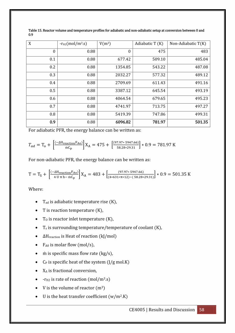
CE4005 | Results and Discussion 58
Table 15. Reactor volume and temperature profiles for adiabatic and non-adiabatic setup at conversion between 0 and 0.9
X -rH2(mol/m3.s) V(m3) Adiabatic T (K) Non-Adiabatic T(K)
0 0.88 0 475 483
0.1 0.88 677.42 509.10 485.04
0.2 0.88 1354.85 543.22 487.08
0.3 0.88 2032.27 577.32 489.12
0.4 0.88 2709.69 611.43 491.16
0.5 0.88 3387.12 645.54 493.19
0.6 0.88 4064.54 679.65 495.23
0.7 0.88 4741.97 713.75 497.27
0.8 0.88 5419.39 747.86 499.31
0.9 0.88 6096.82 781.97 501.35
For adiabatic PFR, the energy balance can be written as:
[(
] 47 [
( . .
. . ] 0.9 781.97
For non-adiabatic PFR, the energy balance can be written as:
[(
] 48 [
( . .
( ( . . ] 0.9 01. K
Where:
Tad is adiabatic temperature rise (K),
T is reaction temperature (K),
TO is reactor inlet temperature (K),
Ts is surrounding temperature/temperature of coolant (K),
ΔHreaction is Heat of reaction (kJ/mol)
FA0 is molar flow (mol/s),
is specific mass flow rate (kg/s),
CP is specific heat of the system (J/g mol.K)
XA is fractional conversion,
-rH2 is rate of reaction (mol/m3.s)
V is the volume of reactor (m3)
U is the heat transfer coefficient (w/m2.K)
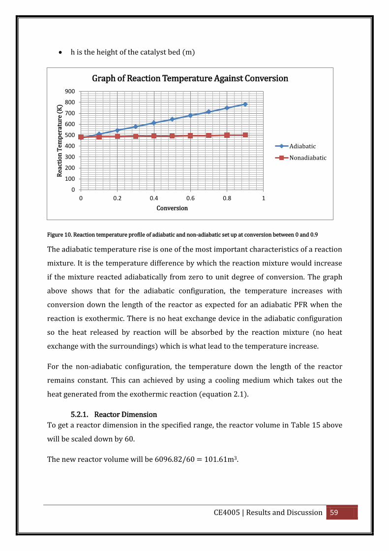
CE4005 | Results and Discussion 59
h is the height of the catalyst bed (m)
Figure 10. Reaction temperature profile of adiabatic and non-adiabatic set up at conversion between 0 and 0.9
The adiabatic temperature rise is one of the most important characteristics of a reaction
mixture. It is the temperature difference by which the reaction mixture would increase
if the mixture reacted adiabatically from zero to unit degree of conversion. The graph
above shows that for the adiabatic configuration, the temperature increases with
conversion down the length of the reactor as expected for an adiabatic PFR when the
reaction is exothermic. There is no heat exchange device in the adiabatic configuration
so the heat released by reaction will be absorbed by the reaction mixture (no heat
exchange with the surroundings) which is what lead to the temperature increase.
For the non-adiabatic configuration, the temperature down the length of the reactor
remains constant. This can achieved by using a cooling medium which takes out the
heat generated from the exothermic reaction (equation 2.1).
5.2.1. Reactor Dimension
To get a reactor dimension in the specified range, the reactor volume in Table 15 above
will be scaled down by 60.
The new reactor volume will be 6096.82/60 = 101.61m3.
0
100
200
300
400
500
600
700
800
900
0 0.2 0.4 0.6 0.8 1
Rea
ctio
n T
emp
erat
ure
(K
)
Conversion
Graph of Reaction Temperature Against Conversion
Adiabatic
Nonadiabatic
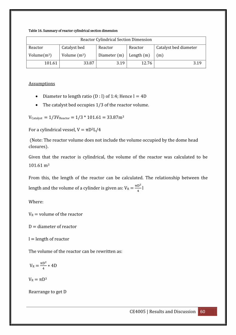
CE4005 | Results and Discussion 60
Table 16. Summary of reactor cylindrical section dimension
Reactor Cylindrical Section Dimension
Reactor
Volume(m3)
Catalyst bed
Volume (m3)
Reactor
Diameter (m)
Reactor
Length (m)
Catalyst bed diameter
(m)
101.61 33.87 3.19 12.76 3.19
Assumptions
Diameter to length ratio (D : l) of 1:4; Hence l 4D
The catalyst bed occupies 1/3 of the reactor volume.
VCatalyst = 1/3VReactor = 1/3 * 101.61 = 33.87m3
For a cylindrical vessel, V = πD2L/4
(Note: The reactor volume does not include the volume occupied by the dome head
closures).
Given that the reactor is cylindrical, the volume of the reactor was calculated to be
101.61 m3
From this, the length of the reactor can be calculated. The relationship between the
length and the volume of a cylinder is given as: VR =
l
Where:
VR = volume of the reactor
D = diameter of reactor
l = length of reactor
The volume of the reactor can be rewritten as:
VR =
4D
VR πD3
Rearrange to get D
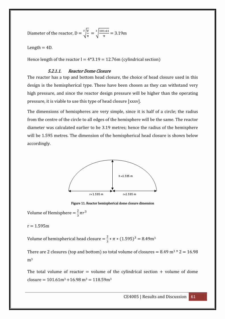
CE4005 | Results and Discussion 61
Diameter of the reactor, D = √
= √
.
= 3.19m
Length = 4D.
Hence length of the reactor l = 4*3.19 = 12.76m (cylindrical section)
5.2.1.1. Reactor Dome Closure
The reactor has a top and bottom head closure, the choice of head closure used in this
design is the hemispherical type. These have been chosen as they can withstand very
high pressure, and since the reactor design pressure will be higher than the operating
pressure, it is viable to use this type of head closure [xxxv].
The dimensions of hemispheres are very simple, since it is half of a circle; the radius
from the centre of the circle to all edges of the hemisphere will be the same. The reactor
diameter was calculated earlier to be 3.19 metres; hence the radius of the hemisphere
will be 1.595 metres. The dimension of the hemispherical head closure is shown below
accordingly.
Figure 11. Reactor hemispherical dome closure dimension
Volume of Hemisphere =
r = 1.595m
Volume of hemispherical head closure =
(1. 9 = 8.49m3
There are 2 closures (top and bottom) so total volume of closures = 8.49 m3 * 2 = 16.98
m3
The total volume of reactor = volume of the cylindrical section + volume of dome
closure = 101.61m3 +16.98 m3 = 118.59m3
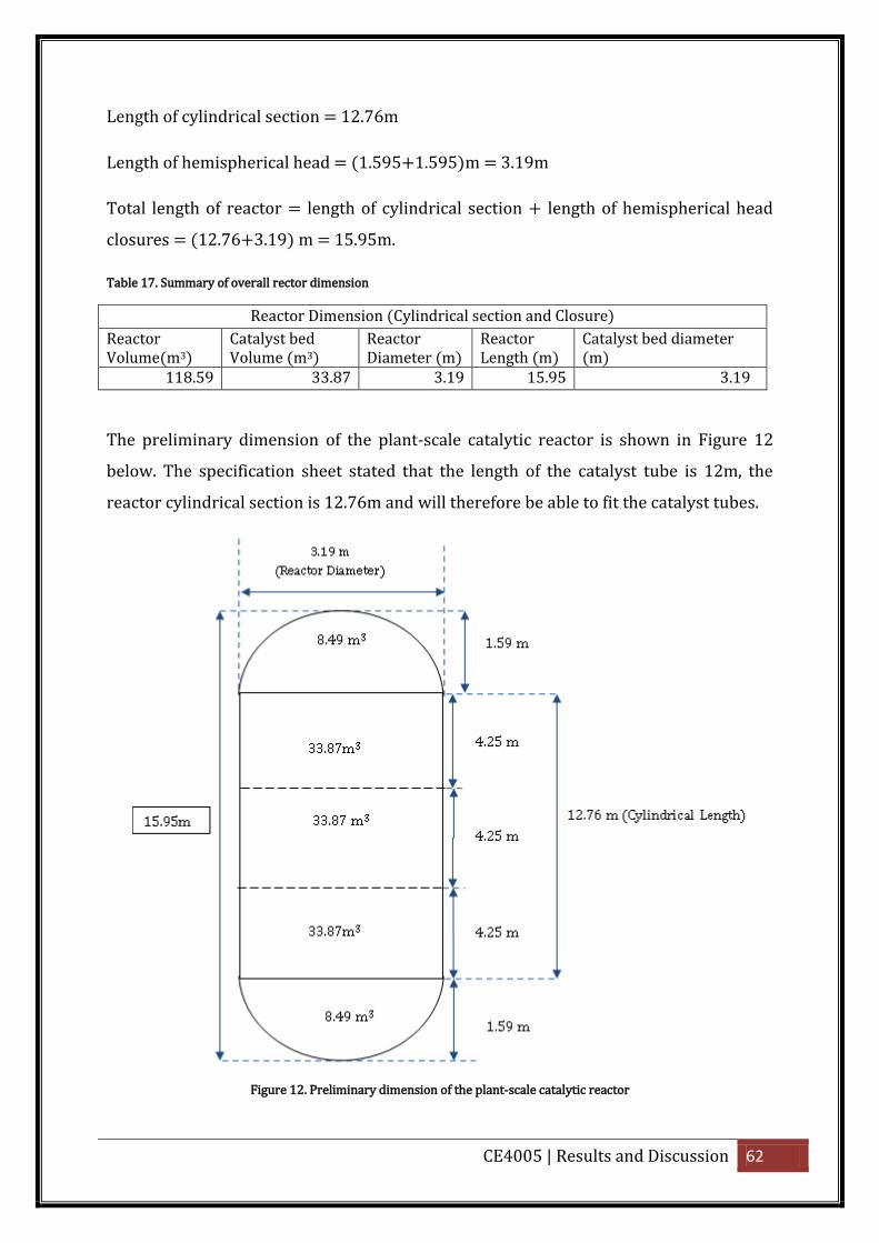
CE4005 | Results and Discussion 62
Length of cylindrical section = 12.76m
Length of hemispherical head = (1.595+1.595)m = 3.19m
Total length of reactor = length of cylindrical section + length of hemispherical head
closures = (12.76+3.19) m = 15.95m.
Table 17. Summary of overall rector dimension
Reactor Dimension (Cylindrical section and Closure)
Reactor Volume(m3)
Catalyst bed Volume (m3)
Reactor Diameter (m)
Reactor Length (m)
Catalyst bed diameter (m)
118.59 33.87 3.19 15.95 3.19
The preliminary dimension of the plant-scale catalytic reactor is shown in Figure 12
below. The specification sheet stated that the length of the catalyst tube is 12m, the
reactor cylindrical section is 12.76m and will therefore be able to fit the catalyst tubes.
Figure 12. Preliminary dimension of the plant-scale catalytic reactor
CE4005 | Results and Discussion 63
5.2.1.2. Catalyst Bed Characteristics
5.2.1.2.1. Catalyst Weight
Assuming a Cu/ZnO/Al2O3 catalyst is used, The bulk density, ρb of the catalyst is 1100
kg/m3 [xxxvi ]
WC = VC * ρb = 33.87 m3 * 1100 kg/m3 = 37257kg
Where: WC is weight of catalyst; VC is volume of catalyst and ρb is the catalyst bulk
density.
5.2.1.2.2. Number of tubes required for the catalyst
N olume of catalyst bed/(
i. d Length of catalyst tubes
N .87
π4 0.0 8
12 2489 tubes
5.2.1.2.3. Bed Depth
Weight of catalyst, Wc = 37257kg
Diameter of the reactor (D) = Catalyst bed diameter= 3.19m,
atalyst bulk density, ρ 1100kg/m3
Bed depth, L
. 4.2 m
5.2.1.2.4. Mass Velocity
Mass velocity, G
.
. 7.29 kgs m
5.2.1.2.5. Reynolds Number
For a spherical particle, the effective particle diameter, d’p= diameter of particle, dp =
0.00287m [ix]
e d G
0.00287 7.29
1.6 10 1 08
Re < 2000 hence the flow will be laminar and the profile of velocity will be parabolic.
5.2.1.2.6. Pressure Drop
Pressure drop ( P
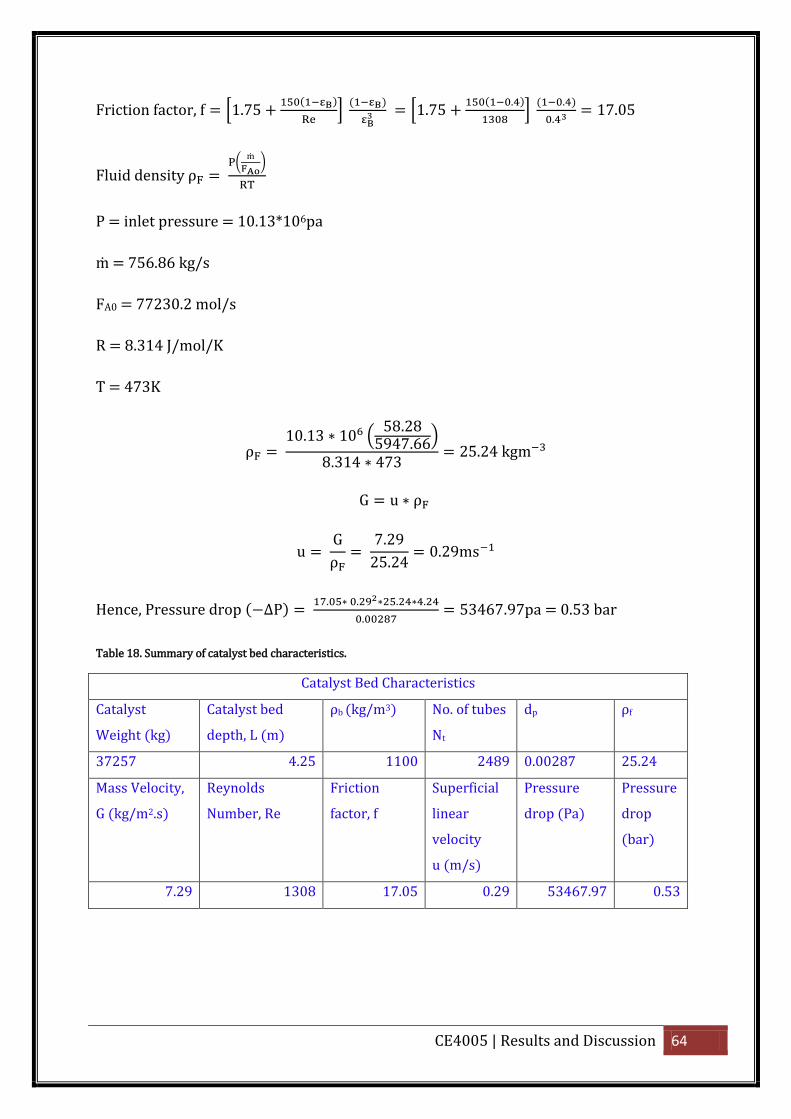
CE4005 | Results and Discussion 64
Friction factor, f [1.7 (
] (
[1.7
( .
] ( .
. 17.0
Fluid density ρ (
)
P = inlet pressure = 10.13*106pa
= 756.86 kg/s
FA0 = 77230.2 mol/s
R = 8.314 J/mol/K
T = 473K
ρ 10.1 10 (
8.28 947.66
)
8. 14 47 2 .24 kgm
G u ρ
u G
ρ 7.29
2 .24 0.29ms
Hence, Pressure drop ( P . . . .
. 467.97pa = 0.53 bar
Table 18. Summary of catalyst bed characteristics.
Catalyst Bed Characteristics
Catalyst
Weight (kg)
Catalyst bed
depth, L (m)
ρb (kg/m3) No. of tubes
Nt
dp ρf
37257 4.25 1100 2489 0.00287 25.24
Mass Velocity,
G (kg/m2.s)
Reynolds
Number, Re
Friction
factor, f
Superficial
linear
velocity
u (m/s)
Pressure
drop (Pa)
Pressure
drop
(bar)
7.29 1308 17.05 0.29 53467.97 0.53

CE4005 | Results and Discussion 65
5.2.1.2.6.1. Sensitivity to pressure drop
The sensitivity of the reactor dimension to a given pressure drop can be used for
operating power cost and vessel cost studies. Therefore a sensitivity analysis will be
carried out for the rector dimension obtained from the plant-scale catalytic reactor
simulation.
Pressure drop, ( P
Bed depth, L (
. .
. . . 4.2 m
D
D √
√
. .18m
Ranges of pressure drop have been selected around the calculated pressure drop. The
sensitivity result is tabulated in Table 19 below.
Table 19. Reactor dimension sensitivity to pressure drop
Pressure drop
(Pa)
Bed Depth
L (m)
D^2 Diameter
D (m)
10000 0.795122107 54.23839605 7.364672162
20000 1.590244214 27.11919802 5.207609627
30000 2.385366321 18.07946535 4.251995455
40000 3.180488428 13.55959901 3.682336081
53467.97 4.251356496 10.14409114 3.184978985
60000 4.770732642 9.039732675 3.00661482
70000 5.565854749 7.748342293 2.783584432
80000 6.360976856 6.779799506 2.603804813
Figure 13 below shows the sensitivity of the reactor dimension to pressure drop.
Diameter (D) decreases and the bed depth (L) increases. This suggests that for a given
amount of catalyst, a reduced pressure drop can be obtained by reducing the bed depth
at the expense of increasing the bed diameter. Although reducing the pressure drop will
reduce the operating power cost, it will increase the vessel cost.
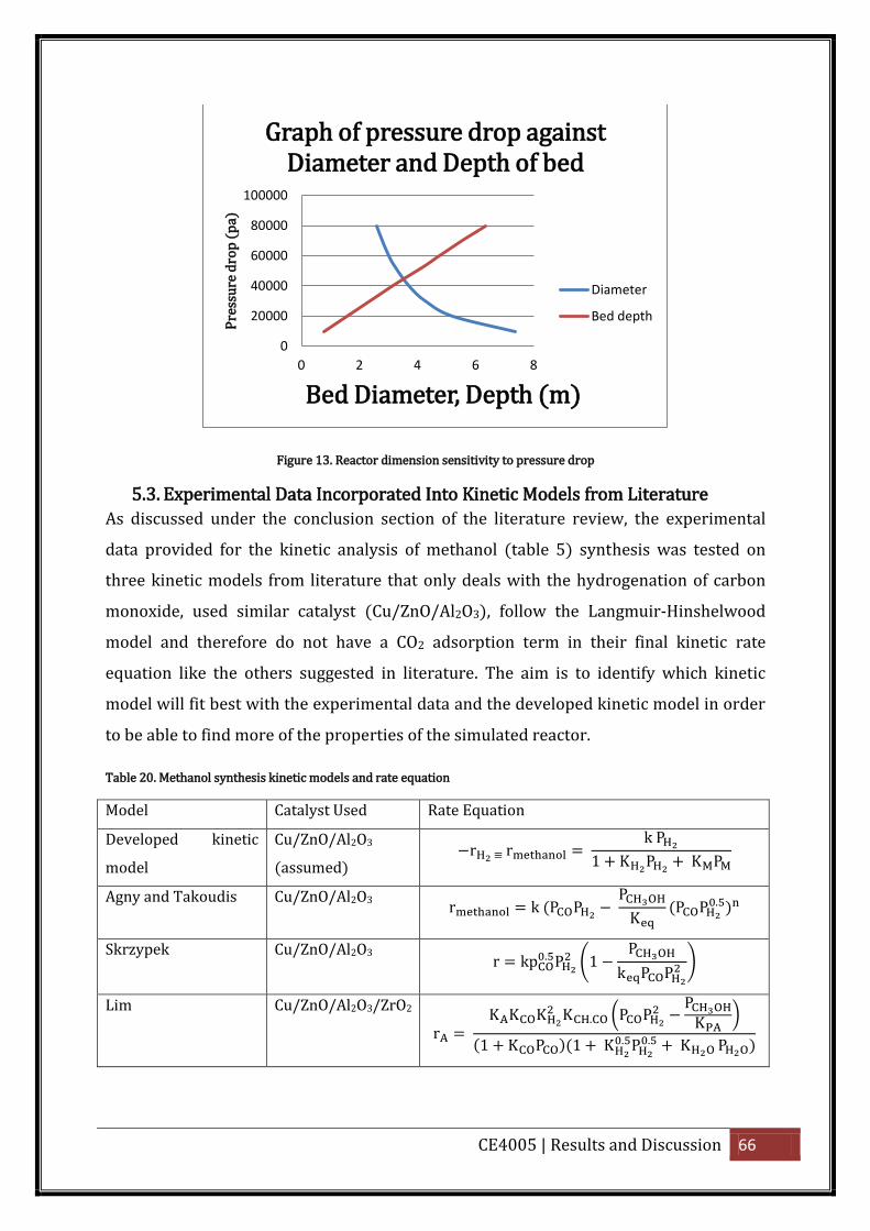
CE4005 | Results and Discussion 66
Figure 13. Reactor dimension sensitivity to pressure drop
5.3. Experimental Data Incorporated Into Kinetic Models from Literature
As discussed under the conclusion section of the literature review, the experimental
data provided for the kinetic analysis of methanol (table 5) synthesis was tested on
three kinetic models from literature that only deals with the hydrogenation of carbon
monoxide, used similar catalyst (Cu/ZnO/Al2O3), follow the Langmuir-Hinshelwood
model and therefore do not have a CO2 adsorption term in their final kinetic rate
equation like the others suggested in literature. The aim is to identify which kinetic
model will fit best with the experimental data and the developed kinetic model in order
to be able to find more of the properties of the simulated reactor.
Table 20. Methanol synthesis kinetic models and rate equation
Model Catalyst Used Rate Equation
Developed kinetic
model
Cu/ZnO/Al2O3
(assumed)
k P 1 P P
Agny and Takoudis Cu/ZnO/Al2O3 k (P P
P
(P P
.
Skrzypek Cu/ZnO/Al2O3 kp
. P (1
P
k P P )
Lim Cu/ZnO/Al2O3/ZrO2
. (P P
P
)
(1 P (1 . P
. P
0
20000
40000
60000
80000
100000
0 2 4 6 8
Pre
ssu
re d
rop
(p
a)
Bed Diameter, Depth (m)
Graph of pressure drop against Diameter and Depth of bed
Diameter
Bed depth
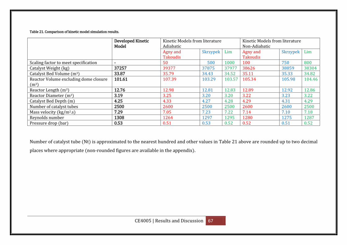
CE4005 | Results and Discussion 67
Table 21. Comparison of kinetic model simulation results.
Developed Kinetic Model
Kinetic Models from literature Adiabatic
Kinetic Models from literature Non-Adiabatic
Agny and Takoudis
Skrzypek Lim Agny and Takoudis
Skrzypek Lim
Scaling factor to meet specification - 50 500 1000 100 750 800 Catalyst Weight (kg) 37257 39377 37875 37977 38626 38859 38304 Catalyst Bed Volume (m3) 33.87 35.79 34.43 34.52 35.11 35.33 34.82 Reactor Volume excluding dome closure (m3)
101.61 107.39 103.29 103.57 105.34 105.98 104.46
Reactor Length (m3) 12.76 12.98 12.81 12.83 12.89 12.92 12.86 Reactor Diameter (m3) 3.19 3.25 3.20 3.20 3.22 3.23 3.22 Catalyst Bed Depth (m) 4.25 4.33 4.27 4.28 4.29 4.31 4.29 Number of catalyst tubes 2500 2600 2500 2500 2600 2600 2500 Mass velocity (kg/m2.s) 7.29 7.05 7.23 7.22 7.14 7.10 7.18 Reynolds number 1308 1264 1297 1295 1280 1275 1287 Pressure drop (bar) 0.53 0.51 0.53 0.52 0.52 0.51 0.52
Number of catalyst tube (Nt) is approximated to the nearest hundred and other values in Table 21 above are rounded up to two decimal
places where appropriate (non-rounded figures are available in the appendix).

CE4005 | Results and Discussion 68
Experiment 12 data (see Table 13 and Table 14) was used to simulate a plant scale
catalytic reaction at the specified reaction conditions, thermodynamic and physical
property.
The Agny and Takoudis kinetic model came out to be the best fit with the experimental
data as it required the least scaling factor (*50) in order to be similar to the results from
the simulation using the developed kinetic model. Agny and Takoudis model will
therefore be examined in detail and used later for Aspen modelling. The full results from
Skrzpek and Lim kinetic model can be found in appendix 6.
Using experiment 12 from the provided kinetic data, and following the steps in the
methodology (section 4.1.2), the kinetic simulation using the Agny and Takoudis kinetic
model is given in Table 22 below. The catalyst bed characteristics and sensitivity to
pressure drop will not be shown here as they are similar to those calculated in chapter
5.2 above (same trend and therefore same justification) but have been attached to
appendix 6. Values in Table 22 have been rounded up to two decimal place where
appropriate and therefore slightly differs from the corresponding table in the appendix.
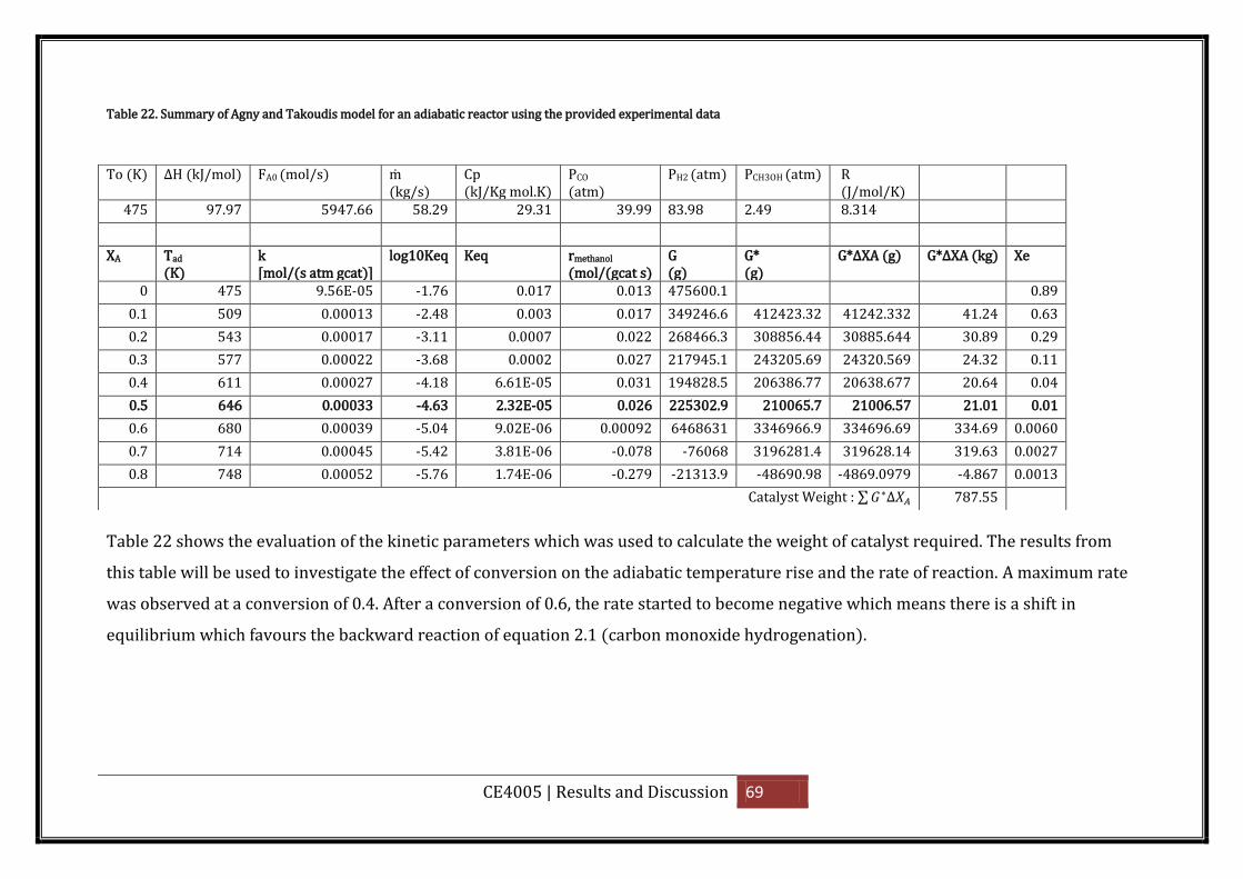
CE4005 | Results and Discussion 69
Table 22. Summary of Agny and Takoudis model for an adiabatic reactor using the provided experimental data
Table 22 shows the evaluation of the kinetic parameters which was used to calculate the weight of catalyst required. The results from
this table will be used to investigate the effect of conversion on the adiabatic temperature rise and the rate of reaction. A maximum rate
was observed at a conversion of 0.4. After a conversion of 0.6, the rate started to become negative which means there is a shift in
equilibrium which favours the backward reaction of equation 2.1 (carbon monoxide hydrogenation).
To (K) H (kJ/mol FA0 (mol/s) (kg/s)
Cp (kJ/Kg mol.K)
PCO
(atm) PH2 (atm) PCH3OH (atm) R
(J/mol/K)
475 97.97 5947.66 58.29 29.31 39.99 83.98 2.49 8.314
XA Tad (K)
k [mol/(s atm gcat)]
log10Keq Keq rmethanol
(mol/(gcat s) G (g)
G* (g)
G* (g G* (kg Xe
0 475 9.56E-05 -1.76 0.017 0.013 475600.1 0.89
0.1 509 0.00013 -2.48 0.003 0.017 349246.6 412423.32 41242.332 41.24 0.63
0.2 543 0.00017 -3.11 0.0007 0.022 268466.3 308856.44 30885.644 30.89 0.29
0.3 577 0.00022 -3.68 0.0002 0.027 217945.1 243205.69 24320.569 24.32 0.11
0.4 611 0.00027 -4.18 6.61E-05 0.031 194828.5 206386.77 20638.677 20.64 0.04
0.5 646 0.00033 -4.63 2.32E-05 0.026 225302.9 210065.7 21006.57 21.01 0.01
0.6 680 0.00039 -5.04 9.02E-06 0.00092 6468631 3346966.9 334696.69 334.69 0.0060
0.7 714 0.00045 -5.42 3.81E-06 -0.078 -76068 3196281.4 319628.14 319.63 0.0027
0.8 748 0.00052 -5.76 1.74E-06 -0.279 -21313.9 -48690.98 -4869.0979 -4.867 0.0013
Catalyst Weight : ∑ 787.55
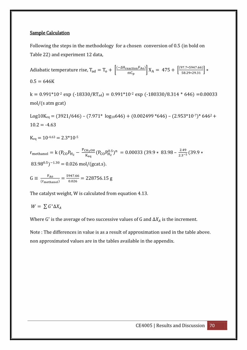
CE4005 | Results and Discussion 70
Sample Calculation
Following the steps in the methodology for a chosen conversion of 0.5 (in bold on
Table 22) and experiment 12 data,
Adiabatic temperature rise, [(
] 47 [
( . .
. . ]
0. 646
k = 0.991*10-2 exp (-18330/RTad) = 0.991*10-2 exp (-180330/8.314 * 646) =0.00033
mol/(s atm gcat)
Log10Keq = (3921/646) – (7.971* log10646) + (0.002499 *646) – (2.953*10-7)* 6462 +
10.2 = -4.63
Keq = 10-4.63 = 2.3*10-5
k (P P
(P P
. 0.000 ( 9.9 8 .98 – .
. ( 9.9
8 .98 . . = 0.026 mol/(gcat.s).
G
( .
. 2287 6.1 g
The catalyst weight, W is calculated from equation 4.13.
∑
Where G* is the average of two successive values of G and is the increment.
Note : The differences in value is as a result of approximation used in the table above.
non approximated values are in the tables available in the appendix.
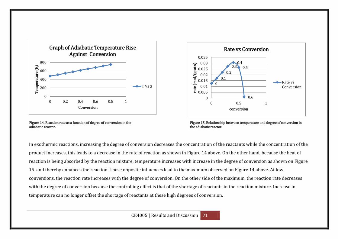
CE4005 | Results and Discussion 71
0
0.1
0.2
0.3 0.4
0.5
0.6 0
0.005
0.01
0.015
0.02
0.025
0.03
0.035
0 0.5 1
rate
(m
ol/
(gca
t s)
conversion
Rate vs Conversion
Rate vsConversion
0
200
400
600
800
0 0.2 0.4 0.6 0.8 1
Tem
per
atu
re (
K)
Conversion
Graph of Adiabatic Temperature Rise Against Conversion
T Vs X
In exothermic reactions, increasing the degree of conversion decreases the concentration of the reactants while the concentration of the
product increases, this leads to a decrease in the rate of reaction as shown in Figure 14 above. On the other hand, because the heat of
reaction is being absorbed by the reaction mixture, temperature increases with increase in the degree of conversion as shown on Figure
15 and thereby enhances the reaction. These opposite influences lead to the maximum observed on Figure 14 above. At low
conversions, the reaction rate increases with the degree of conversion. On the other side of the maximum, the reaction rate decreases
with the degree of conversion because the controlling effect is that of the shortage of reactants in the reaction mixture. Increase in
temperature can no longer offset the shortage of reactants at these high degrees of conversion.
Figure 15. Relationship between temperature and degree of conversion in the adiabatic reactor.
Figure 14. Reaction rate as a function of degree of conversion in the adiabatic reactor.
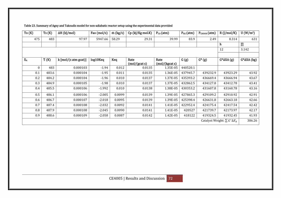
CE4005 | Results and Discussion 72
Table 23. Summary of Agny and Takoudis model for non-adiabatic reactor setup using the experimental data provided
To (K) Ts (K) H (kJ/mol Fao (mol/s) (kg/s Cp (kJ/Kg mol.K) PCO (atm) PH2 (atm) PCH3OH (atm) R (J/mol/K) U (W/m2)
475 483 97.97 5947.66 58.29 29.31 39.99 83.9 2.49 8.314 631
h ∏
12 3.142
XA T (K) k [mol/(s atm gcat)] log10Keq Keq Rate (mol/(gcat s)
Rate (mol/(kgcat s)
G (g) G* (g) G* (g G* (kg
0 483 0.000103 -1.94 0.012 0.0135 1.35E-05 440520.1
0.1 483.6 0.000104 -1.95 0.011 0.0135 1.36E-05 437945.7 439232.9 43923.29 43.92
0.2 484.2 0.000104 -1.96 0.010 0.0137 1.37E-05 435393.2 436669.4 43666.94 43.67
0.3 484.9 0.000105 -1.98 0.010 0.0137 1.37E-05 432862.5 434127.8 43412.78 43.41
0.4 485.5 0.000106 -1.992 0.010 0.0138 1.38E-05 430353.2 431607.8 43160.78 43.16
0.5 486.1 0.000106 -2.005 0.0099 0.0139 1.39E-05 427865.3 429109.2 42910.92 42.91
0.6 486.7 0.000107 -2.018 0.0095 0.0139 1.39E-05 425398.4 426631.8 42663.18 42.66
0.7 487.4 0.000108 -2.032 0.0092 0.0141 1.41E-05 422952.4 424175.4 42417.54 42.42
0.8 487.9 0.000108 -2.045 0.0090 0.0141 1.41E-05 420527 421739.7 42173.97 42.17
0.9 488.6 0.000109 -2.058 0.0087 0.0142 1.42E-05 418122 419324.5 41932.45 41.93
Catalyst Weight: ∑ 386.26
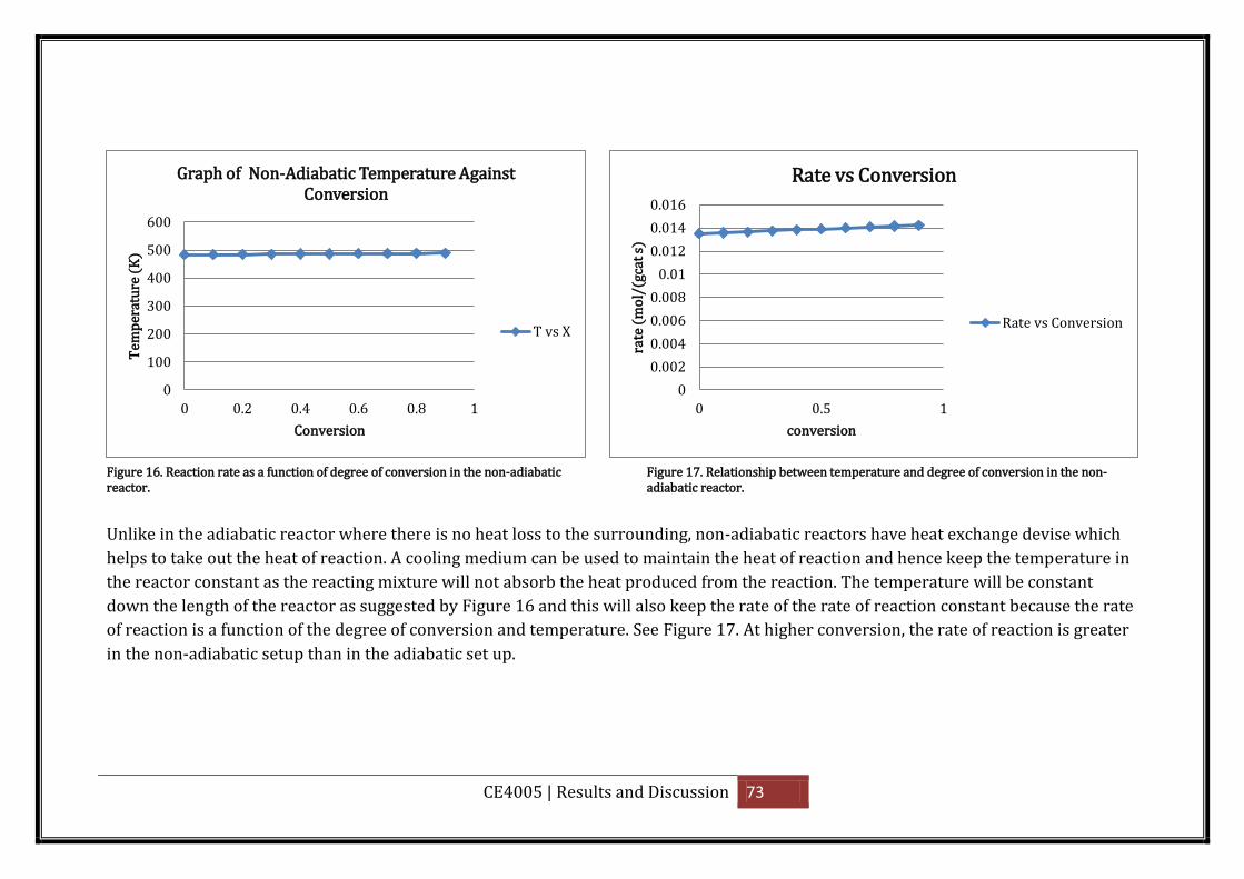
CE4005 | Results and Discussion 73
0
100
200
300
400
500
600
0 0.2 0.4 0.6 0.8 1
Tem
per
atu
re (
K)
Conversion
Graph of Non-Adiabatic Temperature Against Conversion
T vs X
0
0.002
0.004
0.006
0.008
0.01
0.012
0.014
0.016
0 0.5 1
rate
(m
ol/
(gca
t s)
conversion
Rate vs Conversion
Rate vs Conversion
Unlike in the adiabatic reactor where there is no heat loss to the surrounding, non-adiabatic reactors have heat exchange devise which
helps to take out the heat of reaction. A cooling medium can be used to maintain the heat of reaction and hence keep the temperature in
the reactor constant as the reacting mixture will not absorb the heat produced from the reaction. The temperature will be constant
down the length of the reactor as suggested by Figure 16 and this will also keep the rate of the rate of reaction constant because the rate
of reaction is a function of the degree of conversion and temperature. See Figure 17. At higher conversion, the rate of reaction is greater
in the non-adiabatic setup than in the adiabatic set up.
Figure 16. Reaction rate as a function of degree of conversion in the non-adiabatic reactor.
Figure 17. Relationship between temperature and degree of conversion in the non-adiabatic reactor.
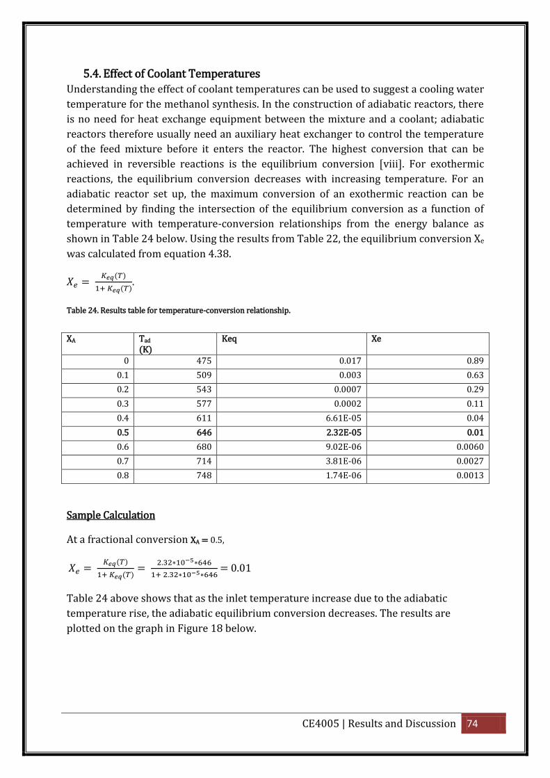
CE4005 | Results and Discussion 74
5.4. Effect of Coolant Temperatures
Understanding the effect of coolant temperatures can be used to suggest a cooling water
temperature for the methanol synthesis. In the construction of adiabatic reactors, there
is no need for heat exchange equipment between the mixture and a coolant; adiabatic
reactors therefore usually need an auxiliary heat exchanger to control the temperature
of the feed mixture before it enters the reactor. The highest conversion that can be
achieved in reversible reactions is the equilibrium conversion [viii]. For exothermic
reactions, the equilibrium conversion decreases with increasing temperature. For an
adiabatic reactor set up, the maximum conversion of an exothermic reaction can be
determined by finding the intersection of the equilibrium conversion as a function of
temperature with temperature-conversion relationships from the energy balance as
shown in Table 24 below. Using the results from Table 22, the equilibrium conversion Xe
was calculated from equation 4.38.
(
( .
Table 24. Results table for temperature-conversion relationship.
Sample Calculation
At a fractional conversion XA = 0.5,
(
(
.
. = 0.01
Table 24 above shows that as the inlet temperature increase due to the adiabatic
temperature rise, the adiabatic equilibrium conversion decreases. The results are
plotted on the graph in Figure 18 below.
XA Tad (K)
Keq Xe
0 475 0.017 0.89
0.1 509 0.003 0.63
0.2 543 0.0007 0.29
0.3 577 0.0002 0.11
0.4 611 6.61E-05 0.04
0.5 646 2.32E-05 0.01
0.6 680 9.02E-06 0.0060
0.7 714 3.81E-06 0.0027
0.8 748 1.74E-06 0.0013
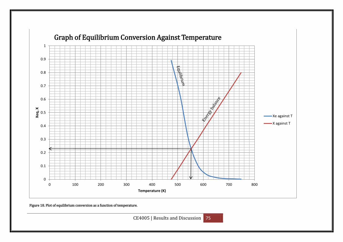
CE4005 | Results and Discussion 75
Figure 18. Plot of equilibrium conversion as a function of temperature.
0
0.1
0.2
0.3
0.4
0.5
0.6
0.7
0.8
0.9
1
0 100 200 300 400 500 600 700 800
Xe
q, X
Temperature (K)
Graph of Equilibrium Conversion Against Temperature
Xe against T
X against T
CE4005 | Results and Discussion 76
Figure 18 shows that for a feed temperature of 475K, the adiabatic temperature
equilibrium is about 550K and the equilibrium conversion is 23% therefore a cooling
water temperature of 550K will be required on the shell side of the reactor to keep the
reaction at the equilibrium conversion (highest conversion that can be achieved) .
Cooling the feed down to 400K will shift the energy balance line to the left and increase
the equilibrium conversion. Interstage cooling can be used to achieve higher
conversions.
Figure 19. Interstage cooling [xxxvii].
Interstage cooling can be used to get the best result from the reaction rate and reactant
conversion. Conversion is much less at lower temperature, this means catalyst mass and
volume must be much greater. It is very expensive to operate reactors at high
temperature and pressure, so smaller volume of reactor will be cost effective. The
cooler allows the temperature during a reaction to drop whilst not affecting the
pressure or the stream composition. This significant property is a good way of
increasing conversion and maximising productivity without an increase in overall
reactor volume [xxxvii].
5.5. Modelling with ASPEN Process Modelling Software
Using the thermodynamic and physical property data provided in the brief as well as
results from the reactor simulation from the developed kinetic rate equation, an
adiabatic reactor was modelled on ASPEN. The PSRK property method was selected as
it is suitable for reversible exothermic reactions at high temperature and pressure such
as the methanol synthesis reaction. The reactor model summary is provided below.
CE4005 | Results and Discussion 77
Figure 20. Reactor model summary
The flow sheet and the stream results from the simulation for a feed composition of
70% H2 and 30% CO entering the reactor at 473K (200 C) is given below.
CE4005 | Results and Discussion 78
Figure 21. Flow sheet with heat and material balance for ASPEN simulation at a feed inlet temperature of 473K (200 C)
An adiabatic reactor can be controlled by either the composition of the feed or the feed
temperature. Varying the composition showed that a feed composition of 70% H2 and
30% CO is optimum for methanol synthesis under the specified conditions. A conversion
of 29% was achieved (mole flow of methanol produced/ mole flow of feed *100 =
[{6238.968/21412.800} *100]) the results of varying the feed composition and the
temperature and composition profile resulting from such variation has been attached to
the appendix. In order for the reaction to occur, the molar composition of H2 must
always be greater than that of CO following from the stoichiometry of equation 2.1
(carbon monoxide hydrogenation).
PFRB2 B3
1 2 3 4
Heat and Material Balance Table
Stream ID 1 2 3 4
Temperature C 199.8 199.8 1182.7 1182.7
Pressure bar 101.300 101.300 101.300 100.800
Vapor Frac 1.000 1.000 1.000 1.000
Mole Flow kmol/hr 21412.800 21412.800 8934.864 8934.864
Mass Flow kg/hr 210150.271 210150.271 210150.271 210150.271
Volume Flow cum/hr 8977.323 8977.323 11067.410 11120.577
Enthalpy Gcal/hr -142.218 -142.218 -142.218 -142.218
Mole Flow kmol/hr
CO 6423.840 6423.840 184.872 184.872
H2 14988.960 14988.960 2511.024 2511.024
CH4O 6238.968 6238.968
CE4005 | Results and Discussion 79
Figure 22. Temperature profile of the reactor at a feed composition of 70% H2 and 30% CO
The temperature profile above shows that most of the reaction occurs at the entrance of the reactor. This points towards the need for a
cooling medium to cool the reactant down so that conversion to methanol can occur slowly along the length of the reactor. The adiabatic
temperature rise in this simulation is very high and therefore, there is a need to understand the effect that various feed temperature will
have on this simulation. This vital information can be obtained from a sensitivity analysis with varying feed temperature.
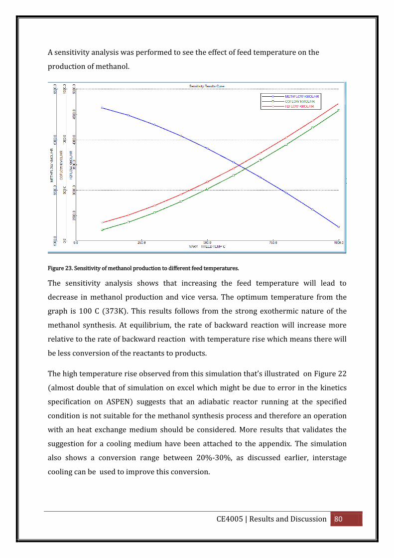
CE4005 | Results and Discussion 80
A sensitivity analysis was performed to see the effect of feed temperature on the
production of methanol.
Figure 23. Sensitivity of methanol production to different feed temperatures.
The sensitivity analysis shows that increasing the feed temperature will lead to
decrease in methanol production and vice versa. The optimum temperature from the
graph is 100 C (373K). This results follows from the strong exothermic nature of the
methanol synthesis. At equilibrium, the rate of backward reaction will increase more
relative to the rate of backward reaction with temperature rise which means there will
be less conversion of the reactants to products.
he high tempe atu e ise obse ved f om this simulation that’s illust ated on Figure 22
(almost double that of simulation on excel which might be due to error in the kinetics
specification on ASPEN) suggests that an adiabatic reactor running at the specified
condition is not suitable for the methanol synthesis process and therefore an operation
with an heat exchange medium should be considered. More results that validates the
suggestion for a cooling medium have been attached to the appendix. The simulation
also shows a conversion range between 20%-30%, as discussed earlier, interstage
cooling can be used to improve this conversion.
CE4005 | Results and Discussion 81
5.6. Further Discussion
To describe the behaviour of a chemical reactor, the composition and temperature at
each point of the reactor throughout the course of the chemical reaction must be known.
Concentration of species however can change at any point either due to disappearance
by chemical reaction or via mass transfer. Analogously, the temperature at any point
may change because heat is being absorbed or released by chemical reaction or by heat
transfer. Hence the concentration and temperature of a given spot in a reactor is
affected by the rate of the chemical reaction as well as the heat and mass transfer.
Reaction rate is determined by the micro kinetic properties which influence the
outcome of a process through the kinetics of heat and mass transfer.
A continuous adiabatic plug flow reactor (PFR) does not have the effect of macro kinetic
properties, hence the size and shape of the reactor is immaterial from the viewpoint of
chemical reaction. This makes direct data transfer possible i.e. the possibility to carry
out an experiment in a small laboratory scale reactor and transfer the result to a full
plant-scale industrial reactor of the same type preserving identical external reaction
conditions and inlet composition of the reaction mixture [xxxviii].
With regards to the developed kinetics, it was assumed that the reaction is irreversible
which isn’t the case as the methanol synthesis eaction is indeed eve sible. At the
operating conditions used for the methanol synthesis, the ideality assumed will be
invalid due to the non-ideal behaviour of gases at these conditions, the non ideality will
require fugacity parameters to be included in the kinetic rate equation to be in the
formed developed by Natta et.al (1953). Other side reactions discussed in the literature
review such as the water gas shift reaction and formation of DME are also very likely to
occur and these will have an impact on the rate of reaction. These factors put a lot of
limit to the developed kinetic rate equation and hence the performance of the reactor
simulated from that kinetic model.
CE4005 | Conclusion 82
6. Conclusion The primary objectives of this research project is to develop a kinetic model and reactor
design for the synthesis of methanol. Using the kinetic analysis data provided for
methanol synthesis, a Langmuir-Hinshelwood type of kinetics was developed. The
developed kinetic rate equation was used to simulate a plant scale catalytic reactor at
specified reaction conditions similar to that used in the chemical industry for methanol
synthesis. The reactor was simulated as a simple, one-dimensional, plug-flow, pseudo
homogeneous, nonisothermal reactor model.
Plug flow is an idealised flow of fluids under which all particles on a given cross section
will have identical velocity and direction of motion. This excludes mixing in the
direction of motion. Ideal gas law was assumed for all calculations in this report. Under
plug flow, particles of different age do not mix, as the particles that enter the reactor at
the same time must leave simultaneously. In real reactors, the flow of fluids can only
approximate to plug flow. The Reynolds number was calculated to be less than 2000 (Re
< 2000) which means the flow is laminar and this will result in a velocity p ofile that’s
parabolic. In a parabolic velocity profile, the molecules on a given cross section do not
move at the same velocity so particles of different age will therefore mix to some extent.
The effect of mixing can be regarded as negligible if the mixing does not significantly
alter the concentration field induced by chemical reaction given that there are no
appreciable longitudinal gradients of conversion within the reactor. However, because
the length of the tube along which the major portion of the reactant has been converted
to methanol is much larger than the tube diameter (ratio of 1:315), the concept of plug
flow is realistic. The maximum adiabatic temperature on the excel simulation was 748K,
when the simulation was repeated on ASPEN, this value doubled for the same feed
composition and specification. It is not advisable to use adiabatic reactors for reactions
whose adiabatic temperature rise is very large. Isothermal operation will be preferable
as this will allow the reaction to take place at a lower temperature which is more
favourable from the point of view of chemical equilibrium. The reactor was also
modelled to operate non-adiabatically and higher rate was observed at higher
conversion values than in the adiabatic setup. The non-adiabatic temperature profile
which allows for heat transfer agrees more with the admissible temperature range from
literature and the temperature at which the experimental data used was carried out.
The equilibrium conversion for the earlier simulation for the adiabatic setup was 23%
CE4005 | Conclusion 83
for a feed temperature of 473K. ASPEN confirms this result as the range of methanol
conversion lies between 20% and 30 %. Interstage cooling was suggested in order to
achieve higher conversion of the reactants to methanol. Adiabatic plug flow reactor can
only be used if the temperature rise corresponding to the outlet degree of conversion
remains smaller than the operating temperature region of the reactor. The operating
temperature of the methanol synthesis is between 400-700K from literature, see Table
2. The adiabatic temperature rise from the reactor simulation exceeds this value at the
specified conditions. It is important to optimise the temperature regime due to the
effect of temperature on the rate of reaction. Optimisation of the temperature regime
will be discussed further under the recommendation section.
The objectives of this research project were met and I had the opportunity to develop
kinetic modelling methods and approaches, on this basis this research can be concluded
as being successful.
CE4005 | Recommendations 84
7. Recommendations At equilibrium, the rate of forward reaction is equal to the rate of backward reaction.
For exothermic reactions, the rate of backward reaction will increase more relative to
the rate of backward reaction with temperature rise, therefore lowering the equilibrium
conversion and subsequently the rate of reaction. For a gas reversible exothermic
reaction such as the methanol synthesis, the productivity of the reactor for a given inlet
composition is at its maximum if the state of the reaction mixture follows the path of
maximum productivity. This path is approached neither by the adiabatic nor the
isothermal temperature regime. For the adiabatic setup, increase in temperature of the
reaction mixture favours the rate of the reaction but the productivity is low because the
reaction mixture rapidly approaches the region of the effect of thermodynamic
equilibrium at high temperature. In an isothermal reactor, the reaction can take place at
lower temperature which is more favourable from the point of view of chemical
equilibrium. However the reactor productivity will remain low because of the low
reaction rate in the region free of the effect of chemical equilibrium.
In a eacto that’s neither adiabatic nor isothermal, the temperature profile can be
adjusted such that the reaction mixture is allowed to be heated by the heat of reaction in
the region free of the effect of chemical equilibrium, to be later cooled by heat exchange
in the region affected strongly by chemical equilibrium. This leads to interstage cooling.
Low conversion is sometimes overcome by using several adiabatic reactors with
interstage cooling. Several reactors, with heat exchangers for cooling between them, are
run up to near the maximum reaction rate until satisfactory conversion is attained. This
is a common technique used in methanol synthesis from syngas. Interstage cooling
helps to achieve high conversion and extract reaction heat. Usually, up to three adiabatic
reactors with interstage cooling are sufficient to achieve good conversion [xxxix].
The optimum temperature regime for the methanol synthesis and other reversible
exothermic reaction will be that which approaches as closely as possible to the path of
maximum productivity without exceeding either the upper or the lower limit of the
admissible temperature range.
One of the advantages of the plug flow reactor which makes it suitable for gas phase
reactions is that it has no moving parts and therefore easy to maintain. Also, plug flow
reactors produce the highest conversion per reactor volume of any of the flow reactors.
CE4005 | Recommendations 85
However, for exothermic reactions, the temperature control is difficult and hotspots
might occur. Although the cost of the reactor and catalyst regeneration is high, using a
fluidised bed reactor can eliminate problems with hotspots as the contents in a fluidised
bed reactor are well mixed, resulting in a uniform temperature. A fluidised bed reactor
can handle large amounts of feed and solids and therefore will be suitable for the
methanol synthesis.
Finally, the method of obtaining the kinetic parameters can be improved by solving
them numerically with software package such as POLYMATH or MATLAB. This will give
an improved kinetic model and hence reduce errors in the reactor design and
performance.
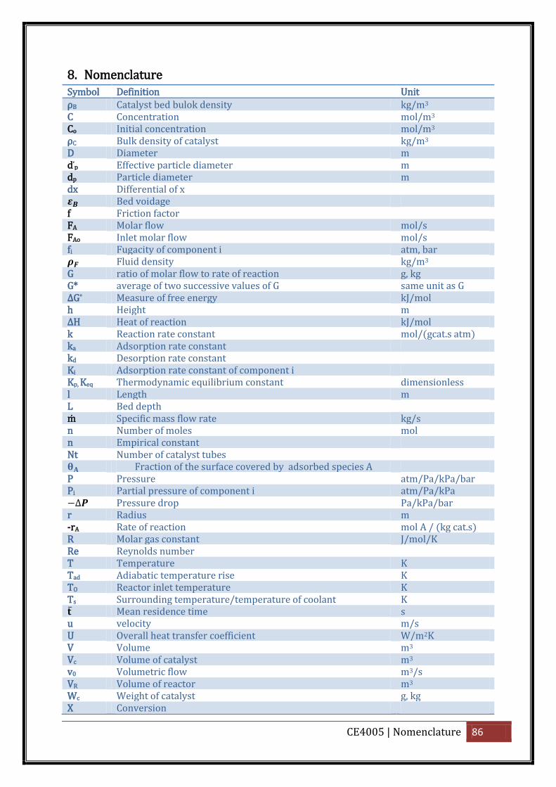
CE4005 | Nomenclature 86
8. Nomenclature Symbol Definition Unit ρB Catalyst bed bulok density kg/m3 C Concentration mol/m3 Co Initial concentration mol/m3 ρC Bulk density of catalyst kg/m3 D Diameter m d’p Effective particle diameter m dp Particle diameter m dx Differential of x Bed voidage f Friction factor FA Molar flow mol/s FAo Inlet molar flow mol/s fi Fugacity of component i atm, bar Fluid density kg/m3 G ratio of molar flow to rate of reaction g, kg G* average of two successive values of G same unit as G ΔG° Measure of free energy kJ/mol h Height m ΔH Heat of reaction kJ/mol k Reaction rate constant mol/(gcat.s atm) ka Adsorption rate constant kd Desorption rate constant Ki Adsorption rate constant of component i Kp, Keq Thermodynamic equilibrium constant dimensionless l Length m L Bed depth Specific mass flow rate kg/s n Number of moles mol n Empirical constant Nt Number of catalyst tubes action of the su face cove ed by adso bed species P Pressure atm/Pa/kPa/bar Pi Partial pressure of component i atm/Pa/kPa Pressure drop Pa/kPa/bar r Radius m -rA Rate of reaction mol A / (kg cat.s) R Molar gas constant J/mol/K Re Reynolds number T Temperature K Tad Adiabatic temperature rise K TO Reactor inlet temperature K Ts Surrounding temperature/temperature of coolant K Mean residence time s u velocity m/s U Overall heat transfer coefficient W/m2K V Volume m3 Vc Volume of catalyst m3 v0 Volumetric flow m3/s VR Volume of reactor m3 Wc Weight of catalyst g, kg X Conversion

CE4005 | References 87
Xe Equilibrium conversion
9. References i George A. Olah (2005). "Beyond Oil and Gas: The Methanol Economy". Angewandte
Chemie International Edition 44 (18): 2636–2639.
ii John J. McKetta Jr. Encyclopedia of Chemical Processing and Design. Volume 1:
Abrasives to Acrylonitrile. 1 Edition. CRC Press, 1976, pp. 418-451.
iii How is Methanol Made? - Methanol Institute . 2012. How is Methanol Made? -
Methanol Institute . [ONLINE] Available at: http://www.methanol.org/Methanol-
Basics/Overview/How-is-Methanol-Made-.aspx. [Accessed 29 October 2012].
iv Martyn V. Twigg. Catalyst Handbook. 2nd Edition., CRC Press, 1989, pp.442.
v F. Marschner and F. W. Moeller in Applied Industrial Catalysis, Vol. 2, Academic, New
York, 1983, pp. 215-243.
vi Strelzoff, S., "Methanol: Its Technology and Economics", Chem. Eng.Prog. Symp. Series,
No. 98, 66, 54-68 (1970).
vii Routes for making methanol from the full range of feedstocks 2012. . [ONLINE]
Available at: http://two.web-
dms.net/dms/uploaded_files/zerom/ZeroMDMS.mdb/documents/Routes%20for%20
making%20methanol%20new.pdf. [Accessed 29 October 2012].
viii Fogler, H. Scott. Elements of Chemical Reaction Engineering. 4th Ed., Englewood
Cliffs, N.J.: Prentice-Hall, 2008, pp. 15-20.
ix Dr. James Titiloye, (2011) Reaction Engineering 2 lecture notes, Aston University:
Department of Chemical Engineering and Applied Science.
x Octave Levenspiel, 1998. Chemical Reaction Engineering, 3rd Edition. Wiley.
xi A Novel Process for Heavy Residue Hydroconversion Using a Recoverable
Pseudohomogeneous Catalyst (PHC) System. [ONLINE] Available
at:http://www.onepetro.org/mslib/servlet/onepetropreview?id=SPE-117710-
MS&soc=SPE. [Accessed 29 October 2012].
xii Lurgi (1995). Integrated low pressure methanol process. Technical report. Lurgi Öl
Gas Chemie BmbH. Frankfurt am Main, Germany.
xiii Ingvild Lovik (200 ., “Modelling, Estimation and Optimization of he Methanol
Synthesis with Catalyst Deactivation.
CE4005 | References 88
xiv R. G Herman, K. Klier, G. W. Simmons, B. P. Finn, J.B Bulko, and T. P. Kobylinski,
"Catalytic Synthesis of Methanol from CO/H2. I. Phase Composition, Electronic
Properties, and Activity of the Cu/ZnO/M2O3 Catalysts," J. Catal., 56, 407-429 (1979).
xv S. Mehta, G. . Simmons, . lie , and . G. He man, “ he atalytic Synthesis of
Methanol f om O/H2”. J. Catal., 57, 339-360 (1979).
xvi . Deluza che, . ieffe , and . Muth, “Reactions CO, H2 - Synthese du Methanol sur
Chromite de Zinc Etude d'especes Chimisorbees a la Surface du Catalyseur Schemas
Reactionnels Possibles. ” Tetrahedron Letters., (38), 3585 (1977).
xvii H. H. ung, “Methanol Synthesis” atal. ev. – Sci. Eng., 22(2), 235-259 (1980).
xviii . gny and . G. akoudis, “Synthesis of Methanol f om a bon Mono ide and
Hydrogen over a Copper-Zinc Oxide- lumina atalyst”. Ind. Eng. hem., p od. es. Dev.,
24, 50-55 (1985).
xix G. Henrici-Olive and S. Olive, “Mechanistic eflections on the Methanol Synthesis
ith u/Zn atalysts”. J. Mol. atal., 17, 89-92 (1982).
xx . M. awa ah and . S. Hansen, “ inetics and Mechanism of Methanol
Decomposition Over Zinc-O ide” J. atal., 94, 175-186 (1985).
xxi J. . Edwa ds and G. L. Sch ade , “Inf a ed Spect oscopy of oppe /Zinc O ide
Catalysts for the Water-Gas Shift eaction and Methanol Synthesis”. J. atal., 94, 17 -
186 (1985).
xxii Y. B. Kagan, A.Y. Rozovskii, G. I. Lin, E. V. Sliviniskii, S. M. Loktev, L. G. Liberov, and A.
N. Bashki ov, “Mechanism fo the Synthesis of Methanol” inetics and atal., 16( , 809
(1975).
xxiii Y. B. Kagan, A.Y. Rozovskii, G. I. Lin, E. V. Sliviniskii, S. M. Loktev, L. G. Liberov, and
A. N. Bashkirov, “ he Mechanism of the Synthesis of Methanol f om a bon Dio ide and
Hyd ogen 1. inetic egula ities”, inetics and catal., 17( , 1 14-1320 (1976).
xxiv G. C. Chinchen, P. J, Denny, D. G. Parker, G. D. Short, M. S. Spencer, K. C. Waugh and
D. . han, “ he Activity of Cu-ZnO- l2O Methanol Synthesis atalysts”, P ep . Div.
Fuel Chem., ACS, 29(5), 178-188 (1984)
xxv M. Bowke , H. Houghton, and . . augh, “Mechanism and inetics of Methanol
Synthesis on Zinc O ide” J. hem. Soc., a aday ans. I. 77, 02 (1981).
xxvi H. Lim, M. J Pa k, S. H. ang, H. J. hae, J. . Bae and . . Jun, “Modeling of the
Kinetics for Methanol Synthesis using Cu/ZnO/Al2O3/ZrO2Catalyst: Influence of
Carbon Dioxide during Hydrogenation” Ind . Eng. hem. es. 2009, 48 (2 , pp. 10448-
10455
CE4005 | References 89
xxvii . N. . Bos, P. . Bo man, M. uczynski and . . este te p, “ he inetics of he
Methanol Synthesis on a oppe atalyst: n E pe imental Study”. hemical
Engineering Science. Vol. 44, No. 11, pp. 2435-2449, 1989.
xxviii G. Natta, p. Pino, G. Mazzanti, and I. Pasquon, “ inetic inte p etations of
heterogeneous catalysis and their application to reaction between gases at high
p essu e” 1. Synthesis of methanol. him. Ind., , 70 (19 .
xxix . lie , . hatikavanig, . G. He man, and G. . Simmons, “ atalytic Synthesis of
methanol f om O/H2 : 1 . Effects of ca bon dio ide,” J. atal., 74, 4 -360 (1982).
xxx A. Y. Rozovskii, khim. Prom., 11, 652-654 (1980).
xxv Rahman, Daaniya, "Kinetic Modeling Of Methanol Synthesis From Carbon Monoxide,
Carbon Dioxide, And Hydrogen Over A Cu/ ZnO/Cr2O3 Catalyst" (2012). Master's
Theses. Paper 4162.
xxxi J. Sk zypek, M. G zesik, and . Szopa, “Analysis of the low-temperature methanol
synthesis in a single commercial isothermal Cu-Zn-Al catalyst pellet using the dusty-gas
diffusion model” hemical Enginee ing Science, Volume 40, Issue 4, Pages 671-673,
(1985).
xxxii H. Lim, M.J Pa k, H. J. hae, J. . Bae and . . Jun, “Modelling of the kinetics for
methanol synthesis using Cu/ZnO/Al2O3/ZrO2 catalyst : influence of carbon dioxide
du ing hyd ogenation” Ind. Eng. hem. es. 2009, 48 (2 , pp. 10448-10455.
xxxiii R. K.Sinnott (2005) Mechanical design of process equipment: Choice of closure. R.
K. Sinnott. oulson & icha dson’s hemical Enginee ing Se ies: hemical Enginee ing
Design. 4th ed. Volume 6. Oxford: Butterworth – Heinemann publications. Pg. 817
xxxiv Dr. James Titiloye, (2012) MEng4 Project Brief, Aston University: Department of
Chemical Engineering and Applied Science.
xxxv R. K.Sinnott (2005) Mechanical design of process equipment: Choice of closure. R.
. Sinnott. oulson & icha dson’s hemical Enginee ing Se ies: hemical Enginee ing
Design. 4th ed. Volume 6. Oxford: Butterworth – Heinemann publications. Pg. 817
xxxvi Steam reforming of methanol over a Cu/ZnO/Al2O3 catalyst: a kinetic analysis
and strategies for suppression of CO formation
http://144.206.159.178/ft/641/62648/1062027.pdf
xxxvii Reactor Design Project: Methanol Synthesis (I) 2005. [ONLINE] Available at:
http://www.docstoc.com/docs/126366101/Reactor-Design-Project-Methanol-
Synthesis-(I)-2005. [Accessed 24 April 2013].
CE4005 | References 90
xxxviii Josef Horak. Design of industrial chemical reactors from laboratory data., Heyden
& Son Ltd, 1978, pp. 56-312
xxxix Multiple Tubular Reactors with Interstage Cooling. 2013. Wolfram
Demonstrations Project. [ONLINE] Available at:
http://demonstrations.wolfram.com/MultipleTubularReactorsWithInterstageCooling/.
[Accessed 24 April 2013].