research topics - aem - aerospace engineering and ... a given pwa system and an initial state x0,...

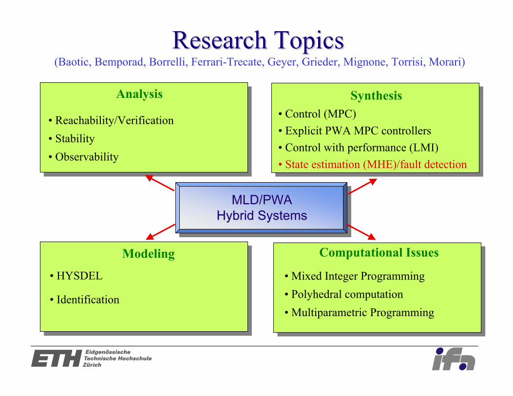
MLD/PWA MLD/PWA Hybrid SystemsHybrid Systems

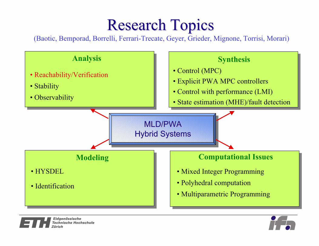
• Reachability/Verification• Stability• Observability

• HYSDEL

• Identification

Research TopicsResearch Topics

Analysis

Computational IssuesModeling

• Control (MPC)• Explicit PWA MPC controllers• Control with performance (LMI)• State estimation (MHE)/fault detection

Synthesis

• Mixed Integer Programming• Polyhedral computation• Multiparametric Programming

(Baotic, Bemporad, Borrelli, Ferrari-Trecate, Geyer, Grieder, Mignone, Torrisi, Morari)

ObservabilityObservability

The MLD system is observable in T steps on Uandif there exists a scalar w > 0 such that, ∀ u(t){ }Tà1

t=0

minP

t=0Tà1 y 1(t) à y 2(t)k k∞ à w x 1 ,0 à x 2 ,0k k1 õ 0

x 1 ,0 , x 2 ,0 ∈ X(0)w.r.t. and u(t) ∈ U and subj. to the MLDequations + constraints.

X(0)

Observability is undecidable(Sontag, 1996)

(Sontag, 1996)

Sets of admissible initial states and inputsX (0 ) U

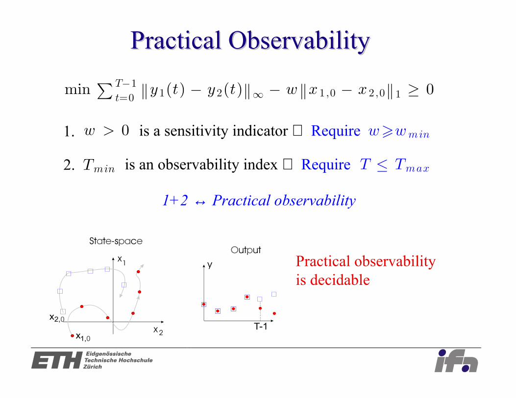
Practical ObservabilityPractical Observability

w > 0

minP

t=0Tà1 y 1(t) à y 2(t)k k∞ à w x 1 ,0 à x 2 ,0k k1 õ 0

Practical observability is decidable

1. is a sensitivity indicator ⇒ Require w>wmin

2. T ô Tmax

1+2 ↔ Practical observability

Tmin is an observability index ⇒ Require

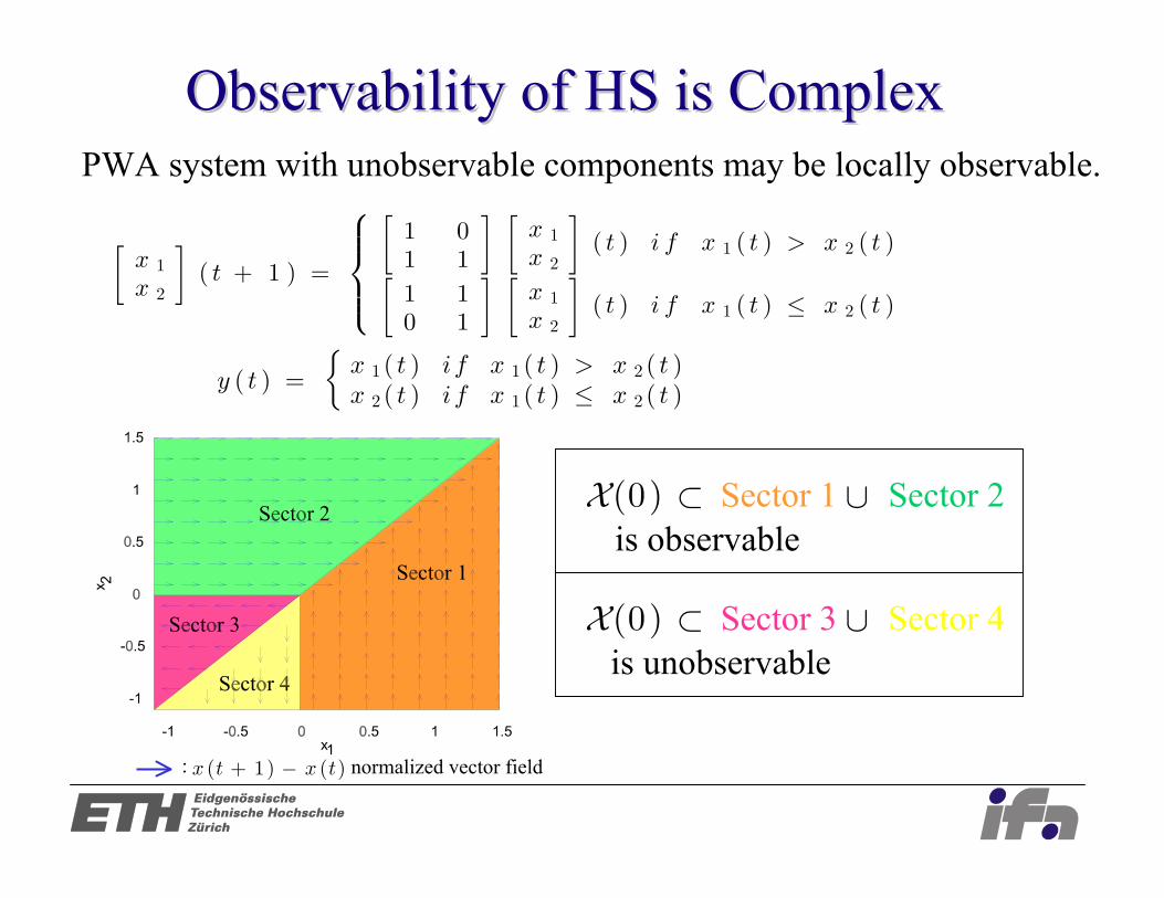
Observability Observability of HS is Complexof HS is ComplexPWA system with unobservable components may be locally observable.

x 1

x 2

ô õ( t + 1 ) =

1 01 1

ô õx 1

x 2

ô õ( t ) i f x 1 ( t ) > x 2 ( t )

1 10 1

ô õx 1

x 2

ô õ( t ) i f x 1 ( t ) ô x 2 ( t )

y ( t ) =

x 1 ( t ) i f x 1 ( t ) > x 2 ( t )x 2 ( t ) i f x 1 ( t ) ô x 2 ( t )

ú

: x (t + 1) à x (t) normalized vector field

X(0) ú Sector 1 ∪ Sector 2is observable

X(0) ú Sector 3 ∪ Sector 4is unobservable

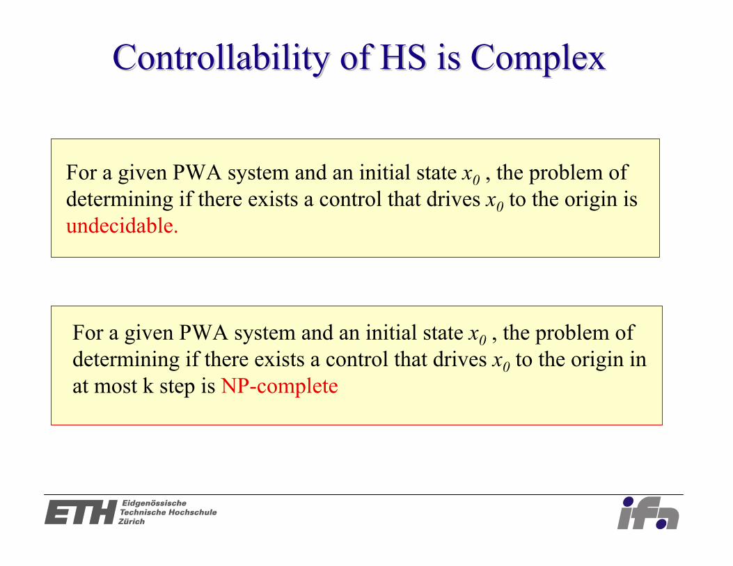
Controllability of HS is ComplexControllability of HS is Complex

For a given PWA system and an initial state x0 , the problem of determining if there exists a control that drives x0 to the origin is undecidable.

For a given PWA system and an initial state x0 , the problem of determining if there exists a control that drives x0 to the origin in at most k step is NP-complete



• HYSDEL

• Identification


Analysis



Synthesis



• Is reachable from in steps ?

• Target sets (disjoint)

• A hybrid system X(0)

Σ

ReachabilityReachability Analysis/VerificationAnalysis/Verification

• Given:

Z1, Z2, . . ., ZL

t ô Tmax• Problem: Zi X(0)X(0)

Zi

XZi(0)

XZi(0)

• A set of initial conditions

• Time horizon

• If yes, from which subset of ? • Disturbance/input sequences driving to .

Z1

Z2

ZL

XZ1(0)

XZ2(0)

XZL(0)

X(0)

Tmax

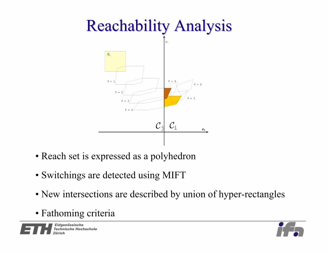
• Reach set is expressed as a polyhedron

• Switchings are detected using MIFT

• New intersections are described by union of hyper-rectangles

• Fathoming criteria

Reachability Reachability AnalysisAnalysisX0

t = 1

t = 2

t = 3

t = 4

x1

x2

t = 5

t = 6t = 4

x2x2Cj Ci

ApplicationsApplications• Safety ( = unsafe sets)Z1, Z2, . . ., ZL

• Stability ( = invariant set around the origin)Z1

• Scheduling

• Performance Assessment of Model Predictive Control( =invariant set around the origin, =set of infeasible states)Z1 Z2

Z1• Liveness ( =set to be reached within a finite time)

• Robust Simulation



• HYSDEL

• Identification


Analysis



Synthesis



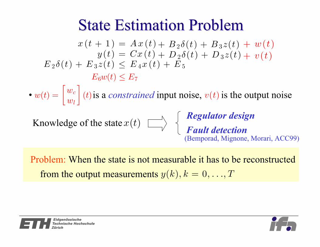
• is a constrained input noise, is the output noise

State Estimation ProblemState Estimation Problem

Knowledge of the stateRegulator designFault detection

Problem: When the state is not measurable it has to be reconstructed from the output measurements y(k), k = 0, . . ., T

x(t)

x (t + 1) = Ax (t)y (t) = Cx (t)

+ B 2î(t) + B 3z(t)+ D 2î(t) + D 3z(t)

E 2î(t) + E 3z(t) ô E 4x (t) + E 5

w(t) =wc

wl

ô õ(t) v(t)

+ w (t)+ v (t)

E6w(t) ô E7

(Bemporad, Mignone, Morari, ACC99)

Moving Horizon Estimation (MHE)Moving Horizon Estimation (MHE)

ΘãT =min

x(TàM),w

Pk=TàMTà1 kw(k)k2Q+kv(k)k2R+ΓTàM x(TàM)( )

Initial penalty (summarizing the neglected data)

(Michalska, Mayne, Morari, Muske, Rao, Rawlings ...)

: fixed time horizonM> 0

are available

Tà 1

y(TàM), . . ., y(Tà 1)

1) Solve

subj. to MLD dynamics + constraints

2) At time collect , shift the data window and cycle ...

and compute the estimates xê(TàM|T), . . ., xê(T|T)T y(T)

Time

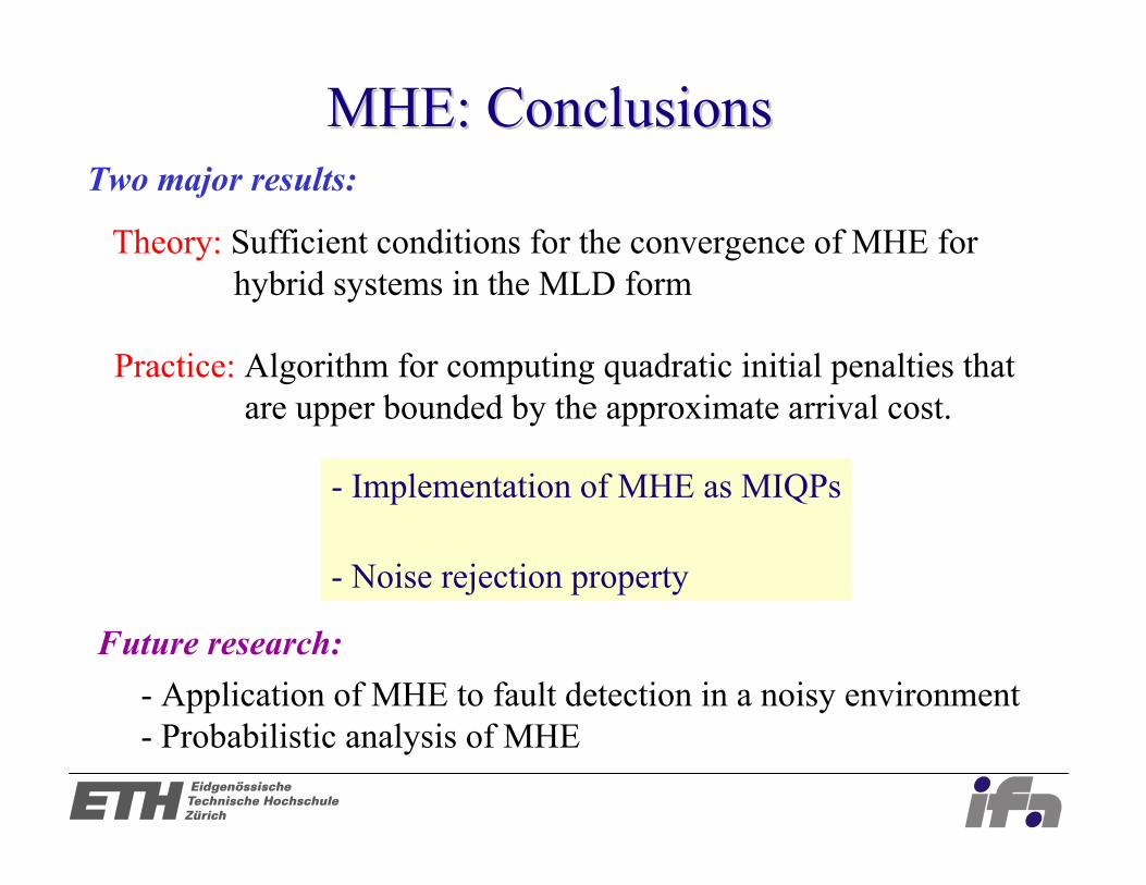
MHE: ConclusionsMHE: Conclusions

- Implementation of MHE as MIQPs

- Noise rejection property

Theory: Sufficient conditions for the convergence of MHE for hybrid systems in the MLD form

Practice: Algorithm for computing quadratic initial penalties that are upper bounded by the approximate arrival cost.

Two major results:

- Application of MHE to fault detection in a noisy environment- Probabilistic analysis of MHE

Future research:



• HYSDEL

• Identification


Analysis



Synthesis



IdentificationIdentification

• Model orders , fixedna nb

• models input/output constraints Examples:

Xë ô u (k) ô ì|y(k + 1) à y(k)| ô í

The shape of is knownX

The switching law is assumed unknown: Both the submodels and theshape of the regions must be estimated from the dataset

• The number of submodels is known s

Dataset: S = {(x(k), y(k)), k = 1, . . ., N}

If the regions are known the identification problem amounts to the identification of ARX models

Xis

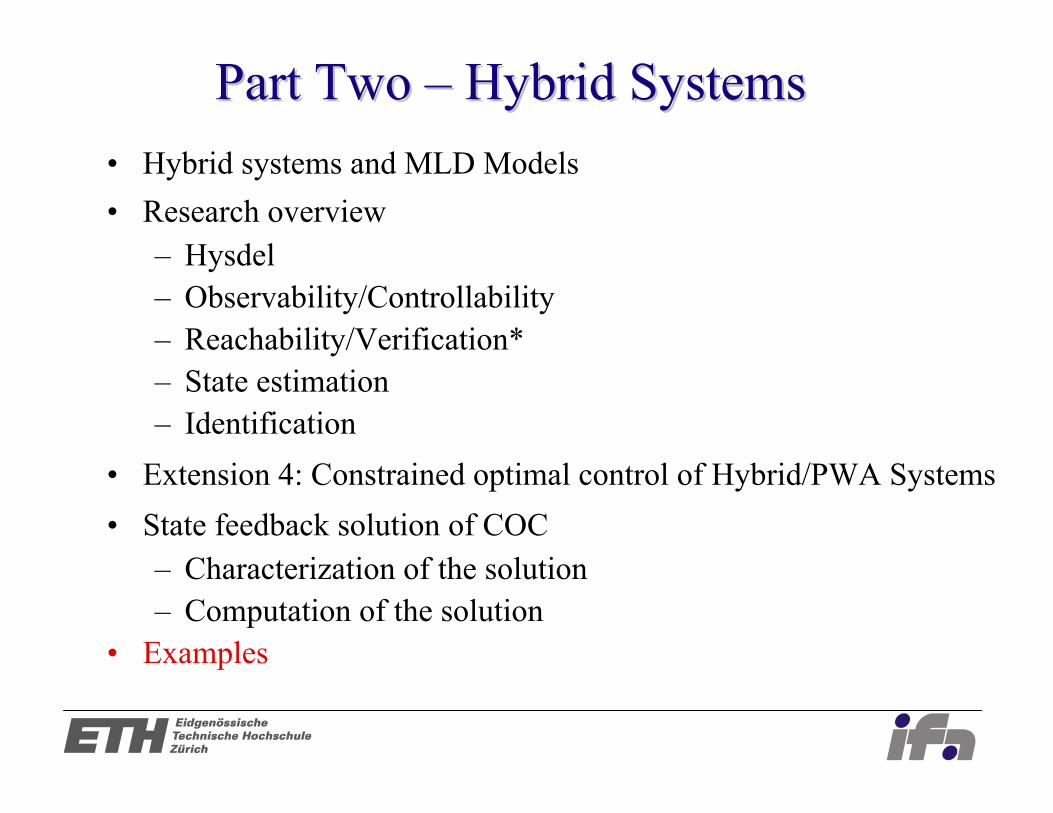
Part Two Part Two –– Hybrid SystemsHybrid Systems• Hybrid systems and MLD Models• Research overview

– Hysdel– Observability/Controllability– Reachability/Verification*– State estimation– Identification

• Extension 4: Constrained optimal control of Hybrid/PWA Systems• State feedback solution of COC

– Characterization of the solution – Computation of the solution

• Examples

Extension 4: Hybrid/PWA SystemsExtension 4: Hybrid/PWA Systemsmin

U||Px(N)||p + P

k=0

Nà1 ||Qx(k)||p + ||Ru(k)||p

x(k) ∈ Rn, u(k) ∈ Rm, U,{u(0), u(1), . . ., u(N à 1)}

subj.to x(t +1) = Aix(t) +Biu(t) + fiif [x(t), u(t)] ∈ Xi, i = 1, . . ., s

Ex(k) +Lu(k) ô M, k = 0, . . ., N à 1x(N) ∈ Xf

u*(0) is used in a Receding Horizon fashion for infinite time control

Feedback control law?

Translation into Mixed Integer ProgramTranslation into Mixed Integer Program

s.t. Gï ô w +Fx(0)

minï

ïTHï + (fT + x(0)TF)ï

subj. to

x(N) ∈ Xf

x(k + 1) = Ax(k) +B1u(k) +B2î(k) +B3z(k)y(k) = Cx(k) +D1u(k) +D2î(k) +D3z(k)

E2î(k) + E3z(k) ô E1u(k) + E4x(k) + E5

minUN

J(UN, x(0)), kPx(N)kp + Pk=0

Nà1kQx(k)kp + kRu(k)kp

Mixed Integer Program

Equivalent MLD representation of the PWA system

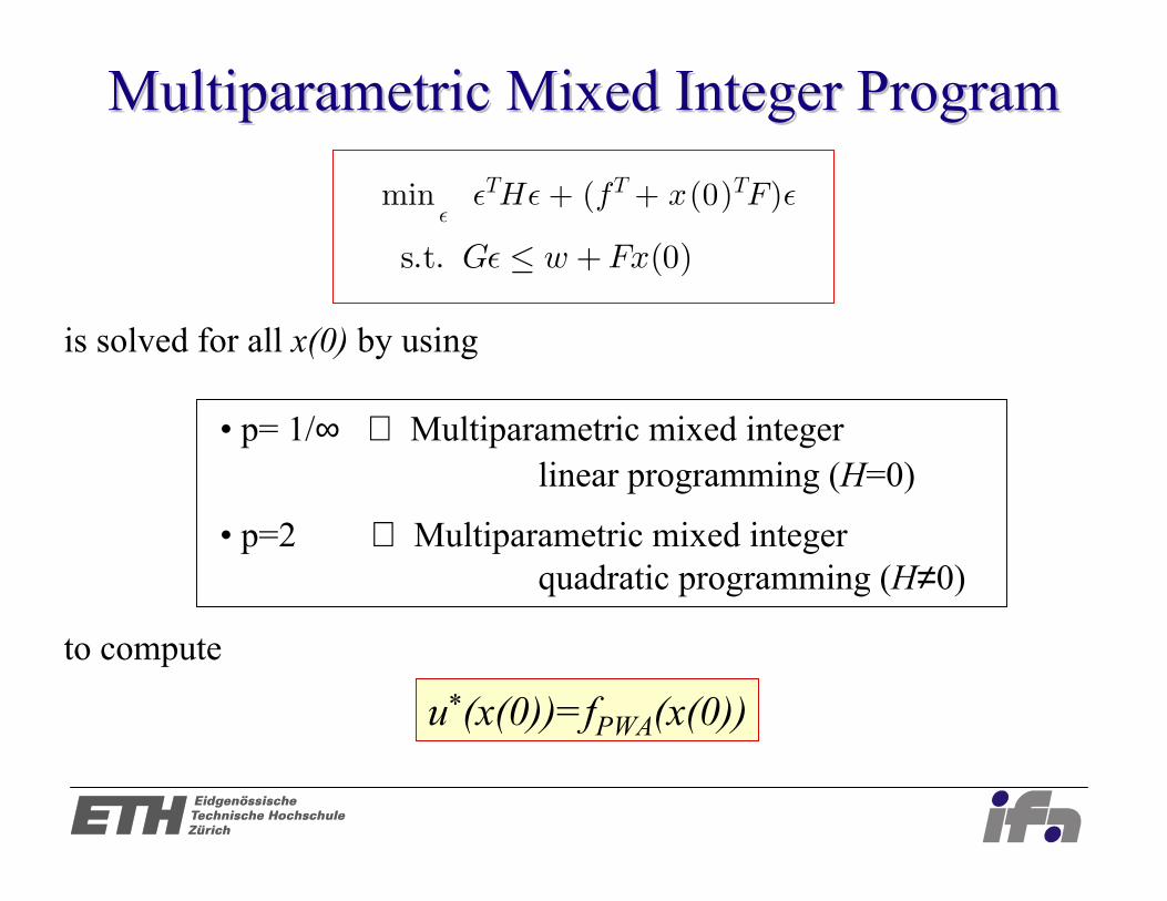
Multiparametric Mixed Integer ProgramMultiparametric Mixed Integer Program

is solved for all x(0) by using

• p= 1/∞ ⇒ Multiparametric mixed integerlinear programming (H=0)

• p=2 ⇒ Multiparametric mixed integer quadratic programming (H≠0)

s.t. Gï ô w +Fx(0)

minï

ïTHï + (fT + x(0)TF)ï

to compute

u*(x(0))=fPWA(x(0))





• Examples

Characterization of the Solution (p=2) Characterization of the Solution (p=2)

The solution to the optimal control problem is a time varying PWA state feedback control law of the form

partition of the set of feasible states x(k).{Pki}Nk

i=1

(Sontag 1981, Mayne 2001)

if x(k) ∈ Pki,{x : x0Lk

i(j)x +Mk

i(j)x ô Kk

i(j)}

uã(x(k)) = Fkix(k) +Gk

i

Xãk

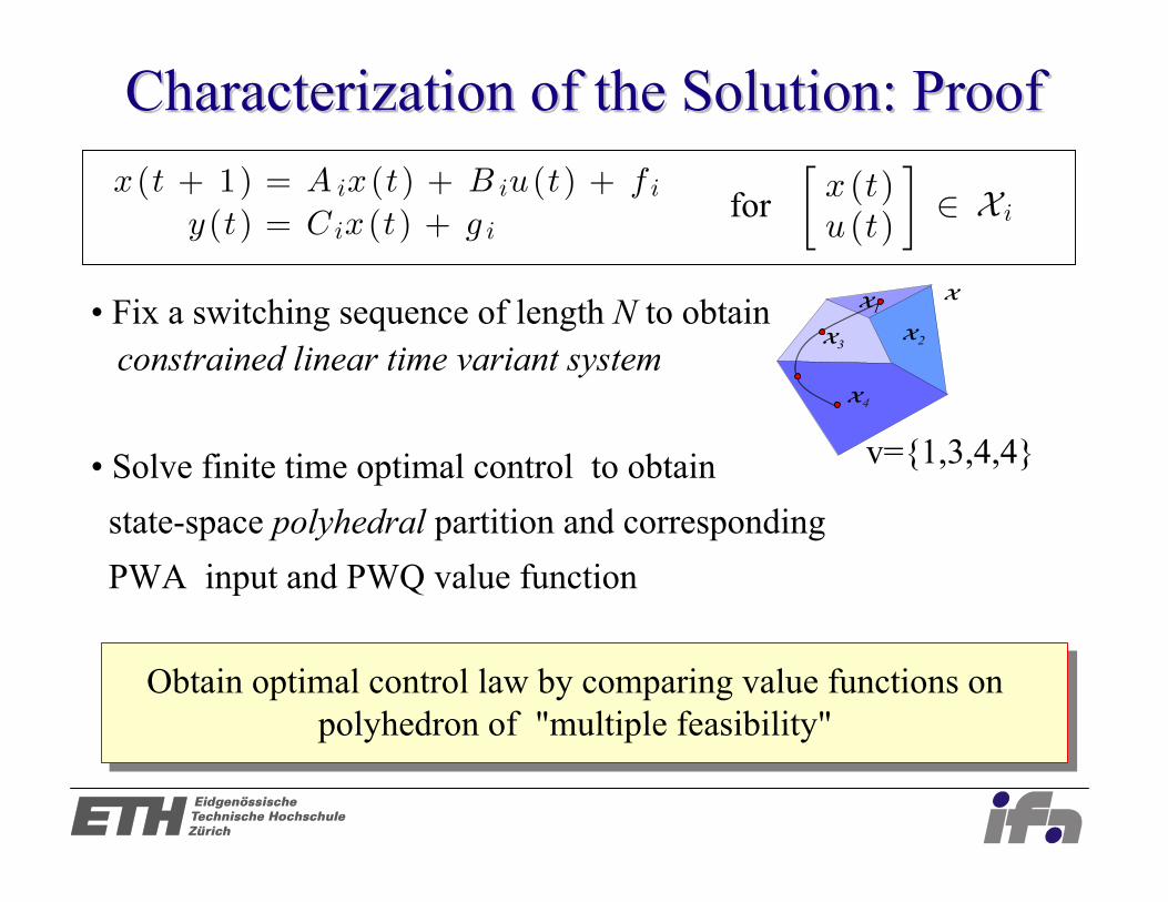
Characterization of the Solution: ProofCharacterization of the Solution: Proof

• Fix a switching sequence of length N to obtainconstrained linear time variant system

• Solve finite time optimal control to obtainstate-space polyhedral partition and correspondingPWA input and PWQ value function

v={1,3,4,4}

x(t + 1) = A ix(t) + B iu(t) + f i

y (t) = Cix(t) + g ifor x (t)

u (t)

ô õ∈ X i

Obtain optimal control law by comparing value functions on polyhedron of "multiple feasibility"

v1={1,2,3,4}

v2={1,2,3,3}

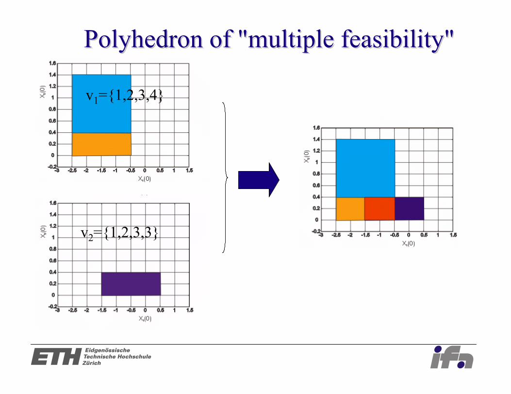
Polyhedron of "multiple feasibility"Polyhedron of "multiple feasibility"

v1={1,2,3,4}

v2={1,2,3,3}

Polyhedron of multiple feasibility:switch v1 and v2 both admissible


v1={1,2,3,4}

v2={1,2,3,3}


v1={1,2,3,4}

v2={1,2,3,3}

1

2 3 4 5


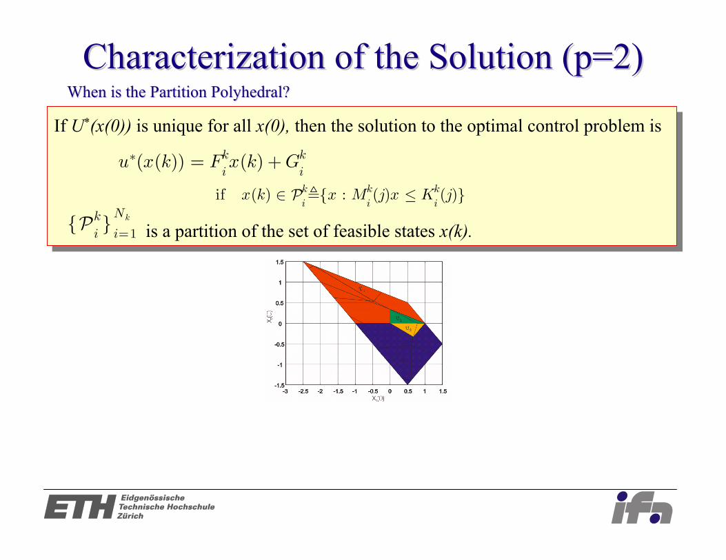
If U*(x(0)) is unique for all x(0), then the solution to the optimal control problem is

is a partition of the set of feasible states x(k).

If U*(x(0)) is unique for all x(0), then the solution to the optimal control problem is

is a partition of the set of feasible states x(k).

When is the Partition Polyhedral?When is the Partition Polyhedral?

{Pki}Nk

i=1

Characterization of the Solution (p=2) Characterization of the Solution (p=2)

if x(k) ∈ Pki,{x : Mk

i(j)x ô Kk

i(j)}


i

Polyhedral Partition: ProofPolyhedral Partition: Proof

Continuity of the PWA optimal control law excludes Case 3

• Possible intersections of the value functions

Case 1 Case 2 Case 3

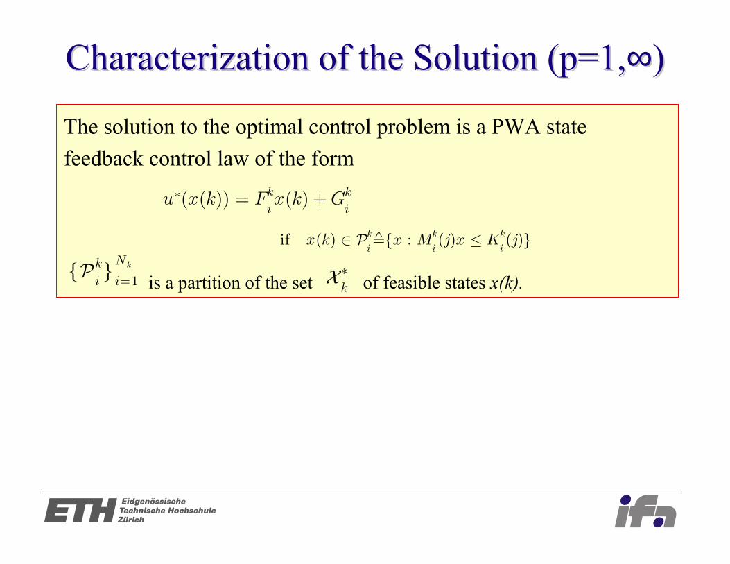
Characterization of the Solution (p=1,Characterization of the Solution (p=1,∞∞))

The solution to the optimal control problem is a PWA state feedback control law of the form

is a partition of the set of feasible states x(k).{Pki}Nk

i=1


i

if x(k) ∈ Pki,{x : Mk

i(j)x ô Kk

i(j)}

Xãk





• Examples

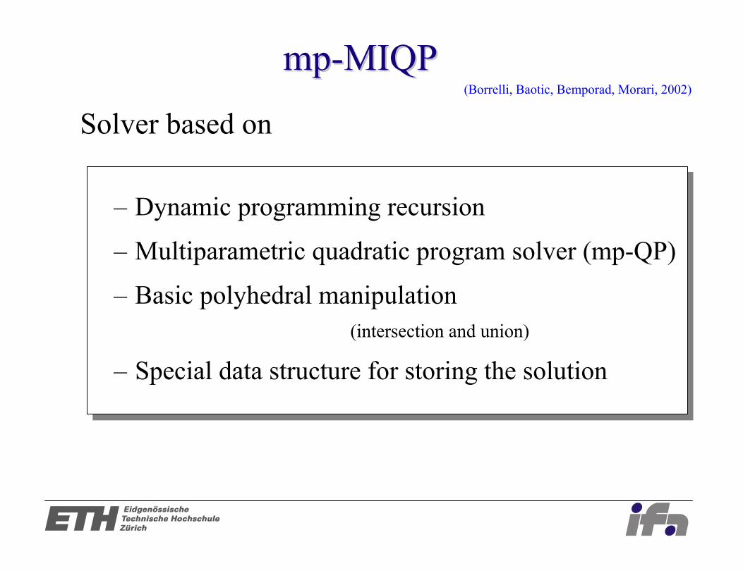
mpmp--MIQPMIQP

Solver based on

– Dynamic programming recursion

– Multiparametric quadratic program solver (mp-QP)

– Basic polyhedral manipulation (intersection and union)

– Special data structure for storing the solution

(Borrelli, Baotic, Bemporad, Morari, 2002)

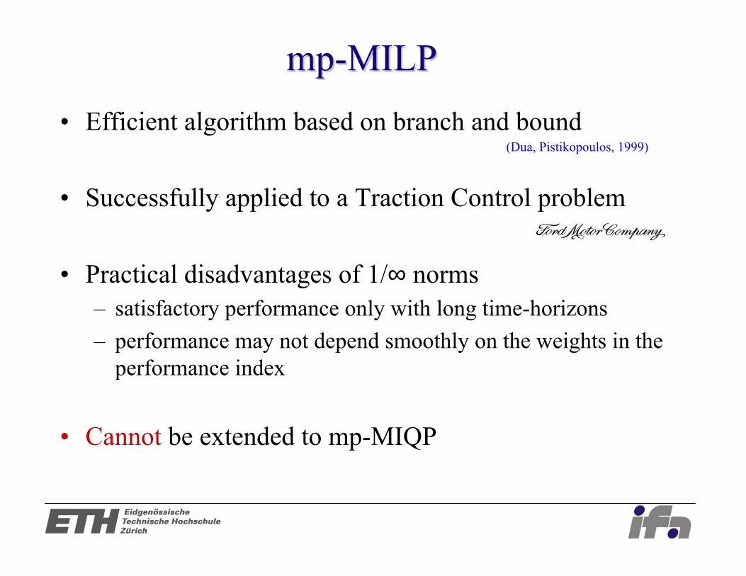
mpmp--MILPMILP• Efficient algorithm based on branch and bound

• Successfully applied to a Traction Control problem

• Practical disadvantages of 1/∞ norms– satisfactory performance only with long time-horizons– performance may not depend smoothly on the weights in the

performance index

• Cannot be extended to mp-MIQP

(Dua, Pistikopoulos, 1999)

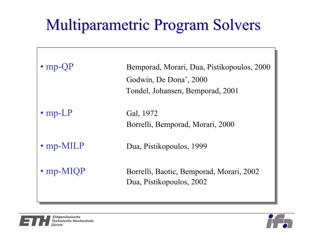
• mp-QP Bemporad, Morari, Dua, Pistikopoulos, 2000 Godwin, De Dona’, 2000 Tondel, Johansen, Bemporad, 2001

• mp-LP Gal, 1972Borrelli, Bemporad, Morari, 2000

• mp-MILP Dua, Pistikopoulos, 1999

• mp-MIQP Borrelli, Baotic, Bemporad, Morari, 2002Dua, Pistikopoulos, 2002

• mp-QP Bemporad, Morari, Dua, Pistikopoulos, 2000 Godwin, De Dona’, 2000 Tondel, Johansen, Bemporad, 2001

• mp-LP Gal, 1972Borrelli, Bemporad, Morari, 2000

• mp-MILP Dua, Pistikopoulos, 1999

• mp-MIQP Borrelli, Baotic, Bemporad, Morari, 2002Dua, Pistikopoulos, 2002

Multiparametric Program SolversMultiparametric Program Solvers

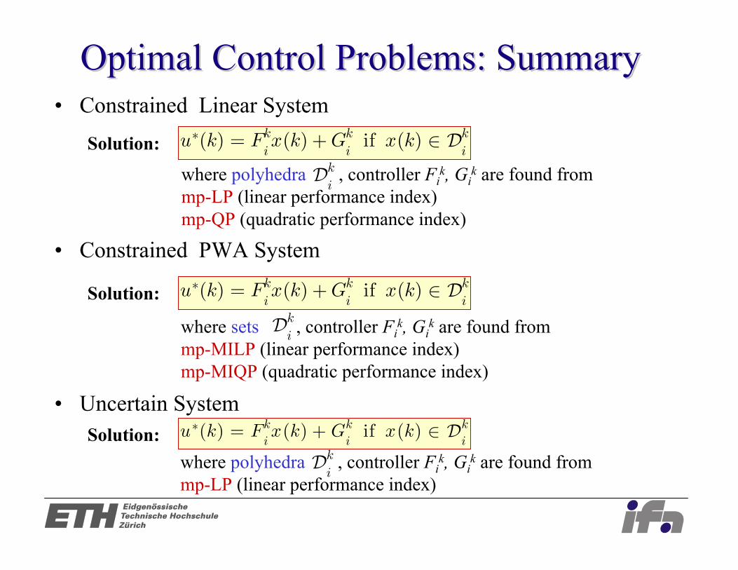
Optimal Control Problems: SummaryOptimal Control Problems: Summary• Constrained Linear System

• Constrained PWA System

• Uncertain System

uã(k) = Fkix(k) +Gk

iif x(k) ∈ Dk

iSolution:where polyhedra , controller Fi

k, Gik are found from

mp-LP (linear performance index)mp-QP (quadratic performance index)

Dki

uã(k) = Fkix(k) +Gk

iif x(k) ∈ Dk

iSolution:

where sets , controller Fik, Gi

k are found from mp-MILP (linear performance index)mp-MIQP (quadratic performance index)

Dki

uã(k) = Fkix(k) + Gk

iif x(k) ∈ Dk

iSolution:where polyhedra , controller Fi

k, Gik are found from

mp-LP (linear performance index)Dk

i





• Examples

• Traction control (Ford Research Center )

• Gas supply system (Kawasaki Steel )• Batch evaporator system (Esprit Project 26270 )• Anesthesia (Hospital Bern )• Hydroelectric power plant ( )• Power generation scheduling ( )

• Integrated management of the power-train ( )

• Gear shift operation on automotive vehicles ( )

ApplicationsApplications

Simple ExampleSimple Example

Furnaces

Amount of heating power is constant

(Hedlund and Rantzer, CDC1999)

Bi =

10

ô õif first furnace heated

01

ô õif second furnace heated

00

ô õif no heating

• Objective: • Control the temperature

to a given set-point

• Constraints:• Only three operation modes:

1- Heat only the first furnace2- Heat only the second furnace3- Do not heat any furnaces

Tç1Tç2

ô õ= à 1 0

0 à 2

ô õT1

T2

ô õ+Biu0

T1, T2

u0

Alternate Heating of Two FurnacesAlternate Heating of Two Furnaces

• MLD system

• mp-MILP optimization problem

to be solved in the region

• Computational complexity of mp-MILP

minv2

0

n o J(v20, x(t)),P

k=02 kR(v(k + 1)à v(k))k∞+ kQ(x(k|t)à xe)k∞

u(t) =1 0 0[ ] if first furnace heated0 1 0[ ] if second furnace heated0 0 1[ ] if no heating

State x(t) 2 variables

Input u(t) 3 variables

Aux. binary vector δ(t) 0 variables

Aux. continuous vector z(t) 9 variables

à 1 ô x1 ô 1à 1 ô x2 ô 10 ô u0 ô 1

linear constraints 168

continuous variables 33

binary variables 9

parameters 3

time to solve the mp-MILP 5 min

number of regions 105

Sampling time = 0.08 s

Alternate Heating of Two FurnacesAlternate Heating of Two Furnaces

parameterized !

T1

T2

Heat 2

No Heat

mpmp--MILP SolutionMILP Solutionu0=0.8

T1

T2

Heat 1

Heat 2

No Heat

X1

X2

X1

X2

u0=0.4

Set point cannot be reached Set point is reached

Heat 1

ExampleExample

Traction Control

Hybrid Control Design for Traction Hybrid Control Design for Traction ControlControl

• Francesco Borrelli • Alberto Bemporad• Manfred Morari

• Mike Fodor• Davor Hrovat• Mitch McConnell

research topics - aem - aerospace engineering and ... a given pwa system and an initial state x0,...

Documents