Copenhagen  Business  School  

Research  on  Stock  Index  Futures  -­‐-­‐-­‐An  empirical  analysis  of  CSI  300  stock  index  futures  

Lu  Zhang  (luzh11ab@student.cbs.dk)  

MASTER  THESIS    Supervisor:  Lars  Sønnich  Pørksen      Cand.merc  Finance  and  Strategic  Management  Copenhagen  Business  School  2014    No.  of  Pages:  70  No.  of  Characters:  131,353  Date:  20.05.2014      

1

Acknowledgement

I would like to express my sincere appreciation to my supervisor Lars Sønnich

Pørksen for all the invaluable suggestions, professional guidance and kind

encouragement. Also, I like to thank my parents and my husband for their love and

constant support.

2

Abstract With the fast expanding of stock market scale in China, the number of investors is

growing, and the methods for better risk management are eagerly required. Moreover,

CSI 300 stock index futures contract was first listed on China Financial Futures

Exchange on April 16, 2010, which attached more and more attention of domestic and

overseas investors. It ended the time period of China’s unilateral capital market.

Also as we know, stock index futures hedging can be utilized by investors to manage

the system risk in their investment portfolio, which will provide the reference for

investors to plan their investment. The key of hedging implementation is the hedge

ratio defining. Therefore, the research problems of this thesis are whether the

launching of CSI 300 stock index futures can effectively play a hedging role and how

it hedges. Based on the related theories of the stock index futures and hedging, the

CSI 300 stock index futures hedging effect will be analyzed and estimated in the

process of empirical research.

First of all, in order to understand the related economic knowledge, the definitions of

stock index futures are described, the relevant economic functions are introduced, and

the hedge theories are reviewed; which provides an essential theoretical basis for the

empirical study. Furthermore, the development of China’s stock market and its index

futures market are also reviewed, and the comparison between CSI 300 index futures

contracts and other different index futures with a China concept are subsequently

conducted, which confirms the necessity of this research.

Then, the correlation between CSI 300 stock index futures and spot index are

analyzed. According to their closing price, their returns are calculated. Based on these

data, the descriptive statistics test, the ADF test and the cointegration test are

conducted to verify the relevance of CSI 300 stock index spot and futures markets,

and insure there exists a long-term stability cointegration relationship between them,

which is a preparation for the further empirical studies.

For the purpose of estimating the optimal hedge ratio, and evaluating the hedging

effect from the point of view of returns and variance, the methods of OLS model and

GARCH model are applied based on actual market data, and comparative analysis is

utilized to analyze the hedging effect of CSI 300 stock index futures and H-shares

index futures. Overall, it can be shown that the launch of CSI 300 stock index futures

indeed played an effective hedging role to avoid the systemic risk in the stock market.

3

Table of Contents

Acknowledgement  ..................................................................................................  1  

Abstract  ..................................................................................................................  2  

1   Introduction  ......................................................................................................  5  1.1   Background  .................................................................................................................................................  5  1.2   Research motivation  .................................................................................................................................  7  

1.2.1   Theoretical significance  ....................................................................................................................  7  1.2.2   Practical significance  ........................................................................................................................  7  

1.3   Literature Review  ......................................................................................................................................  7  1.3.1   Stock index futures  ..............................................................................................................................  7  1.3.2   Hedging  ...................................................................................................................................................  8  

1.4   Problem statement  ..................................................................................................................................  10  1.5   Methodology  ............................................................................................................................................  11  1.6   Delimitations  ............................................................................................................................................  11  

2   Stock  index  futures  and  hedging  .....................................................................  13  2.1   Related theory of stock index futures  ..............................................................................................  13  

2.1.1   Concept  .................................................................................................................................................  13  2.1.2   Characteristics  ...................................................................................................................................  13  2.1.3   Functions  ..............................................................................................................................................  16  

2.2   Related theory of hedging  ...................................................................................................................  18  2.2.1   Concept  .................................................................................................................................................  18  2.2.2   Economic principles  ........................................................................................................................  19  2.2.3   Types  ......................................................................................................................................................  20  2.2.4   The Basis Theory  ..............................................................................................................................  21  2.2.5   The hedging theory  ...........................................................................................................................  23  

3   Development  of  stock  index  futures  in  China  ..................................................  26  3.1   Development of stock market in China  ..........................................................................................  26  

3.1.1   Chinese stock market  .......................................................................................................................  26  3.1.2   Reform of Chinese stock market  .................................................................................................  27  

3.2   Development of CSI 300 index futures  ..........................................................................................  29  3.2.1   Significance of CSI 300 index futures  .......................................................................................  30  

3.3   CSI 300 Index and CSI 300 stock index futures  ..........................................................................  31  3.3.1   Pricing CSI 300 Index  .....................................................................................................................  31  3.3.2   Relation with Shanghai index and Shenzhen index  .............................................................  31  3.3.3   Comparing with other Chinese concept stock index futures  ............................................  32  3.3.4   Comparing CSI 300 index futures contract with H-shares index futures contract  .  35  

4   The  general  principle  of  the  determination  of  optimal  hedge  ratio  ..................  37  4.1   Estimation models of optimal hedge ratio  .....................................................................................  37  

4.1.1   Risk minimizing hedging model  ..................................................................................................  37  4.1.2   Utility maximizing hedging model  .............................................................................................  38  4.1.3   Per unit risk compensation maximization  ...............................................................................  38  

4.2   Estimating hedging effectiveness based on risk-minimization hedging model  .................  39  4.2.1   Econometric models for hedging  ................................................................................................  39  4.2.2   Estimating Hedging Effectiveness  ..............................................................................................  40  

5   Empirical  analysis  ............................................................................................  42  5.1   Data collection and processing  ..........................................................................................................  42  5.2   Data analysis  ............................................................................................................................................  43  

5.2.1   Descriptive statistics analysis  ......................................................................................................  43  5.2.2   Stationary test  ....................................................................................................................................  46  

4

5.2.3   Cointegration test  .............................................................................................................................  47  5.2.4   Summary  ...............................................................................................................................................  49  

5.3   Hedging Model Analysis  .....................................................................................................................  49  5.3.1   OLS Model  ...........................................................................................................................................  50  5.3.2   GARCH Model  ...................................................................................................................................  52  

5.4   Hedging effectiveness analysis  ..........................................................................................................  54  6   Conclusion  and  perspective  .............................................................................  57  6.1   Conclusion  ................................................................................................................................................  57  6.2   Suggestions for investors  .....................................................................................................................  58  6.3   Limitations and future work  ...............................................................................................................  59  

Reference  .............................................................................................................  61  

Appendix  ..............................................................................................................  64  

5

1 Introduction

1.1 Background From July 2007, the financial crisis, which was triggered by the U.S. subprime

mortgage crisis, has spread out to the surrounding countries and eventually became

the global financial crisis. Because of the global financial turmoil, the systemic risk of

the capital market is further increased. The investors need a financial tool to avoid the

risk and fix the future cost and profit. By using financial derivatives, it is a good

choice for investors to hedge.

As a common financial instrument, the stock index futures were born in U.S. In

February 1982, stock index futures was firstly created by KCBT (Kansas city board of

trade), which was named as value line index future. Two months later, the Chicago

Board of Trade started trading the S&P stock index futures contracts (Robert, 2006).

The introduction of stock index futures in the U.S activated the financial markets, and

expanded the size of the U.S. domestic futures market. Following the U.S., Australia,

Britain, Canada, Japan, Singapore, Hong Kong and other countries or regions have

launched their stock index futures (Zhang, 2011). In recent years, with the continuous

development of the world economy, trading varieties of the stock index futures are

increasing and the transaction scope is expanding. Nowadays, stock index futures play

a more and more important role in the financial derivatives market.

In China, the commodity futures trading (including gold, soybeans, crude oil and etc)

has started for many years. However, the introduction of stock index futures has a

special significance for China, because it is a first financial futures launched in China

since the mid 1990s1. Along with the appearance of some economic problems (such as

the RMB appreciation, the inflationary pressures, the pressure of capital inflow and so

on), many uncertainties will affect the Chinese economic development, especially the

risk impact in capital market (Chen & Li, 2013). With the growth and development of

institutional investors in China, the demands of using stock index futures to manage

the risk of investment portfolio are growing. Before the launching of CSI 300 stock

index futures, investors can only trade in Hong Kong index futures market to reduce

their risk. It took China about four years to promote the CSI300 Stock Index Futures.

1 http://www.ftchinese.com/story/001032240/en

6

Finally, it came out on April 16th, 2010 and traded in the China Financial Futures

Exchange2.

The official trading of CSI300 stock index futures, it provides investors a new

investment instrument and a hedging tool, which enriches financial products in the

futures market, and connects the securities and futures markets; also it brings the

changes in market transactions and trading concepts, which leads to complexity of the

investment strategies and diversity of products. Moreover, the official trading of

CSI300 stock index futures brings investors become more specialized and

institutional.

Since CSI 300 stock index futures were brought into operation in 2010, the opening of

futures customer accounts has a steady growth and the trading is active. That is

because the futures price normally match the spot price with a high degree and it

shows a good control of market risk. Also among the contract months, the most

actively traded futures contracts are current month, therefore the futures contracts

show a good momentum of development.

On February 3rd, 2012, the China Financial Futures Exchange issued “the

Administrative Measures of the China Financial Futures Exchange for Hedging and

Arbitrage Trading” (revised)3. Not only it gave advices to further optimize the

management of hedging, but also it introduced the systems and measures of arbitrage,

which would be helpful for introducing institutional investors and sophisticated

individual investors. However, the Chinese stock index futures started later than other

countries, and the investors lacked the knowledge of its function, so many related

things are at the exploratory stage. We can expect that only if the stock futures market

performs its risk avert function fully, it can meet the requirements of investors for

hedging and arbitrage, thus avoid the risk of stock market effectively.

Based on the above background related to the development of China’s stock index

futures market, this thesis will give a quantitative and qualitative analysis on the

hedging performance of CSI300 stock index futures by using the futures trading data

in almost four years, which are the main research subjects.

2 http://www.ft.com/intl/cms/s/0/5e907942-48ef-11df-8af4-00144feab49a.html#axzz31oRZvZtm 3 http://www.lawinfochina.com/display.aspx?lib=law&id=10707&CGid=

7

1.2 Research motivation

1.2.1 Theoretical significance

This study combines the theories about the stock index futures and hedging with the

volatility characteristics of China’s securities market; also econometric models will be

adopted as tools to analyze the functions of hedging in a quantitative way. The aim is

to further explore the front problem of risk management in stock portfolio investment

and promote the improvement of the theoretical system of stock index futures.

1.2.2 Practical significance

In the capital market, risk is everywhere. Although it cannot be eliminated

fundamentally, it can be reduced by efficient investment. For investors, it is very

important to reach the goal of avoiding risk and locking returns in capital market.

Based on the developing actuality of Chinese stock index futures and the analysis of

the relevance between stock index futures and spot index, this paper estimates the

effect of hedging and aims to provide an effective risk management tool for investors,

which can help them allocate the assets rationally within the scope of risk control and

enhance the efficiency of investment.

1.3 Literature Review

1.3.1 Stock index futures

Edwards (1988) examined the volatility of the stock market both before and after the

start of futures trading through the empirical analysis of S&P500 index. The result

shows that the introduction of futures trading does not cause the increment in stock

price volatility. On the contrary, the introduction of stock index futures contracts has

improved the financial market, which makes the stock market more stable.

Harris (1989) studied on S&P500 stock index futures. Through empirical analysis, the

research expresses that there is a great volatility in stock index futures market. One

reason is the illiquidity of the corresponding market due to the large volume of trade

in a short time and another reason is that the existence of stock futures market speeds

up the flow of information, which accelerate the main constituent stocks’ reaction of

new information consequently.

In the study of Bessembinder and Seguin (1992), the situations before and after the

introduction of S&P500 index futures from 1978 to 1989 were analyzed and

8

compared. It can be found out that the introduction of futures market does not

increase the volatility of the spot market, but makes volatility decline in the spot

market.

Lee and Ohk (1992) studied the relationship between the Hang Seng Index and its

futures from 1984 to 1988. They thought that the introduction of Hang Seng stock

index futures had reduced volatility of the spot market.

In order to test the impact of stock index futures on the volatility of the spot market,

Mayhew (2000) used data from 25 countries (that had launched stock index futures)

to do empirical research. Through his study, it can be found that only in a few

countries, the volatility of the stock market may be relevant to the introduction of

stock index futures; and in most of the others, the relevance is not significant.

Salil K. Sarkar (2002) did a research on the development of stock index futures

contracts. He supposed that the fast development of the contracts is partly because

that investors want to avoid risk in portfolios.

1.3.2 Hedging

The most important function of futures trading is hedging. In the process of hedging,

the main problem is to determine the number of required stock index futures

contracts. And for calculating the number of contracts, the key issue is the

determination of hedge ratio.

Keynes (1951) and Hicks (1952) have firstly made a detailed exposition of traditional

hedge from the view of economics. It is believed that instead of getting high profits

from futures trading, the hedging aims to set off gains in one market against losses in

another market (hedge ratio is assumed as 1).

However, since traditional hedging theory deviates from the actual market situation, it

is found that the traditional hedge cannot completely reduce the systemic risk caused

by the stock price volatility. Therefore, many researchers have proposed the methods

using portfolio approach to estimate the optimal hedge ratio.

Under the condition of the minimum variance of the rate of return, Johnson (1960)

firstly proposed the concept of optimal hedge ratio of commodity futures, ordinary

least square regression (OLS) method and the formula for the optimal hedge ratio

calculation. With the assumption of constant volatility, the MV (minimum variance)

hedge ratio can be estimated using OLS.

9

Since Johnson (1960) proposed very early to explain hedging effect by Markowitz’s

portfolio theory, it made the hedging effectiveness issue become the core issue in the

research of futures market. On the basis of Johnson’s research, Ederington (1979)

applied the portfolio theory to the financial futures market, using OLS model to

analyze the hedge ratio of U.S. Treasury bond futures. The results indicated that the

hedge ratio was always less than 1, and the effect of risk aversion was better than the

situation when hedge ratio was 1. Besides, he gave the indicators of hedging

effectiveness of futures market, which reflected the decline level of risk after hedging.

In the classic capital market theory, it assumes that the variance of the returns is

constant. But a large amount of practical data analysis shows that there is a Volatility

Cluster of the returns. This characteristic would lead to heteroscedasticity. The

existence of heteroscedasticity makes the covariance (between spot and futures prices)

to be a variation. So the calculated hedge ratio is not constant, then the concept of

dynamic hedging is put forward.

Engle brought forward the autoregressive conditional heteroscedasticity model

(ARCH) in 1982. This model can capture the agglomeration effects of financial time

series. The representation and development of ARCH model provide a theoretical

basis and research method to estimate the dynamic hedge ratio. However, there are

too many lags in the regression, which too many parameters are required to be

estimated. That is why can the efficiency and accuracy of the estimation results are

affected.

Subsequently, Bollerslev (1986) developed GARCH model4. This model is a good

solution for the situation of excessive parameters to be estimated in ARCH model.

Cecchetti et at (1988), Kroner, Sulmn (1993), Park, Switzer (1995) and Gagnon,

Lypny (1995) have found that the dynamic hedge ratio was better than the constant

hedge ratio, and suggested traders should always adjust their positions to reduce their

risk exposure. In the research of Park and Switzer (1995), it found out that the using

of GARCH model improved hedging effectiveness over the OLS model.

However, Holmes (1995) used the data of FTSE-100 stock index futures from June

1984 to June 1992. By comparing the hedging effects of the traditional OLS, ECM

(error correction model) and the GARCH model, the result showed that the effect of

the OLS model was better than the other models. During the analysis on the hedging

4 GARCH model is the ARCH model as generalized autoregressive conditional heteroscedasticity.

10

performance, different researchers have obtained very different results by using

various models.

Over time, the researchers also found that using simple linear regression models to

estimate the hedging effectiveness, and ignoring cointegration relationship between

spot and futures prices, would reduce the hedging effect. Thus, they began to study

the long-term equilibrium relationship between futures and spot prices.

Wahab, Lashgari (1993) and Lien, Luo (1994) conducted further studies of the co-

integration relationship between stock index and futures market; and concluded that

when different models were applied to estimate the hedging performance, the co-

integration relationship should be considered.

The study of Lien (1996) summarized the impact of the co-integration relationship on

the hedging performance. He pointed out that if the co-integration relationship during

the estimation of hedge ratio was not considered, it would greatly reduce the hedging

effectiveness; and when evaluating the hedging effectiveness, the effect of using

GARCH model would be the best. Lien et al (2002) also proposed an indicator of

hedging performance. This indicator was expressed by the rate of change of returns’

variances before and after hedging. It was conducive to compare the hedge

effectiveness estimated by different models.

Though, the literatures have been reviewed are not newly findings. However, the

theories and models are already well established. The results of those researches are

practical and time tested, which can be adopted to study and analyze the newly

launched CSI 300 stock index futures in China.

1.4 Problem statement 1) What are the basic definitions of stock index futures and hedging? The related

theories and knowledge will be briefly introduced.

2) How is the development of stock index futures in China? What are CSI 300

Index and CSI 300 index futures? In this part, the development process of

stock index futures in China will be summarized and analyzed. And the

comparison between CSI 300 index futures and other index futures with China

concept will be presented.

3) What models can be used to obtain the optimal hedge ratio? How to estimate

the hedging effectiveness? The hedge ratio and hedging effectiveness of stock

index futures will be chosen as the evaluation indicators for hedging

11

performance, and the correlative models (OLS and GARCH) will be built to

estimate the indicators.

4) How is the correlation between CSI300 index futures market and the spot

market? Here, the correlation between the CSI300 index and the futures price

will be investigated, and the long-term equilibrium relationship between the

futures price and spot price will be discussed.

5) Based on the empirical analysis, how is the hedging performance of CSI 300

index futures compared with other index futures? In the professional

econometric software-Eviews, the OLS and the GARCH models will be used

to calculate the hedge ratio and the hedging effectiveness, and do a

comparative analysis with the calculation results.

1.5 Methodology

• Literature study

This paper studies a broad range of economic and financial literature in order to fully

understand the research focus, contents and relevant theoretical knowledge to

guarantee the smooth implementation of the research.

• Empirical study

This paper makes empirical research of hedging of the CSI300 index futures. Through

the relevant statistical test and regression analysis, it gives a reasonable evaluation on

the hedging performance of CSI300 index futures. In the meantime, it provides some

suggestions for hedgers, in order to fully reflect the practical value of this paper.

Statistical test: Using the ADF (augmented Dickey-Fuller) test and co-integration

test, the empirical analysis of the correlation between CSI 300 spot price and CSI 300

index futures price will be conducted. According to equations, the long-term

equilibrium relationship between the index and the CSI 300 index futures will be

studied.

Regression analysis: Using the OLS and GARCH models to calculate the

evaluation indicators of hedging performance of CSI300 index futures, the calculation

results will be compared and analyzed.

1.6 Delimitations The research data, which is used in this paper is daily closing price of CSI 300 index

futures, is lack of specific analysis of daily high frequency data. The study is not

12

focused enough at a micro-level. During the research process, in order to reflect the

continuity of the study period, we assume investors continually choose current month

contract to roll over. However, in reality, investors often use a hedging period from 30

days to 60 days. Also this study ignores the dynamic adjustment of hedging and the

required margin. In the process of empirical analysis, it is also ignored that the risk

preferences of different investors will be different. So there leaves some room for

further improvement.

13

2 Stock index futures and hedging

2.1 Related theory of stock index futures

2.1.1 Concept

Technically, stock index futures are the agreements to buy or sell a standardized value

of a stock index at a specified price on a future date. The trade object is the stock

index, using the changes of stock index as the standard. Stock index futures are settled

in cash and not by delivery of the underlying stocks (Hull, 2011). Also, they are

special kind of futures contracts by tracking the value of an underlying index. Stock

index is a comprehensive reflection of the market dynamics, which is used to analyze

and predict future movements of stock price for investors, or to provide the basis for

investment decisions. It tracks the changes of a portfolio of stocks (Hull, 2011). There

are three different ways to construct the stock market index, including price-weighted

index, value-weighted averages and the value line index. The value line index is an

equal-weighted arithmetic average.

Although the trading history of stock index futures is very short, they still have great

influence in the stock market. Stock index futures are important institutional

arrangements in the financial system to avoid market risks; also they are the most

important part in the financial derivatives market and cannot be replaced (Dubofsky &

Miller 2003). The essence of stock index futures is a process that investors transfer

the expected risk of the stock market price index to the futures market. This risk is

through buying or selling to cancel out each other when the investors have different

judgments on stock market curves. Like other futures (such as currency futures,

interest rate futures and other commodity futures), stock index futures are designed to

meet the needs of risk-aversion, and specifically designed to manage the price risk in

stock market.

2.1.2 Characteristics

Stock index futures are based on stock price index, which is the underlying asset of

the financial futures contracts. So it not only has the stock characteristics, but also has

the characteristics of futures and the specific features of its own.

14

2.1.2.1 Stock characteristics (Kolb, 2003)

From the viewpoint of the stock characteristics, since the influence factors of spot

index and commodity are not the same, there are huge differences of the research

methods between those two kinds of futures. In order to analyze the trend of

commodity futures, investors need to have an in-depth investigation in the supply and

demand situations, which affect the movement of commodity. Also, a good selection

of investment platform is very important. For stock index futures, investors need to

pay more attention to macro economy, e.g. the trend of industry and the trend of the

heavyweights, which will have a greater impact on the spot market.

2.1.2.2 Futures characteristics

And from the viewpoint of futures’ characteristics, stock index futures and

commodity futures trading are basically the same. Both of them have standardized

contract terms. Except for price, the contract specifies the quantities, the maturities

and method for closing the contract in advance (Kolb, 2003). As for market

participants, they are traded using the standardized futures contracts. This mechanism

can make sure no one will default. All futures trading are completed through the

clearinghouses. They do not have OTC5 transactions. Therefore, it eliminates the

counterparty risk. As similar as other futures transactions, stock index futures have the

system of daily settlement or marking-to-market (Kolb, 1999). This system makes

sure that traders offset the position everyday and realize each day’s profit or loss in

cash. It can be inferred that stock index futures can help to stabilize the market (Zhang,

2011).

2.1.2.3 Special characteristics

In addition, as a special future contract, stock index futures have features that differ

from others (Zhang, 2011; Sutcliffe, 1993), which are expressed in the following

aspects:

Underlying asset Stock index futures’ underlying asset is represented by stock index.

The value of the contract is the quoted index value multiplied by the contract

multiplier.

Delivery Method For stock index futures, there is a cash settlement system. It is a

key feature that makes stock index futures special. Since stock index futures do not

5 OTC stands for Over-the-counter, which trading is done directly between two parties.

15

settle by actual stocks, contract holder needs to pay or obtain cash for the price

difference to closing the deal. When it comes to physical delivery, it will involve the

transfer of ownership of the underlying asset, which would produce costs in storage,

transportation and other things. Physical delivery is much more complicated.

High Leverage By using the margin trading system, it leads a high leverage effect.

Investors do not need to pay the full value of the contract, only pay margins on a

certain percentage for trading. For a 15% initial margin on a futures contract, the

leverage can reach 7 times. High leverage is a double-edged sword, on the one hand,

it provides the chance to earn huge profit with a small capital; on the other hand, it

leads a higher risk, in the event of extreme market, the losses may be even more than

the investment.

Low Transaction Cost Compare with the spot trading, the transaction costs are lower.

It includes: commission, the bid-ask spread, the opportunity cost for paying the initial

margin and possible taxes. This amount is much lower than the transaction costs of

trading stocks. To trade index futures, the cost calculation is based on the number of

contracts. While the costs paid in stock market are considered, it computes by the

amount of stocks traded.

Easy Short Selling There is a short-selling mechanism in most stock exchanges.

However, the limiting conditions of short selling are very strict. For example, in the

UK, only Market Maker can borrow stocks; while in America, investors have to

borrow shares through brokers and pay a certain amount of relevant fees. At present,

it does not have short selling of stocks in China. It is more attractive to have this

feature in stock index futures. This mechanism helps investors reducing loss when

share price dropping. Basically, short selling stock index futures is more convenient

than short selling shares.

Liquidity Due to the existence of margin trading system, it decreases the transaction

costs. At the meantime, it attracts more investors involved. In general, the liquidity of

index futures market is larger than the stock market.

Based on these features, stock index futures are used as one of the most active

investment tools all over the world. The features of standardization and defined

maturities give stock index futures an easy way to hedge their positions.

16

2.1.3 Functions

As we know, stock index futures are important investment tool in financial markets.

Its appearance gives a new choice for market participants to manage risks. Also it

enhances the vitality and improves the liquidity of the market. As a derivative

financial instrument, from the viewpoint on a macroeconomic level, its basic

functions are risk aversion, price discovery and so on; from the micro-level, it has

three functions as hedging, arbitrage6 and speculation. The other functions are derived

from them. Here, we introduce its functions from the macro-level.

2.1.3.1 Risk aversion

Like other futures contracts, risk aversion is the main and basic economic function of

stock index futures (Kolb, 2003). Merton Miller, the American economist said: “the

features of efficient risk sharing are the fundamental elements to innovate futures,

options and other derivatives.” The essence of financial derivatives is that they are

tools of risk management. The function of risk transfer in futures markets is mainly

implemented by hedging. From the viewpoint of the entire financial market, the

realization of risk aversion of stock index futures could be conducted based on three

reasons: firstly, many stock investors are facing different risks, so risk aversion can be

realized through mutual beneficial deals to control the overall market risk; secondly,

the prices of stock index futures and index generally change in the same direction, if

investors establish the opposite positions in two markets, when the stock price

changes, he must benefit from one market and have loss in another market, the profit

and loss can be fully or partly offset; thirdly, stock index futures is a standardized

trading in the market in the field, there are a large number of speculators who are

willing to take risks in order to obtain profits, they transfer the price risk from stock

holders through rapid and frequent trading, so that this function of stock index futures

can be achieved also in this aspect.

2.1.3.2 Price discovery

The function of price discovery is to reflect the price of supply and demand in the

futures markets and other public auction trading system. Stock index futures are the

revealing of information about future cash market prices through the futures market

(Kolb, 1999). In practice, due to the low margin requirement and cheap transaction

6 When the relationship between spot and futures does not hold, the futures are incorrectly priced and that results in arbitrage opportunities. It is not common in the market.

17

costs, the futures market has an excellent liquidity. Once there is information affect

investors’ expectation on the market, it will soon be revealed in the market, and

quickly passed to the spot market, which makes price for spot market tend toward

equilibrium. By many investors’ bidding in the public and efficient futures market, it

is conducive to form the stock price that reflects the true value of stock better. There

are two reasons which make the futures market have a price discovery function: one is

that there are many participants in the trading and the price formation contains

information on price expectation from different participants; the other is that since

stock index futures have advantages with low transaction costs, high leverage, high

speed of instruction execution and etc., investors prefer to adjust positions in the

futures market after receiving new market information, which makes futures price

react even faster.

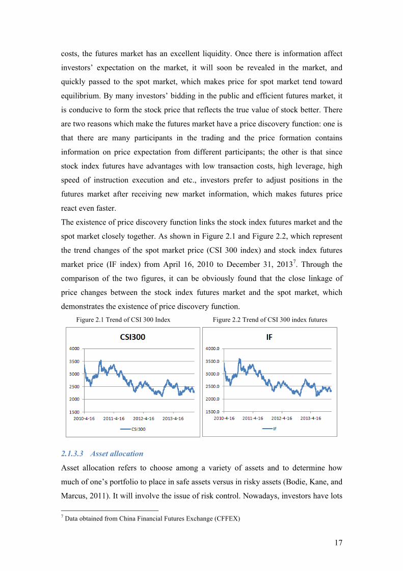
The existence of price discovery function links the stock index futures market and the

spot market closely together. As shown in Figure 2.1 and Figure 2.2, which represent

the trend changes of the spot market price (CSI 300 index) and stock index futures

market price (IF index) from April 16, 2010 to December 31, 20137. Through the

comparison of the two figures, it can be obviously found that the close linkage of

price changes between the stock index futures market and the spot market, which

demonstrates the existence of price discovery function. Figure 2.1 Trend of CSI 300 Index Figure 2.2 Trend of CSI 300 index futures

2.1.3.3 Asset allocation

Asset allocation refers to choose among a variety of assets and to determine how

much of one’s portfolio to place in safe assets versus in risky assets (Bodie, Kane, and

Marcus, 2011). It will involve the issue of risk control. Nowadays, investors have lots

7 Data obtained from China Financial Futures Exchange (CFFEX)

18

of investment choices, such as stocks, bonds, real estate, commodities and so on.

However, most of the investment cannot get rid of systemic risk. The most obvious

example is the subprime crisis after 2007. When the whole environment was bad,

almost all the investment facing losses; but in futures market, many investors who are

in the short positions have made bundles of money; such as George Soros, based on

his experience during this period, he has published a book called “The new paradigm

for financial markets: the credit crisis of 2008 and what it means”.

The transaction costs involved in establishing and liquidating futures positions are

much lower than taking actual spot positions, so that many institutional investors

consider the stock index futures as a flexible asset allocation tool (Bodie, Kane, and

Marcus, 2011).

Asset allocation function shows specifically in the following areas: First, due to the

introduction of short-mechanism, the investment strategy of investors changes from

the single mode (waiting stock price rise) into the mode (a two-way investment),

which makes the investors’ funds can also be something even in the downward

market trend, rather than passively unused; Second, the stock index is a stock

portfolio itself; it conforms with the basic principle of investment diversification, and

reduces significantly the risk compared to the specific stock trading, which is

particularly conducive to the development of institutional investors, portfolio

investment promotion and risk management; Third, through the trading of stock index

futures, it can adjust the proportion of various types of assets in the portfolio, increase

the market liquidity and improve the efficiency of capital using. When investors want

to increase or decrease the amount of the financial asset holdings, they can just buy or

sell stock index futures contracts corresponding to the asset.

2.2 Related theory of hedging

2.2.1 Concept

Hedging is undertaken to reduce the price risk of a cash or forward position by taking

a position in the futures instrument to offset the price movement of the cash asset

(Daigler, 1993). In a broader sense, it uses futures as a temporary substitute for the

cash position. So, hedging can be regarded as a management tool. When it is suitable

for an organization, it helps to reduce risk and improve working capital potions. Its

effectiveness can be evaluated quantitatively. Its ability to reduce price level risk

serves as economic justification. Hedging should always be viewed as risk reducing

19

but not eliminating, thus it is required that the remaining risk should be identified and

monitored (Chance & Brooks, 2008).

2.2.2 Economic principles

Generally speaking, a hedge is simply the purchase (sale) of a futures market position

as a temporary substitute for the security of the sale (purchase) in the cash market.

Hedgers in the futures market will always take an opposite position to the cash

position held. In a hedge, risk is reduced to the extent that the gain (loss) in the future

position offsets the loss (gain) on the cash position. To achieve the function of

hedging, it is based on the following economic principles:

• The price in the cash market and the price in the futures market will generally

change in the same direction. Although the spot market and futures market are

two completely separate markets, the economic factors and the economic

environment that affect the spot price and the futures price are similar.

Therefore, theoretically speaking, the price-changing tendency in both markets

is the same. Hedgers can achieve the purpose of hedging based on this

principle.

• As the futures contract nears delivery, the spot and futures prices will

converge; as expiration approaches, the futures price equals or is very close to

the spot price. Because of above principle, futures prices should equal to the

spot prices on the maturity date. Once the prices are not equal, there will be

risk-free arbitrage trading opportunities existing for traders. Then, the

arbitrageurs8 will quickly take advantage of this spread that would equalize the

prices. The arbitrageurs can restrict the fluctuation of price.

• Hedging transfers the spot prices as the basis risk in futures market, which can

reduce the risk in spot market. Typically, hedging is the shifting of risk from

hedgers to speculators or to the marketplace. Hedging reduces the gain

potential as well as the loss potential (Chance&Brooks, 2008). More

specifically, it is the process, which transforms the potentially more hazardous

price level risk into the more manageable basis risk.

8 These apparent mispricing lead to the presence of “arbitrageurs,” who aim to exploit the resulting profit opportunities, but whose role remains controversial.

20

2.2.3 Types

There are two types of hedges, i.e. the short hedge and the long hedge; also known as

sell and buy hedges.

A short hedge is a hedge that involves a short position in futures contracts in order to

offset adverse price changes in a long cash position (Hull, 2012). When the investors

forecast a decline in the price of stocks, the investors can execute a short hedge with a

future contract to “lock-in” the price of stock portfolio that will be purchased in the

future. So, by selling stock futures short, the investors on the futures side, could

partially or totally offset the loss on the long cash stock position as its price declines.

Typically, organizations that maintain inventories (such as securities trading firms,

refiners, or commodity producers) tend to be short hedgers. They sell futures or enter

sale agreements to protect inventory or portfolio values.

As for long hedging, it is usually considered to be taking futures positions as

substitute for a short cash position (Blank, Carter and Schmiesing, 1991). A long

hedge is initiated when futures contracts are purchased in order to “lock-in” a price

now and prevent the risk of price variability. Long hedges can be used to manage an

existing short position. For example, if a hedger knows he will buy some amount of

stock in the future, he can buy stock index futures immediately in the futures market.

Thus, he can lock in the current value and only pay a small amount for the margin

deposit.

According to the different purpose of hedging, it can be divided as the positive

hedging and the passive hedging (Gregoriou, 2011).

• Positive hedging

The objective of positive hedging is to maximize revenues. Through the predictions

on the stock market trends, it can choose hedging strategy wisely to avoid systemic

risk. When the portfolio manager is facing greater systemic risk, he can use the

positive hedging to hedge the systemic risk of the portfolio. However, this is just a

temporary choice, after the release of risk, it will close the position.

• Passive hedging

The passive hedging sets its goal as the risk-averse, regardless of the revenue

increment due to its operation. It does not involve stock market forecast. The purpose

is to reduce or even completely avoid the systemic risk in the spot market. For this

21

purpose, what matters is not the profit made through the stock index futures, but the

certainty of stock price in the spot market by holding stock index futures.

2.2.4 The Basis Theory

The basis defines the quantitative relationship that exists between the physical

position and the hedge instrument (Koziol, 1990). Basis is the difference between the

spot price and the futures price of the same commodity or asset (Schwarz, Hill and

Schneeweis, 1986). The basis is decreasing over time as expiration nears. The

convergence of prices eventually drives the gross basis9 to zero (Cusatis & Thomas,

2005). Basis is an important index that the hedger should concern. The changing

trends of basis affect the hedge effectiveness of stock index futures directly. Its

change provides important criteria for the investors, which can have the rational asset

allocation and choose the right hedging strategy. The basis in a hedging situation can

be expressed as follows: Basis = Spot price of asset to be hedged – Futures price of contract used

There will be a different basis for each delivery month for each contract. Moreover,

this relationship should be acceptably stable. This does not mean that the basis cannot

fluctuate but rather it should not do so in an erratically volatile manner.

2.2.4.1 Basis risk

In general, hedging should follow the four basic principles:

• Opposite trading direction

It requires holding the opposite positions in the spot and futures markets. It is

the most important one. Only following this rule, investors can gain in one

market, and offset the loss in another market.

• Same or relevant variety of trade

When creating a hedging portfolio, the futures should be consistent with the

chosen spot goods. In this way, it can create a close relationship between the

futures price and the spot price. They will have the same price trend.

• Same transaction amount

It requires the futures contracts have the same value of underlying assets in the

spot market; otherwise, there will face greater risk.

• Same or similar month

9 Gross basis is measured as the difference between the two prices at the close of each business day.

22

It would be better that the delivery month of futures contract is the same with

the time of buying or selling assets in the spot market. It can improve the

effect of hedging.

However, in the real situation, the perfect hedging hardly ever happens, since any

change of factors that affects the spot price or the futures price will induce the change

of basis. Basis change leads to the uncertainty of hedging effectiveness, which is

called basis risk.

2.2.4.2 Affecting factors of basis risk

For stock index futures, the affecting factors of basis risk are mainly reflected in the

following aspects (Dubofsky & Miller, 2003):

• Change of supply and demand in constituent stocks

When the demand of constituent stocks is greater than the supply, the spot

price would be lower than the futures price. It will drive the basis change to

the opposite direction.

• Changes in interest rates

Assume the stock yield of a company has not changed, if the interest rate rises,

the price of stock index futures will be greater than the spot price. The basis

will increase in reverse direction. If the market interest rate decline, the spot

price will be more than the futures price, the basis is said to strengthen.

• Changes in stock yield10

If the company's stock yield rises, then the basis is said to strengthen.

Conversely, when the stock yields drop, the basis is said to weaken.

• Policy factors

If monetary policy or fiscal policy changes in the economic development, then

the exchange rate, interest rate, inflation rates and other economic indicators

will be affected. Consequently, the futures price and the spot price are going to

be influenced.

In hedging, the trader still faces basis risk. However, the change range of basis is

smaller than the price change in the futures market or the spot market. Traders can

reduce their investment risks by using basis risk to replace price risk in the futures

market or the spot market. Rational traders tend to choose this way to hedge.

10 Stock yield is the dividend per share divided by its current price per share

23

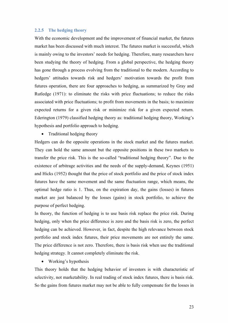
2.2.5 The hedging theory

With the economic development and the improvement of financial market, the futures

market has been discussed with much interest. The futures market is successful, which

is mainly owing to the investors’ needs for hedging. Therefore, many researchers have

been studying the theory of hedging. From a global perspective, the hedging theory

has gone through a process evolving from the traditional to the modern. According to

hedgers’ attitudes towards risk and hedgers’ motivation towards the profit from

futures operation, there are four approaches to hedging, as summarized by Gray and

Rutledge (1971): to eliminate the risks with price fluctuations; to reduce the risks

associated with price fluctuations; to profit from movements in the basis; to maximize

expected returns for a given risk or minimize risk for a given expected return.

Ederington (1979) classified hedging theory as: traditional hedging theory, Working’s

hypothesis and portfolio approach to hedging.

• Traditional hedging theory

Hedgers can do the opposite operations in the stock market and the futures market.

They can hold the same amount but the opposite positions in these two markets to

transfer the price risk. This is the so-called “traditional hedging theory”. Due to the

existence of arbitrage activities and the needs of the supply-demand, Keynes (1951)

and Hicks (1952) thought that the price of stock portfolio and the price of stock index

futures have the same movement and the same fluctuation range, which means, the

optimal hedge ratio is 1. Thus, on the expiration day, the gains (losses) in futures

market are just balanced by the losses (gains) in stock portfolio, to achieve the

purpose of perfect hedging.

In theory, the function of hedging is to use basis risk replace the price risk. During

hedging, only when the price difference is zero and the basis risk is zero, the perfect

hedging can be achieved. However, in fact, despite the high relevance between stock

portfolio and stock index futures, their price movements are not entirely the same.

The price difference is not zero. Therefore, there is basis risk when use the traditional

hedging strategy. It cannot completely eliminate the risk.

• Working’s hypothesis

This theory holds that the hedging behavior of investors is with characteristic of

selectivity, not marketability. In real trading of stock index futures, there is basis risk.

So the gains from futures market may not be able to fully compensate for the losses in

24

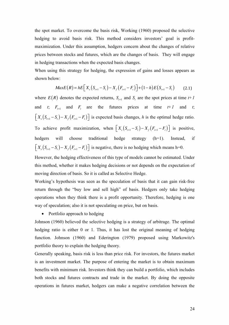
the spot market. To overcome the basis risk, Working (1960) proposed the selective

hedging to avoid basis risk. This method considers investors’ goal is profit-

maximization. Under this assumption, hedgers concern about the changes of relative

prices between stocks and futures, which are the changes of basis. They will engage

in hedging transactions when the expected basis changes.

When using this strategy for hedging, the expression of gains and losses appears as

shown below:

MaxE R( ) = hE Xs St+1 − St( )− X f Ft+1 − Ft( )⎡⎣ ⎤⎦ + 1− h( )E St+1 − St( ) (2.1)

where E R( ) denotes the expected returns, St+1 and St are the spot prices at time t+1

and t; Ft+1 and Ft are the futures prices at time t+1 and t;

Xs St+1 − St( )− X f Ft+1 − Ft( )⎡⎣ ⎤⎦ is expected basis changes, h is the optimal hedge ratio.

To achieve profit maximization, when Xs St+1 − St( )− X f Ft+1 − Ft( )⎡⎣ ⎤⎦ is positive,

hedgers will choose traditional hedge strategy (h=1). Instead, if

Xs St+1 − St( )− X f Ft+1 − Ft( )⎡⎣ ⎤⎦ is negative, there is no hedging which means h=0.

However, the hedging effectiveness of this type of models cannot be estimated. Under

this method, whether it makes hedging decisions or not depends on the expectation of

moving direction of basis. So it is called as Selective Hedge.

Working’s hypothesis was seen as the speculation of basis that it can gain risk-free

return through the “buy low and sell high” of basis. Hedgers only take hedging

operations when they think there is a profit opportunity. Therefore, hedging is one

way of speculation; also it is not speculating on price, but on basis.

• Portfolio approach to hedging

Johnson (1960) believed the selective hedging is a strategy of arbitrage. The optimal

hedging ratio is either 0 or 1. Thus, it has lost the original meaning of hedging

function. Johnson (1960) and Ederington (1979) proposed using Markowitz's

portfolio theory to explain the hedging theory.

Generally speaking, basis risk is less than price risk. For investors, the futures market

is an investment market. The purpose of entering the market is to obtain maximum

benefits with minimum risk. Investors think they can build a portfolio, which includes

both stocks and futures contracts and trade in the market. By doing the opposite

operations in futures market, hedgers can make a negative correlation between the

25

assets in spot market and the assets in futures market. So that the portfolio can obtain

a satisfy combination of return and risk.

Therefore, in addition to do hedging selectively, the amount of buying and selling

futures contracts is not necessarily consistent with the amount of spot transactions.

Hedgers can adjust and change the amount of futures trading anytime, according to

their purpose and the relationship between futures price and stock prices any time to

select an optimal hedge ratio.

Portfolio theory is an important part of the modern hedging theory. By combining

stocks and futures as a portfolio, it stresses that the optimal hedging ratio is not 0 or 1.

Moreover, it avoids risks rationally through simulation to estimate the effective

hedging ratio. And it fully considers the profits and risks of the existence of portfolio

to illustrate the relevant hedging purposes.

26

3 Development of stock index futures in China It can be seen from former chapters, the stock index futures is already one of the basic

derivative financial instruments in mature markets, and the foreign investors have a

deep understanding on it. However, it is the first time that China release stock futures

contracts. The investors in China may not have relatively sufficient knowledge, and

normally the kinds of stock index futures products are not the same in different

countries. Moreover, different products have their own characteristics in different

market environments. To deeply understand the characteristics of stock index futures

in a specific environment, we must fully understand the relevant knowledge of the

subject matter and its trading mechanism. In this chapter, the development of stock

market and stock index futures in China and its related knowledge about CSI 300 will

be focused.

3.1 Development of stock market in China Due to the complexity of the Chinese economy and the imperfection of China’s

capital markets, the implementation of stock index futures in China has undergone

many ups and downs.

3.1.1 Chinese stock market

Chinese Stock Market has undergone a substantial development since its

establishment in the early 1990’s. The large increases in share prices and market

capitalization mainly benefit from the liberalization of market and the improvement of

investor protection. The Chinese stock market is a typically immature and emerging

capital market. There are many disparities between the Chinese stock market and

mature capital markets of developed countries and regions, such as their backgrounds

of establishment, modes of operation and developing processes. The regulatory roles

and the national macroeconomic policies on these two types of markets are also very

different, e.g. the development of the Chinese capital markets has been mainly driven

by the central government.

When talking about China’s stock market, it has to include both the stock markets in

the Mainland China as well as in the Hong Kong Special Administrative Region,

because the HK market has become an integral part of the overall China market11. The

organized stock market in Mainland China is composed of two stock exchanges, the

11 China Stock Market Handbook

27

Shanghai stock exchange (SSE) and the Shenzhen stock exchange (SZSE). Since

1992, the Chinese stock market has boomed and become one of the worldwide largest

in a relatively short lapse of time. The stock market in China averaged 1680.01 index

points from 1990 until 2014, reaching an all time high of 6092.06 index points in

October of 200712. Starting from 53 in 1992, the number of firms listed on SSE and

SZSE increased 50 times to 2,532 in 2013 (see Figure 3.1). After the rally in 2007, the

Chinese stock market reached a market capitalization of over 30 trillion Yuan. This

volume overstepped China’s nominal GDP for the first time13. Figure 3.1 Number of listed firms, 1992-2013

Source: CSRC.

3.1.2 Reform of Chinese stock market

In recent years, with the continuous reform of the financial markets in depth, the

marketization of interest rates in China makes the demands of risk management tools

increase rapidly, especially for the financial institutions. Also, non-tradable shares

reform, which is a special appearance during the development of corporate system

and capital market, has been implemented in the Mainland of China. And Chinese

government resolutely carries out reform of the shareholder structure in listed

companies and resolves this longstanding institutional problem that hindered the

development of the securities market, which hopefully build a good environment for

the development of stock index futures.

Basically, China's shares are divided into state shares, legal person shares, individual

shares and foreign shares. And the state shares and legal person shares cannot

12 Data obtained from Shanghai Shenzhen Stock Exchange. 13 Data obtained from CSRC annual report, http://www.csrc.gov.cn/pub/newsite/xxfw/cbwxz/tjnj/zqqhtjnj/2012/main/index2.htm

0  500  1000  1500  2000  2500  3000  

No.  

Year  

Number  of  listed  <irms  

28

circulate, but individual shares and foreign shares can be traded on the Shanghai and

Shenzhen Stock Exchange. Most legal persons are actually state entities, so the legal

person shares and state shares are known as state-owned shares (Luo, 2011).

The stock market enables companies to become openly exchanged, or even increase

extra funds with regard to growth selling off stocks. However, the non-tradability of

state-owned shares led to many problems, which limited the development of stock

market. Firstly, state assets were “dead”, which would be less valuable; secondly,

property rights of enterprises could not be clearly defined among individual investors;

thirdly, capital mobility and economic restructuring were hindered; and lastly, the

development of a secondary stock market was obstructed (Ma, 2008). Thus, it could

be expected that if the proportion of state ownership in Chinese enterprises could

decrease further, the development of stock market would be better. However, from

1997-2004, there were only minor changes in the relative size of the state–owned

shares (Ma, 2008).

A breakthrough occurred in late April 2005. Under the guidance of the State Council,

the China Securities Regulatory Commission (CSRC) launched the Equity Division

Reform among Chinese listed companies. The CSRC explained that the reform was

designed to address the problem of non-tradability of the large amount of state-owned

shares, instead of cashing them in. It is a historical residual problem from the period

before the companies went public. The coexistence of non-tradable state-owned

shares and tradable individual shares has resulted in a “dualistic” market consisting of

“different types of equities, different prices, and different rights” (Ma, 2008). In late

2006, Shang Fulin, chairman of the CSRC, announced that the reform “had basically

been accomplished.”14 In 2008, there were a total of 1656 listed companies have

finished the reform or in the reform process in Shanghai stock market and Shenzhen

stock market. It has reached 98.6% of the listed companies who should have

implemented the reform15.

Technically, the reform was to correct the system error, and to resume original

feature, to make non-circulating stocks to become circulating stocks, to realize the

same stock has same price, right and profit. The reform sought to remove the

problems regarding the split share structure and the negative effects of dividends on

14 Shanghai Zhengquan Bao, January 15, 2007. 15 Data obtained from the news of Financial Times (in Chinese) http://www.ftchinese.com/story/001043496

29

the A-share investors.

During the reform period from 2005 to 2008, the smooth progress of the split share

structure reform fundamentally solved the problem of dividing interests and prices

among the state-owned shares, institutional shares and tradable shares in a company’s

share structure. And it enabled equal rights to the trading of and earnings on shares

among all categories of shareholders (OECD).

It can be seen that promoting the non-tradable share reform has a great practical

significance to build up market confidence and bring steady growth of investment.

Also owing to this reform, the market foundation is strengthened. China’s shares are

now valued by the market mechanism that creates the basis for common interests of

all shareholders. On the other hand, the quality of listed companies is also getting

promoted. The internal control mechanism of brokers and futures companies has

being gradually perfected. All these advantages have created a favorable environment

for the introduction of stock index futures.

3.2 Development of CSI 300 index futures In order to better reflect the price fluctuation and general performance of China A-

share market, China Securities Index 300 (CSI 300), designed and managed by China

Securities Index Co., Ltd, was launched on April 8, 2005. The mock trading16 of CSI

300 index futures was put into operation by the China Financial Futures Exchange

(CFFEX) on 30th October 2006. Till April 2007, the Regulation on the Administration

of Futures Trading was issued by the State Council17, which cleared the way for the

trading of stock index futures. By the end of 2006, it was more than doubled in less

than two years. The exchange and market participants expected the CSRC agreed to

implement the real trading of stock index futures from 2007. But the stock market was

on a tear. The CSRC was afraid of the introduction of stock index futures might cause

the stock market bubble. So the approval was withheld by CSRC. Since the outbreak

of the global financial crisis in 2008, the regulators feared that the futures might

aggravate the bear market. The year 2008 was a bad year for all capitalist markets

especially the SSE. Its benchmark recorded its biggest annual loss of more than 65%.

It fell from 5265 points in January 2008 to 1834 points in December 200818. Hence,

16 The difference between mock trading and real trading is that the money is not real. 17 http://www.lawinfochina.com/display.aspx?lib=law&id=5948&CGid= 18 Data obtained from Yahoo Finance, http://finance.yahoo.com/q?s=000001.SS

30

the mock trading was not changed to a real one but continued by CFFEX in year 2008,

2009 and into 2010.

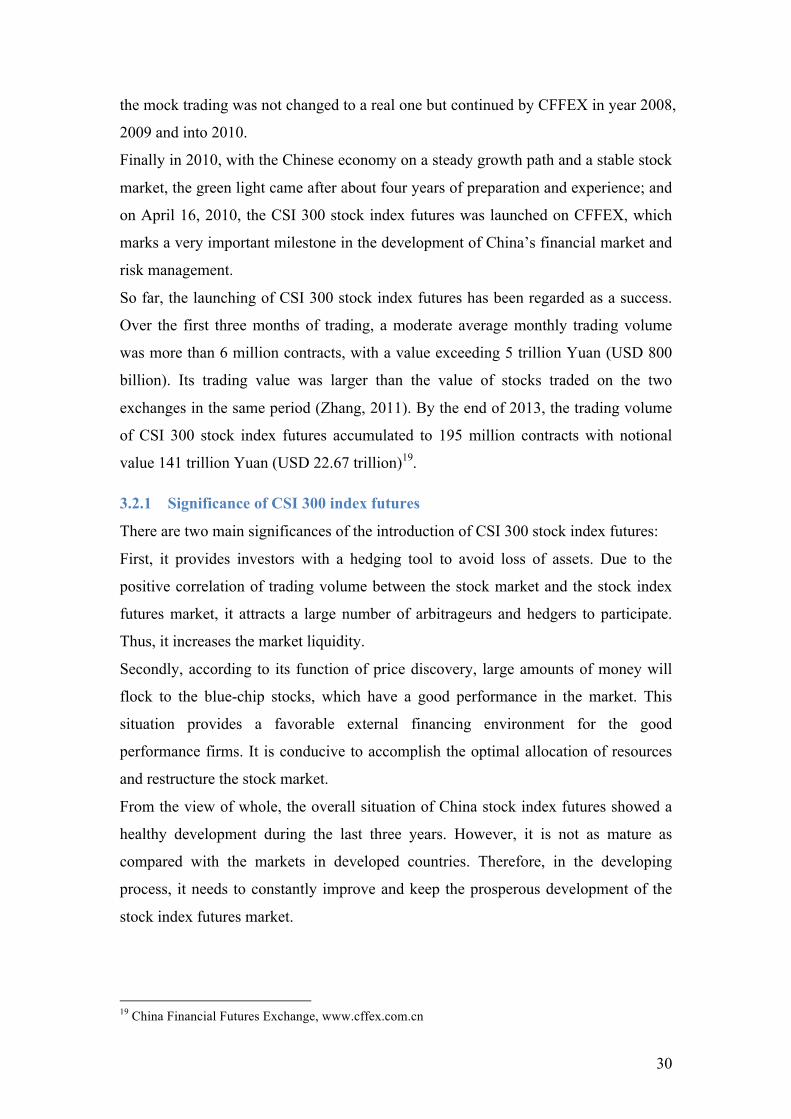
Finally in 2010, with the Chinese economy on a steady growth path and a stable stock

market, the green light came after about four years of preparation and experience; and

on April 16, 2010, the CSI 300 stock index futures was launched on CFFEX, which

marks a very important milestone in the development of China’s financial market and

risk management.

So far, the launching of CSI 300 stock index futures has been regarded as a success.

Over the first three months of trading, a moderate average monthly trading volume

was more than 6 million contracts, with a value exceeding 5 trillion Yuan (USD 800

billion). Its trading value was larger than the value of stocks traded on the two

exchanges in the same period (Zhang, 2011). By the end of 2013, the trading volume

of CSI 300 stock index futures accumulated to 195 million contracts with notional

value 141 trillion Yuan (USD 22.67 trillion)19.

3.2.1 Significance of CSI 300 index futures

There are two main significances of the introduction of CSI 300 stock index futures:

First, it provides investors with a hedging tool to avoid loss of assets. Due to the

positive correlation of trading volume between the stock market and the stock index

futures market, it attracts a large number of arbitrageurs and hedgers to participate.

Thus, it increases the market liquidity.

Secondly, according to its function of price discovery, large amounts of money will

flock to the blue-chip stocks, which have a good performance in the market. This

situation provides a favorable external financing environment for the good

performance firms. It is conducive to accomplish the optimal allocation of resources

and restructure the stock market.

From the view of whole, the overall situation of China stock index futures showed a

healthy development during the last three years. However, it is not as mature as

compared with the markets in developed countries. Therefore, in the developing

process, it needs to constantly improve and keep the prosperous development of the

stock index futures market.

19 China Financial Futures Exchange, www.cffex.com.cn

31

3.3 CSI 300 Index and CSI 300 stock index futures

3.3.1 Pricing CSI 300 Index

China Securities Index (CSI) 300 is an index that consists of 300 stocks with the

largest market capitalization and liquidity from all the A-share listed companies. As

the first equity index launched by the two exchanges together, CSI 300 Index was

created with the base point at 1000 on December 31, 2004. The candidate constituents

of CSI 300 index should have good performance without serious financial problems

(or laws and regulations breaking events) and with no large price volatility, which can

represent strong evidence of manipulated20.

CSI 300 index is calculated using a Paasche21 weighted composite price index

formula and is weighted by adjusted shares22. For pricing CSI 300 index, no

adjustment is required for dividend payment and the index is allowed to fallback

naturally. But for total return index and net total return index, the divisor will be

adjusted before the ex-dividend date.23

3.3.2 Relation with Shanghai index and Shenzhen index

The most important indices for A-shares24 in SSE and SZSE are the Shanghai stock

exchange composite index and the Shenzhen stock exchange component index.

The Shanghai SE Composite Index is a major stock market index which tracks the

performance of all A-shares and B-shares listed on the Shanghai Stock Exchange, in

China. It is a capitalization-weighted index. And the Shenzhen Stock Exchange

Component Index is a Capitalization Weighted Index. The constituents consist of the

40 top companies that issue A-shares on Shenzhen Stock Exchange.25

The correlation between the CSI 300 index and the Shanghai Composite Index has

been 97% at the beginning. Though the CSI 300 index do not have a clearly relevance

with the Shenzhen Index; by the end of 2013, the total market capitalization of CSI

300 Index is 14.14 trillion Yuan and its free float market capitalization is 5.19 billion

20 CSI 300 Handbook, http://www.csindex.com.cn/sseportal_en/csiportal/xzzx/file/CSI300%20Handbook.pdf 21 Paasche index uses quantities for each period as weights and compares current prices to base period prices at current purchase levels. 22 Formula and table can be found in Appendix A. 23 CSI 300 Methodology, http://www.csindex.com.cn/sseportal_en/csiportal/xzzx/file/CSI300methodology.pdf 24 RMB-denominated ordinary shares for domestic residents and institutions to invest in are called A-shares for short. 25 Both of the two indexes are not required for index adjustment when dividend payment happened.

32

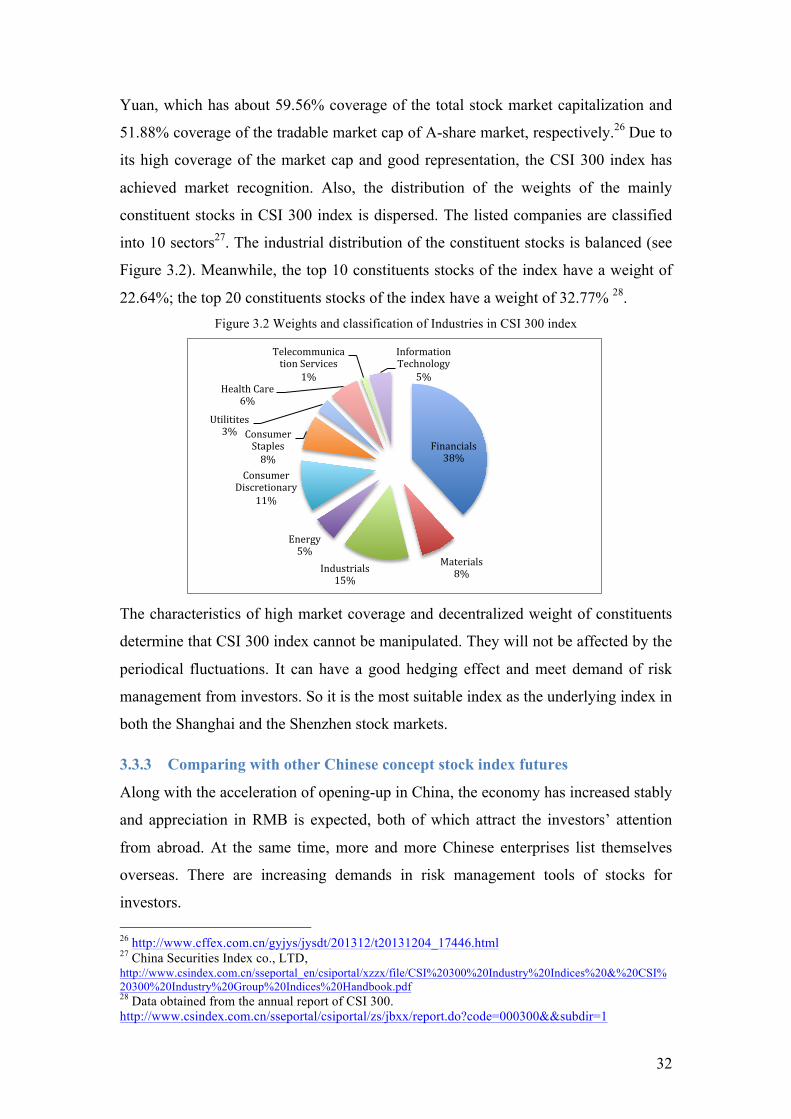
Yuan, which has about 59.56% coverage of the total stock market capitalization and

51.88% coverage of the tradable market cap of A-share market, respectively.26 Due to

its high coverage of the market cap and good representation, the CSI 300 index has

achieved market recognition. Also, the distribution of the weights of the mainly

constituent stocks in CSI 300 index is dispersed. The listed companies are classified

into 10 sectors27. The industrial distribution of the constituent stocks is balanced (see

Figure 3.2). Meanwhile, the top 10 constituents stocks of the index have a weight of

22.64%; the top 20 constituents stocks of the index have a weight of 32.77% 28. Figure 3.2 Weights and classification of Industries in CSI 300 index

The characteristics of high market coverage and decentralized weight of constituents

determine that CSI 300 index cannot be manipulated. They will not be affected by the

periodical fluctuations. It can have a good hedging effect and meet demand of risk

management from investors. So it is the most suitable index as the underlying index in

both the Shanghai and the Shenzhen stock markets.

3.3.3 Comparing with other Chinese concept stock index futures

Along with the acceleration of opening-up in China, the economy has increased stably

and appreciation in RMB is expected, both of which attract the investors’ attention

from abroad. At the same time, more and more Chinese enterprises list themselves

overseas. There are increasing demands in risk management tools of stocks for

investors. 26 http://www.cffex.com.cn/gyjys/jysdt/201312/t20131204_17446.html 27 China Securities Index co., LTD, http://www.csindex.com.cn/sseportal_en/csiportal/xzzx/file/CSI%20300%20Industry%20Indices%20&%20CSI%20300%20Industry%20Group%20Indices%20Handbook.pdf 28 Data obtained from the annual report of CSI 300. http://www.csindex.com.cn/sseportal/csiportal/zs/jbxx/report.do?code=000300&&subdir=1

Financials  38%  

Materials  8%  Industrials  

15%  

Energy  5%  

Consumer  Discretionary  

11%  

Consumer  Staples  8%  

Utilitites  3%  

Health  Care  6%  

Telecommunication  Services  

1%  

Information  Technology  

5%  

33

Under this background, the Hong Kong stock exchange (HKEx), Singapore stock

exchange (SGX) and Chicago Mercantile exchange (CME) have launched a series of

stock index futures with Chinese Concept before the CSI 300 index futures. They

have attracted a large number of investors to participate in. Since the day of

introducing CSI 300 index futures, it is facing the competition with the overseas

Chinese concept stock index futures. Generally speaking, the more relatively

homogeneous products and the better the alternative emerge, the stronger competition

is between each other.

• H-shares index futures29

Hong Kong Exchange launched H-shares index futures on Dec. 8 2003. It is a first

overseas Chinese concept stock index future. Its underlying index is Hang Seng China

Enterprise Index (HSCEI). It is a market capitalization-weighted stock index. It tracks

the performance of Mainland China enterprises with H-share listings in Hong Kong.

The 40 stocks that have the highest combined market capitalization ranking are

selected as constituents of the H-shares Index. Compared with CSI 300, through the

analysis of the constituents of the HSCEI, there is an overlap of most heavyweights

stocks in the two indexes (see Appendix B). This indicated that CSI 300 and HSCEI

are highly correlative.

• Mini H-shares index futures30

Mini H-shares index futures would meet the needs of customers who have a smaller

risk capital31. The underlying index is HSCEI, as well as the standard H-shares Index

futures contract. The smaller contract size allows both experienced and novice

investors to participate in the performance of the H-shares market in a graduated

scale.

• E-mini FTSE/Xinhua China 25 Index futures

CME listed E-mini(R) futures on the FTSE/Xinhua(R) China 25 Index. The FXI

China 25 index is composed by 25 of the largest Chinese companies listed on the

Hong Kong Stock Exchange and has a total market capitalization of about USD 241

billion.32 Due to the constituents of the index including red chips, which have not

returned to A-share market, the correlation between FXI China 25 index and CSI 300

index is weaker. 29 https://www.hkex.com.hk/eng/prod/drprod/hshares/hshares_product.htm 30 https://www.hkex.com.hk/eng/prod/drprod/mchfut/mchprodes.htm 31 Risk capital refers to funds used for high-risk, high-reward investments. 32 http://investor.cmegroup.com/investor-relations/releasedetail.cfm?ReleaseID=233777

34

• SGX FTSE China A50 Futures

Denominated in U.S. dollar, the SGX A50 Futures are the only offshore futures

tracking the China A-shares market. It is based on the FTSE China A50 Index, which

tracks the performance of the largest 50 companies by full market capitalization on

the Chinese stock market. 33 The index offers the optimal balance between

representativeness and tradability for China’s A Share market. The constituents of

CSI 300 index covered the all constituents of FTSE China A50 index. Table 3.1 Comparison among the index futures

Exchanges Name of stock index futures Substitutability Competitiveness

HKEX (Hong Kong

Stock Exchange)

H-shares index futures Strong Strong

Mini H-shares index futures

E-mini FTSE/Xinhua China

25 Index futures

Weak Weak

SGX (Singapore

Exchange)

SGX FTSE China A50

Futures34

Strong Weak

CME (Chicago

Mercantile Exchange)

E-mini FTSE/Xinhua China

25 Index futures

Weak Weak

Note. Substitutability here stands for if CSI 300 index futures can be replaced by other futures.

Based on the above analysis, the H-shares index futures is a strong competitor of CSI

300 index futures. Due to the index design and its requirement from the stock market,

CSI 300 index has its own competitive advantage. The trading volume and trading

value related to the constituent stock of CSI 300 index futures are far more than them

related to the constituent stock of H-share index futures (Fang, 2008). Apparently, it is

clear that investing in the Mainland China stock market makes a number of fund

companies, insurance companies, QFII35 and other institutional investors have a great

demand to hedge the stock risk. In addition, as mentioned before, CSI 300 Index

could be a good representative in terms of market scale, liquidity, and industry group

of A-share market.

For the introduction of CSI 300 Index, it is not only able to reflect the operating

conditions and the trend of price volatility of China’s A-share market

comprehensively and truly, but it also provides some reference value to the stock

investment of the investors. Meanwhile, it establishes the foundation for the launching

33 http://news.xinhuanet.com/english/china/2013-10/11/c_132790137.htm 34 SGX A 50 futures has law issues with the two stock exchanges in China. 35 QFII: Qualified Foreign Institutional Investor.

35

of CSI 300 stock index futures.

3.3.4 Comparing CSI 300 index futures contract with H-shares index futures

contract

Some features of CSI 300 index futures contract36 and H-shares index futures

contract37 can be seen in Table 3.2. Table 3.2 Comparison between two contracts

Contract CSI 300 index futures H-shares index futures

Underlying Index CSI 300 Index Hang Seng China Enterprises Index

(HSCEI)

Contract

Multiplier

CNY 300 HK$ 50

Unit Index point Index point

Tick Size38 0.2 point One index point

Contract Months Current month, next month,

next two calendar quarters

Spot month, next calendar month,

next two calendar quarter months

Pre-Market

Opening Period

None 8:45 am - 9:15 am & 12:30 pm - 1:00

pm

Trading Hours 09:15 am - 11:30 am, 1:00 pm -

3:15 pm

9:15 am - 12:00 noon, 1:00 pm - 4:15

pm & 5:00 pm - 11:00 pm39

Trading Hours on

Last Trading Day

09:15 am - 11:30 am, 1:00 pm -

3:00 pm

Expiring contract month closes at

4:00 pm on the Last Trading Day

Limit Up/Down +/-10% of settlement price on

the previous trading day

Margin

Requirement

12% of the contract value Initial HK$ 31,400 per

lot

Maintenance HK$ 25,150 per

lot

Last Trading Day Third Friday of the contract

month, postponed to the next

business day if it falls on a

public holiday

The Business Day immediately

preceding the last Business Day of

the Contract Month

36 http://www.cffex.com.cn/en_new/sspz/hs300zs/ 37 https://www.hkex.com.hk/eng/prod/drprod/hshares/hhifut.htm 38 Tick size means Minimum fluctuation 39 Hong Kong Exchanges and Clearing Limited (HKEx) has introduced After-Hours Futures Trading (AHFT) since 8 April 2013, which means the trading is still open from 5 pm to 11 pm. But AHFT is not applicable on last trading day and the pre market opening period.

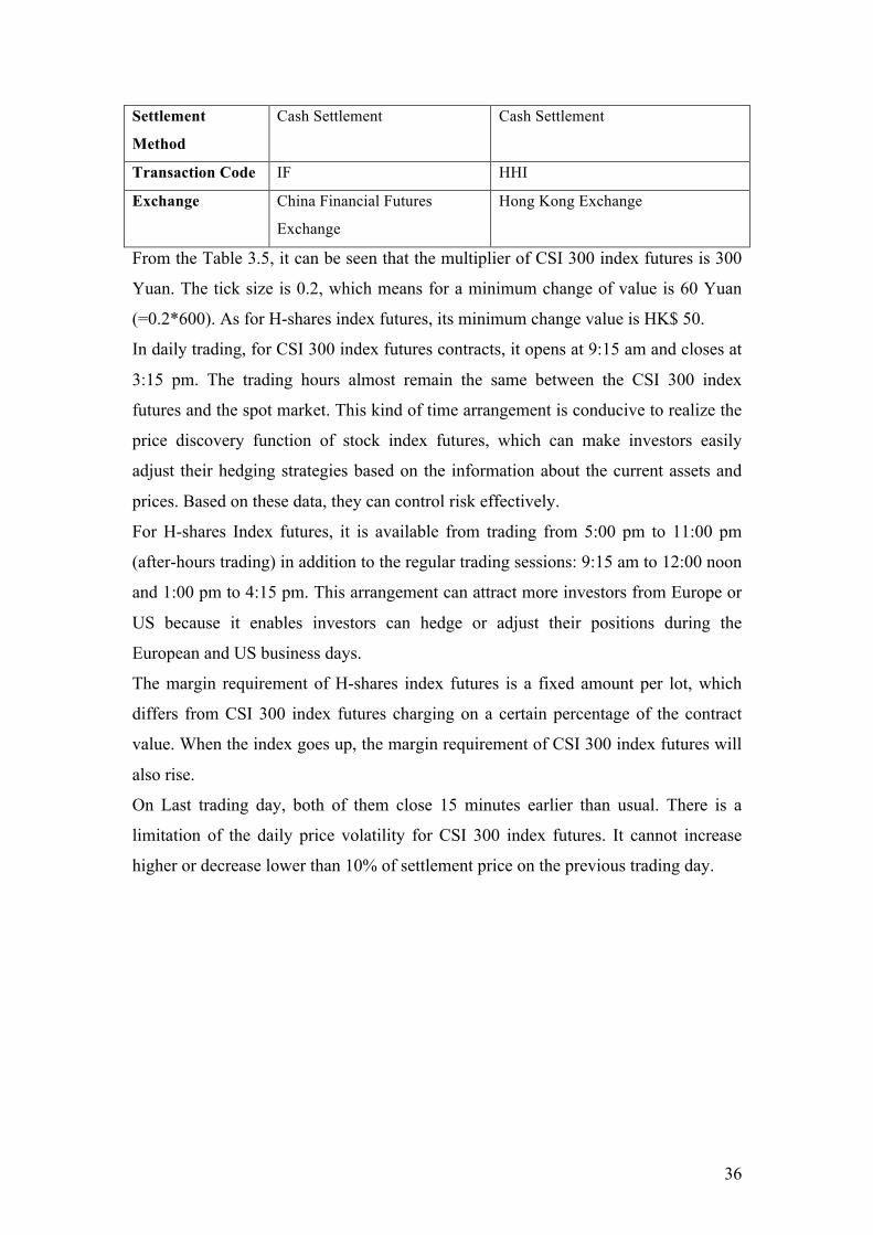
36

Settlement

Method

Cash Settlement Cash Settlement

Transaction Code IF HHI

Exchange China Financial Futures

Exchange

Hong Kong Exchange

From the Table 3.5, it can be seen that the multiplier of CSI 300 index futures is 300

Yuan. The tick size is 0.2, which means for a minimum change of value is 60 Yuan

(=0.2*600). As for H-shares index futures, its minimum change value is HK$ 50.

In daily trading, for CSI 300 index futures contracts, it opens at 9:15 am and closes at

3:15 pm. The trading hours almost remain the same between the CSI 300 index

futures and the spot market. This kind of time arrangement is conducive to realize the

price discovery function of stock index futures, which can make investors easily

adjust their hedging strategies based on the information about the current assets and

prices. Based on these data, they can control risk effectively.

For H-shares Index futures, it is available from trading from 5:00 pm to 11:00 pm

(after-hours trading) in addition to the regular trading sessions: 9:15 am to 12:00 noon

and 1:00 pm to 4:15 pm. This arrangement can attract more investors from Europe or

US because it enables investors can hedge or adjust their positions during the

European and US business days.

The margin requirement of H-shares index futures is a fixed amount per lot, which

differs from CSI 300 index futures charging on a certain percentage of the contract

value. When the index goes up, the margin requirement of CSI 300 index futures will

also rise.

On Last trading day, both of them close 15 minutes earlier than usual. There is a

limitation of the daily price volatility for CSI 300 index futures. It cannot increase

higher or decrease lower than 10% of settlement price on the previous trading day.

37

4 The general principle of the determination of optimal

hedge ratio

4.1 Estimation models of optimal hedge ratio The alternative hedging strategy searching and the optimal hedge ratio modeling are

the focuses of financial risk management applied to financial futures. The theory of

hedging and portfolio investment points out that hedging is actually one kind of

portfolio investment40. It is an investment choice on the combination of spot market

asset and futures market asset. Since it is a portfolio investment behavior, we must

consider the expected return and risk. Based on the portfolio theory, investors divide

the ways of determining hedge ratios into three types. According to investors’

different purposes of holding the positions and risk appetites, the three types are: risk

minimization hedging, utility maximization hedging and per unit of risk compensation

maximization. Among them, the risk minimization model has been widely used.

4.1.1 Risk minimizing hedging model

Hedgers who applied this model are regarded as the absolute risk-averse investors.

They wish to minimize their risks (by considering their variance-return position)

through hedging. Johnson (1960) was the first to propose the minimum variance

hedge. The number of futures contracts, which are required to hedge a certain spot

position, is based on minimizing the variance of the hedged portfolio (Carol &

Andreza, 2007). The optimal hedge ratio is defined as the ratio of the size of position

taken in the futures market to the size of the spot position, which minimizes the total

risk of portfolio.

Equation 4.3 shows the hedger’s spot-futures portfolio return. After hedging, the

changing situation of the investment portfolio can be written as:

ΔS = S2 − S1 (4.1)

ΔF = F2 − F1 (4.2)

R = ΔS − hΔF (4.3)

where S1 and S2 are the spot prices in logarithms at time t1,t2 ; h is the hedge ratio;

F1 and F2 are the logged futures prices at time t1,t2 ; R represents the return on a

hedged portfolio.

40 Portfolio investment hedging theory proposed by Johnson (1960) and Ederington (1979)

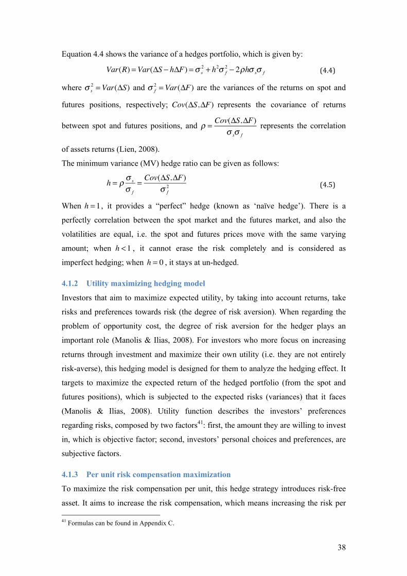
38

Equation 4.4 shows the variance of a hedges portfolio, which is given by:

Var(R) =Var(ΔS − hΔF) =σ s2 + h2σ f

2 − 2ρhσ sσ f (4.4)

where σ s2 =Var(ΔS) and σ f

2 =Var(ΔF) are the variances of the returns on spot and

futures positions, respectively; Cov(ΔS,ΔF) represents the covariance of returns

between spot and futures positions, and ρ = Cov(ΔS,ΔF)σ sσ f

represents the correlation

of assets returns (Lien, 2008).

The minimum variance (MV) hedge ratio can be given as follows:

h = ρ σ s

σ f

= Cov(ΔS,ΔF)σ f2 (4.5)

When h = 1 , it provides a “perfect” hedge (known as ‘naïve hedge’). There is a

perfectly correlation between the spot market and the futures market, and also the

volatilities are equal, i.e. the spot and futures prices move with the same varying

amount; when h <1 , it cannot erase the risk completely and is considered as

imperfect hedging; when h = 0 , it stays at un-hedged.

4.1.2 Utility maximizing hedging model

Investors that aim to maximize expected utility, by taking into account returns, take

risks and preferences towards risk (the degree of risk aversion). When regarding the

problem of opportunity cost, the degree of risk aversion for the hedger plays an

important role (Manolis & Ilias, 2008). For investors who more focus on increasing

returns through investment and maximize their own utility (i.e. they are not entirely

risk-averse), this hedging model is designed for them to analyze the hedging effect. It

targets to maximize the expected return of the hedged portfolio (from the spot and

futures positions), which is subjected to the expected risks (variances) that it faces

(Manolis & Ilias, 2008). Utility function describes the investors’ preferences

regarding risks, composed by two factors41: first, the amount they are willing to invest

in, which is objective factor; second, investors’ personal choices and preferences, are

subjective factors.

4.1.3 Per unit risk compensation maximization

To maximize the risk compensation per unit, this hedge strategy introduces risk-free

asset. It aims to increase the risk compensation, which means increasing the risk per 41 Formulas can be found in Appendix C.

39

unit can provide the more risk compensation of units. This model can make investors

with different risk appetites obtain their corresponding returns under different risk

levels42. Investors who dislike risks request a higher risk compensation per unit than

those who favor risks.

Comparing with former two methods, though unit risk compensation maximization

takes care of both risk and return, its calculation is complicated; and it introduces the

risk-free asset, this is not easy to be put into operation for investors. Besides, the

utility function for utility maximization hedging is difficult to construct accurately.

When facing different investors, the applied utility functions are not the same.

Through utility maximization model to determine the optimal hedge ratio, it does not

have the general meanings. The rear two of introduced three methods both have the

disadvantage of pre-determined the utility function, which is subjective to some extent.

Economics assumes that the rational investors are the investors who are risk-averse.

For them, the main purpose of hedging is to avoid risk of the spot market. The risk-

minimizing MVHR has a strong applicability. As a consequence, this thesis chooses

the risk-minimization model to do a further research.

4.2 Estimating hedging effectiveness based on risk-minimization hedging

model

4.2.1 Econometric models for hedging

• Model 1: OLS

This is the simplest model of the ordinary least squares (OLS) regression, which is a

linear regression of changes in spot prices on changes in futures prices. OLS

estimation of the following equation provides the best linear unbiased estimate of the

MVHR if the assumptions of the classical linear regression model hold (Jason Laws,

John Thompson, 2005).

The appropriate hedge ratio43 will be the slope estimate (i.e. β ) in a regression, where

the dependent variable is a time series of spot returns and the independent variable is

a time series of futures returns. The MV constant hedge ratio can be estimated from

the following expression:

ΔSt =α + βΔFt + ξt (4.6)

42 Formulas can be found in Appendix D. 43 The number of units of the futures asset to sell per unit of the spot asset held

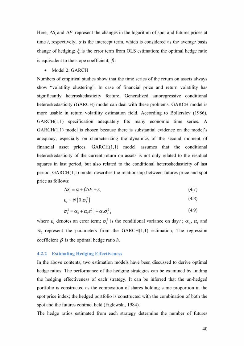
40

Here, ΔSt and ΔFt represent the changes in the logarithm of spot and futures prices at

time t, respectively; α is the intercept term, which is considered as the average basis

change of hedging; ξt is the error term from OLS estimation; the optimal hedge ratio

is equivalent to the slope coefficient, β .

• Model 2: GARCH

Numbers of empirical studies show that the time series of the return on assets always

show “volatility clustering”. In case of financial price and return volatility has

significantly heteroskedasticity feature. Generalized autoregressive conditional

heteroskedasticity (GARCH) model can deal with these problems. GARCH model is

more usable in return volatility estimation field. According to Bollerslev (1986),

GARCH(1,1) specification adequately fits many economic time series. A

GARCH(1,1) model is chosen because there is substantial evidence on the model’s

adequacy, especially on characterizing the dynamics of the second moment of

financial asset prices. GARCH(1,1) model assumes that the conditional

heteroskedasticity of the current return on assets is not only related to the residual

squares in last period, but also related to the conditional heteroskedasticity of last

period. GARCH(1,1) model describes the relationship between futures price and spot

price as follows:

ΔSt =α + βΔFt + ε t (4.7)

ε t ∼ N 0,σ t

2( )

(4.8)

σ t2 =α 0 +α1ε t−1

2 +α 2σ t−12

(4.9)

where ε t denotes an error term; σ t2 is the conditional variance on day t ; α 0 , α1 and

α 2 represent the parameters from the GARCH(1,1) estimation; The regression

coefficient β is the optimal hedge ratio h.

4.2.2 Estimating Hedging Effectiveness

In the above contents, two estimation models have been discussed to derive optimal

hedge ratios. The performance of the hedging strategies can be examined by finding

the hedging effectiveness of each strategy. It can be inferred that the un-hedged

portfolio is constructed as the composition of shares holding same proportion in the

spot price index; the hedged portfolio is constructed with the combination of both the

spot and the futures contract held (Figlewski, 1984).

The hedge ratios estimated from each strategy determine the number of futures

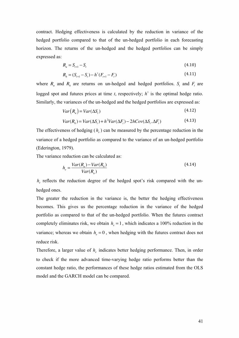
41

contract. Hedging effectiveness is calculated by the reduction in variance of the

hedged portfolio compared to that of the un-hedged portfolio in each forecasting

horizon. The returns of the un-hedged and the hedged portfolios can be simply

expressed as:

Ru = St+1 − St (4.10)

Rh = (St+1 − St )− h∗(Ft+1 − Ft )

(4.11)

where Ru and Rh are returns on un-hedged and hedged portfolios. St and Ft are

logged spot and futures prices at time t, respectively; h∗ is the optimal hedge ratio.

Similarly, the variances of the un-hedged and the hedged portfolios are expressed as:

Var Ru( ) =Var(ΔSt ) (4.12)

Var(Rh ) =Var(ΔSt )+ h2Var(ΔFt )− 2hCov(ΔSt ,ΔFt ) (4.13)

The effectiveness of hedging ( he ) can be measured by the percentage reduction in the

variance of a hedged portfolio as compared to the variance of an un-hedged portfolio

(Ederington, 1979).

The variance reduction can be calculated as:

he =Var(Ru )−Var(Rh )

Var(Ru )

(4.14)

he reflects the reduction degree of the hedged spot’s risk compared with the un-

hedged ones.

The greater the reduction in the variance is, the better the hedging effectiveness

becomes. This gives us the percentage reduction in the variance of the hedged

portfolio as compared to that of the un-hedged portfolio. When the futures contract

completely eliminates risk, we obtain he = 1 , which indicates a 100% reduction in the

variance; whereas we obtain he = 0 , when hedging with the futures contract does not

reduce risk.

Therefore, a larger value of he indicates better hedging performance. Then, in order

to check if the more advanced time-varying hedge ratio performs better than the

constant hedge ratio, the performances of these hedge ratios estimated from the OLS

model and the GARCH model can be compared.

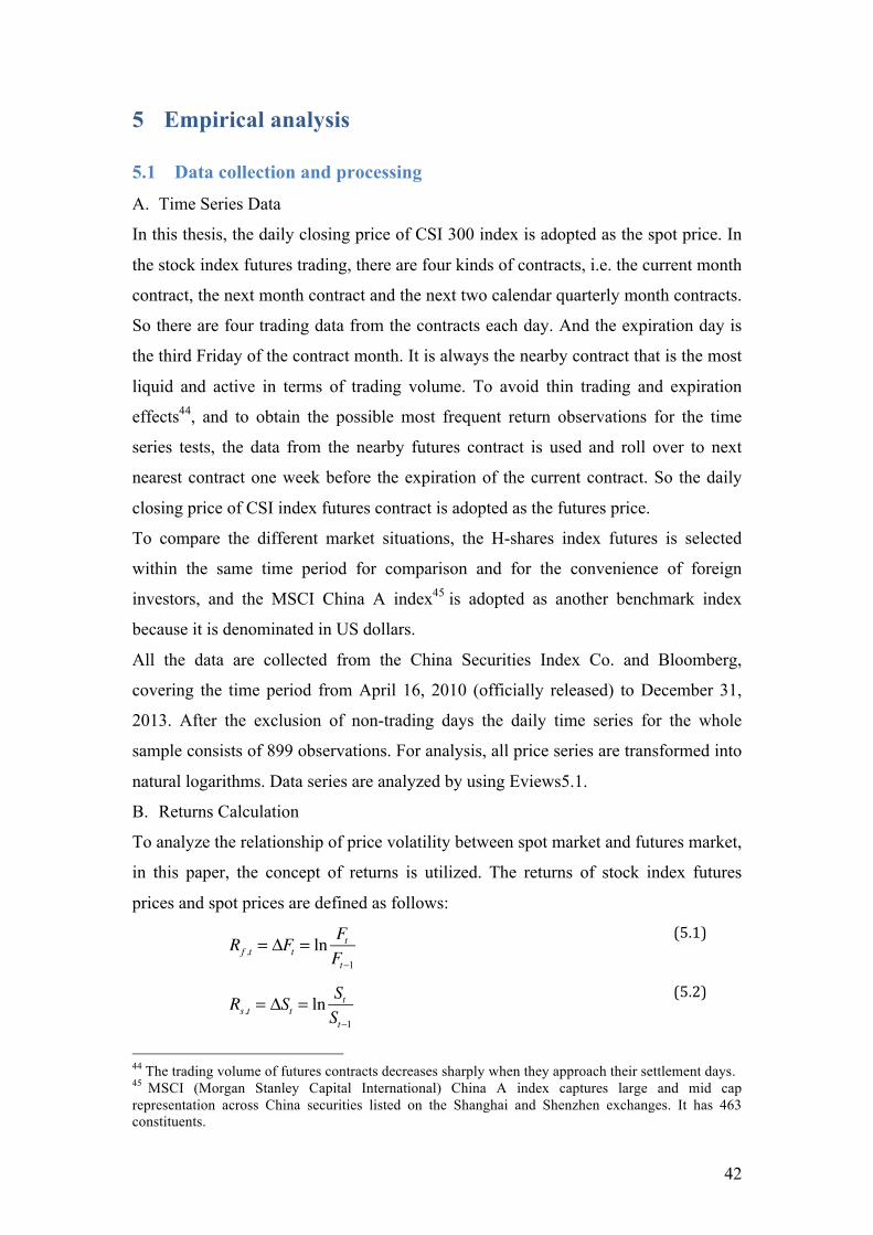
42

5 Empirical analysis

5.1 Data collection and processing A. Time Series Data

In this thesis, the daily closing price of CSI 300 index is adopted as the spot price. In

the stock index futures trading, there are four kinds of contracts, i.e. the current month

contract, the next month contract and the next two calendar quarterly month contracts.

So there are four trading data from the contracts each day. And the expiration day is

the third Friday of the contract month. It is always the nearby contract that is the most

liquid and active in terms of trading volume. To avoid thin trading and expiration

effects44, and to obtain the possible most frequent return observations for the time

series tests, the data from the nearby futures contract is used and roll over to next

nearest contract one week before the expiration of the current contract. So the daily

closing price of CSI index futures contract is adopted as the futures price.

To compare the different market situations, the H-shares index futures is selected

within the same time period for comparison and for the convenience of foreign

investors, and the MSCI China A index45 is adopted as another benchmark index

because it is denominated in US dollars.

All the data are collected from the China Securities Index Co. and Bloomberg,

covering the time period from April 16, 2010 (officially released) to December 31,

2013. After the exclusion of non-trading days the daily time series for the whole

sample consists of 899 observations. For analysis, all price series are transformed into

natural logarithms. Data series are analyzed by using Eviews5.1.

B. Returns Calculation

To analyze the relationship of price volatility between spot market and futures market,

in this paper, the concept of returns is utilized. The returns of stock index futures

prices and spot prices are defined as follows:

Rf ,t = ΔFt = ln

FtFt−1

(5.1)

Rs,t = ΔSt = ln

StSt−1

(5.2)

44 The trading volume of futures contracts decreases sharply when they approach their settlement days. 45 MSCI (Morgan Stanley Capital International) China A index captures large and mid cap representation across China securities listed on the Shanghai and Shenzhen exchanges. It has 463 constituents.

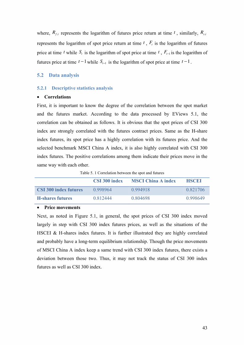
43

where, Rf ,t represents the logarithm of futures price return at time t , similarly, Rs,t

represents the logarithm of spot price return at time t , Ft is the logarithm of futures

price at time t while St is the logarithm of spot price at time t , Ft−1 is the logarithm of

futures price at time t −1while St−1 is the logarithm of spot price at time t −1 .

5.2 Data analysis

5.2.1 Descriptive statistics analysis

• Correlations

First, it is important to know the degree of the correlation between the spot market

and the futures market. According to the data processed by EViews 5.1, the

correlation can be obtained as follows. It is obvious that the spot prices of CSI 300

index are strongly correlated with the futures contract prices. Same as the H-share

index futures, its spot price has a highly correlation with its futures price. And the

selected benchmark MSCI China A index, it is also highly correlated with CSI 300

index futures. The positive correlations among them indicate their prices move in the

same way with each other. Table 5. 1 Correlation between the spot and futures

CSI 300 index   MSCI China A index   HSCEI  

CSI 300 index futures 0.998964 0.994918 0.821706

H-shares futures 0.812444 0.804698 0.998649

• Price movements

Next, as noted in Figure 5.1, in general, the spot prices of CSI 300 index moved

largely in step with CSI 300 index futures prices, as well as the situations of the

HSCEI & H-shares index futures. It is further illustrated they are highly correlated

and probably have a long-term equilibrium relationship. Though the price movements

of MSCI China A index keep a same trend with CSI 300 index futures, there exists a

deviation between those two. Thus, it may not track the status of CSI 300 index

futures as well as CSI 300 index.

44

Figure 5.1 Price movements of CSI 300 index and CSI 300 index futures

(From April 16, 2010 to Dec. 31, 2013)

Figure 5.2 MSCI China A index & CSI 300 index futures

Figure 5.3 HSCEI & H-shares futures

Note. Index futures prices ( lnF ) and spot index prices ( lnS ) are in logarithms.

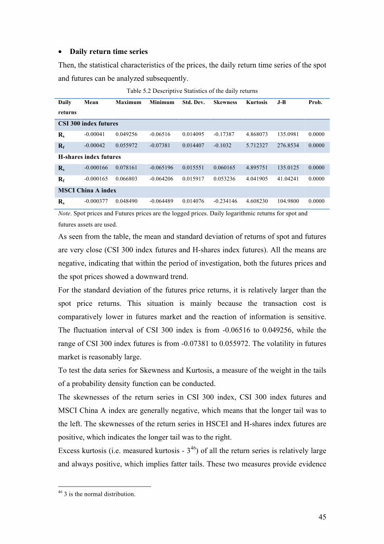
45

• Daily return time series

Then, the statistical characteristics of the prices, the daily return time series of the spot

and futures can be analyzed subsequently. Table 5.2 Descriptive Statistics of the daily returns

Daily

returns

Mean Maximum Minimum Std. Dev. Skewness Kurtosis J-B Prob.

CSI 300 index futures

Rs -0.00041 0.049256 -0.06516 0.014095 -0.17387 4.868073 135.0981 0.0000

Rf -0.00042 0.055972 -0.07381 0.014407 -0.1032 5.712327 276.8534 0.0000

H-shares index futures

Rs -0.000166 0.078161 -0.065196 0.015551 0.060165 4.895751 135.0125 0.0000

Rf -0.000165 0.066803 -0.064206 0.015917 0.053236 4.041905 41.04241 0.0000

MSCI China A index

Rs -0.000377 0.048490 -0.064489 0.014076 -0.234146 4.608230 104.9800 0.0000

Note. Spot prices and Futures prices are the logged prices. Daily logarithmic returns for spot and

futures assets are used.

As seen from the table, the mean and standard deviation of returns of spot and futures

are very close (CSI 300 index futures and H-shares index futures). All the means are

negative, indicating that within the period of investigation, both the futures prices and

the spot prices showed a downward trend.

For the standard deviation of the futures price returns, it is relatively larger than the

spot price returns. This situation is mainly because the transaction cost is

comparatively lower in futures market and the reaction of information is sensitive.

The fluctuation interval of CSI 300 index is from -0.06516 to 0.049256, while the

range of CSI 300 index futures is from -0.07381 to 0.055972. The volatility in futures

market is reasonably large.

To test the data series for Skewness and Kurtosis, a measure of the weight in the tails

of a probability density function can be conducted.

The skewnesses of the return series in CSI 300 index, CSI 300 index futures and

MSCI China A index are generally negative, which means that the longer tail was to

the left. The skewnesses of the return series in HSCEI and H-shares index futures are

positive, which indicates the longer tail was to the right.

Excess kurtosis (i.e. measured kurtosis - 346) of all the return series is relatively large

and always positive, which implies fatter tails. These two measures provide evidence

46 3 is the normal distribution.

46

that the all the return series are not normally distributed and have an obvious peak and

fat tails.

In addition, J-B statistic test are further proved that all the return series do not comply

with the normal distribution. Figures in the Appendix E show the histograms.

We can get the daily return fluctuation as shown in Figure 5.4, where the daily returns

of the index spot and index futures have a characteristic of volatility clustering. And

the futures prices is more volatile than the spot prices, which indicates the existence

of an arbitrage possibility. Figure 5.4 Line Graph of daily returns on CSI 300 index and CSI 300 index futures

5.2.2 Stationary test

Since, in most cases, the economic indicator series are non-stationary series. For the

estimation of optimal hedge ratio, using non-stationary data may lead to spurious

regressions and invalid conclusions (Cotter and Hanly, 2006).

In order to prevent false regression problems, it is desirable that the series involved

are stationary. Stationary means that the series will remain stable at different time

points, i.e., the mean and the covariance of a series are time-independent. To test for

stationarity, ADF unit root test47 is carried on each of the sample series. The results of

the series RS , RF are given in Table 5.3.

47 Augmented Dickey-Fuller (ADF) test is adopted.

47

Table 5.3 ADF test

Null Hypothesis: RS has a unit root

t-Statistic Prob.*

Augmented Dickey-Fuller test statistic -30.29874 0

Test critical values: 1% level -3.437418

5% level -2.864549

10% level -2.568426

Null Hypothesis: RF has a unit root

t-Statistic Prob.*

Augmented Dickey-Fuller test statistic -30.95061 0

Test critical values: 1% level -3.437418

5% level -2.864549

10% level -2.568426

Note. *MacKinnon (1996) one-sided p-values.

From the Table 5.3, it can be seen that the t-statistics of ADF test of RS and RF are

smaller than the critical values at 1% level, 5% level and 10% level. The two series in

the 1% significance level mean we can have at least about 99% confidence level to

reject the null hypothesis. So, the time series data do not have a unit root. In other

words, the series of daily returns shows that both of them are stable.

Application of the ADF test on the daily returns series of CSI 300 index and CSI 300

index futures indicates that both series are stationary at levels.

Then, similar tests can easily be applied on HSCEI, H-shares index futures and MSCI

China A index, the results shows that all three return series are stationary at levels48.

5.2.3 Cointegration test

Cointegration allows us to draw the reposeful relation between two or multiple series

(Gao, 2009). Sometimes, the time series are not stable themselves. But the linear

combination between different time series can be stationary.

The prerequisite for establishing hedge models is the existence of a long-term

equilibrium relationship between the variables. Therefore, it is necessary to run the

cointegration test of the variables. Johansen (1988) cointegration test are used here to

examine the spot and futures prices series.

48 Results are given in Appendix F.

48

Table 5.4 Johansen Cointegration Tests

Johansen cointegration test (trace statistics)

Hypothesized

No. of CE(s) Eigenvalue

Trace

Statistic

0.05

Critical Value Prob.**

r ≤ 0∗ 0.035494 35.82759 15.49471 0

r ≤1 0.003929 3.519401 3.841466 0.0606

Johansen co-integration test (max statistics)

Hypothesized

No. of CE(s) Eigenvalue

Max-Eigen

Statistic

0.05

Critical Value Prob.**

r ≤ 0∗ 0.035494 32.30819 14.2646 0

r ≤1 0.003929 3.519401 3.841466 0.0606

Note. Trace test indicates 1 co-integrating equation at the 0.05 level. Max-eigenvalue test indicates 1

co-integrating equation at the 0.05 level. *Denotes rejection of the hypothesis at the 0.05 level.

**MacKinnon-Haug-Michelis (1999) p-values.

Table 5.4 shows that both the trace statistics test and the maximum eigenvalue

statistics test reject the hypothesis of no-cointegration. The results suggest the

presence of one cointegrating vector between the spot and futures market prices at 5%

level respectively.

The Johansen test provides evidence that cash prices and futures prices series are co-

integrated for each case. The result implies that there is a well-defined long-run

relationship between the spot and futures prices.

Reasons for co-integration relationship

Why CSI 300 index and CSI 300 index futures have such a co-integration relationship?

One of main reasons is that CSI 300 index is designed as the underlying asset of the

stock index futures contracts. Therefore, the two subjects cannot be completely

divorced from each other. Although they may deviate from each other temporally,

caused by some economic factors, but the deviation will eventually disappear and

their prices trend will be the same.

So due to the existence of arbitrage, the index price will tend to perform in line with

the futures price eventually. If there exists irrational basis, then arbitrageurs can gain

the return of price spread through operating in a reverse direction in the two markets.

Similarly, either the index prices or the futures prices have the abnormal fluctuations,

speculators can benefit through related operations. The basic reason is that no matter

49

how the speculative action and arbitrage are conducted in the market, the supply and

demand can tend towards equilibrium, and the unreasonable price spread or basis will

tend to be reasonable until the market is unprofitable.

So it can be inferred that the futures price can be regarded as the spot price at a

particular moment in the future. With the approaching of the settlement date, the

position-holding cost of stock index futures will be gradually reduced and the price

spread between the cash and futures is getting narrow.

5.2.4 Summary

This section is mainly to prepare for the hedging model analysis. Based on above

arguments, the following conclusions can be obtained:

1) According to the statistical analysis, the CSI 300 index and the CSI 300 index

futures return series show the characteristics of non-normality, fat tail and

volatility clustering.

2) Based on the ADF test, it indicates that the return series of CSI 300 index futures

and spot are stationary time series. These results suggest that regressions can be

applied on the returns series.

3) The results of the co-integration analysis showed that there exists co-integration

relation between CSI 300 index futures price and CSI 300 index prices. Such a co-

integration correlation between the stock market and the futures market has laid

the foundation for the realization of hedging function. So we expect the CSI300

index futures to be an effective tool to hedge risk in spot market in China.

5.3 Hedging Model Analysis From the previous analysis, the CSI 300 index prices and CSI 300 index futures prices

have a strong correlation and exist a long-run equilibrium relationship. These features

provide the favored conditions for hedging by CSI 300 index futures.

In this section, the hedging effectiveness of CSI 300 index futures will be further

analyzed on the basis of the previous conclusions. Based on the universality and

continuity of data analysis, we assume that investors invest in the constituent stock of

the CSI 300 index and the ratios of stock share holdings are same as the weights of

the constituent stocks in the CSI 300 index (the same assumptions of investing in H-

shares index futures and MSCI China A index). Here, different econometric models

are adopted to calculate the hedge ratios and hedging effectiveness. And the results

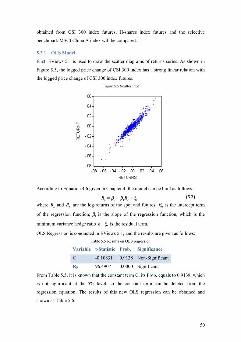
50

obtained from CSI 300 index futures, H-shares index futures and the selective

benchmark MSCI China A index will be compared.

5.3.1 OLS Model

First, EViews 5.1 is used to draw the scatter diagrams of returns series. As shown in

Figure 5.5, the logged price change of CSI 300 index has a strong linear relation with

the logged price change of CSI 300 index futures. Figure 5.5 Scatter Plot

According to Equation 4.6 given in Chapter.4, the model can be built as follows:

(5.3)

where RS and RF are the log-returns of the spot and futures; β0 is the intercept term

of the regression function; β1 is the slope of the regression function, which is the

minimum variance hedge ratio h ; ξt is the residual term.

OLS Regression is conducted in EViews 5.1, and the results are given as follows: Table 5.5 Results on OLS regression

Variable t-Statistic Prob. Significance

C -0.10831 0.9138 Non-Significant

RF 96.4907 0.0000 Significant

From Table 5.5, it is known that the constant term C, its Prob. equals to 0.9138, which

is not significant at the 5% level, so the constant term can be deleted from the

regression equation. The results of this new OLS regression can be obtained and

shown as Table 5.6:

RS = β0 + β1RF + ξt

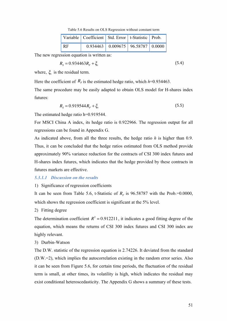
51

Table 5.6 Results on OLS Regression without constant term

Variable Coefficient Std. Error t-Statistic Prob.

RF 0.934463 0.009675 96.58787 0.0000

The new regression equation is written as:

RS = 0.934463RF + ξt (5.4)

where, ξt is the residual term.

Here the coefficient of RF is the estimated hedge ratio, which h=0.934463.

The same procedure may be easily adapted to obtain OLS model for H-shares index

futures:

RS = 0.919544RF + ξt (5.5)

The estimated hedge ratio h=0.919544.

For MSCI China A index, its hedge ratio is 0.922966. The regression output for all

regressions can be found in Appendix G.

As indicated above, from all the three results, the hedge ratio h is higher than 0.9.

Thus, it can be concluded that the hedge ratios estimated from OLS method provide

approximately 90% variance reduction for the contracts of CSI 300 index futures and

H-shares index futures, which indicates that the hedge provided by these contracts in

futures markets are effective.

5.3.1.1 Discussion on the results

1) Significance of regression coefficients

It can be seen from Table 5.6, t-Statistic of RF is 96.58787 with the Prob.=0.0000,

which shows the regression coefficient is significant at the 5% level.

2) Fitting degree

The determination coefficient R2 = 0.912211 , it indicates a good fitting degree of the

equation, which means the returns of CSI 300 index futures and CSI 300 index are

highly relevant.

3) Durbin-Watson

The D.W. statistic of the regression equation is 2.74226. It deviated from the standard

(D.W.=2), which implies the autocorrelation existing in the random error series. Also

it can be seen from Figure 5.6, for certain time periods, the fluctuation of the residual

term is small, at other times, its volatility is high, which indicates the residual may

exist conditional heteroscedasticity. The Appendix G shows a summary of these tests.

52

Figure 5.6 Trend of the random errors for RS

5.3.1.2 Test OLS residual

Then, the test of the heteroscedasticity is required on the random error sequence of the

linear regression. If the serial data of the random errors have obvious

heteroscedasticity phenomena, then the GARCH model should be used to calculate

the hedge ratio.

The results of ARCH LM test are shown as below: Table 5.7 results on Residual test

ARCH Test:

F-statistic 30.48008 Prob. F(1,895) 0.0000

Obs*R-squared 29.5421 Prob. Chi-Square(1) 0.0000

The Table shows that F-statistic=30.48008, Probability=0.0000, which means the F-

statistic reject the null hypothesis; LM statistics Obs*R-squared=29.5421, the

distribution probability of χ 2 is 0, clearly less than the 5% significance level. All of

these indicate that there exists the ARCH effect in the random error sequence of the

regression equation.

The results of OLS model imply that there are auto-correlations and ARCH effect of

the random error sequence, which would affect the validity of OLS model. Therefore,

the GARCH model is introduced to estimate the hedging ratio.

5.3.2 GARCH Model

According to the equations in Chapter 4, the results are given as follow by using

EViews 5.1:

53

Table 5.8 Results on GARCH(1,1) Regression

Coefficient Std. Error z-Statistic Prob.

C 2.01E-05 0.000119 0.169236 0.8656

RF 0.953208 0.008036 118.6189 0.0000

In which, the z-Statistic of the constant term C is 0.169236, Prob.=0.8656. It is found

to be insignificant at the 5% level, which cannot explain the regression equation well.

It was therefore excluded from the final estimations.

Then the model is written as: RS = βRF + ξt .

Based on the new model, the new results on GARCH(1,1) regression is shown in table

below: Table 5.9 Results on GARCH(1,1) Regression (without constant term)

Coefficient Std. Error z-Statistic Prob.

RF 0.953181 0.008039 118.5769 0.0000

C 1.81E-06 6.36E-07 2.840641 0.0045

RESID(-1)^2 0.113521 0.027379 4.146245 0

GARCH(-1) 0.782801 0.054495 14.36471 0

The GARCH(1,1) model is written as:

RS = 0.953181RF + ξt (5.6)

σ t2 = 1.81×10−6 + 0.113521ξt−1

2 + 0.782801σ t−12 (5.7)

where the coefficient of RF is the estimated hedge ratio of CSI 300 index futures, that

h=0.953181.

The model of H-shares futures is:

RS = 0.930577RF Its hedge ratio h is 0.930577.

When using MSCI China A index as benchmark, its hedge ratio h is 0.943561. Tables

in Appendix H show the results for all the regressions.

5.3.2.1 Discussion on the results49

1) Significance of regression coefficients

It can be seen from above table, the probability of z-Statistic is 0, which means the

regression coefficient of RF is significant at the 5% level.

49 Results are shown in Appendix H.

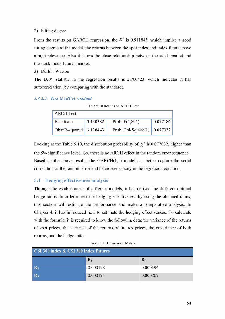
54

2) Fitting degree

From the results on GARCH regression, the R2 is 0.911845, which implies a good

fitting degree of the model, the returns between the spot index and index futures have

a high relevance. Also it shows the close relationship between the stock market and

the stock index futures market.

3) Durbin-Watson

The D.W. statistic in the regression results is 2.760423, which indicates it has

autocorrelation (by comparing with the standard).

5.3.2.2 Test GARCH residual Table 5.10 Results on ARCH Test

ARCH Test:

F-statistic 3.130382 Prob. F(1,895) 0.077186

Obs*R-squared 3.126443 Prob. Chi-Square(1) 0.077032

Looking at the Table 5.10, the distribution probability of χ 2 is 0.077032, higher than

the 5% significance level. So, there is no ARCH effect in the random error sequence.

Based on the above results, the GARCH(1,1) model can better capture the serial

correlation of the random error and heteroscedasticity in the regression equation.

5.4 Hedging effectiveness analysis Through the establishment of different models, it has derived the different optimal

hedge ratios. In order to test the hedging effectiveness by using the obtained ratios,

this section will estimate the performance and make a comparative analysis. In

Chapter 4, it has introduced how to estimate the hedging effectiveness. To calculate

with the formula, it is required to know the following data: the variance of the returns

of spot prices, the variance of the returns of futures prices, the covariance of both

returns, and the hedge ratio. Table 5.11 Covariance Matrix

CSI 300 index & CSI 300 index futures

RS RF

RS 0.000198 0.000194

RF 0.000194 0.000207

55

As the table shows, the variances of CSI 300 index and its futures can be obtained:

Var(RU ) = 0.000198 , Var(RH ) = 0.000207 , Cov(RS ,RF ) = 0.000194 .

According to the Equation of he , the results appear by computation as shown below:

Table 5.12 Results on hedging effectiveness

Criteria OLS GARCH

CSI 300 index futures

h 0.934463 0.953181

Var(RU) 0.000198 0.000198

Var(RH) 1.61851E-05 1.62365E-05

he 0.918256953 0.917997708

H-shares50

h 0.919544 0.930577

he 0.886601542 0.886696399

MSCI China A index51

h 0.922966 0.943561

he 0.890084348 0.889629689

As seen in the above table, compared to the variance of returns in an unhedged

position, the results in a hedged position have drastically reduced by using CSI 300

index futures. Both models can decrease the systematic risk efficiently. It also reveals

that the optimal hedge ratios estimated from GARCH model are slightly larger than

those estimated from OLS model for both index futures markets. The dynamic hedge

ratio h=953181 based on GARCH model is better than the static hedge ratio

h=0.934463 based on OLS model.

From the view of the effect of risk aversion, CSI 300 index futures indicates higher

hedging effectiveness. It is shown that the hedging effectiveness of CSI 300 index

futures (0.917997708) was higher than that of H-shares index futures (0.886696399).

It is also shown that CSI 300 index futures provides more effective hedge for the two

hedge ratio estimation models compared to H-shares index futures.

The results also indicate that OLS model performs more effectively in Chinese index

futures market. But one of the basic assumptions of OLS model is that the financial

time series have the same variance. However, GARCH model dose not have such

50 The results are provided in Appendix I. 51 The results are provided in Appendix I.

56

assumptions. It can be applied to the case that financial time series have

heteroscedasticity. Theoretically, GARCH model has a strong applicability of related

analysis in the financial markets and using this model to estimate the hedge ratio is

better.

In general, the hedging effectiveness for index futures using different models is above

90%, which indicates that the index futures can help investors to hedge risk in spot

market to a large extent. In this case, CSI 300 index futures contracts can be

suggested as effective tool for hedging risk.

57

6 Conclusion and perspective The purpose of this study is to explore the impact of the introduction of stock index

futures on Chinese stock market, and empirically test the CSI 300 index futures.

6.1 Conclusion

At the beginning of this study, it outlines the basic theory of stock index futures and

hedging, and briefly describes the development of Chinese stock index futures

market. From the perspective of the development, CSI 300 index future has

maintained a steady growth during its initial of operation in China. Then, by selecting

the transaction data in the market, processing and analyzing them empirically, the

correlation between CSI 300 index futures and spot index has been verified. Two tests,

i.e. the stationarity test and cointegration test, have been mainly adopted during the

verification. Thereafter, the two commonly used models (OLS and GARCH) are

introduced to estimate the optimal hedge ratio, and the hedging effectiveness of CSI

300 index futures are analyzed and evaluated at the same time. Taken together, the

following conclusions have been made:

1) Results from the stationarity test and the cointegration test

The logarithm price series of CSI 300 spot and futures are stationary at the first order

difference, which means both returns series are stationary time series.

Then, this paper confirms the existence of a long-term equilibrium relationship

between the CSI 300 index and index futures through the co-integration test. This

conclusion demonstrates the existence of co-movement between the stock market and

the stock index futures market. For the further explanation, it is that the prices in two

markets influence each other and the fluctuant prices will show a convergence trend

eventually. This long-term equilibrium relationship provides a prerequisite for

hedging.

Meanwhile, the stock index futures prices have been more volatile than the spot

prices. Consequently, there exists arbitrage space in the market price, which indicates

the risk-averse ability of stock index futures need to be further strengthened.

2) Hedge ratio and Hedging effectiveness

In order to evaluate the efficiency of hedge, the determination of the optimal hedge

ratio is firstly required, and OLS method and GARCH(1,1) model are both adopted.

Through the calculation by EViews, the estimated hedge ratio based on GARCH

model is 0.953181, which is slightly higher than 0.934463 obtained from OLS model.

58

Both ratios are close to perfect hedge (h = 1 ). The hedging effectiveness of the two

models is around 0.92, which indicates the CSI 300 index futures can hedge 92% risk

of the spot. The results in this study show that the error term of OLS is auto-correlated

and has ARCH effect. So OLS model cannot accurately analyze the hedge effect of

CSI 300 index futures, but GARCH(1,1) model can overcome the limitations of the

traditional method of OLS. GARCH model can provide a more accurate analysis of

the hedge effect of stock index futures, where the hedge ratio is 0.953181 and the

hedging effectiveness is 0.917998. Through the comparison analysis between CSI 300

index futures and H-shares index futures, CSI 300 index futures is more efficient than

H-shares index futures. And CSI 300 index is more correlated with CSI 300 index

futures than MSCI China A index. To choose the benchmark as indicating hedging

effect, the stock portfolio should be better built to effectively track the CSI 300 index

trend.

In conclusion, the evaluation results support the view that the CSI 300 index futures

provides investors with better risk-management tool. CSI 300 index futures have a

great hedge effect. Hedge by using CSI 300 index futures can effectively reduce risks

and ensure the stability of returns. However, when choosing a specific hedging model,

it takes into account the characteristics of the underlying asset and the investors’ risk

tolerance, thus it is able to get the most satisfactory hedge effect.

6.2 Suggestions for investors

Based on the above analysis and discussion in this thesis, some suggestions can be

given to investors:

1) Selection of the hedged underlying

When investors chose the hedged underlying, the stock portfolio should be highly

correlated with the futures’ underlying, and the holding period of futures contracts

needs to correspond to the same period of risk-taking in the stock market. Only high

correlation between the spot asset and the CSI 300 index futures can ensure a great

hedge effect. Although the basis will tend to be 0 as the settlement date approaches, if

the hedging period is inconsistent with the delivery day, the basis risk still appears.

Therefore, investors should make the hedging period remain the same or close to the

futures contract maturity date.

2) Selection of the hedging model

59

The selection of model for estimating hedge ratio has been already analyzed. In

practice, investors should note that they could accurately estimate the optimal hedge

ratio by choosing a different model depending on the market conditions and their

investment preferences. In this paper, in order to choose the model, it is assumed the

investor is risk averse and wants to achieve risk minimization. If the investors who

favor risks, the conclusions through empirical analysis of this study are not applied to

them. Those investors should use other premise, such as expected utility

maximization.

In general, if the market is volatile, for long-term hedging operations, it is suggested

to use GARCH model or OLS model to estimate the optimal hedge ratio. Although

OLS model has the stringent assumptions, it is still very widely applied in practice.

For long-term hedge, investors also need to timely adjust the hedge ratio and the

positions structure of the portfolio according to the change of market conditions, in

order to improve the efficiency of hedging and reduce the risk of portfolios.

6.3 Limitations and future work

In this paper, during the analysis of hedging effectiveness of CSI 300 index futures,

there are still several shortages, which need to be further improved and perfected.

1) The scope of the study

Since the introduction time of CSI 300 index futures is short, there is a limited amount

of collected data. In the empirical analysis of this study, it has drawbacks of

insufficient sample data and short time period, so the conclusions may not be

generally applicable. In the actual situation, the market is closed on holidays. So the

data is non-continuous, which makes the advantages of GARCH model cannot be

fully achieved. Also, size of the sample will affect the accuracy of the empirical

results.

The stock market is constantly changing. The daily frequency data can better

characterize the trading behavior of investors and the trading changes. For further

work, based on the research of daily closing prices of stock index futures, it should

more carefully study the data change trends per hour or per minute intraday, estimate

the hedge effect in a short time, and draw the appropriate conclusions.

This paper studies the hedging effects of CSI 300 index futures, mainly from the view

on macroscopic. It did not give specific investment programs for particular investors.

They can replicate the movement of CSI 300 index through invest in stock portfolio

60

and use the hedge ratio obtained from this paper, to achieve an effective risk

management.

2) The determination of hedging models

In the aspect of model determination, it did not take into account the transaction costs,

the market impact costs and the opportunity costs, which can affect the hedge ratios.

The hedging performance is sure to be affected accordingly. In this study, it is based

on ideal conditions, which has the prerequisite of sufficient capital, no time and

money consuming of adjusting positions. While in the real investment, it needs to

consider the increased cost caused by adjustment positions, time consuming and many

other factors, which can further impact the hedging model choice of investors. To

improve the model, the cost factor should be considered as a variable in it. In addition,

different investors have different risk preferences. It should carefully consider the

hedgers’ expected returns and risk preferences, and set the related risk preference

coefficient, which makes the model can reflect risk tolerance of different investors.

3) Margin management

During the process of hedging, investors also need to concern the risks of the

variation margin and mark-to-market. Due to the implementation of the margin and

the daily settlement system in stock index futures trading, once an unfavorable change

happened in the futures market, its equity may fall below the minimum margin

maintenance and the investor will receive a margin call. If investors cannot be able to

make up the margin, the Exchange will execute mandatory liquidation for under-

margin positions. Accordingly, investors should fully estimate the number of margin

and prepare money for a rainy day.

61

Reference Book

Blank, Steven C., Carter, Colin A., and Schmiesing, Brian H. (1991), Futures and options

markets: Trading in commodities and financials, Prentice Hall.

Bodie, Zvi; Kane, Alex; Marcus, Alan J. (2011), Investments and portfolio management,

McGraw-Hill.

Chance, Don M. and Brooks, Robert (2008), An introduction to derivatives and risk

management, Thomson.

Cusatis, Patrick and Thomas, Martin (2005), Hedging Instruments and Risk Management,

McGraw-Hill Education.

David A. Dubofsky & Thomas W. Miller, Jr. (2003), Derivatives: valuation and risk

management, Oxford University Press, Inc.

Daigler, Robert T. (1993), Financial futures markets, concepts, evidence and applications,

HarperCollins College Publishers.

Hull, John C. (2011), Fundamentals of futures and options markets, Prentice Hall.

Hull, John C. (2012), Options, Futures, and other derivatives, Pearson.

Kolb, Robert W. (2003), Futures, options, and swaps, Blackwell Publishers.

Kolb, Robert W. (1999), Understanding futures markets, Blackwell.

Koziol, Joseph D. (1990), Hedging, principles, practice and strategies for the financial

markets, Wiler.

Robert E. Whaley (2006), Derivatives: Markets, Valuation, and Risk Management, John

Wiley & Sons, Inc.

Schwarz, Edward W., Hill, Joanne M., and Schneeweis, Thomas (1986), Financial futures,

fundanmentals, strategies, and applications. Homewood, ill.

Sutcliffe, Charles M.S. (1993), Stock index futures, theories and international evidence,

Chapmann&Hall.

Tiemei, Gao (2009), Econometrics analysis and modeling: application and example in

Eviews. Tsinghua University press.

Zhang Peter G. & Chan, Thomas. (2011), The Chinese Yuan: Internationalization and

Financial Products in China, John Wiley & Sons.

Gregoriou, Greg N., Kooli, Maher (2011), Hedge fund replication, Palgrave Macmillan.

Journal

Antoniou A and Holmes P, “Futures Trading, Information and Spot Price Volatility: Evidence

for the FTSE-100 Stock Index Futures Contract Using GARCH”. Journal of Banking &

Finance, 1995, Vol.19, PP. 117-129.

62

Besserrlbinder, Hendri and Paul J. Seguin, “Futures-Trading Activity and Stock Price

Volatility”. Journal of Finance, 1992, 47, 2015-2034.

Bollerslev T., “Generalized Autoregressive Conditional Heteroskedasticity”. Journal of

Econometircs, 1986, 307-327．

Cecchetti, S. G., Cumby, R. E., and Figlewski, S., “Estimation of the optimal futures hedge”.

Review of Economics and Statistics, 1988, 70, 623-630.

Carol Alexander and Andreza Barbosa, “Effectiveness of Minimum-Variance Hedging”. The

Journal of Portfolio Management, winter 2007.

Cotter, J. and Hanly, J., “Revaluating Hedging Performance”. The Journal of Futures

Markets, 26(7), 2006, 677–702.

D. Lien and K. Shrestha, “Hedging effectiveness comparisons: A note”. International Review

of Economics and Finance, 17(2008) 391-396.

Ederington L H., “The hedging performance of the new futures markets”. Journal of Finance,

1979, 34:157-170.

Edwards. F., “Does the futures trading increase stock market volatility”. Financial Analysts

Journal, 1988(44): 63-69.

Engle, R. F, “Autoregressive Conditional Heteroskedasticity with Estimates of the Variance

of UK inflation”, Econometrica. Vol.50, PP. 987-1008, 1982.

Gagnon, L., and Lypny, G., “Hedging shtor-term interest risk under time-varying

distributions”. Journal of Futures Markets, 1995, 15, 767-783.

Gray, R. W. and Rutledge, David J. S., “The Economics of Commodity Futures Markets: A

Survey”, Review of Marketing and Agricultural Economics, 39(1971): 57-108.

Huseyin Gulen and Stewartrt Mayhew, “Stock Index Futures Trading and Volatility in

International Equity Market”. The Journal of Futures Markets. 2000. Vol.20, No. 7: 661-685.

Jason Laws and John Thompson, “Hedging effectiveness of stock index futures”. European

Journal of Operational Research, 163(2005) 177-191.

Johnson L. L., “The theory of hedging and speculation in commodity futures”. Review of

Economic Studies, 1960, 27(3):139-151.

Kroner, K F., and Sultan, J., “Time-varying distributions and dynamic hedging with foreign

currency futures”. Journal of Financial and Quantitative Analysis, 1993, 28, 535-551.

Lawrence Harris. “S&P500 Cash Stock Price Volatilities”. The Journal of Finance, 1989(5):

1155-1117.

Lee S.B. and Ohk K.Y., “Stock Index Futures Listing Structural Change in Time Varying

Volatility”. Journal of Futures Markets, 1992, 12, 493-509.

Lien, D. and Luo, X., “Estimating multi-period hedge ratios in cointegrated markets”. Journal

of Futures Markets, 1994, (13): 909-920.

63

Lien, D., “The Effect of the Cointegration Relationship on Futures Hedging: a Note”, Journal

of Futures Markets, 1996.

Lien, D., Tse, T. K., Tsui Albert, K. C., “Evaluating the Hedging Performance of the

Constant-Correlation GARCH Model”, Applied Financial Economics, Vol.12, PP. 791-798,

2002.

Manolis G. Kavussanos & Ilias D. Visvikis, “Hedging effectiveness of the Athens stock index

futures contracts”. The European Journal of Finance, 2008, 14:3, 243-270.

Park, T. H, and Switzer, L. N., “Bivariate—GARCH estimation of the optimal hedge ratios

for stock index futures: A note”. Journal of Futures Markets, 1995, 15, 61-67.

Salil K Sarkar and Niranjan Tripathy, “An empirical analysis of the impact of stock index

futures trading on securities dealers’ inventory risk in the NASDAQ market Finance and Real

Estate Department”. University of North Texas, Denton, USA, 2002:13-19.

S. Figlewski, “Hedging Performance and Basis Risk in Stock Index Futures”. The Journal of

Finance, Vol. 39, No. 3, pp. 657-669, 1984.

Shu Y. Ma, “China’s privatization, from gradualism to shock therapy?” Asian Survey, 2008,

Vol. 48, No.2, pp. 199-214.

Wahab, M., Lashgari, M., “Price Dynamics and Error Correction in Stock Index and Stock

Index Futures Markets: a Cointegration Approach”, Journal of Futures Markets, 1993.

Working, H., “Speculation on hedging markets”. Food Research Institute Studies, 1960, (1)2.

pp. 185-220.

Xiaoxiong Fang, “Competitive analysis between CSI 300 index futures and overseas China

Concept index futures”, New Finance (in Chinese), 2008(2)

Xiya Luo, “Study on the financing methods of China’s listed companies”, the 3rd

International Conference on Information and Financial Engineering, IPEDR, Vol.12 (2011).

Yongwei Chen & Dong Li, “RMB Appreciation, Output Growth, and Inflation”, Economic

and Political Studies, Vol.1, No. 2, 2013, 3-17.

Editorial Board, China Stock Market Handbook, Javvin Press, 2008.

OECD (2011), Corporate Governance of Listed Companies in China: Self-Assessment by the

China Securities Regulatory Commission, OECD Publishing.

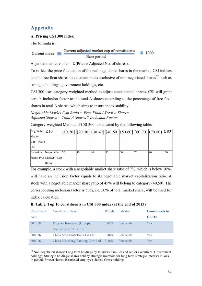
64

Appendix A. Pricing CSI 300 index

The formula is:

Adjusted market value = Σ (Price× Adjusted No. of shares).

To reflect the price fluctuation of the real negotiable shares in the market, CSI indices

adopts free float shares to calculate index exclusive of non-negotiated shares52 such as

strategic holdings, government holdings, etc.

CSI 300 uses category-weighted method to adjust constituents’ shares. CSI will grant

certain inclusion factor to the total A shares according to the percentage of free float

shares in total A shares, which aims to insure index stability.

Negotiable Market Cap Ratio = Free Float / Total A Shares Adjusted Shares = Total A Shares * Inclusion Factor

Category-weighted Method of CSI 300 is indicated by the following table: Negotiable

Market

Cap Ratio

(%)

≤10 10,20( ] 20,30( ] 30,40( ] 40,50( ] 50,60( ] 60,70( ) 70,80( ) ≥ 80

Inclusion

Factor (%)

Negotiable

Market Cap

Ratio

20 30 40 50 60 70 80 100

For example, a stock with a negotiable market share ratio of 7%, which is below 10%,

will have an inclusion factor equals to its negotiable market capitalization ratio. A

stock with a negotiable market share ratio of 45% will belong to category (40,50]. The

corresponding inclusion factor is 50%, i.e. 50% of total market share, will be used for

index calculation.

B. Table. Top 10 constituents in CSI 300 index (at the end of 2013) Constituent

code

Constituent Name Weight Industry Constituents in

HSCEI

601318 Ping An Insurance (Group)

Company of China Ltd

3.85% Financials Yes

600036 China Merchants Bank Co Ltd 3.46% Financials Yes

600016 China Minsheng Banking Corp Ltd 3.36% Financials Yes

52 Non-negotiated shares: Long term holdings by founders, families and senior executives; Government holdings; Strategic holdings: shares held by strategic investors for long-term strategic interests in lock-in period; Frozen shares; Restricted employee shares; Cross holdings

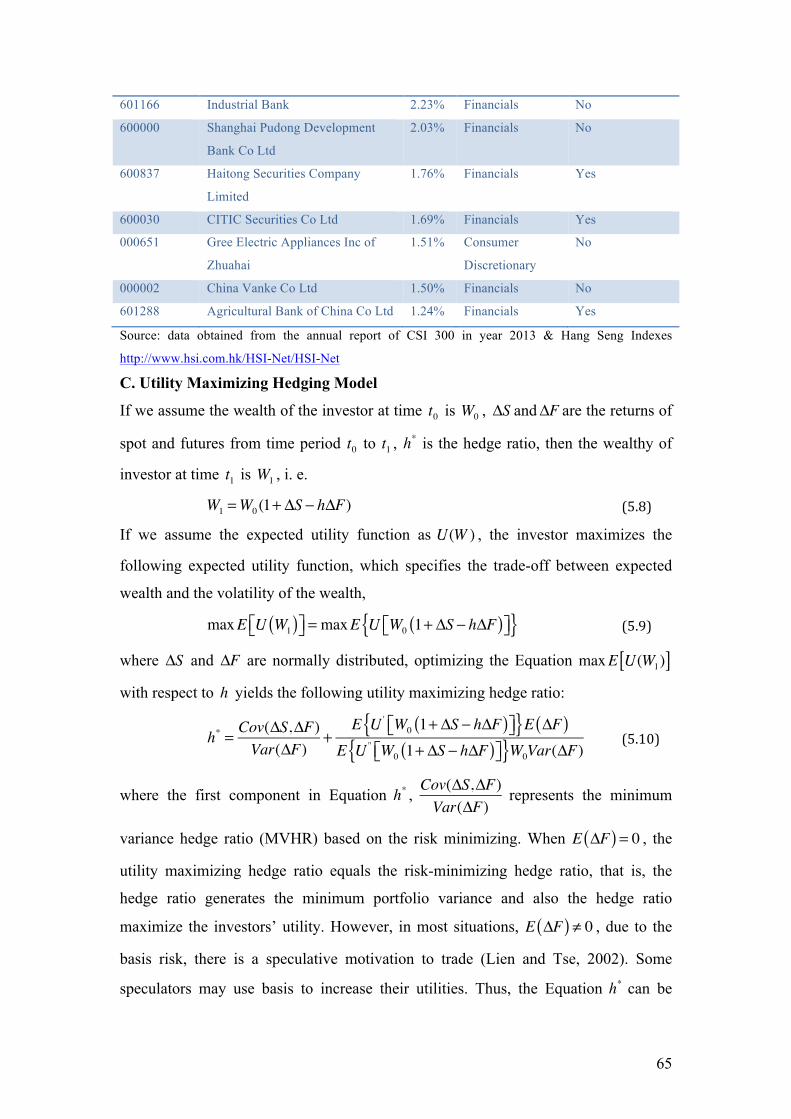
65

601166 Industrial Bank 2.23% Financials No

600000 Shanghai Pudong Development

Bank Co Ltd

2.03% Financials No

600837 Haitong Securities Company

Limited

1.76% Financials Yes

600030 CITIC Securities Co Ltd 1.69% Financials Yes

000651 Gree Electric Appliances Inc of

Zhuahai

1.51% Consumer

Discretionary

No

000002 China Vanke Co Ltd 1.50% Financials No

601288 Agricultural Bank of China Co Ltd 1.24% Financials Yes

Source: data obtained from the annual report of CSI 300 in year 2013 & Hang Seng Indexes

http://www.hsi.com.hk/HSI-Net/HSI-Net

C. Utility Maximizing Hedging Model

If we assume the wealth of the investor at time t0 is W0 , ΔS andΔF are the returns of

spot and futures from time period t0 to t1 , h* is the hedge ratio, then the wealthy of

investor at time t1 is W1 , i. e.

W1 =W0 (1+ ΔS − hΔF) (5.8)

If we assume the expected utility function as U(W ) , the investor maximizes the

following expected utility function, which specifies the trade-off between expected

wealth and the volatility of the wealth,

maxE U W1( )⎡⎣ ⎤⎦ = maxE U W0 1+ ΔS − hΔF( )⎡⎣ ⎤⎦{ } (5.9)

where ΔS and ΔF are normally distributed, optimizing the Equation maxE U(W1)[ ] with respect to h yields the following utility maximizing hedge ratio:

h* = Cov(ΔS,ΔF)

Var(ΔF)+

E U ' W0 1+ ΔS − hΔF( )⎡⎣ ⎤⎦{ }E ΔF( )E U '' W0 1+ ΔS − hΔF( )⎡⎣ ⎤⎦{ }W0Var(ΔF)

(5.10)

where the first component in Equation h* , Cov(ΔS,ΔF)Var(ΔF)

represents the minimum

variance hedge ratio (MVHR) based on the risk minimizing. When E ΔF( ) = 0 , the

utility maximizing hedge ratio equals the risk-minimizing hedge ratio, that is, the

hedge ratio generates the minimum portfolio variance and also the hedge ratio

maximize the investors’ utility. However, in most situations, E ΔF( ) ≠ 0 , due to the

basis risk, there is a speculative motivation to trade (Lien and Tse, 2002). Some

speculators may use basis to increase their utilities. Thus, the Equation h* can be

66

distinguished as two components: the first part is the MVHR, whereas the second one

represents the speculative component.

D. Per Unit Risk Compensation Maximization Model

In the investment portfolio, it includes spot asset, futures asset and risk-free asset. We

assume the risk-free return rate is rf , Ri represents the yield of portfolio i , σ i is the

standard deviation of Ri , in order to obtain the risk compensation per unit

maximization, it must make max E Ri( )− rfσ i

true. To get the optimal hedge ratio:

h =

E Rf( )− rf⎡⎣ ⎤⎦σ s2 − ρσ sσ f E(Rs )− rf⎡⎣ ⎤⎦

E(Rs )− rf⎡⎣ ⎤⎦σ f2 − ρσ sσ f E(Rf )− rf⎡⎣ ⎤⎦

= λ − ρ1− λρ( )π (5.11)

where, λ =E(Rf )− rf⎡⎣ ⎤⎦ σ f

E(Rs )− rf⎡⎣ ⎤⎦ σ s

,π =σ f

σ s

.

E. Descriptive statistics (histogram statistics) on return serials

• CSI 300 index & CSI 300 index futures

• HSCEI & H-shares index futures

67

• MSCI China A index

F. ADF test results

• HSCEI

Null Hypothesis: HKRS has a unit root Exogenous: Constant Lag Length: 0 (Automatic based on SIC, MAXLAG=20) t-Statistic Prob.* Augmented Dickey-Fuller test statistic -29.99425 0 Test critical values: 1% level

5% level 10% level

-3.437418 -2.864549 -2.568426

• H-shares index futures

Null Hypothesis: HKRF has a unit root Exogenous: Constant Lag Length: 0 (Automatic based on SIC, MAXLAG=20) t-Statistic Prob.* Augmented Dickey-Fuller test statistic -30.32618 0 Test critical values: 1% level

5% level 10% level

-3.437418 -2.864549 -2.568426

• MSCI China A index

Null Hypothesis: MSCIRS has a unit root Exogenous: Constant Lag Length: 0 (Automatic based on SIC, MAXLAG=20) t-Statistic Prob.* Augmented Dickey-Fuller test statistic -30.01222 0 Test critical values: 1% level

5% level 10% level

-3.437418 -2.864549 -2.568426

68

G. Results for OLS regression

• CSI 300 index & CSI 300 index futures

Dependent Variable: RETURNS Method: Least Squares Date: 05/03/14 Time: 13:01 Sample (adjusted): 1 898 Included observations: 898 after adjustments

Variable Coefficient Std. Error t-Statistic Prob. RETURNF 0.934463 0.009675 96.58787 0

R-squared 0.912211 Mean dependent var -0.000406 Adjusted R-squared 0.912211 S.D. dependent var 0.014095 S.E. of regression 0.004176 Akaike info criterion -8.117675 Sum squared resid 0.015645 Schwarz criterion -8.112329 Log likelihood 3645.836 Durbin-Watson stat 2.74226

• HSCEI & H-shares index futures

Dependent Variable: HKRS Method: Least Squares Date: 05/12/14 Time: 21:48 Sample (adjusted): 1 898 Included observations: 898 after adjustments Variable Coefficient Std. Error t-Statistic Prob. HKRF 0.919544 0.011023 83.41929 0 R-squared 0.885803 Mean dependent var -0.000166 Adjusted R-squared 0.885803 S.D. dependent var 0.015551 S.E. of regression 0.005255 Akaike info criterion -7.658096 Sum squared resid 0.024772 Schwarz criterion -7.65275 Log likelihood 3439.485 Durbin-Watson stat 2.960006

• MSCI China A index & CSI 300 index futures

Dependent Variable: MSCIRS Method: Least Squares Date: 05/12/14 Time: 21:37 Sample (adjusted): 1 898 Included observations: 898 after adjustments Variable Coefficient Std. Error t-Statistic Prob. RETURNF 0.922966 0.010692 86.3256 0 R-squared 0.892486 Mean dependent var -0.000377 Adjusted R-squared 0.892486 S.D. dependent var 0.014076 S.E. of regression 0.004615 Akaike info criterion -7.917779 Sum squared resid 0.019107 Schwarz criterion -7.912433 Log likelihood 3556.083 Durbin-Watson stat 2.538252

69

H. Results on GARCH regression

• CSI 300 index & CSI 300 index futures

Dependent Variable: RETURNS Method: ML - ARCH (Marquardt) - Normal distribution Date: 05/03/14 Time: 13:27 Sample (adjusted): 1 898 Included observations: 898 after adjustments Convergence achieved after 13 iterations Variance backcast: ON GARCH = C(2) + C(3)*RESID(-1)^2 + C(4)*GARCH(-1)

Coefficient Std. Error z-Statistic Prob. RETURNF 0.953181 0.008039 118.5769 0

Variance Equation C 1.81E-06 6.36E-07 2.840641 0.0045 RESID(-1)^2 0.113521 0.027379 4.146245 0 GARCH(-1) 0.782801 0.054495 14.36471 0

R-squared 0.911845 Mean dependent var -0.000406 Adjusted R-squared 0.911549 S.D. dependent var 0.014095 S.E. of regression 0.004192 Akaike info criterion -8.169604 Sum squared resid 0.01571 Schwarz criterion -8.148222 Log likelihood 3672.152 Durbin-Watson stat 2.760423

• HSCEI & H-shares index futures

Dependent Variable: HKRS Method: ML - ARCH (Marquardt) - Normal distribution Date: 05/12/14 Time: 21:46 Sample (adjusted): 1 898 Included observations: 898 after adjustments Convergence achieved after 14 iterations Variance backcast: ON GARCH = C(2) + C(3)*RESID(-1)^2 + C(4)*GARCH(-1) Coefficient Std. Error z-Statistic Prob. HKRF 0.930577 0.007325 127.0326 0 Variance Equation C 3.87E-07 1.13E-07 3.412067 0.0006 RESID(-1)^2 0.133112 0.020535 6.482063 0 GARCH(-1) 0.857277 0.019724 43.46261 0 R-squared 0.885676 Mean dependent var -0.000166 Adjusted R-squared 0.885292 S.D. dependent var 0.015551 S.E. of regression 0.005267 Akaike info criterion -8.084297

70

Sum squared resid 0.0248 Schwarz criterion -8.062915 Log likelihood 3633.849 Durbin-Watson stat 2.972524

• MSCI China A index & CSI 300 index futures

Dependent Variable: MSCIRS Method: ML - ARCH (Marquardt) - Normal distribution Date: 05/12/14 Time: 21:39 Sample (adjusted): 1 898 Included observations: 898 after adjustments Convergence achieved after 12 iterations Variance backcast: ON GARCH = C(2) + C(3)*RESID(-1)^2 + C(4)*GARCH(-1) Coefficient Std. Error z-Statistic Prob. RETURNF 0.943561 0.00961 98.18108 0 Variance Equation C 1.54E-06 4.95E-07 3.121606 0.0018 RESID(-1)^2 0.100221 0.022754 4.404497 0 GARCH(-1) 0.82652 0.037266 22.17903 0 R-squared 0.892042 Mean dependent var -0.000377 Adjusted R-squared 0.891679 S.D. dependent var 0.014076 S.E. of regression 0.004633 Akaike info criterion -7.978442 Sum squared resid 0.019186 Schwarz criterion -7.95706 Log likelihood 3586.32 Durbin-Watson stat 2.557064

I. Calculated results for hedging effectiveness

HSCEI & H-shares index futures

HRS HRF

HRS 0.000242 0.000233

HRF 0.000233 0.000253

OLS GARCH

Var(U) 0.000242 0.000242

Var(H) 2.74424E-05 2.74195E-05

MSCI China A index & CSI 300 index futures

MSCIRS RF

MSCIRS 0.00198 0.000191

RF 0.000191 0.000207

OLS GARCH

Var(U) 0.000198 0.000198

Var(H) 2.17633E-05 2.18533E-05