reservior simulator overview

DOC ID© Chevron 2006

Petroleum Reserve Estimation, Production, and Production Sharing Contract (PSC) Short Course

Bangladesh University of Engineering and Technology

29-30 April 2008

Reservoir Simulation Overview

Presented by: Dale BrownSubsurface Director, Chevron Bangladesh

2DOC ID© Chevron 2006

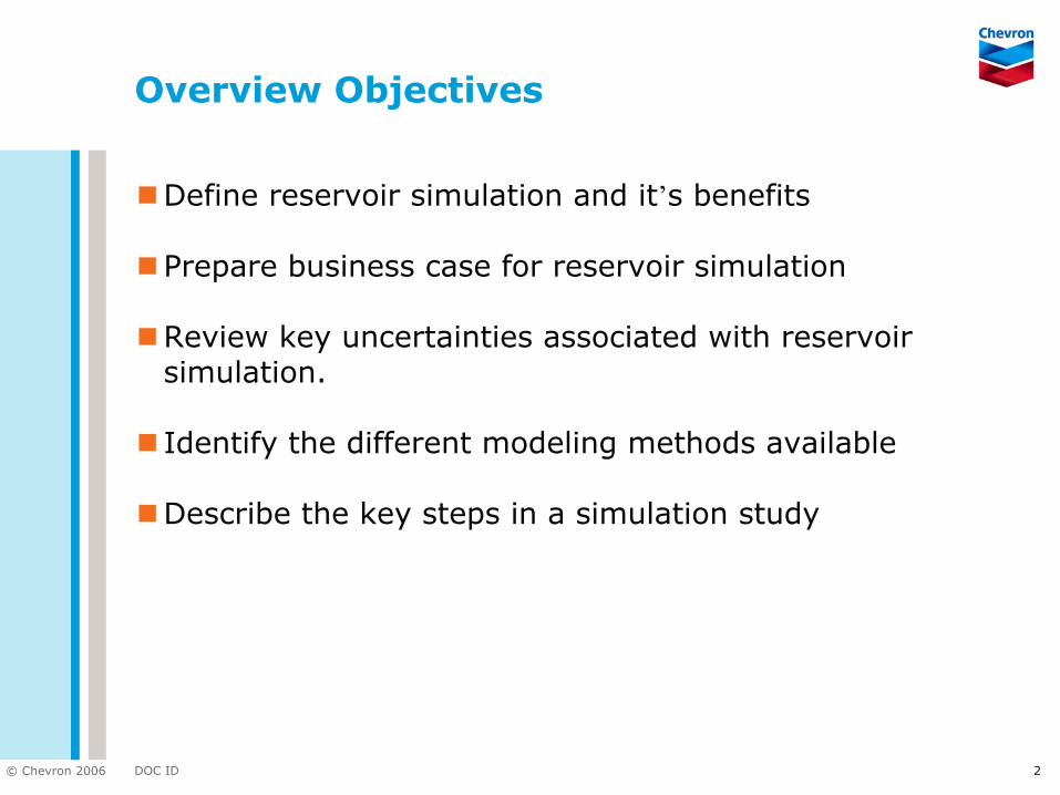
Overview Objectives

Define reservoir simulation and it’s benefits

Prepare business case for reservoir simulation

Review key uncertainties associated with reservoir simulation.

Identify the different modeling methods available

Describe the key steps in a simulation study


What is Simulation?

As applied to petroleum reservoirs, simulation can be stated as:

The process of mimicking or inferring the

behavior of fluid flow in a

petroleum reservoir system

through the use of either

physical or mathematical models


What is Simulation?

As used here, the words petroleum reservoir system include the reservoir rock and fluids, aquifer, and the surface and subsurface facilities.


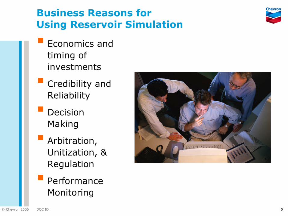
Business Reasons for Using Reservoir Simulation

Economics and timing of investments

Credibility and Reliability

Decision Making

Arbitration, Unitization, & Regulation

Performance Monitoring


Modeling Methods

Physics & Detail

Integrated Production Modeling

Finite Difference Reservoir Simulation

Streamline Simulation

Material Balance & P/Z Analysis

Decline Curve Analysis

Analogies

Com

plex

ity &

Effo

rt

• Any problem is solvable if you can make assumptions -the key is determining the right assumptions.

• Not every question demands in-depth modeling of every detail.


Modeling MethodsData Considered by Method

Well Descriptions

Location

Completion Interval

Completion Changes

Stimulations

Lab Measurements

PVT Properties

Relative Permeability

Capillary Pressure

Reservoir Description

Geometry

Petrophysical Properties

OWC’s, GOC’s

Field Measurements

Well Pressures

Oil, Water, Gas Production

Production Logs

Well Tests

Numerical Simulation

Material Balance

Decline Curve

What are the assumptions for each method?


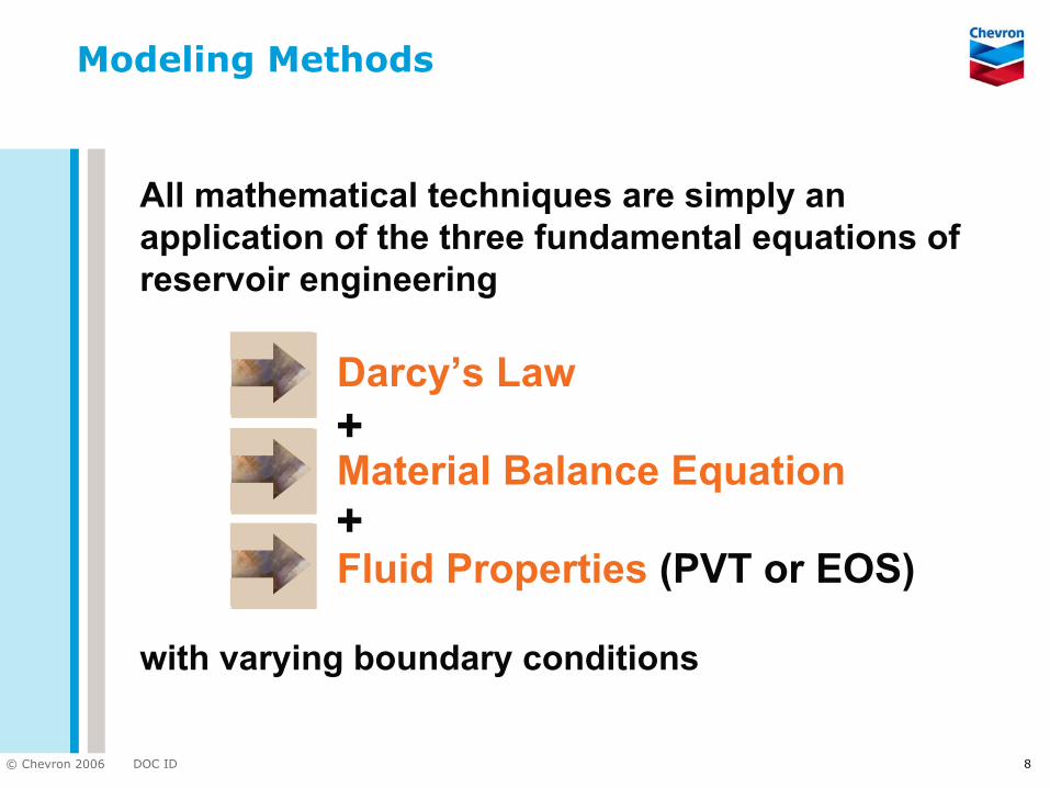
Modeling Methods

All mathematical techniques are simply an application of the three fundamental equations of reservoir engineering

Darcy’s Law

Material Balance Equation

Fluid Properties (PVT or EOS)

with varying boundary conditions

+

+


Modeling Methods

Finite Difference Process

Divide the reservoir into numerous blocks and represents it with a mesh of points or grid blocks.

Geologic Model

DetailedSimulation

Model

SimplifiedSimulation

Model

Material Balance

Model


Modeling Methods

Finite Difference 3 Step Process

Solve mathematical equations for each cell by numerical methods to obtain pressure, production and saturation changes with time.

INPUTDATA

CALCULATEDBY

SIMULATOR

FORALLTIME

ATEACHPOINT

INTIME

ONE φONE KxONE KyONE Kz

ONE PONE SoONE SwONE Sg

INPUTDATA

CALCULATEDBY

SIMULATOR

FORALLTIME

ATEACHPOINT

INTIME

ONE φONE KxONE KyONE Kz

ONE PONE SoONE SwONE Sg

The Diffusivity EquationThe Diffusivity Equation(Single Phase, 1(Single Phase, 1--D Flow)D Flow)

tPc

xP

µk

2

2

∂∂

=∂∂ φ

The Diffusivity EquationThe Diffusivity EquationThe Diffusivity Equation(Single Phase, 1(Single Phase, 1(Single Phase, 1--D Flow)D Flow)D Flow)

tPc

xP

µk

2

2

∂∂

=∂∂ φ

The Diffusivity EquationThe Diffusivity Equation(Single Phase, 1(Single Phase, 1--D Flow)D Flow)

tPc

xP

µk

2

2

∂∂

=∂∂ φ

The Diffusivity EquationThe Diffusivity EquationThe Diffusivity Equation(Single Phase, 1(Single Phase, 1(Single Phase, 1--D Flow)D Flow)D Flow)

tPc

xP

µk

2

2

∂∂

=∂∂ φ

Accuracy of data input

Impacts accuracy ofsimulator calculations


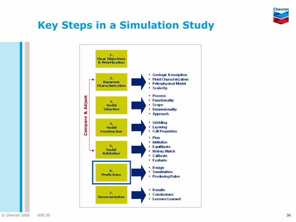
Key Steps in a Simulation Study


Pre-planning the Reservoir Simulation Study

Considerations:

Objectives of the study

Assess uncertainties

Data requirements and availability

Modeling approach

Limitations of proposed procedures

Resources

Project budget – should be related to decisions required

Time available

Hardware: PC, Workstation, , supercomputer, cluster

Software: Commercial (Eclipse®, VIP®…), in-house (such as CHEARS®)


Sources of Uncertainty in Simulation

Data Quality Data Quality & Quantity& Quantity

GeologyGeology

ScaleScale--UpUpMathematicalMathematical


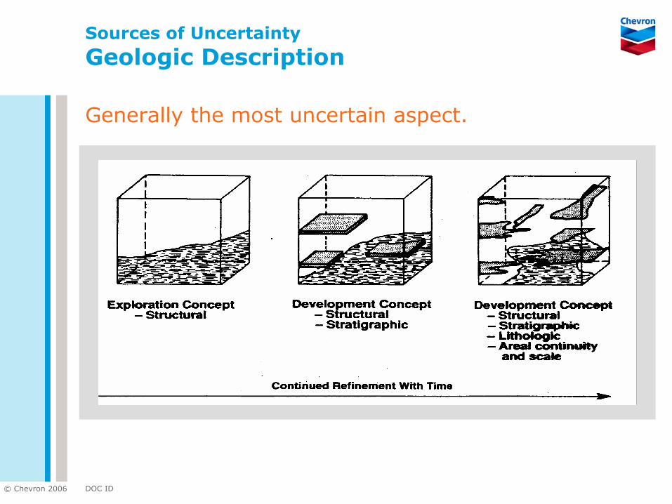
Sources of Uncertainty

Geologic Description

Generally the most uncertain aspect.


Sources of Uncertainty

Results should carry a ‘‘band of uncertainty”

Models are often asked to provide forecasts beyond the accuracy of the field data

Worsened by lack of geologic & engineering control

Model Results

Band of UncertaintyQ

Time


Step 1 – Set Clear Objectives & Priorities

Examples of Reservoir Study Goals

Typical Goals for New Fields:

Define reservoir’s internal & external boundaries

Define reservoir pay, volume, & reserves

Determine optimum number, location, & configuration of wells

Optimize timing and sizing of facilities

Select optimum recovery process

Estimate potential recovery performance

Anticipate future produced fluid & operational changes

Determine critical gas and water coning rates


Step 1 – Set Clear Objectives & Priorities

Examples of Reservoir Study Goals

Typical Goals for Mature Fields:

Monitor fluid contact movement

Evaluate productivity degradation

Evaluate historical reservoir performance. Determine why performance did not match predicted recovery

Determine source of produced water and/or gas. Identify wells with workover potential

Monitor reservoir sweep to locate by-passed oil. Specify infill drilling requirements

Estimate benefits of secondary recovery or EOR

Determine connectivity between multiple reservoirs

Quantify lease-line migration


Step 2 – Characterize the ReservoirThree Inter-Dependent Components


Step 2 – Characterize the ReservoirGeological Description

A geological description must identify the key factors which affect flow through the reservoir:


Step 2 – Characterize the Reservoir

Fluid Characterization

Fluid characterization defines the physical properties of the reservoir fluid mixture, and how they vary with changes in pressure, temperature and volume.

Steps to characterize the reservoir fluids:

• Classify the fluid type• Determine reservoir fluid

properties• Describe reservoir production

mechanisms


Step 2 – Characterize the Reservoir

Petrophysical Model

The petrophysical model defines where the volumes of oil, water and gas are located in the reservoir, as well as how fluids behave in the presence of the rock.

To define the petrophysical model of the reservoir, you must determine:

Rock Wettability

Capillary Pressure

Relative Permeability

Residual Oil Saturation

Fluid Contacts


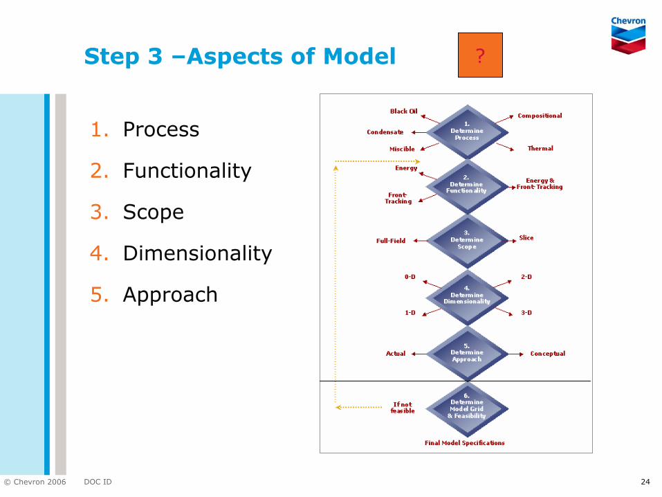
Step 3 –Aspects of Model

1. Process

2. Functionality

3. Scope

4. Dimensionality

5. Approach

?


Black Oil

Condensate

Miscible

Compositional

Thermal

Step 3 – Select the Model

Determine the Process



Determine the Functionality



Determine the Dimensionality

Use 1D models for linear or radial flow in only one direction

Use 2D models for linear or radial flow in two directions: Radial, areal, cross-sectional

Use 3D models for situations for linear or radial flow in three directions: Pattern element, segment, full-field

1-D Model

P1 P2 P3 P4

2-DRadial2-D

Radial



Determine the Approach

Detailed Geologic DescriptionMay be matched tohistoric performance

Higher Uncertainty Properties



1. Scale-up to full-field would be difficult (e.g., due to areal heterogeneities)

2. Cross-boundary fluxes are unknown and cannot be accurately estimated

Scale-up of results from a slice to full-field can be done accurately.

Must scale-up to full-field and separately estimate boundary fluxes

SimplicitySlice

Simple parameter-sensitivity studies

Scale-up of results from a slice to full-field is impractical

More complex than slice mode

Doesn’t need scale-up to full field; separate boundary fluxes unneeded

Full-Field

Energy & phase saturation distributions in time are important

More complex than energy & front tracking

Allows accurate computation of reservoir pressures & phase saturations

Energy / Front-Tracking

Large-scale field studies

Phase saturation tracking in reservoir is important

Requires very fine gridding

SimplicityFront-Tracking

Saturation distributions in time are important (i.e., infill drilling, workover planning, individual well performance)

Material balance & pressure calculation in time are important

Lacks accurate computation of phase saturation distribution

SimplicityEnergy

Unsuitability to Models

Suitability to Models

DisadvantagesAdvantagesTypeFu

nctio

nalit

yS

cope


Step 3 – Select the Model Dimensionality

Objectives necessitate validation (e.g., mature field development studies)

Reservoir data is lacking

No validation of model data

SimplicityConceptual

Reservoir and production data are sparse (i.e., virgin fields)

Allows actual characterization of reservoir

Complexity relative to conceptual

Allows actual characterization to validate model against field data

Actual

Simple parameter-sensitivity studies

3D effects are being investigated

More complex than 1D and 2D

Simulates reservoir dynamics in 3D

3D

Solutions require analysis of 3D effects (e.g., study of near wellbore effects such as coning)

2D effects are being investigated

Simulates reservoir dynamics in only two dimensions

Simplicity relative to 3D

2D

Solutions require analysis of 3D effects (e.g., study of near wellbore effects such as coning)

Dimensionality is not important

Simulates dynamics in 0/1 dimensions

Simplicity relative to 2D and 3D

0D/1D

Unsuitability to Models

Suitability to Models

DisadvantagesAdvantagesTypeD

imen

sion

ality

App

roac

h


Step 4 – Construct the Model Converting the Earth Model into a Simulation Model

1. QC the geologic model for errors and problems

2. Scale-up the model

3. Output the model in simulation format

4. Output fault information for simulation

5. Intersect reservoir wells with the model and output simulation well data

6. Output production data in simulation formats and link to wells


Step 5 – Validate the Model

Evaluate results

Develop a validation plan

Initialize the simulation model

Equilibrate the model

History match

Calibrate the model

1122

3344

5566


Step 5 – Validate the Model

Two important ideas for the proper validation of reservoir models:

History Matching must not be achieved at the expense of parameter modifications that are physically and/or geologically wrong

Even when a model is fully validated, simulation results will still have some degree of uncertainty


Step 6 – Make Predictions

Important considerations when making reservoir model predictions:

Prediction cases shouldn’t exceed capabilities of the model.

Predictions need to be consistent with field practices.

Simulation yields a non-unique solution with inherent uncertainties from:

Lack of validation (e.g., reservoirs with sparse geologic or engineering data).

Modeling or mathematical constraints because of compromises made in model selection.

Inherent uncertainties in reservoir characterization and/or scale–up to model dimensions.


Step 7 – Document the Study

Methods to document studies

Technical memorandum

Formal report

Presentation

Store data files

Share lessons learned with future project teams


Updating the Reservoir Simulation Study –Important for Large Field Studies

Data Acquisition

HistoryMatchingUpdates

PerformanceStudies

Data Acquisition

HistoryMatchingUpdates

PerformanceStudies


Petroleum Reserve Estimation, Production, and Production Sharing Contract (PSC) Short Course

Bangladesh University of Engineering and Technology

29-30 April 2008

Reservoir Simulation Examples


Dynamic Models (Main Zones Shown)

CoarseFine

Z30 M-sand map view…

Z50

Z30

Z10

Z50

Z30

Z10

3-D

Main zones contain >85% of OGIP

N

S

S

N

NS


Condensate Banking – Single Well Model

• 1690 ft radius, 1ft blocks in K direction, 45 degree blocks in J direction.

• I = 33, J = 8, K varies between 29 and 57 MD.

• 3 relative permeability regions.

• Porosity from logs, perm from core correlation.


Lower Miocene Sand DST match/Saturation Profile

reservior simulator overview

Documents