reservoir engineering aspects of horizontal...
TRANSCRIPT

Reservoir Engineering
Aspects of Horizontal Wells
PET 472 lecture notes
Spring 2012
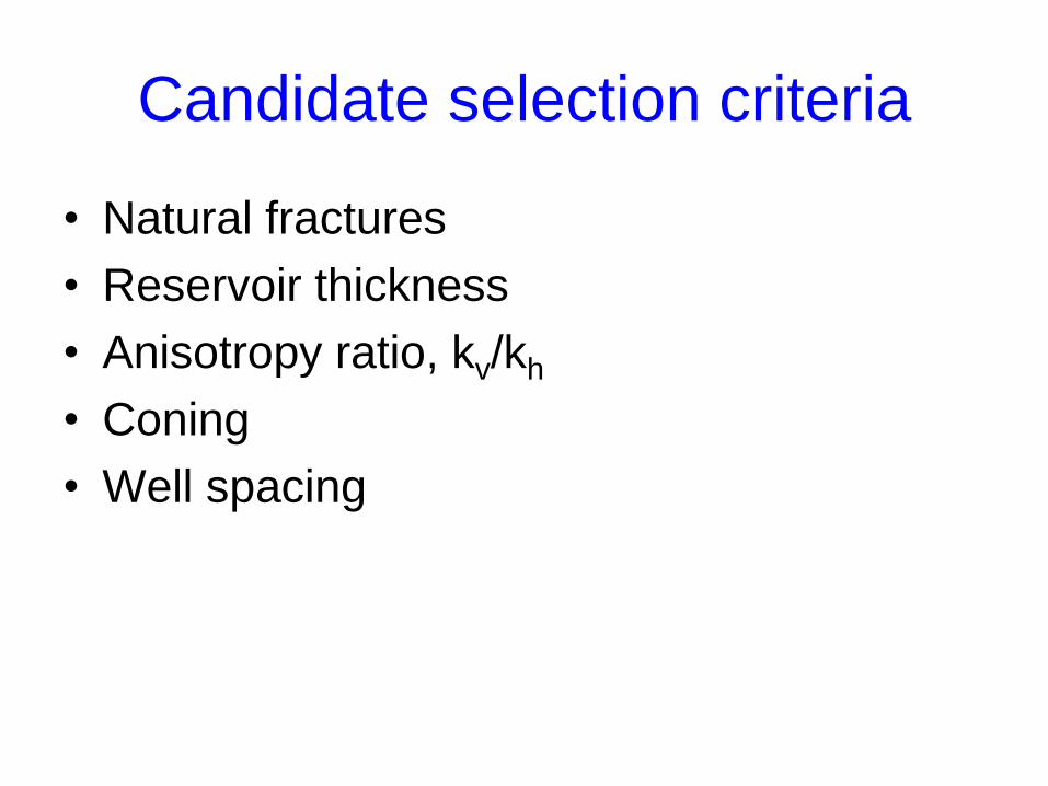
Candidate selection criteria
• Natural fractures
• Reservoir thickness
• Anisotropy ratio, kv/kh
• Coning
• Well spacing

Effect of Reservoir Thickness
vk
hk
LehrLa
L
Laa
wrhLhoBo
phhk
hq
5.04)/2(25.05.0)2/(
2/
2)2/(2
)]2/(ln[/2]ln[2.141
Steady-state solution
0
1
2
3
4
5
6
7
8
0 500 1000 1500 2000 2500
Horizontal well length,ft
Pro
du
cti
vit
y r
ati
o, J
h/J
v
h=25
h=50
h=100
h=200
h=400
Joshi

Horizontal Wells
Advantage: Horizontal well orientation to natural fracture
direction
GRM-Engler-09
kmin =
0.03 mD
kmax =
3.34 mD
kMatrix =
0.01 mDN
10 m
Horizontal well
paths
A
B
kmin =
0.03 mD
kmax =
3.34 mD
kMatrix =
0.01 mDN
10 m
kmin =
0.03 mD
kmax =
3.34 mD
kMatrix =
0.01 mDN
10 m
Horizontal well
paths
A
B

Impact of Anisotropy Ratio
0
1
2
3
4
5
6
7
8
0 500 1000 1500 2000 2500
Horizontal well length, ft
Pro
du
cti
vit
y R
ati
o, J
h/J
v
kv/kh=.1
kv/kh=.5
kv/kh=152
hk
vk
h
LDL

Drainage Area
Joshi

Drainage Area
Joshi
Drilling along the high permeability direction

Coning
Function of drawdown
Critical rate –
maximum rate only oil is produced
Joshi
Joshi

Horizontal Well Applications
1. In low permeability reservoirs, horizontal wells
enhance the drainage area for a given time period
2. In high permeability reservoirs; horizontal wells reduce
near wellbore turbulence and thus improves the well’s
deliverability
3. Single dominant pay zones, good vertical permeability
GRM-Engler-09

Horizontal Wells
• Given 400 acre lease
• 10 Vertical wells (40 ac/well)
• 6-1000-ft long horizontal
wells (74 ac/well)
• 4-2000-ft long horizontal
wells (108 ac/well)
GRM-Engler-09
Joshi, 1991
Advantage: Well spacing and location

Horizontal well
• Single phase (liquid) flow
• Pseudosteady state…bounded reservoir
• Horizontal well is located arbitrarily within the bounded drainage
area
• Horizontal well is assumed to have infinite conductivity
Constraints

Wellbore pressure drop
Uniform wellbore pressure
(Infinite-conductivity model)
Uniform flux entry
Observed triangular
profiles

Pseudosteady state equations
skin mechanicalmS
fracturety conductivi-infinite
gpenetratin-fully toduefactor skin ),4/ln(fS
factorskin related shape
386.175./ln2.141
/
wrL
CAS
where
mSfSCASwrer
oBohk
hJ
1. Based on infinite-conductivity horizontal well
Mutalik,etal

Pseudosteady state equations
e2xL when 0rS plane, areal
in then penetratio partial toduefactor skin rS
plane verticalin the area drainage h,e2y A
factor shape
)ln(75./ln2.141
/)2(
hC
where
rShCwrA
oBovkykex
hJ
2. Based on uniform flux horizontal well
Babu & Odeh

Pseudosteady state equations
direction zin factor pseudoskinzS
geometry offunction
/)/2(2.141
/2
F
where
zSvkhkLhF
oBohhk
hJ
3. Based on pressure averaging along the horizontal length
Kuchuk et al
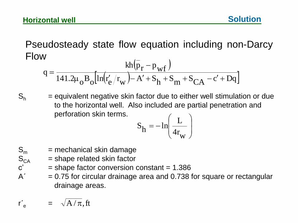
Pseudosteady state flow equation including non-Darcy
Flow
DqcCASmShSAwrerlnoBo2.141
wfprpkhq
Sh = equivalent negative skin factor due to either well stimulation or due
to the horizontal well. Also included are partial penetration and
perforation skin terms.
Sm = mechanical skin damage
SCA = shape related skin factor
c’ = shape factor conversion constant = 1.386
A´ = 0.75 for circular drainage area and 0.738 for square or rectangular
drainage areas.
r´e =
Horizontal well Solution
ft,/A
wr4
LlnhS

SCA - horizontal well shape-related skin factor
hk
vk
h2
LDL
Joshi,1991
Horizontal well Solution
For square drainage area
L/2xe

A horizontal well drilled in an oil reservoir has the following parameters.
Area = 160 acres rw = 0.365 ft
h = 50 ft kv/kh = 0.1
o = 0.5 cp kh = 1 md
Bo = 1.2 rb/stb Sm = 0
D = 0
Calculate the pss productivity index of a 2000-ft long horizontal well.
Step 1:
Horizontal well Example
ft1489/)43560)(160(/Aer
Step 2:
22.7)365.0(4
2000ln
wr4
LlnhS

SCA - horizontal well shape-related skin factor
32.6
1.0)50(2
2000
hk
vk
h2
LDL
Joshi,1991
Horizontal well Solution
For square drainage area
L/2xe=2000/2640
= 0.757
Step 3:
SCA = 2

Pseudosteady state flow equation,
psi/stb61.0
0386.10.2022.7738.0365.01489ln)2.1)(5.0(2.141
)50(1
p
q
Horizontal well Example
Jh, stbd/psi, Horizontal well productivity
kv/kh = 0.1 kv/kh = 0.5 kv/kh = 1.0
0.61 0.75 0.80

Horizontal Well Performance
• PIhorizontal > xPIvertical
• If less than expected, possible cause is
Lproductive < Ldrilled.
– Reservoir heterogeneity
– Wellbore pressure drop
– Formation damage

Estimate the fluid invasion and damage in heterogeneous
reservoirs
A heterogeneous reservoir is generated (zone A to E)
Permeability, porosity, and relative permeability curves are different in each zone
Invasion at 11 nodes from heel to toe are simulated
0 1 2 3 4 5 6 7 8 9 1
0
Reservoir type
A B C D E
k = 300 md 80 md 10 md 200 md 70 md
= 0.23 0.12 0.09 0.22 0.15
Kro, max = 0.75 0.7 0.6 0.75 0.7
no = 1.5 2 3 1.5 2
Supalak’s dissertation

Skin factors => 4.6 – 19.6 along the well
Zones B and C have severe damage
Zones D and E have the least damage
0
20
40
60
80
012345678910
Node no.
Da
ma
ge
ra
diu
s, in
.
0
10
20
30
40
50S
kin
fa
cto
r
rs, in.
s node
Skin damage and damage radius in a
horizontal well with a heterogeneous reservoir
A B
C
D E
Reservoir heterogeneity
Supalak’s dissertation

Formation damage in horizontal wells
• Larger contact area
• Longer contact time
Is the damage more vulnerable
in horizontal wells?
Fig. 2: Fluid filtration in vertical and horizontal wells
Reservoir
rock !!!
Supalak’s dissertation

L
Le av, max
aH, max
Heel
Formation damage in horizontal wells
Supalak’s dissertation

Horizontal Wells
Pseudosteady state flow equation including non-Darcy
Flow
GRM-Engler-09
DqcCASmSS75.wrerlnizT1422
2wf
p2rpkh
q
S = equivalent negative skin factor due to either well stimulation or due to the
horizontal well. Also included are partial penetration and perforation skin
terms.
Sm = mechanical skin damage
SCA = shape related skin factor
c’ = shape factor conversion constant

Horizontal Well Example
GRM-Engler-09
An oil company recently signed an offshore reservoir concession. The lease
concession lasts only for a period of 5 years. The gas is to be delivered to a
pipeline operated at 300 psia. To meet this high-pressure requirement, it is
important to maintain a wellhead pressure of 500 psia. Before testing, the test
well, which is vertical, was cemented, perforated and cleaned using acid. The
perforated interval in the vertical well was 60 ft. The reservoir has a bottom
water zone separated by a 10-ft thick layer of shale (kv/kh = ?). It appears the
reservoir is not in communication with the bottom water.
An engineer suggests drilling a 2000-ft horizontal well not only to reduce near-
wellbore turbulence but also to ensure against water coning. Compare the IPR
curves for a vertical and horizontal well in this reservoir.

Horizontal Well Example
GRM-Engler-09
60’ =14%, k =6 md, kv/kh=.1
Tr=185°F, Pr = 3400 psi, g = 0.605
7870’
5.5” ID
Ppipeline = 300 psi Pwh = 500 psi
Twh=75°F
Sw=30%
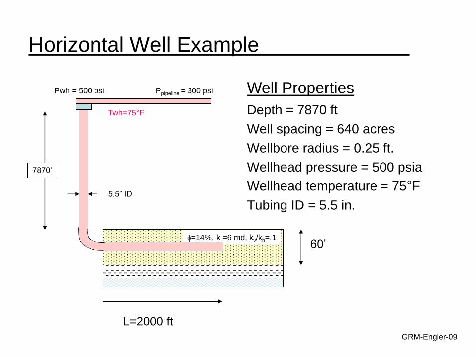
Horizontal Well Example
Depth = 7870 ft
Well spacing = 640 acres
Wellbore radius = 0.25 ft.
Wellhead pressure = 500 psia
Wellhead temperature = 75°F
Tubing ID = 5.5 in.
GRM-Engler-09
Well Properties
60’ =14%, k =6 md, kv/kh=.1
7870’
5.5” ID
Ppipeline = 300 psi Pwh = 500 psi
Twh=75°F
L=2000 ft

Horizontal Well Example
Vertical Well Performance
GRM-Engler-09
S = 0, fully penetrating vertical well
Sm = 0, no mechanical skin damage, well was cleaned with acid
SCA = 0, well centrally located in the drainage area
c’ = 0, shape factor conversion constant for vertical well.
pwf2phwr
kh1510x222.2D
g
201.1k
1010x33.2
Laminar Steady state components
Non-Darcy components
where
aC
62.31ln
caS

Horizontal Well Example
Horizontal Well Performance
GRM-Engler-09
Laminar Steady state components
Non-Darcy components
S = -7.6, negative skin due to horizontal well
Rwa = L/4 = 2000/4 = 500 ft
6.725.0
500ln
rw
warlnS
Sm = 0, no mechanical skin damage, well was cleaned with acid
c’ = 1.386, shape factor conversion constant for horizontal well.
Replace hp with L
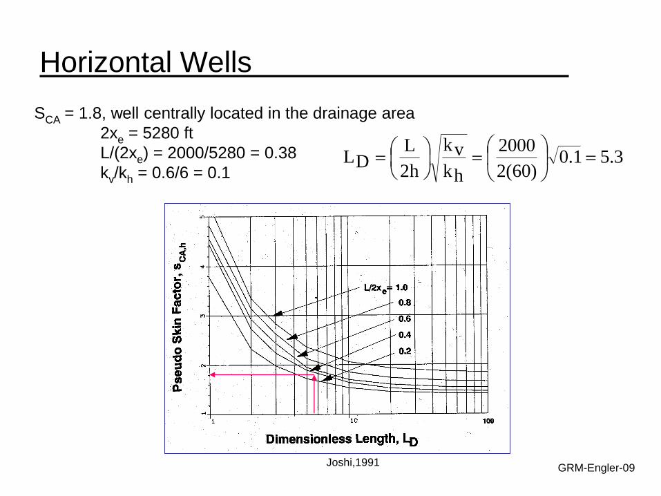
Horizontal Wells
GRM-Engler-09
SCA = 1.8, well centrally located in the drainage area
2xe = 5280 ft
L/(2xe) = 2000/5280 = 0.38
kv/kh = 0.6/6 = 0.1 3.51.0
)60(2
2000
hk
vk
h2
LDL
Joshi,1991

Horizontal Well Example
GRM-Engler-09
0
500
1000
1500
2000
2500
3000
3500
4000
0 50 100 150 200 250
gas rate, mmscfd
pre
ssu
re,
psi
B&B
C&S
IPR-horizontal
IPR-vertical
w/turbulence w/turbulence