reservoir simulator practical -...

Reservoir Simulator Practical

Course Notes 2011

Philipp Lang IZR Room 403

Tel 3004

[email protected]

for further information please refer to the accompanying document ‘Info Sheet & Course

Logistics’

mailto:[email protected]

Module I: Single Phase Flow

The term ‘single phase’ in reservoir engineering refers to systems which contain water, oil or

gas only. To be more specific, we consider single phase systems as porous media saturated

exclusively with water (i.e. as the only ‘phase’). Flow in such a porous medium, or any domain

for that matter, occurs due to a difference in potential (i.e. pressure). We will look into how such

pressure gradients (differences) arise within reservoir systems, their impact on flow response and

dependence on material/upscaled properties. For complex systems numerical methods and partial

differential equations will be presented that allow us to emulate and predict dynamic behavior of

reservoirs. Further, we will use the gained information to upscale flow properties ourselves that

accurately describe reservoir behavior on different scales.

NB: These lecture notes are supposed to be read ‘in one piece’ as it also serves as a walk through for the

lab exercises. The material presented will help you understand the concepts covered in class. It does not

serve as a substitute for attending the course (considered as auxiliary only).

Pressure and Flow ...................................................................................................................................... 1

Steady State Pressure ............................................................................................................................. 1

Flow Response ........................................................................................................................................ 2

Real World Complexity – Need for Discretization ............................................................................ 3

A Diffusion Equation ............................................................................................................................. 6

Transient Pressure ................................................................................................................................ 10

Assumptions ......................................................................................................................................... 11

Flow Properties ......................................................................................................................................... 12

Scales and the REV ............................................................................................................................... 12

Effective Permeability: Hands-on upscaling .................................................................................... 13

Related BSc Examination Concepts ....................................................................................................... 18

References .................................................................................................................................................. 19

RSP Module I: Single Phase Flow 1

Pressure and Flow

This section will introduce into how complex systems are divided (discretized) into smaller,

simpler systems to allow numerical solutions of problems described by PDEs (partial differential

equations). Specifically, the steady state solution of pressure (computing pressure at various

points within a domain) is discussed, and its corresponding flow response. This part of the

lecture notes deals exclusively with single phase systems.

Steady State Pressure

We use the term ‘steady state’ to describe the fact that pressure (our potential responsible for

fluid flow) does not change over a given period of time. This implies that a constant pressure

field (a scalar field that is) can be observed in the domain of interest (our reservoir).

A basic constitutive relationship (a relationship that describes the mutual dependence of two

physical variables) that relates fluid flow and pressure is attributed to Darcy (1856), we recall:

(1)

To be more specific, (1) relates flow rate (q, in meters per second) to a pressure gradient (in

Pascal per m). In plain terms we can say that for a high pressure difference flow will be high.

Also, the relation between pressure drop and flow velocity is directly proportional to the

permeability-viscosity ratio, which in reservoir engineering is widely referred to as conductivity.

This takes into account the absolute permeability (since we are dealing with single phase flow) of

the rock and the viscosity of the fluid, hence providing a measure of resistance to flow/pressure.

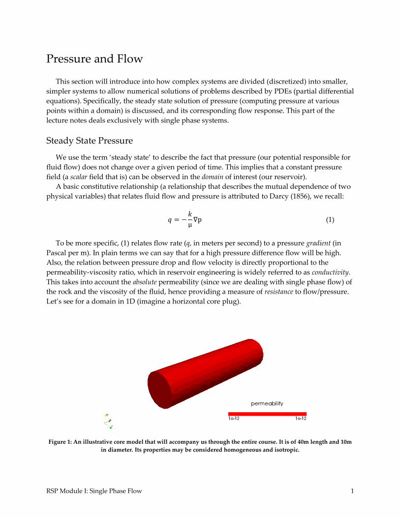
Let’s see for a domain in 1D (imagine a horizontal core plug).

Figure 1: An illustrative core model that will accompany us through the entire course. It is of 40m length and 10m

in diameter. Its properties may be considered homogeneous and isotropic.


We apply a pressure of 2.0x105 Pa at the bottom right end and keep pressure at the upper left

end at atmospheric level (1.0x105 Pa). Further we consider the hull impermeable, or sealed for

that matter (i.e. no flow through it). Under the assumption of a steady state regime, the pressure

distribution (the value of pressure at different points along the x-axis for our plug) looks as such:

Figure 2: Steady state pressure distribution in our core model. A pressure difference of 1 bar was applied, resulting

in a gradient of 0.025 bar/m. The plot on the right shows pressure in Pa on the

This linear distribution (a line with constant gradient) reflects the relationship of direct

proportionality between pressure gradient and permeability-viscosity ratio in (1), Δp and k/μ

respectively. For a homogeneous and isotropic domain of such geometrical simplicity this

solution appears trivial to come by, and indeed it is (i.e. analytically).

Figure 3: Visualizing pressure using evenly distributed contours (i.e. each disc represents points of equal pressure,

with a fixed interval between each disc)

Flow Response

For the pressure profile presented in Figure 2 and Figure 3, we are now going to look at the

response of fluid flow within our core. As with current in electrical systems, flow is

perpendicular to lines of equal potential (i.e. our pressure contours). This is illustrated by a

sketch in Figure 4:


Figure 4: Illustrating flow vectors perpendicular to equipotentials (pressure contours). The images in the

background of your local weather man will pretty much look alike.

This is just one example of how different phenomena in nature relate to each other, which is

obvious when comparing fundamental relationships as derived by Ohm, Fourier and Darcy.

Back at our core model, velocity is uniform across our sample, since the pressure gradient is

uniform (or constant) and (1). We arrive at the velocity by using (1) and assuming a permeability

of 1.0x10-12 m2 (or roughly one Darcy) and a viscosity of 5.0x10-4 Pa.s(or 0.5 centipoise).

Figure 5: Velocity vectors visualized along pressure contours (equipotential). Their magnitude is around 5.0x10-6

meters per second (‘Darcy’ or apparent velocity) for a permeability of 1 Darcy and fluid viscosity of 0.5 centipoise

under the established pressure gradient.

In order to arrive at a volume flux (the volume of fluid flowing through the porous medium

per time that is), the Darcy flow velocity as established above is simply to be integrated over

(here: multiplied by) the cross sectional area of interest. For our core example that yields about

100 ml per second or 111 liters per day (give or take).

Real World Complexity – Need for Discretization

Our desire to understand and predict dynamic behavior of large and structurally complex

domains renders analytical solutions for phenomena of the likes of pressure, flow/transport and

many more (of thermal, chemical and mechanical nature) unfeasible. Imagine our core (which is

pretty huge after all), now with distinct heterogeneities (highly permeable ‘bubbles’):


Figure 6: Introducing highly permeable heterogeneities (artificial bubbles) to our core plug. Permeability contrasts

by a factor of 10.

An analytic or intuitive solution for the pressure distribution, and hence velocity field, seems

hard to come by, and indeed it is. This is where numerical methods and partial differential

equations come into play and provide us with an approximated solution as such:

Figure 7: Numerical solution of pressure for a heterogeneous domain. Pressure contours are not of plain disc shape

anymore but honor the high permeability structures. NB: The pressure interval between contours is less than in

the previous figures.

A closer look at the vicinity of the highly permeable bubbles reveal the nature of pressure

distribution as a result of the contrast in conductivity (remember single phase conductivity

being the ratio of permeability and viscosity and, since the latter remains unchanged, higher

permeability results in higher conductivity, i.e. less resistance to pressure propagation).


Figure 8: A closer look at the pressure response (pressure distribution due to imposed pressures at the domain

boundaries). Pressure contours evolve around features of high permeability, since the pressure drop within them

is much less as compared to the less conductive surrounding.

Before we go further into discussing the resulting fluid flow behavior for our ‘evolved’ core,

we take a step back. We agreed upon the fact that for structurally complex systems striving for

an analytic solution is pointless. So how do we actually simulate the behavior of such systems?

The approaches of choice may be summarized by the term numerical methods. Since the focus

of this course is on practical aspects much rather than theoretical considerations, this will be a

very brief introduction to numerical methods used in reservoir simulation.

The entire concept revolves around discretizing a domain of interest. This describes the

process of ‘dividing’ a continuous domain into a finite number of discrete parts while keeping a

proper representation. Figure 9 illustrates for our core model:

Figure 9: Discretizing our core in space (transforming from continuous to discrete)


The right hand side of Figure 9 shows a so called mesh. It consists of a finite number of so

called elements, or cells. There is a number of different kinds of meshes, or discretization (in

space), but we won’t go into detail here. The basic idea is to form our domain out of an

arrangement of grid blocks (yet another synonym) for which properties are constant. That

means for each cell, there is only one value for porosity, permeability and others.

Figure 10: A box model discretized in a regular manner, consisting of 1600 grid blocks. Each grid block is of

constant permeability.

Depending on the type of the element and its dimensions, we can come up with an equation

that describes its behavior. We then go on and assemble a system of equations that we use to

describe the behavior of the domain as a whole. So we break down a complex structure into

basic geometrical units (which we can solve for) and compute their interaction numerically.

A Diffusion Equation

Upon discretizing our domain in space, numerical methods such as the finite element

approach allow us to solve differential equations that describe the behavior of the system of

interest. A popular starting point for deriving such equations is pretty simple:

(2)

But what does this mean? No change in volume flow. (2) states that the change ( , the

divergence) of volume flowing (u, i.e. m3 per second) is zero. If the flow does not change (that’s

what (2) is all about), everything entering a certain volume (Figure 11) has to be compensated by

something leaving that volume. I admit that doesn’t sound too exciting, but we just stated a

conservation law that allows us to build upon.


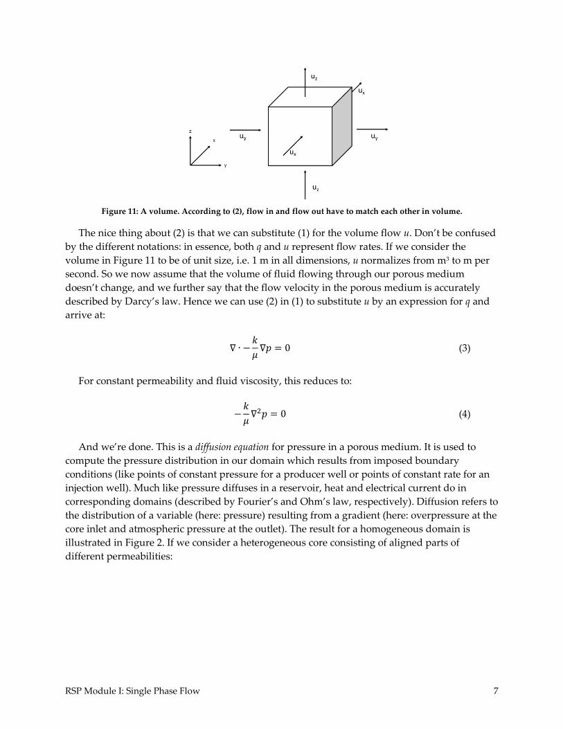
Figure 11: A volume. According to (2), flow in and flow out have to match each other in volume.

The nice thing about (2) is that we can substitute (1) for the volume flow u. Don’t be confused

by the different notations: in essence, both q and u represent flow rates. If we consider the

volume in Figure 11 to be of unit size, i.e. 1 m in all dimensions, u normalizes from m3 to m per

second. So we now assume that the volume of fluid flowing through our porous medium

doesn’t change, and we further say that the flow velocity in the porous medium is accurately

described by Darcy’s law. Hence we can use (2) in (1) to substitute u by an expression for q and

arrive at:

(3)

For constant permeability and fluid viscosity, this reduces to:

(4)

And we’re done. This is a diffusion equation for pressure in a porous medium. It is used to

compute the pressure distribution in our domain which results from imposed boundary

conditions (like points of constant pressure for a producer well or points of constant rate for an

injection well). Much like pressure diffuses in a reservoir, heat and electrical current do in

corresponding domains (described by Fourier’s and Ohm’s law, respectively). Diffusion refers to

the distribution of a variable (here: pressure) resulting from a gradient (here: overpressure at the

core inlet and atmospheric pressure at the outlet). The result for a homogeneous domain is

illustrated in Figure 2. If we consider a heterogeneous core consisting of aligned parts of

different permeabilities:


Figure 12: Core with sections of different permeabilities.

The pressure distribution resulting from the very same boundary pressures as computed by

solving our diffusion equation (4) looks as such (compare to Figure 2):

Figure 13: Steady state pressure distribution for a heterogeneous core of sections with different permeabilities.

Note the straight line solutions for each section of uniform permeability with different gradients.

Up to now, the diffusion equation (4) allows us to compute the pressure distribution within a

porous media domain resulting from fixed points of pressure (here: core inlet and outlet). But

pressure is of course influenced by injection/production as well. In reservoir simulation terms

we refer to sources/sinks (for fluid injection and withdrawal, respectively). Conveniently,

accounting for volume sources in (4) is relatively straight forward: all we need to do is add a

source/sink term q:

(5)

The source term q is zero at every point in our domain where no inflow/outflow occurs,

hence reducing to (4). We can use this extended diffusion equation to compute the pressure


distribution for our homogeneous core for the case of a source (i.e. we ‘add’ fluid volume) in the

center of the core:

Figure 14: Steady state pressure distribution for a homogeneous core with a fluid source in the center. Look at the

increase in pressure at the point of the source. The pressure at the inlet and outlet remain fixed as in the previous

cases.

Now we’re somewhat ready to go back to the flow that developed in our high permeability

bubbles core as a response to the potential field (our pressure gradients). Since flow is

perpendicular to surfaces of equal pressure, and pressure contours are not plain discs anymore

(due to heterogeneities), flow paths change accordingly. That means flow is not perpendicular to

the core boundary as illustrated in Figure 4 and Figure 5, but very much deviated. Figure 15

illustrates.

Figure 15: Flow as illustrated by streamlines and vectors in response to the steady state pressure distribution for

out modified core. We see a focusing in the high permeable regions, as flow is redirected towards those regions

(for the pressure gradient wraps around these regions) and also is highest in magnitude (flow speed, mass flow).


In class we will address in more detail the pressure distribution and flow response for the

scenario above, as well as for the case when the bubbles become less permeable than the

surrounding matrix. Developing an intuitive understanding for how conductivity contrasts

influence pressure and flow is an essential asset that applies to various kinds of subsurface

structures (faults, fractures and all kinds of diagenetic and sedimentary heterogeneities).

Transient Pressure

The steady state solutions presented up to here imply that any change in pressure (also

caused by sources/sinks) at any point is ‘felt’ immediately in the entire domain, i.e. pressure

propagates with infinite speed. For a number of reasons (fluid and rock compressibility), this is

of course not an accurate description. It takes time for pressure changes to propagate through

the porous medium, so that once we put a well on production for example, the pressure at most

points in the reservoir remains unchanged for an extended period of time. Let’s go back to our

core to illustrate the effect. We assume our core is initially under atmospheric pressure, so

1.0x105 Pa at any point.

Figure 16: Initial state of pressure distribution in our core. Pressure is constant atmospheric.

This initial state is defined by us to provide the simulation software with a starting point,

widely referred to as initial conditions. The need for providing this initial state arises from the fact

that now we deal with pressure distribution that changes with time, as opposed to the steady state

solution that remains constant over time. So in essence we need to specify to any simulation

software the starting point for transient problems (we predict the change of our reservoir over

time after all). Once this starting point (the virgin state of our reservoir) is defined, we impose

boundary conditions. These are known (by us, the engineers) conditions at certain point in the

domain, for example aquifer contact and well rates or pressures. In our case we impose pressure

at the inlet and outlet of the core. Computing the pressure yields now different distributions for

advancing time steps:


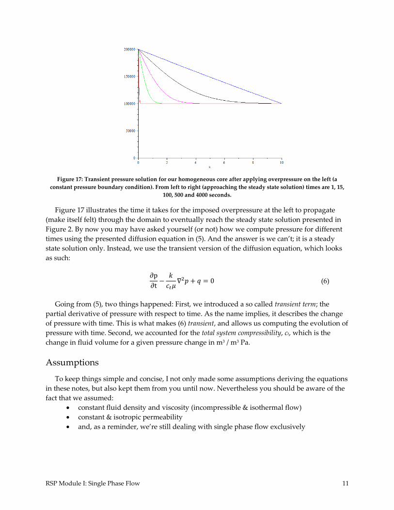
Figure 17: Transient pressure solution for our homogeneous core after applying overpressure on the left (a

constant pressure boundary condition). From left to right (approaching the steady state solution) times are 1, 15,

100, 500 and 4000 seconds.

Figure 17 illustrates the time it takes for the imposed overpressure at the left to propagate

(make itself felt) through the domain to eventually reach the steady state solution presented in

Figure 2. By now you may have asked yourself (or not) how we compute pressure for different

times using the presented diffusion equation in (5). And the answer is we can’t; it is a steady

state solution only. Instead, we use the transient version of the diffusion equation, which looks

as such:

(6)

Going from (5), two things happened: First, we introduced a so called transient term; the

partial derivative of pressure with respect to time. As the name implies, it describes the change

of pressure with time. This is what makes (6) transient, and allows us computing the evolution of

pressure with time. Second, we accounted for the total system compressibility, ct, which is the

change in fluid volume for a given pressure change in m3 / m3 Pa.

Assumptions

To keep things simple and concise, I not only made some assumptions deriving the equations

in these notes, but also kept them from you until now. Nevertheless you should be aware of the

fact that we assumed:

constant fluid density and viscosity (incompressible & isothermal flow)

constant & isotropic permeability

and, as a reminder, we’re still dealing with single phase flow exclusively


Flow Properties

Constitutive relationships in reservoir engineering make extensive use of material and fluid

properties, such as permeability, porosity and viscosity, just to name a few. Some properties,

however, may differ in value depending on the scale they were obtained (computed, measured)

from. As an example, we measure permeability at the core scale (i.e. 20x50 cm) and apply it to

elements/grid blocks which are of 100 meters in each direction (upscaling), and expect to

accurately predict behavior. We will briefly look into the basic concepts of upscaling and then

proceed with an illustrative example.

Scales and the REV

The concept of the representative elementary volume (REV) arises from the fact that it is not

feasible to measure properties at any arbitrary point in our reservoir. In fact, we measure the

likes of porosity, permeability and many more only at a few locations that are of negligible size

when compared to the reservoir as a whole. We then go on and suggest that these values,

measured from e.g. a 20 x 50 cm core, are representative for parts of our reservoir which are e.g.

200x500 m in size. This is what upscaling is all about, where we try to figure out the property

distribution for the entire reservoir, discretized in presumably large grid blocks, from few

measurements of very small samples. Heinemann (2004) illustrates the relation between a

property (here: Φ), a scale and the corresponding values obtained through measurements:

Figure 18: For porosity, a characteristic scale may exist for which measured values are representative (Heinemann,

2004)

This shows that there is a limited scale for most properties where they can be measured at

and applied for (in a meaningful way). This becomes very important with regards to the

discretization concept introduced in these notes. If porosity is measured on the core or short to

medium range well log scale, applying the acquired value to grid blocks of a couple of 100

meters in diameter raises crucial questions. Is the measured value still representative? Will the

yielded simulation results predict the behavior accurately?


Figure 19: Illustrating the concept of REV; a sample that is representative for different scales; usually based on a

property which obeys a distribution a meaningful mean can be established for.

Effective Permeability: Hands-on upscaling

Let’s start by looking at a homogeneous and isotropic cube, which could represent a part of a

reservoir domain. We apply the by now well-known constant pressure boundary conditions on

the left and right side along the x-axis and compute for pressure and flow. The result is

illustrated in Figure 20.

Figure 20: Pressure solution and flow response for a homogeneous cube, using constant pressure boundary

conditions to apply a gradient from left to right along the x-axis.

The solution looks pretty straight forward and is in agreement with our core flood shown in

Figure 5. If we were now to apply the same set of boundary conditions (opposing high and low

pressure) along different axes (i.e. the y- and z-axis), we would get the same solution (pressure

distribution and flow velocity) for the corresponding orientation, shown in Figure 21:


Figure 21: Pressure and velocity for boundary conditions along the y (left) and x (right) axis.

This illustrates the isotropic characteristic of the cube with respect to permeability. For an

anisotropic porous medium, permeability may be described by a tensor as such:

{

} (7)

For a principle coordinate system this reduces to:

{

} (8)

Visualizing this permeability tensor for our isotropic cube as an ellipse would look like:

Figure 22: The isotropic permeability tensor visualized as an ellipse is of spherical shape.

Since the tensor reduces to the effective permeability in all orientations:

{

} (9)


Which implies equal resistance to flow no matter the orientation of the pressure gradient.

Let’s now assume a single highly permeable fracture within the center of our cube:

Figure 23: A highly permeable fracture (factor 10) in the center of the cube. It is of elliptical plain shape and

oriented along the y-axis.

We will look into two questions that arise now: How will this fracture affect the pressure and

flow in our domain? How will it do so for different orientations of the boundary conditions (as

in Figure 21)? Since the fracture has a preferential orientation and is of contrasting permeability,

it will have different influence on the overall (upscaled) permeability of the cube depending on

the orientation of the pressure gradient. We start out by applying a differential along the x-axis:

Figure 24: Flow along the x-axis> Pressure contours evolve around the high permeable zone (left), and flow

(streamlines, right) focus on it.

We see that the fracture contributes to the overall (ensemble) permeability of our cube by

providing a zone of less resistance. This gets more severe if we look at flow along the y-axis,

since this is the preferential orientation of the fracture (the axis along which the fracture is

largest in size):


Figure 25: Pressure differential along the preferential orientation of the fracture (y-axis). Pressure contours are

more bend and flow shows higher focus (stream lines) than in Figure 24.

So for this orientation of the pressure gradient our fracture contributes the most to the total

permeability of the block (it assists the most in providing its maximum length as flow path). For

a gradient along the z-axis however, no contribution from the fracture to permeability may be

observed due to its perpendicular orientation. It does not provide for a flow path:

Figure 26: For flow along the z-axis, no contribution of the fracture is provided in terms of flow, since its

orientation is parallel to pressure contours (equipotentials). Flow is uniform over the entire cube.

The findings of our flow experiments along different orientations for a cube containing a

heterogeneity may be expressed in terms of an upscaled permeability tensor. We saw that the

highest permeability (highest contribution of the fracture) occurs along the y-axis. Less

contribution is provided to flow along the x-axis and no contribution to flow along the z-axis.

We illustrate this in terms of increase in permeability as a factor of the matrix permeability km:


{

} (10)

These values can be obtained by evaluating the results of our numerical simulation. To be

more specific, we use (1) to derive the total permeability along each axis by inserting q (the total

flow across the cube, illustrated by the velocity vectors), the imposed Δp and the fluid viscosity.

We can use this computed permeability to predict the behavior of a grid block without explicitly

modeling the fracture, and still obtain similar results. This is an example of upscaling. To

illustrate the above (anisotropic) permeability tensor:

Figure 27: An anisotropic permeability tensor with the largest component along the y-axis (kyy), and the minimum

along the z-axis (kzz)


Related BSc Examination Concepts

- Homogeneous versus heterogeneous porous media

- REV

- Darcy’s law

- Darcy (average) velocity vs. interstitital velocity

- Conservation laws (mass, momentum, energy)

- Pressure diffusion equation (steady-state and transient)

- Hydraulic diffusivity

- Storativity / total system compressibility

- Visualization using contours, shading, vectors and streamlines,

- Partial differential notation (divergence, gradient, curl Laplacian etc.)


References

J. Bear (1972). Dynamics of Fluids in Porous Media. Dover Publications, Inc, New York.

O. M. Phillips (1991). Flow and Reactions in Permeable Rock. Cambridge University Press,

ISBN 0-521-38098-7.

F. A. L. Dullien (1992). Porous Media: Fluid Transport and Pore Structure. 2nd ed.,

Academic Press, ISBN 0-12-223651-3 (1992).

Heinemann (2005). Textbook Series. Fluid Flow in Porous Media. Vol. 1, Leoben

Chen, Zhangxing (2007). Reservoir Simulation – Mathemetical Techinques in Oil Recovery.

Society for Industrial and Applied Mathematics ISBN 978-0-898716-40-5

Fanchi, J.R. (2006). Principles of Applied Reservoir Simulation (3rd Edition). Gulf Professional

Publishing (Elsevier), Oxford ISBN 987-0-7506-7933-6

Lake, L.W. (1989). Enhanced Oil Recovery. Prentice Hall, New Jersey ISBN 0-13-281601-6

Montaron, B., Bradley, D., Cooke, A., Prouvost, L., Raffn, A., Vidal, A., & Wilt, M. (2007). Shapes

of Flood Fronts in Heterogeneous Reservoirs and Oil Recovery Strategies. Proceedings of

SPE/EAGE Reservoir Characterization and Simulation Conference. Society of Petroleum

Engineers. doi:10.2523/111147-MS

Fanchi, J. R., Christiansen, R. L., & Heymans, M. J. (2002). Estimating Oil Reserves of Fields With

Oil/Water Transition Zones. SPE Reservoir Evaluation & Engineering, 5(4), 3-5.

doi:10.2118/79210-PA

Sohrabi, M., Henderson, G., Tehrani, D., & Danesh, A. (2000). Visualisation of Oil Recovery by

Water Alternating Gas (WAG) Injection Using High Pressure Micromodels-Water-Wet System.

SPE Annual Technical Conference and Exhibition.

Youssef, S., Bauer, D., Bekri, S., Rosenberg, E., & Vizika-kavvadias, O. (2010). 3D In-Situ Fluid

Distribution Imaging at the Pore Scale as a New Tool For Multiphase Flow Studies. SPE Annual

Technical Conference and Exhibition.

reservoir simulator practical -...

Documents