resferences and design aids for envrionmental … aids_vol_ii_nwd.pdfhandbook – hydrology,...
TRANSCRIPT
REFERENCES AND DESIGN AIDS
FOR ENVIRONMENTAL RESOURCE PERMIT
APPLICANT’S HANDBOOK VOLUME II
FOR USE WITHIN THE GEOGRAPHIC LIMITS OF
THE NORTHWEST FLORIDA WATER MANAGEMENT DISTRICT
Applicant’s Handbook, Volume II (including all Appendices) is incorporated by reference in Rule 62-330.010, F.A.C.
These References and Design Aids are not incorporated by reference in Chapter 62-330, F.A.C., and therefore do not constitute rules of the Agencies. They are
intended solely to provide applicants with useful tools, example calculations, and design suggestions that may assist in the design of a project
FLORIDA DEPARTMENT OF ENVIRONMENTAL PROTECTION
AND NORTHWEST FLORIDA WATER MANAGEMENT DISTRICT
August 16, 2013
DEP-NWFWMD ERP References and Design Aids August 16, 2013 DA - i
TABLE OF CONTENTS
Part I — References .................................................................................................................................................... 1
Part II — Methodologies and Design Examples ....................................................................................................... 1
1.0 Methodology and Design Examples for Retention Systems ........................................................................ 1 1.1 Infiltration Processes .................................................................................................................................... 1 1.2 Water Management District Sponsored Research on Retention Systems .................................................... 1 1.3 Accepted Methodologies and Design Procedures for Retention Basin Recovery ........................................ 3 1.4 Recommended Field and Laboratory Tests for Aquifer Characterization .................................................. 11 1.5 Design Example for Retention Basin Recovery ......................................................................................... 22
2.0 Methodology and Design Example for Underdrain Systems ...................................................................... 1 2.1 Spacing Underdrain Laterals ........................................................................................................................ 1 2.2 Length of Underdrain Required and Basin Dimensions ............................................................................... 2 2.3 Drain Size ..................................................................................................................................................... 5 2.4 Sizing of Drains Within the System ............................................................................................................. 6 2.5 Example Design Calculations for Underdrain Systems ............................................................................... 6
3.0 Methodology and Design Example for Wet Detention Systems ................................................................. 1 3.1 Calculating Permanent Pool Volumes .......................................................................................................... 1 3.2 Sizing the Drawdown Structure ................................................................................................................... 1 3.3 Mean Depth of the Pond .............................................................................................................................. 6 3.4 Design Example ........................................................................................................................................... 6 3.5 Littoral Zone Planting Suggestions .............................................................................................................. 9
4.0 Methodology and Design Example for Swales ............................................................................................. 1 4.1 Runoff Hydrograph and Volume .................................................................................................................. 1 4.2 Infiltration Hydrograph and Volume ............................................................................................................ 3 4.3 Velocity ........................................................................................................................................................ 4 4.4 Capacity ....................................................................................................................................................... 9 4.5 Vertical Unsaturated and Lateral Saturated Infiltration ............................................................................... 9 4.6 Example Design Calculations for Swale Systems ........................................................................................ 9
5.0 Methodology and Design Examples for Stormwater Harvesting Systems ................................................ 1 5.1 Overview ...................................................................................................................................................... 1 5.2 Equivalent Impervious Area......................................................................................................................... 1 5.3 Harvesting Volume ...................................................................................................................................... 2 5.4 Irrigation Withdrawal ................................................................................................................................... 3 5.5 Harvesting Rate ............................................................................................................................................ 3 5.6 Rate-Efficiency-Volume (REV) Curves ...................................................................................................... 3 5.7 Design Examples for Stormwater Harvesting Systems ................................................................................ 7
6.0 Methodology and Design Example for Vegetated Natural Buffer Systems ............................................... 1 6.1 Design Methodology for Calculating Buffer Width Based on Overland Flow ............................................ 1 6.2 Design Example for Overland Flow Methodology ...................................................................................... 2
7.0 Guidance for Stormwater Management System Retrofit Activities ........................................................... 1
8.0 Flexibility for State Transportation Projects and Facilities........................................................................ 1

DEP-NWFWMD ERP References and Design Aids August 16, 2013 Part I - 1
Part I — References The following references are provided for those who wish to obtain additional information about the effective design, construction, operation, and maintenance of stormwater treatment systems.
• Standard Penetration Test (SPT) borings (American Society for Testing Material (ASTM D)-1586) or auger borings (ASTM D 1452) (URL), referenced in section II.1.4.1of this Design Aid Manual.
• Appendix C of the St. Johns River Water Management District Publication SJ93-SP10 available at
(URL), referenced in sections II.1.2 and II.1.4.1 of this Design Aid Manual. The Natural Resources Conservation Service (NRCS) National Engineering Handbook (NEH) has been revised over the past several years, and is still undergoing periodic revisions to its numerous Parts and Chapters. The entire NEH is currently available on line at: http://www.mi.nrcs.usda.gov/technical/engineering/neh.html. The “hydrology” section of the NEH is now available under Part 630 – Hydrology, which consists of twenty-two (22) Chapters. These 22 Chapters are available on line at: http://directives.sc.egov.usda.gov/viewerFS.aspx?id=2572. As a point of information, Chapter 16 – Hydrographs (dated March, 2007) is available via this same URL. The Florida Department of Transportation (FDOT) Drainage Manual has also been revised over the past several years, and is still undergoing periodic revisions to its various “Handbooks” contained within the Drainage Manual. These updated publications are currently available on line at: http://www.dot.state.fl.us/rddesign/dr/Manualsandhandbooks.shtm. The “Rational Method” (for generating peak flow rates only) and the “Modified Rational Method” (for generating hydrographs) can be found in sections 2.2.3 and 2.2.4 of the February 2012 Drainage Handbook – Hydrology, available at the above referenced URL. The Laws and Rules of regulated professions in Florida can be accessed at the following web addresses:
Florida Statutes: http://www.leg.state.fl.us/STATUTES/index.cfm?App_mode=Display_Index&Title_Request=XXXII#TitleXXXII Rules (Florida Administrative Code): https://www.flrules.org/Default.asp
Soil Surveys and Official Soil Series Descriptions are available through the NRCS Web Soil Survey which is accessible at: http://websoilsurvey.nrcs.usda.gov/app/HomePage.htmhttp://www.dep.state.fl.us/water/nonpoint/docs/nonpoint/May04StSweepGuidance.pdf

DEP-NWFWMD ERP References and Design Aids August 16, 2013 DA-II, 1-1
Part II — Methodologies and Design Examples The methodologies in this Part II are intended to aid applicants in designing stormwater management systems to meet the design and performance criteria in Parts II and IV of the NWFWMD Applicant’s Handbook Volume II (“Volume II”). These methodologies are by no means the only acceptable method for designing stormwater management systems. Applicants proposing to use alternative methodologies are encouraged to consult with agency staff in a pre-application conference. 1.0 Methodology and Design Examples for Retention Systems
The most common type of retention system consists of man-made or natural depression areas where the basin bottom is graded as flat as possible and turf is established to promote infiltration and stabilize basin side slopes. Soil permeability and water table conditions must be such that the retention system can percolate the desired runoff volume within a specified time following a storm event.
1.1 Infiltration Processes
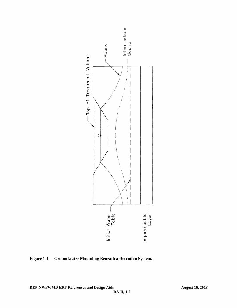
When runoff enters the retention basin, standing water in the basin begins to infiltrate. Water in the retention basin exits the basin in two distinct stages, either vertically (Stage One) through the basin bottom (unsaturated flow) or laterally (Stage Two) through the side slopes (saturated flow). One flow direction or the other will predominate depending on the height of the water table in relation to the bottom of the basin. The following paragraph briefly describes the two stages of infiltration and subsequent subsections present accepted methodologies for calculating infiltration rates and recovery times for unsaturated vertical (Stage One) and saturated lateral (Stage Two) flow. Initially, the subsurface conditions are assumed to be the seasonal high ground water table (SHGWT) below the basin bottom, and the soil above the SHGWT is unsaturated. When the water begins to infiltrate, it is driven downward in unsaturated flow by the combined forces of gravity and capillary action. The water penetrates deeper and deeper into the ground and fills the voids in the soil. Once the unsaturated soil below the basin becomes saturated, the water table "mounds" beneath the basin (Figure 1-1, below). At this time, saturation below the basin prevents further vertical movement and water exiting the basin begins to flow laterally. For successful design of retention basins, both the unsaturated and saturated infiltration must be accounted for and incorporated into the analysis.
1.2 Water Management District Sponsored Research on Retention Systems
In the early 1990’s, the St. Johns River Water Management District (SJRWMD) conducted full-scale hydrologic monitoring of retention basins in order to improve the design parameters and operational effectiveness of retention systems. This field data was used to evaluate and to recommend hydrogeologic characterization techniques and design methodologies for computing the time of percolation of impounded stormwater runoff. Although all of the retention basins selected for instrumentation were located within the Indian River Lagoon Basin of the SJRWMD where soil infiltration potential is somewhat limited, the results of the study and the design recommendations have state-wide applicability for similar areas where water table and soil conditions limit percolation. Copies of the report may be obtained from the SJRWMD
DEP-NWFWMD ERP References and Design Aids August 16, 2013 DA-II, 1-2
Figure 1-1 Groundwater Mounding Beneath a Retention System.

DEP-NWFWMD ERP References and Design Aids August 16, 2013 DA-II, 1-3
(request District Special Publication SJ93-SP10). The document also is available online at http://www.dep.state.fl.us/water/wetlands/erp/rules/guide.htm.
The study included design recommendations on field and laboratory methods of aquifer characterization and methodologies for computing recovery time. Acceptable methodologies for calculating retention basin recovery are presented in section 1.3, below, and recommended field and laboratory aquifer characterization testing methods are presented in section 1.4, below. These methodologies are based, in part, on the results in Special Publication SJ93-SP10.
1.3 Accepted Methodologies and Design Procedures for Retention Basin Recovery
3.1 Accepted Methodologies 1. Acceptable methodologies for calculating retention basin recovery are presented below in Table 1-1,
below. Vertical unsaturated flow methodologies are described in more detail in section 1.3.3 below and lateral saturated flow methodologies are presented in section 1.3.4 below.
Table 1-1. Accepted Methodologies for Retention Basin Recovery
Vertical Unsaturated Flow Lateral Saturated Flow
Green and Ampt Equation PONDS
Hantush Equation PONDFLOW
Horton Equation Modified MODRET
Darcy Equation
Holton Equation Several of these methodologies are available commercially in computer programs. The agency can neither endorse any program nor certify program results. If applicants wish to calculate retention basin recovery by hand, acceptable methodologies for vertical
unsaturated and lateral saturated flow are described in sections 1.3.3 and 1.3.5, below, respectively. A design example for each flow condition is presented below in section 1.5, below.
1.3.2 Design Procedures It is recommended that, unless the normal seasonal high water table is over 6 inches below the basin
bottom, unsaturated flow prior to saturated lateral mounding be conservatively ignored in recovery analysis. In other words, there should be no credit for soil storage immediately beneath the basin if the seasonal high water table is within 6 inches of the basin bottom. This is not an unrealistic assumption since the height of capillary fringe in fine sand is on the order of 6 inches and a partially mounded water table condition may be remnant from a previous storm event, especially during the wet season.
It is also recommended that the filling of the pond with the treatment volume be simulated as a "slug"
loading (i.e., treatment volume fills the pond within an hour).
DEP-NWFWMD ERP References and Design Aids August 16, 2013 DA-II, 1-4
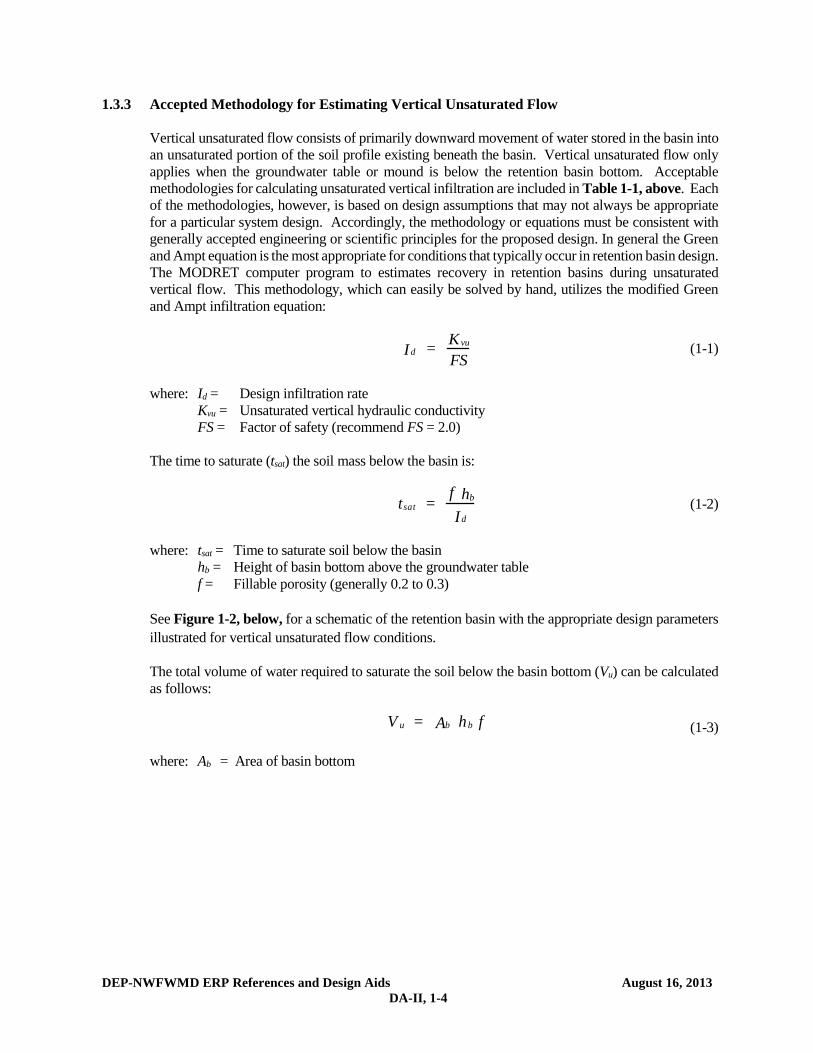
1.3.3 Accepted Methodology for Estimating Vertical Unsaturated Flow
Vertical unsaturated flow consists of primarily downward movement of water stored in the basin into an unsaturated portion of the soil profile existing beneath the basin. Vertical unsaturated flow only applies when the groundwater table or mound is below the retention basin bottom. Acceptable methodologies for calculating unsaturated vertical infiltration are included in Table 1-1, above. Each of the methodologies, however, is based on design assumptions that may not always be appropriate for a particular system design. Accordingly, the methodology or equations must be consistent with generally accepted engineering or scientific principles for the proposed design. In general the Green and Ampt equation is the most appropriate for conditions that typically occur in retention basin design. The MODRET computer program to estimates recovery in retention basins during unsaturated vertical flow. This methodology, which can easily be solved by hand, utilizes the modified Green and Ampt infiltration equation:
dI = vuKFS
(1-1)
where: Id = Design infiltration rate
Kvu = Unsaturated vertical hydraulic conductivity FS = Factor of safety (recommend FS = 2.0)
The time to saturate (tsat) the soil mass below the basin is:
satt = f bh
dI (1-2)
where: tsat = Time to saturate soil below the basin
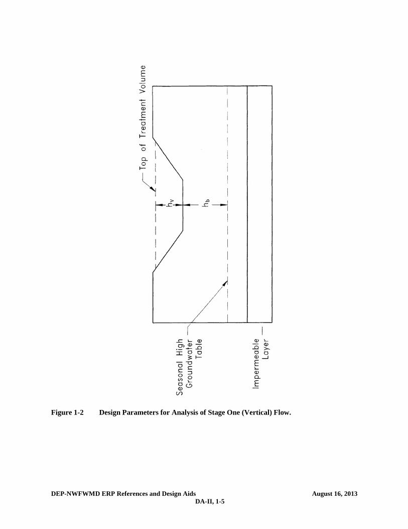
hb = Height of basin bottom above the groundwater table f = Fillable porosity (generally 0.2 to 0.3)
See Figure 1-2, below, for a schematic of the retention basin with the appropriate design parameters illustrated for vertical unsaturated flow conditions.
The total volume of water required to saturate the soil below the basin bottom (Vu) can be calculated as follows:
uV = bA bh f (1-3)
where: Ab = Area of basin bottom
DEP-NWFWMD ERP References and Design Aids August 16, 2013 DA-II, 1-5
Figure 1-2 Design Parameters for Analysis of Stage One (Vertical) Flow.
DEP-NWFWMD ERP References and Design Aids August 16, 2013 DA-II, 1-6
Likewise, the height of water required to saturate the soil below the basin bottom (hu) can be calculated using:
u bh = f h (1-4)
Recovery of the treatment storage will occur entirely under vertical unsaturated flow conditions when: (a) Treatment volume ≤ Vu ; or (b) Height of the treatment volume (hv) in the basin ≤ hu
If recovery of the treatment storage occurs entirely under vertical unsaturated conditions, analysis of the system for saturated lateral flow conditions will not be necessary.
This simplified approach is conservative because it does not consider the horizontal movement of water from the ground water mound that forms during this stage. In cases where the horizontal permeability is great, a more accurate estimate of the total vertical unsaturated flow can be obtained by using the Hantush equation. However, horizontal permeability of the unsaturated zone must be determined using an appropriate field or laboratory test consistent with generally accepted engineering or scientific principles.
A factor of safety (FS) of 2.0 is recommended to account for flow losses due to basin bottom siltation and clogging. For most sandy soils the fillable porosity (f) is approximately 0.2 to 0.3. The unsaturated vertical hydraulic conductivity (Kvu) can be measured using the field testing procedures or laboratory methods recommended in section 1.4, below.
A design example for utilizing the above methodology is presented below in section 1.5, below.
1.3.4 Accepted Methodologies for Lateral Saturated Flow
If the ground water mound is at or above the basin bottom, the rate of water level decline in the basin is directly proportional to the rate of mound recession in the saturated aquifer. The Simplified Analytical Method, PONDFLOW, and Modified MODRET methodologies are generally acceptable for retention basin recovery analysis under lateral saturated flow conditions. These models are all similar in that the receiving aquifer system is idealized as a laterally infinite, single-layered, homogenous, isotropic water table aquifer of uniform thickness, with a horizontal water table prior to hydraulic loading. If these assumptions are not consistent with site conditions, a more appropriate model consistent with generally accepted engineering and scientific principles will be required.
All of the accepted models require input values for the pond dimensions, retained stormwater runoff volume, and the following set of aquifer parameters: • Thickness or elevation of base of mobilized (or effective) aquifer • Weighted horizontal hydraulic conductivity of mobilized aquifer • Fillable porosity of mobilized aquifer • Ambient water table elevation which, for design purposes is usually the normal seasonal high
water table In addition, to these one-layered, uniform aquifer idealization models accepted above, more
complicated fully three dimensional models with multiple layers (such as MODFLOW) may be used.
DEP-NWFWMD ERP References and Design Aids August 16, 2013 DA-II, 1-7
In order to use such three dimensional models, however, much more field data is necessary to characterize the three dimensional nature of the aquifer.
A brief description of each of the models recommended in Special Publication SJ93-SP10 is provided
below. The reader is encouraged to consult the Special Publication for a more detailed description. MODRET/Modified MODRET MODRET is a methodology developed for the Southwest Florida Water Management. The saturated
analysis module of MODRET is essentially a pre- and post-processor for the USGS three-dimensional ground water flow model MODFLOW. The MODRET model also has the capability to calculate unsaturated vertical flow from retention basins using the Green and Ampt equation. Unsaturated flow takes place prior to the ground water mound intersecting the basin bottom.
The input parameters in the MODRET pre-processor are use to create MODFLOW input files. After
the MODFLOW program is executed, the MODRET post-processor extracts and prints the relevant information from the MODFLOW output files. MODRET allows the user to input time-varying recharge (such as a hydrograph from a storm event) and calculate saturated flow out of the basin during recharge (i.e., a storm event).
During the study presented in Special Publication SJ93-SP10, it was discovered that the MODRET
model was producing unstable MODFLOW solutions when modeling the recovery of some of the sites. This problem generally occurs when one or a combination of the following is true: • The pond dimensions are relatively large (greater than 100 feet) • The aquifer is relatively thin (less than 5 feet) • The horizontal hydraulic conductivity is relatively low (less than 5 ft/day)
Upon further review, the MODRET model was modified in the study to correct this instability
problem by changing the head change criterion for convergence to 0.001 ft from 0.01 ft. The original MODRET model with this modification is therefore referred to as "Modified MODRET."
PONDFLOW PONDFLOW is a retention recovery computer model that is similar to MODRET in that it is uses a
finite difference numerical technique to approximate the time varying ground water profile adjacent to the basin. Also, like MODRET it can accommodate a time-varying recharge to the pond, account for seepage during the storm, and also calculates vertical unsaturated flow using Darcy's Equation.
1.3.5 Methodology for Analyzing Recovery by Lateral Saturated Flow by Hand The MODFLOW groundwater flow computer model developed by the U.S. Geological Survey can
be used to generate a series of dimensionless curves to predict retention basin recovery under lateral saturated flow (Stage Two) conditions. The dimensionless parameters can be expressed as:
xF = 2W
4 HK D t (1-5)
yF = ch
TH (1-6)
DEP-NWFWMD ERP References and Design Aids August 16, 2013 DA-II, 1-8
where: Fx = Dimensionless parameter representing physical and hydraulic characteristics of the
retention basin and effective aquifer system (x-axis) Fy = Dimensionless parameter representing percent of water level decline below a
maximum level (y-axis) W = Average width of the retention basin, midway between basin bottom and water level
at time t (ft) KH = Average horizontal hydraulic conductivity (ft/day) D = Average saturated thickness of the aquifer (ft) t = Cumulative time since saturated lateral (Stage Two) flow started (days) hc = Height of water in the basin above the initial ground water table at time t (ft) HT = Height of water in the basin above the initial ground water table at the start of saturated
lateral (Stage Two) flow (ft) The average saturated thickness of the aquifer (D) can be expressed as:
D = H + ch
2 (1-7) where: H = Initial saturated thickness of the aquifer (ft) The height of water in the basin above the initial groundwater table at the start of saturated lateral
(Stage Two) flow (HT) is: 2hhH bT += (1-8) where: h2 = Height of water in the basin above the basin bottom at the start of saturated
lateral (Stage Two) flow (ft) Figure 1-3, below, contains an illustration of the design parameters for analysis of saturated lateral
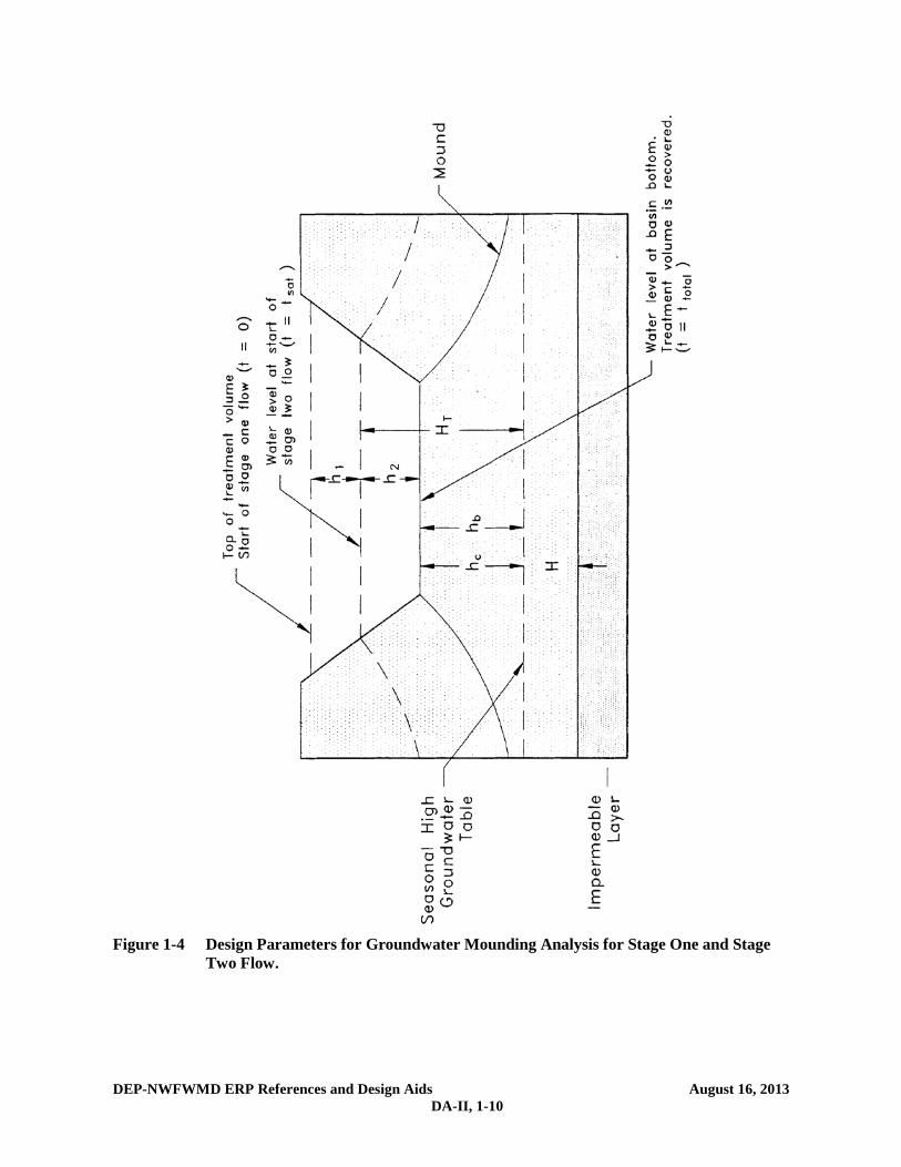
(Stage Two) flow conditions. The design parameters for a retention system utilizing both unsaturated vertical (Stage One) and saturated lateral (Stage Two) flow is represented in Figure 1-4, below.
The equation for Fx can be rearranged to solve for the time (t) to recover the remaining treatment volume under saturated lateral (Stage Two) flow:
t = 2W
4 HK D x2F
(1-9)

DEP-NWFWMD ERP References and Design Aids August 16, 2013 DA-II, 1-9
Figure 1-3 Design Parameters for Groundwater Mounding Analysis for Stage Two (Lateral)
Flow.
DEP-NWFWMD ERP References and Design Aids August 16, 2013 DA-II, 1-10
Figure 1-4 Design Parameters for Groundwater Mounding Analysis for Stage One and Stage Two Flow.
DEP-NWFWMD ERP References and Design Aids August 16, 2013 DA-II, 1-11
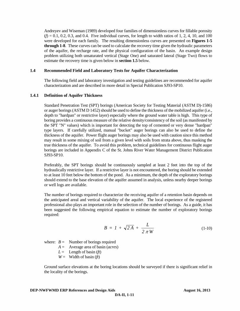
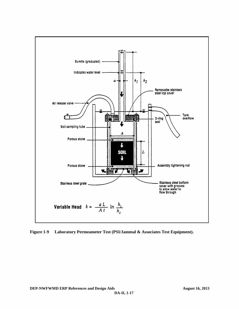
Andreyev and Wiseman (1989) developed four families of dimensionless curves for fillable porosity (f) = 0.1, 0.2, 0.3, and 0.4. Five individual curves, for length to width ratios of 1, 2, 4, 10, and 100 were developed for each family. The resulting dimensionless curves are presented on Figures 1-5 through 1-8. These curves can be used to calculate the recovery time given the hydraulic parameters of the aquifer, the recharge rate, and the physical configuration of the basin. An example design problem utilizing both unsaturated vertical (Stage One) and saturated lateral (Stage Two) flows to estimate the recovery time is given below in section 1.5 below.
1.4 Recommended Field and Laboratory Tests for Aquifer Characterization
The following field and laboratory investigation and testing guidelines are recommended for aquifer characterization and are described in more detail in Special Publication SJ93-SP10.
1.4.1 Definition of Aquifer Thickness Standard Penetration Test (SPT) borings (American Society for Testing Material (ASTM D)-1586)
or auger borings (ASTM D 1452) should be used to define the thickness of the mobilized aquifer (i.e., depth to "hardpan" or restrictive layer) especially where the ground water table is high. This type of boring provides a continuous measure of the relative density/consistency of the soil (as manifested by the SPT "N" values) which is important for detecting the top of cemented or very dense "hardpan" type layers. If carefully utilized, manual "bucket" auger borings can also be used to define the thickness of the aquifer. Power flight auger borings may also be used with caution since this method may result in some mixing of soil from a given level with soils from strata above, thus masking the true thickness of the aquifer. To avoid this problem, technical guidelines for continuous flight auger borings are included in Appendix C of the St. Johns River Water Management District Publication SJ93-SP10.
Preferably, the SPT borings should be continuously sampled at least 2 feet into the top of the
hydraulically restrictive layer. If a restrictive layer is not encountered, the boring should be extended to at least 10 feet below the bottom of the pond. As a minimum, the depth of the exploratory borings should extend to the base elevation of the aquifer assumed in analysis, unless nearby deeper borings or well logs are available.
The number of borings required to characterize the receiving aquifer of a retention basin depends on the anticipated areal and vertical variability of the aquifer. The local experience of the registered professional also plays an important role in the selection of the number of borings. As a guide, it has been suggested the following empirical equation to estimate the number of exploratory borings required:
B = 1 + 2 A + L2 Wπ
(1-10)
where: B = Number of borings required A = Average area of basin (acres) L = Length of basin (ft) W = Width of basin (ft) Ground surface elevations at the boring locations should be surveyed if there is significant relief in
the locality of the borings.
DEP-NWFWMD ERP References and Design Aids August 16, 2013 DA-II, 1-12
Figure 1-5 Dimensionless Curves Relating Basin Design Parameters to Basin Water Level in a Rectangular Retention Basin Over an Unconfined Aquifer (f = 0.1).

DEP-NWFWMD ERP References and Design Aids August 16, 2013 DA-II, 1-13
Figure 1-6 Dimensionless Curves Relating Basin Design Parameters to Basin Water Level in a Rectangular Retention Basin Over an Unconfined Aquifer (f = 0.2).

DEP-NWFWMD ERP References and Design Aids August 16, 2013 DA-II, 1-14
Figure 1-7 Dimensionless Curves Relating Basin Design Parameters to Basin Water Level in a
Rectangular Retention Basin Over an Unconfined Aquifer (f = 0.3).

DEP-NWFWMD ERP References and Design Aids August 16, 2013 DA-II, 1-15
Figure 1-8 Dimensionless Curves Relating Basin Design Parameters to Basin Water Level in a
Rectangular Retention Basin Over an Unconfined Aquifer (f = 0.4).

DEP-NWFWMD ERP References and Design Aids August 16, 2013 DA-II, 1-16
1.4.2 Estimated Normal Seasonal High Ground Water Table
In estimating the normal seasonal high ground water table (SHGWT), the contemporaneous measurements of the water table are adjusted upward or downward taking into consideration numerous factors, including: antecedent rainfall, redoximorphic features (i.e., soil mottling), stratigraphy (including presence of hydraulically restrictive layers), vegetative indicators, effects of development, and hydrogeologic setting. The application of these adjustments requires considerable experience. The SHGWT shall be determined utilizing generally accepted geotechnical and soil science principles. The October 27, 1997 USDA NRCS “Depth to Seasonal High Saturation and Seasonal Inundation” memorandum provides such principles and methodologies for determining SHGWT.
In general, the measurement of the depth to the ground water table is less accurate in SPT borings when drilling fluids are used to maintain an open borehole. Therefore, when SPT borings are drilled, it may be necessary to drill an auger boring adjacent to the SPT to obtain a more precise stabilized water table reading. In poorly drained soils, the auger boring should be left open long enough (at least 24 hours) for the water table to stabilize in the open hole.
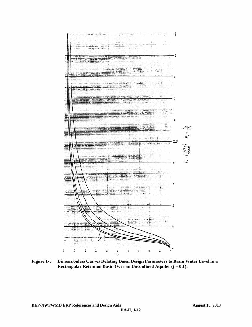
1.4.3 Estimation of Horizontal Hydraulic Conductivity of Aquifer The following hydraulic conductivity tests are recommended for retention systems: a) Laboratory hydraulic conductivity test on undisturbed sample (Figure 1-9, below). b) Uncased or fully screened auger hole using the equation on Figure 1-10, below. c) Cased hole with uncased or screened extension with the base of the extension at least one
foot above the confining layer (Figure 1-11, below). d) Pump test or slug test, when accuracy is important and hydrostratigraphy is conductive to
such a test method.
Of the above methods, the most cost effective is the laboratory permeameter test on an undisturbed horizontal sample. However, it becomes difficult and expensive to obtain undisturbed hydraulic conductivity tube samples under the water table or at depths greater than 5 feet below ground surface. In such cases -- where the sample depth is over 5 feet below ground surface or below the water table -- it is more appropriate to use the in situ uncased or fully screened auger hole method (Figure 1-10, below) or the cased hole with uncased or screened extension (Figure 1-11, below).
The main limitation of the laboratory permeameter test on a tube sample is that it represents the hydraulic conductivity at a point in the soil profile which may or may not be representative of the entire thickness of the mobilized aquifer. In most cases, the sample is retrieved at a depth of 2 to 3 feet below ground surface where the soil is most permeable, while the mobilized aquifer depth may be 5 to 6 feet. It is therefore important to use some judgment and experience in reviewing the soil profile to estimate the weighted hydraulic conductivity of the mobilized aquifer. It is not practical or economical to obtain and test permeability tubes at each point in the soil profile where there is a change in density, degree of cementation, or texture. Some judgment and experience must therefore
DEP-NWFWMD ERP References and Design Aids August 16, 2013 DA-II, 1-17
Figure 1-9 Laboratory Permeameter Test (PSI/Jammal & Associates Test Equipment).

DEP-NWFWMD ERP References and Design Aids August 16, 2013 DA-II, 1-18
Figure 1-10 Field Hydraulic Conductivity Test: Uncased or Fully Screened Auger Hole, Constant
Head.

DEP-NWFWMD ERP References and Design Aids August 16, 2013 DA-II, 1-19
Figure 1-11 Field Hydraulic Conductivity Test: Cased Hole with Uncased or Screened Extension.
DEP-NWFWMD ERP References and Design Aids August 16, 2013 DA-II, 1-20
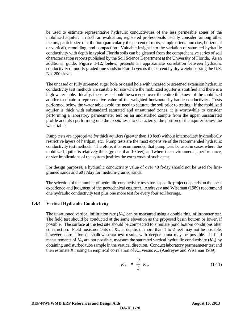
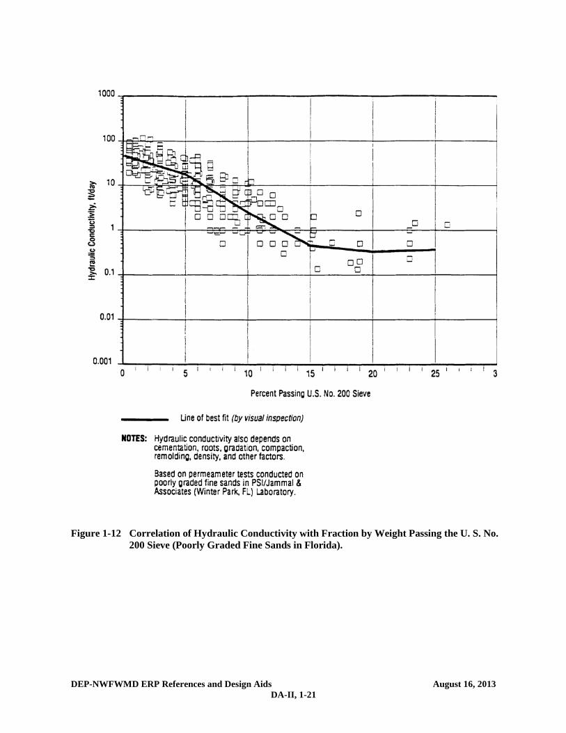
be used to estimate representative hydraulic conductivities of the less permeable zones of the mobilized aquifer. In such an evaluation, registered professionals usually consider, among other factors, particle size distribution (particularly the percent of roots, sample orientation (i.e., horizontal or vertical), remolding, and compaction. Valuable insight into the variation of saturated hydraulic conductivity with depth in typical Florida soils can be gleaned from the comprehensive series of soil characterization reports published by the Soil Science Department at the University of Florida. As an additional guide, Figure 1-12, below, presents an approximate correlation between hydraulic conductivity of poorly graded fine sands in Florida versus the percent by dry weight passing the U.S. No. 200 sieve.
The uncased or fully screened auger hole or cased hole with uncased or screened extension hydraulic
conductivity test methods are suitable for use where the mobilized aquifer is stratified and there is a high water table. Ideally, these tests should be screened over the entire thickness of the mobilized aquifer to obtain a representative value of the weighted horizontal hydraulic conductivity. Tests performed below the water table avoid the need to saturate the soil prior to testing. If the mobilized aquifer is thick with substandard saturated and unsaturated zones, it is worthwhile to consider performing a laboratory permeameter test on an undisturbed sample from the upper unsaturated profile and also performing one the in situ tests to characterize the portion of the aquifer below the water table.
Pump tests are appropriate for thick aquifers (greater than 10 feet) without intermediate hydraulically
restrictive layers of hardpan, etc. Pump tests are the most expensive of the recommended hydraulic conductivity test methods. Therefore, it is recommended that pump tests be used in cases where the mobilized aquifer is relatively thick (greater than 10 feet), and where the environmental, performance, or size implications of the system justifies the extra costs of such a test.
For design purposes, a hydraulic conductivity value of over 40 ft/day should not be used for fine-
grained sands and 60 ft/day for medium-grained sands. The selection of the number of hydraulic conductivity tests for a specific project depends on the local
experience and judgment of the geotechnical engineer. Andreyev and Wiseman (1989) recommend one hydraulic conductivity test plus one more test for every four soil borings.
1.4.4 Vertical Hydraulic Conductivity The unsaturated vertical infiltration rate (Kvu) can be measured using a double ring infiltrometer test.
The field test should be conducted at the same elevation as the proposed basin bottom or lower, if possible. The surface at the test site should be compacted to simulate pond bottom conditions after construction. Field measurements of Kvu at depths of more than 1 to 2 feet may not be possible, however, correlation of shallow strata test results with deeper strata may be possible. If field measurements of Kvu are not possible, measure the saturated vertical hydraulic conductivity (Kvs) by obtaining undisturbed tube sample in the vertical direction. Conduct laboratory permeameter test and then estimate Kvu using an empirical correlation of Kvu versus Kvs (Andreyev and Wiseman 1989):
vu vsK = 23
K (1-11)
DEP-NWFWMD ERP References and Design Aids August 16, 2013 DA-II, 1-21
Figure 1-12 Correlation of Hydraulic Conductivity with Fraction by Weight Passing the U. S. No.
200 Sieve (Poorly Graded Fine Sands in Florida).

DEP-NWFWMD ERP References and Design Aids August 16, 2013 DA-II, 1-22
1.4.5 Estimation of Fillable Porosity In Florida, the receiving aquifer system for retention basins predominantly comprises poorly graded
(i.e., relatively uniform particle size) fine sands. In these materials, the water content decreases rather abruptly with the distance above the water table and they therefore have a well-defined capillary fringe.
Unlike the hydraulic conductivity parameter, the fillable porosity value of the poorly graded fine sand
aquifers in Florida are in a much narrower range (20 to 30 percent), and can therefore be estimated with much more reliability. For fine sand aquifers, it is therefore recommended that a fillable porosity in the range 20 to 30 percent be used in infiltration calculations. The higher values of fillable porosity will apply to the well- to excessively-drained, hydrologic group "A" fine sands, which are generally deep, contain less than 5 percent by weight passing the U.S. No. 200 (0.074 mm) sieve, and have a natural moisture content of less than 5 percent. No specific field or laboratory testing requirements is recommended to estimate this parameter.
1.5 Design Example for Retention Basin Recovery
The following design example is for estimating retention basin recovery by hand utilizing the methodologies in sections 1.3.3 and 1.3.5, above.
Given: Commercial project discharging to Class III waters Drainage area = 3.75 acres Percent impervious = 40% Off-site drainage area = 0 acres Off-line treatment f = 0.30; Kvs = 2 ft/day; KH = 10 ft/day; FS = 2.0 Basin bottom elevation = 20.0 feet Seasonal high groundwater table elevation = 17.0 feet Impervious layer elevation = 14.0 feet Rectangular retention basin with bottom dimensions of length = 100 ft and width = 50 ft
The proposed retention basin has the following stage-storage relationship:
Stage (ft)
Storage (ft3)
20.00 0 20.25 1278 20.50 2615 20.75 4011 21.00 5468 21.25 6988
Objective: Calculate the time to recover the treatment volume.
Design Calculations
Part I. Calculate the Treatment Volume and the Height of the Treatment Volume in the Basin
DEP-NWFWMD ERP References and Design Aids August 16, 2013 DA-II, 1-23
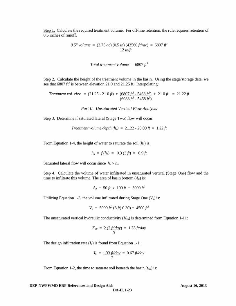
Step 1. Calculate the required treatment volume. For off-line retention, the rule requires retention of 0.5 inches of runoff.
0.5" volume = (3.75 ac) (0.5 in) (43560 ft2/ac) = 6807 ft3
12 in/ft
Total treatment volume = 6807 ft3
Step 2. Calculate the height of the treatment volume in the basin. Using the stage/storage data, we see that 6807 ft3 is between elevation 21.0 and 21.25 ft. Interpolating:
Treatment vol. elev. = (21.25 - 21.0 ft) x (6807 ft3 - 5468 ft3) + 21.0 ft = 21.22 ft
(6988 ft3 - 5468 ft3)
Part II. Unsaturated Vertical Flow Analysis
Step 3. Determine if saturated lateral (Stage Two) flow will occur.
Treatment volume depth (hv) = 21.22 - 20.00 ft = 1.22 ft
From Equation 1-4, the height of water to saturate the soil (hu) is:
hu = f (hb) = 0.3 (3 ft) = 0.9 ft
Saturated lateral flow will occur since hv > hu Step 4. Calculate the volume of water infiltrated in unsaturated vertical (Stage One) flow and the time to infiltrate this volume. The area of basin bottom (Ab) is:
Ab = 50 ft x 100 ft = 5000 ft2
Utilizing Equation 1-3, the volume infiltrated during Stage One (Vu) is:
Vu = 5000 ft2 (3 ft) 0.30) = 4500 ft3
The unsaturated vertical hydraulic conductivity (Kvu) is determined from Equation 1-11:
Kvu = 2 (2 ft/day) = 1.33 ft/day
3
The design infiltration rate (Id) is found from Equation 1-1:
Id = 1.33 ft/day = 0.67 ft/day 2
From Equation 1-2, the time to saturate soil beneath the basin (tsat) is:

DEP-NWFWMD ERP References and Design Aids August 16, 2013 DA-II, 1-24
tsat = (3 ft)(0.30) = 1.34 days 0.67 ft/day
Part III. Saturated Lateral Flow Analysis
Step 5. Calculate the remaining treatment volume to be recovered under saturated lateral (Stage Two) flow conditions.
Remaining volume to be infiltrated under saturated lateral flow = 6807 - 4500 = 2307 ft3
Calculate the elevation of treatment volume at the start of saturated lateral flow by interpolating: Treatment volume elev. = (20.50 - 20.25 ft) x (2307 ft3 - 1278 ft3) + 20.25 ft = 20.44 ft at start of saturated (2615 ft3 - 1278 ft3) lateral flow
Step 6. Calculate Fy and Fx When the treatment volume is recovered (time t = tTotal) the water level is at the basin bottom. Hence, the height of the water level above the initial groundwater table (hc) will be equal to hb.
hc = hb = 3 ft (at t = tTotal)
The height of water in the basin at the start of saturated lateral flow (h2) is:
h2 = 20.44 - 20.0 = 0.44 ft
From Equation 1-8:
HT = hb + h2 = 3.0 + 0.44 = 3.44 ft
Fy is determined from Equation 1-6:
Fy = 3 ft = 0.87 3.44 ft
When the water level is at the basin bottom (time t = tTotal) the basin length (L) = 100 ft and the basin width (W) = 50 ft.
Basin length to width ratio (L/W) = 100 ft = 2
50 ft
Determine Fx.
From Figure 1-7; Fx = 4.0 (for f = 0.3, L/W = 2, and Fy = 0.87)

DEP-NWFWMD ERP References and Design Aids August 16, 2013 DA-II, 1-25
Step 7. Calculate the time to recover the remaining treatment volume under saturated lateral flow.
H = 17.0 - 14.0 = 3.0 ft
The average saturated thickness (D) can be found from Equation 1-7:
D = H + hc = 3.0 + 3.0 = 4.5 ft 2 2
The time (t) to recover the remaining treatment volume under lateral saturated flow conditions is determined from Equation 1-9:
t = (50 ft)2 = 0.87 days
(4) (10 ft/day) (4.5 ft) (4.0)2
Part IV. Calculate Total Recovery Time
Step 8. Total time to recover the treatment volume (tTotal) equals the time to recover during unsaturated vertical flow plus the time to recover under lateral saturated conditions.
Total recovery time (tTotal) = 1.34 days + 0.87 days = 2.21 days or 53 hours
Therefore, the design meets the 72 hour recovery time criteria.
DEP-NWFWMD ERP References and Design Aids August 16, 2013 DA-II, 2-1
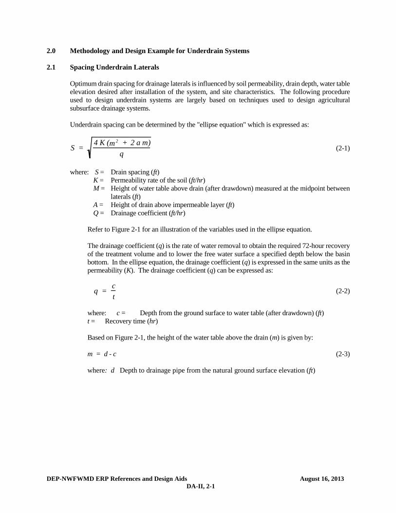
2.0 Methodology and Design Example for Underdrain Systems 2.1 Spacing Underdrain Laterals Optimum drain spacing for drainage laterals is influenced by soil permeability, drain depth, water table
elevation desired after installation of the system, and site characteristics. The following procedure used to design underdrain systems are largely based on techniques used to design agricultural subsurface drainage systems.
Underdrain spacing can be determined by the "ellipse equation" which is expressed as:
S = 4 K ( 2m + 2 a m)
q (2-1)
where: S = Drain spacing (ft) K = Permeability rate of the soil (ft/hr) M = Height of water table above drain (after drawdown) measured at the midpoint between
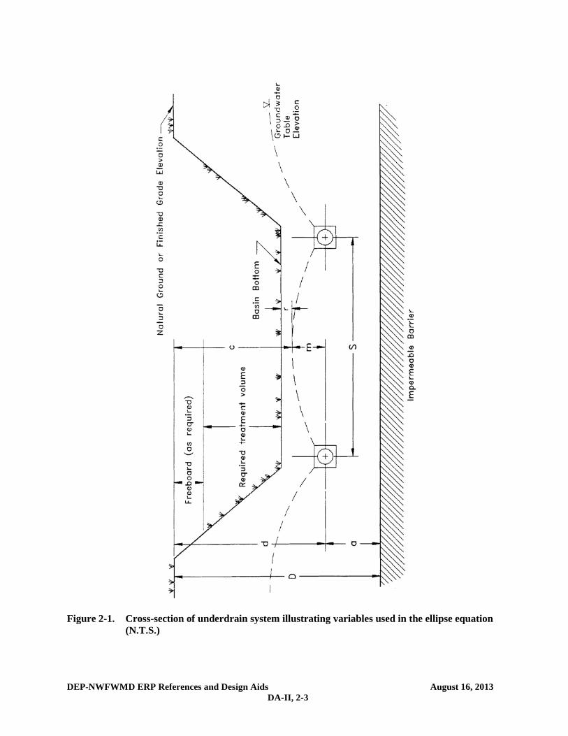
laterals (ft) A = Height of drain above impermeable layer (ft) Q = Drainage coefficient (ft/hr) Refer to Figure 2-1 for an illustration of the variables used in the ellipse equation. The drainage coefficient (q) is the rate of water removal to obtain the required 72-hour recovery
of the treatment volume and to lower the free water surface a specified depth below the basin bottom. In the ellipse equation, the drainage coefficient (q) is expressed in the same units as the permeability (K). The drainage coefficient (q) can be expressed as:
q = ct
(2-2)
where: c = Depth from the ground surface to water table (after drawdown) (ft) t = Recovery time (hr)
Based on Figure 2-1, the height of the water table above the drain (m) is given by:
m = d - c (2-3) where: d Depth to drainage pipe from the natural ground surface elevation (ft)

DEP-NWFWMD ERP References and Design Aids August 16, 2013 DA-II, 2-2
The height of the drain above the impermeable barrier (a) is: a = D - d (2-4) where: D = Depth to impermeable layer from the natural ground surface elevation (ft) When there is no impermeable barrier present, the depth to the impermeable layer (D) should be assumed at a depth equal to twice the drain depth (d). The ellipse equation is based on steady state conditions and the assumption that ground water inflow from outside the area is slight. For this reason the use of the ellipse equation should be limited to conditions in which: (a) The hydraulic gradient of the undisturbed water table is one percent (0.01 feet per foot)
or less. Under these conditions there is likely to be very little ground water flow or movement from outside the system.
(b) The site is underlain by a impermeable barrier at relatively shallow depths (twice the depth
of the drain (d) or less) which restricts vertical flow and forces the percolating water to flow horizontally toward the drain.
(c) A gravel envelope surrounds the perforated drainage pipes so that flow restrictions into
the drain are minimized. (d) The height of drain above impermeable layer (a) is less than or equal to the depth to the
drainage pipe (d). 2.2 Length of Underdrain Required and Basin Dimensions It is desirable to keep both the bottom and sides of the detention area dry. To maintain a dry basin
bottom, the District recommends the distance between the basin bottom and water table after drawdown be at least 6 inches (see Figure 2-1). Maintaining r ≥ 6 inches will ensure that the floor of the basin is above the ground water table capillary zone.
If the side slope and shape of the detention basin are known, it is possible to determine the dimensions
of the basin and the exact length of drain pipe needed. The area (AL) served by each lateral in a rectangular basin is given by (see Figure 2-2):
AL = S (L + S) (2-5) where: AL = Area served by each lateral (ft2) L = Length of lateral (ft)
DEP-NWFWMD ERP References and Design Aids August 16, 2013 DA-II, 2-3
Figure 2-1. Cross-section of underdrain system illustrating variables used in the ellipse equation
(N.T.S.)

DEP-NWFWMD ERP References and Design Aids August 16, 2013 DA-II, 2-4
Figure 2-2. Top view of underdrain system illustrating variables used in the ellipse equation
(N.T.S.)
DEP-NWFWMD ERP References and Design Aids August 16, 2013 DA-II, 2-5
The total area served by all the laterals (ATL) is: ATL = AL N (2-6) where: N = Number of laterals The top area of the detention basin (ABT) can be expressed as: ABT = DPAR DPER (2-7) where: ABT = Top area of the detention basin (ft2) DPAR = Distance of top of basin in the direction parallel to the laterals (ft) DPER = Distance of top of basin in the direction perpendicular to the laterals (ft) Setting the total area served by the laterals (ATL) so that it is equal to the area of the detention basin as measured from the top of bank dimensions (ABT), will ensure that both the bottom and sides of the basin remain dry between storm events. In this case the criteria for the lateral spacings and the top dimensions of the basin are determined as follows:
Lateral Length : L + S ≥ PARD (2-8)
Lateral Spacing : S (N) ≥ PERD (2-9)
Lateral Side Offset Distance : Offset ≤ S2
(2-10)
Top Area: DPAR (DPER) ≤ ATL (2-11) Given the lateral spacing (S) and two of the three variables L, DPAR, or DPER, the designer can solve for the unknown variable using the equations in this section. An example problem for designing an underdrain system is given in section 27.5. 2.3 Drain Size The discharge from a drain may be found by the following formula (SCS 1973):
rQ =
q S L + S2
CF (2-12) where: Qr = Relief drain discharge (cfs) S = Drain spacing (ft) L = Drain length (ft) q = Drainage coefficient (in/hr) CF = Conversion factor = 43200 Subsurface drains ordinarily are not designed to flow under pressure. The hydraulic gradient is considered to be parallel with the grade line of the underdrain. The flow in the drain is considered to be open-channel flow.

DEP-NWFWMD ERP References and Design Aids August 16, 2013 DA-II, 2-6
The size conduit required for a given capacity is dependent on the hydraulic gradient and the roughness coefficient (n) of the drain. Commonly used materials have n values ranging from about 0.011 for good quality smooth plastic pipe to about 0.025 for corrugated metal. When determining the size of drain required for a particular situation the n value of the product to be used must be known. This information will normally be available from the manufacturer. The diameter pipe required for a given capacity, hydraulic gradient, and four different n values may be determined from Figures 2-3, 2-4, 2-5, and 2-6. The area to the right of the broken line in the charts indicates conditions where the velocity of flow is expected to be less than 2.0 ft/sec. Lower velocities may present a problem with siltation in areas of fine soils. 2.4 Sizing of Drains Within the System The previous discussion on drain size deals with the problem of selecting the proper size for a drain at a specific point in the stormwater system. In drainage systems with laterals and mains, the variation of flow within a single line may be great enough to warrant changing size in the line. This is often the case in long drains or system with numerous laterals. The example problem in section 27.5 illustrates a method for such a design. 2.5 Example Design Calculations for Underdrain Systems Given: Desired depth of the treatment volume in the basin = 3 feet Desired basin freeboard = 1 ft 4" minimum pipe diameter 3" gravel envelope on each side of the drainage pipes Minimum distance between basin bottom and top of the gravel envelope = 2 feet = m + r Depth from natural ground to impermeable barrier = 7.5 feet Area of basin (measured from top of treatment volume) = 7260 ft2 Maximum top dimension of basin perpendicular to drainage laterals = 30 feet K = 1.0 ft/hr Slope of laterals = 0.2% n = 0.015 Safety factor = 2.0 "T" shaped drainage network (similar to Figure 2-2) Objective: Design an underdrain system to lower the water level to a level 6" below the basin bottom within 72 hours. Design Calculations: Step 1. Calculate the required drain spacing. First determine the depth to the drain line from natural ground surface (d) from the following relationship:
Depth to the drain line from = Depth of treatment volume in the basin + depth of natural ground surface (d) freeboard + depth of soil between basin floor and envelope + depth of gravel envelope + drain radius
d = 3 ft + 1 ft + 2 ft + 3 in + 2 in = 6.42 ft 12 in/ft 12 in/ft Determine the height of the drain above the impermeable layer (a) by utilizing Equation 2-4:

DEP-NWFWMD ERP References and Design Aids August 16, 2013 DA-II, 2-7
a = D - d = 7.5 - 6.42 = 1.08 ft
Depth to water table after drawdown (c) = treatment volume depth + freeboard depth + r
c = 3 ft + 1 ft + 6 in = 4.5 ft 12 in/ft From Equation 2-3:
m = d - c = 6.42 ft - 4.5 ft = 1.92 ft Determine the drainage coefficient (q) from Equation 2-2 with t = 36 hrs to incorporate a safety factor of 2 (i.e., 72/2 = 36):
q = c = 4.5 ft = 0.125 ft/hr = 1.5 in/hr t 36 hr The spacing (S) is determined from Equation 2-1:
( ) ( ) ( ) ( )[ ] fthrft
ftftfthrftS 8.15/125.0
92.108.1292.1/0.14 2
=+
=
Determine the number of laterals (N) utilizing Equation 2-9:
5.18.15
30≥≥
ftftN
Since the laterals should be located no farther than S/2 from the top of the basin, use two laterals spaced 15 ft apart and located 5 ft inside the top of basin. The two laterals will be connected to a main line with an outlet pipe intersecting at the midpoint of the main line. Step 2. Calculate the length of the laterals. Use Equation 2-11 with ABT = ATL:
ftftftDPAR 242
307260 2
==
Find the length of each lateral (L) from Equation 2-8:
ftftftL 22715242 =−= Step 3. Size the drainage laterals. The flow per lateral (Qr) is found from Equation 2-12:
rQ = (1.5 inch/hr) 15 ft 227 ft + 152
ft
143200
= 0.122 cfs
DEP-NWFWMD ERP References and Design Aids August 16, 2013 DA-II, 2-8
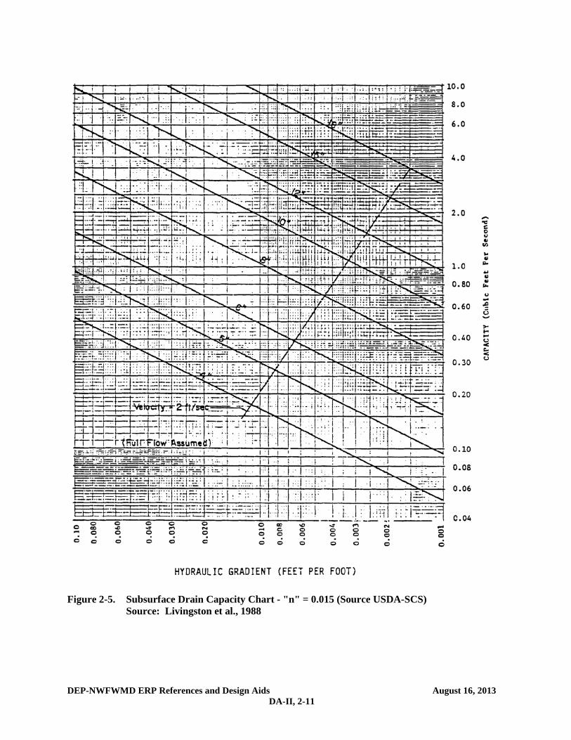
From Figure 2-5 with slope = 0.002 and n = 0.015, the capacity of a 4" pipe is 0.074 cfs. Since this is less than the flow rate that each lateral must convey, a 4" drain will not be sufficient for the entire length of the lateral and the size will have to be increased. Start the design process at the upper end of the drain using a minimum size of 4 inches. First, compute the distance that the drain would carry the flow on the assumed grade. The accretion per 100 would be:
cfsftft
cfs 054.0100/227
122.0=
The distance (in 100-foot sections) down gradient that a 4" drain would be adequate is:
( )pipe4"ofsectionsfoot10038.1054.0074.0
−=cfscfs
The 4" drain pipe is adequate for 135 feet of line. Continue these calculations for the next size pipe (5-inch) which has a maximum capacity of 0.13 cfs (from Figure 2-5).
( )pipe5"ofsectionsfoot10042.2055.013.0
−=cfs
cfs
The 5" drain would be adequate for 242 feet. Of this 242 feet, 138 would be 4" drain; and the remaining 104 feet would be 5" pipe. Since the total length required for each lateral is 227 feet, the amount of 5" drain needed is:
227 ft - 138 ft = 89ft of 5" drain per lateral
In summary, each lateral should contain 138 ft of 4" drain and 89 ft of 5" drain, although practical applications might consider 5" drain for the entire 227 ft. Step 4. Size the main and outlet lines. Assume the outlet intersects the main line at the midpoint. With only two laterals in the system, the main will not intersect any other laterals before reaching the outlet. Therefore, a 5" drain 10 feet in length on either side of the outlet will be sufficient for the main line.
Flow in the outlet = 0.122 cfs per lateral x 2 laterals = 0.244 cfs From Figure 2-5, with slope = 0.002 and n = 0.015; a flow of 0.244 cfs is greater than the capacity of a 6" but less than the capacity of a 8" drain. Therefore, use 8" drain for the outlet.

DEP-NWFWMD ERP References and Design Aids August 16, 2013 DA-II, 2-9
Figure 2-3. Subsurface Drain Capacity Chart - "n" = 0.011 (Source USDA-SCS) Source: Livingston et al., 1988

DEP-NWFWMD ERP References and Design Aids August 16, 2013 DA-II, 2-10
Figure 2-4. Subsurface Drain Capacity Chart - "n" = 0.013 (Source USDA-SCS) Source: Livingston et al., 1988
DEP-NWFWMD ERP References and Design Aids August 16, 2013 DA-II, 2-11
Figure 2-5. Subsurface Drain Capacity Chart - "n" = 0.015 (Source USDA-SCS) Source: Livingston et al., 1988

DEP-NWFWMD ERP References and Design Aids August 16, 2013 DA-II, 2-12
Figure 2-6. Subsurface Drain Capacity Chart - "n" = 0.025 (Source USDA-SCS) Source: Livingston et al., 1988
DEP-NWFWMD ERP References and Design Aids August 16, 2013 DA-II, 3-1
3.0 Methodology and Design Example for Wet Detention Systems 3.1 Calculating Permanent Pool Volumes
The residence time of a pond is defined as the average time required to renew the water volume (permanent pool volume) in the pond and can be expressed as:
RT = PPVFR
(3-1)
where: RT = Residence time (days) PPV = Permanent Pool Volume (ac-ft) FR = Average Flow Rate (ac-ft/day)
Solving Equation 3-1 for the permanent pool volume (PPV) gives:
PPV = (RT) (FR) (3-2)
The average flow rate (FR) during the wet season (June - September) can be expressed by:
FR = DA C R
WS (3-3)
where: DA = Drainage area to pond (ac) C = Runoff coefficient (see Table 3-1, below, for a list of recommended values for C) R = Wet season rainfall depth (in) WS = Length of wet season (days) (June - September = 122 days)
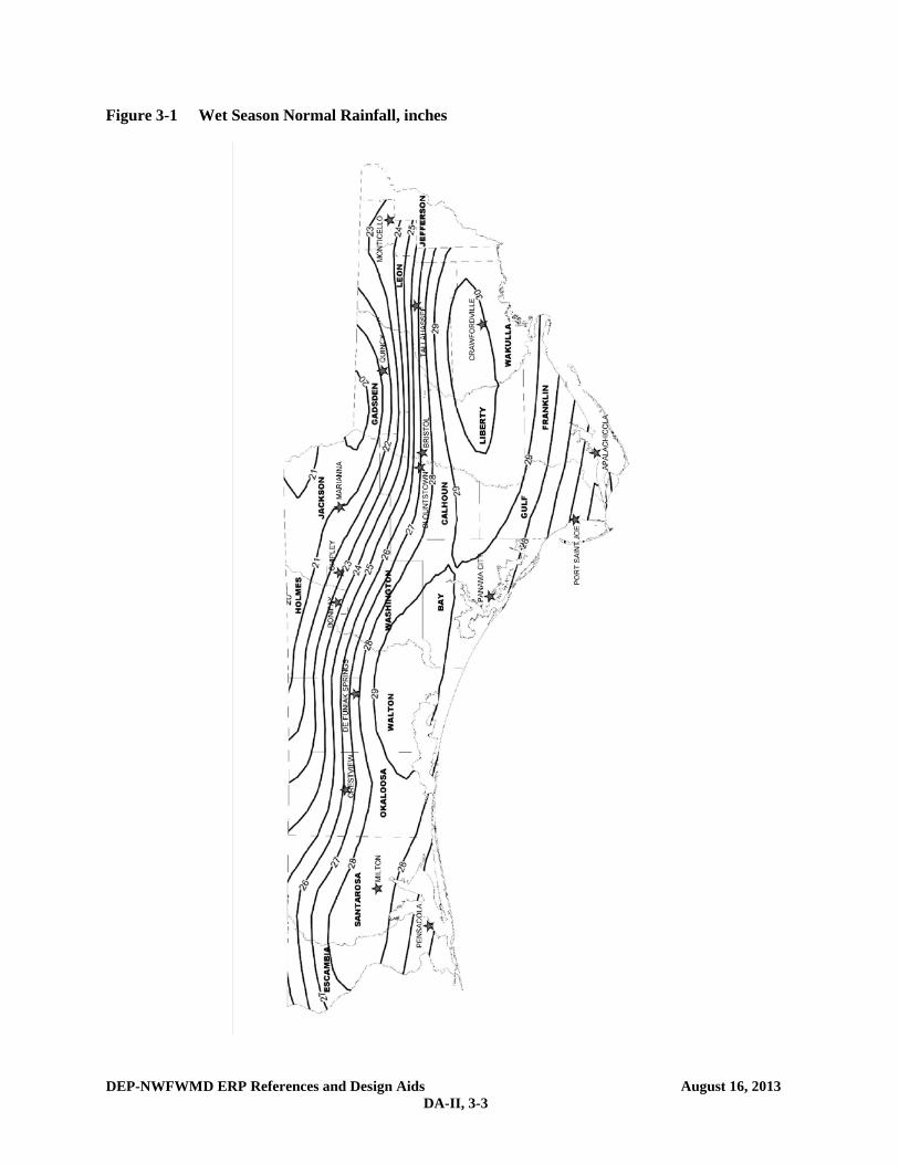
The depth of the wet season rainfall (R) for areas of the NWFWMD is shown in Figure 3-1, below. The rainfall depth at a particular location may be established by interpolating between the nearest isopluvial lines.
Substituting Equation 3-3 into Equation 3-2 gives:
PPV = DA C R RT
WS CF (3-4)
where: CF = Conversion factor = 12 in/ft
3.2 Sizing the Drawdown Structure
The rule requires that no more than half the treatment volume should be discharged in the first 48 to 60 hours after the storm event. A popular means of meeting this requirement is to use an orifice or a weir. The following subsections show procedures for sizing an orifice and V-notch weir to meet the drawdown requirements.

DEP-NWFWMD ERP References and Design Aids August 16, 2013 DA-II, 3-2
Table 3-1 Selected Runoff Coefficients (C) for a Design Storm Return Period of Ten Years or Less1
Sandy Soils Clay Soils
Slope Land Use Min. Max. Min. Max. Flat (0-2%) Lawns 0.05 0.10 0.13 0.17 Rooftops and pavement 0.95 0.95 0.95 0.95 Woodlands 0.10 0.15 0.15 0.20 Pasture, grass, and farmland2 0.15 0.20 0.20 0.25 Rolling (2-7%) Lawns 0.10 0.15 0.18 0.22 Rooftops and pavements 0.95 0.95 0.95 0.95 Woodlands 0.15 0.20 0.20 0.25 Pasture, grass, and farmland2 0.20 0.25 0.25 0.30 Steep (>7%) Lawns 0.15 0.20 0.25 0.35 Rooftops and pavements 0.95 0.95 0.95 0.95 Woodlands 0.20 0.25 0.25 0.30 Pasture, grass, and farmland2 0.25 0.35 0.30 0.40
1For 25- to 100-yr recurrence intervals, multiply coefficient by 1.1 and 1.25, respectively, and the product cannot exceed
1.0. 2 Depends on depth and degree of permeability of underlying strata.
DEP-NWFWMD ERP References and Design Aids August 16, 2013 DA-II, 3-3
Figure 3-1 Wet Season Normal Rainfall, inches
DEP-NWFWMD ERP References and Design Aids August 16, 2013 DA-II, 3-4
3.2.1 Sizing an Orifice
The orifice equation is given by: Q = C A 2 g h (3-5)
where: Q = Rate of discharge (cfs) A = Orifice area (ft2) G = Gravitational constant = (32.2 ft/sec2) H = Depth of water above the flow line (center) of the orifice (ft) C = Orifice coefficient (usually assumed = 0.6)
The average discharge rate (Q) required to drawdown half the treatment volume (TV) in a desired amount of time (t) is:
Q = TV
2 t CF (3-6)
where: TV = Treatment Volume (ft3) t = Recovery time (hrs) CF = Conversion Factor = 3600 sec/hr
The depth of water (h) should be set to the average depth above the flow line between the top of the treatment volume and the stage at which half the treatment volume has been released:
h = ( 1h + 2h )
2 (3-7)
where: h1 = Depth of water between the top of the treatment volume and the flow line (ft) h2 = Depth of water between the stage when half the treatment volume has been
released and the flow line of the orifice (ft)
Equation 3-5 can be rearranged to solve for the area (A):
A = Q
C 2 g h (3-8)
The diameter (D) of an orifice is calculated by:
D =
4 Aπ (3-9)
where: D = Diameter of the orifice (ft)

DEP-NWFWMD ERP References and Design Aids August 16, 2013 DA-II, 3-5
3.2.2 Sizing a V-notch Weir
Discharge (Q) through a V-notch opening in a weir can be estimated by:
Q = 2.5 tanθ2
2.5h (3-10)
where: Q = Discharge (cfs)
θ = Angle of V-notch (degrees) h = Head on vertex of notch (ft)
The average discharge rate (Q) required to draw down half the treatment volume (TV) in a desired amount of time (t) is:
Q =
TV2 t CF (3-11)
where: TV = Treatment Volume (ft3)
t = Recovery time (hrs) CF = Conversion Factor = 3600 sec/hr
The depth of water (h) should be set to the average depth above the vertex of the notch between the top of the treatment volume and the stage at which half the treatment volume has been released:
h = (h + h )
21 2
(3-12)
where: h1 = Depth of water between the top of the treatment volume and the vertex of the notch (ft)
h2 = Depth of water between the stage when half the treatment volume has been released and the vertex of the notch (ft)
Equation 3-10 can be rearranged to solve for the V-notch angle (θ):
h 2.5Q 2 = 2.5
1-tanθ (3-13)
Substituting Equation 3-11 into Equation 3-13 and simplifying gives:
θ = 2 -1tan
TV5 t CF 2.5h
(3-14)
DEP-NWFWMD ERP References and Design Aids August 16, 2013 DA-II, 3-6
3.3 Mean Depth of the Pond
The mean depth (MD) of a pond can be calculated from:
MD =
PPVPA (3-15)
where: MD = Mean depth of the pond (ft) AP = Area of pond measured at the control elevation (ft2)
3.4 Design Example
Given: Residential development in Crawfordville, Wakulla County Class III receiving waters Project area = 100 acres; Project runoff coefficient = 0.35 Project percent impervious (not including pond area) = 30% Off-site drainage area = 10 acres; Off-site percent impervious = 0% Off-site runoff coefficient = 0.2 Average on-site groundwater table elevation at the proposed lake = 20.0 ft Design tailwater elevation = 19.5 ft Pond area at elevation 20.0 ft = 5.0 acres No planted littoral zone proposed, 50% additional permanent pool required The proposed wet detention lake has the following stage-storage relationship:
Stage (ft)
Storage (ac-ft)
9.0 0.0 20.0 18.0 25.0 35.5
Design Calculations: Step 1. Calculate the required treatment volume. The agency requires a treatment volume of 1 inch of runoff.
Treatment volume required = (110 ac.)(1 inch) = 9.17 ac-ft
(one inch of runoff) 12 in/ft Treatment volume = 9.17 ac-ft
Step 2. Set the elevation of the control structure. Set the orifice invert at or above the seasonal high water table and design tailwater elevation. Therefore, set the orifice invert elevation at 20.0 ft.
DEP-NWFWMD ERP References and Design Aids August 16, 2013 DA-II, 3-7
Set an overflow weir at the top of the treatment volume storage to discharge runoff volumes greater than the treatment volume. Utilizing the stage-area-storage relationship, interpolate between 20.0 and 25.0 ft.
( ) ft62.22ft20)ftac0.18()ftac5.35(
ftac17.9ft20ft25. =+−−−
−×−=elevWeir
Step 3. Calculate the minimum permanent pool volume that will provide the required residence time. The permanent pool must be sized to provide a residence time of at least 21 days (14 days plus 50% additional) during the wet season (June - September), to account for the design with no planted littoral zone. The length of the wet season (WS) = 122 days From Figure 3-1, the wet season rainfall depth (R) for Crawfordville = 30 inches The minimum residence time (RT) = 21 days The runoff coefficient (C) for the drainage area to the wet detention pond is:
( )( ) ( )( ) 37.0
ac1102.0ac10)0.1)(ac0.5(35.05.0ac-ac100
=++
=C
Utilizing Equation 3-4:
( )( )( )( )
( ) ftac5.17in/ft12days122
days21in3037.0ac110−==volumepoolPermanent
The pond volume below elevation 20.0 feet is 18.0 ac-ft. Therefore, adequate storage is provided to satisfy the permanent pool criteria. Step 4. Size a circular orifice to recover one-half the treatment volume in 48 hours. Since the size of the orifice has yet to be determined, use the invert elevation of the orifice as an approximation of the flow line (center) of the orifice. After calculating the orifice size, adjust the flow line elevation and calculate the orifice size again.
Treatment volume depth (h1) = 22.62 ft - 20.00 ft = 2.62 ft
( ) ( ) ft31.21ft20.0ft20.0ft25.0ftac(18.0ft)ac5.35
5.0ft)ac9.17(=+−×
−−−×−
=volumetreatmentthehalfatStage
ft1.31ft20.00ft21.312 =−=h
From Equation 3-7:
( ) ft97.1
2ft1.31ft2.62
=+
=h
DEP-NWFWMD ERP References and Design Aids August 16, 2013 DA-II, 3-8
The average flow rate (Q) required to drawdown one-half the treatment volume is found from Equation 3-6:
cfs16.1sec3600
1hrs481
2/acft43560ftac17.9 2
=×××−
=Q
Find the area (A) of the orifice utilizing Equation 3-8:
Given: C = 0.6 G = 32.2 ft/sec2
ft 0.172ft 1.97 )secft/ (32.2 2 0.6
/secft 1.16 22
3
= = A
From Equation 3-9, the orifice diameter (D) is:
inches 5.6f 0.468 3.1416
)ft (0.172 4 2
= t = = D
For a vertical orifice, adjust h1, h2, and the orifice diameter (D) to the flow line of the orifice.
ft20.232
ft0.468ft.0020 =+=elevationlineFlow
th f2.39ft20.23ft22.621 =−=
th f1.08ft20.23ft31.212 =−=
ft1.742
ft1.08ft2.39=
+=h
ft 0.183ft 1.74 )secft/ (32.2 2 0.6
/secft 1.16 22
3
= = A
inches 5.8ft 0.4833.1416
)ft (0.183 4 2
= = = D
ft20.242
ft0.483ft00.20. =+=elevlineFlow
20.24 ft vs 20.23 ft = 0.01 ft difference which is acceptable
Step 5. Check the mean depth of the pond. The mean depth of the permanent pool must be between 2 and 8 feet. From Equation 3-15:
DEP-NWFWMD ERP References and Design Aids August 16, 2013 DA-II, 3-9
mean depth = 17.5 ac-ft = 3.5 ft which is consistent with the mean depth criteria. 5.0 ac
Additional Steps. In a typical design, the applicant would have to design the following:
(a) Pond shape to provide at least 2:1 length to width ratio (b) Alignment of inlets and outlets to promote mixing and maximize flow path (c) Overflow weir to safely pass the design storm event(s) at pre-development peak discharge
rates. 3.5 Littoral Zone Planting Suggestions
The littoral zone is that portion of a wet detention pond which is designed to contain rooted aquatic plants. The littoral area is usually provided by extending and gently sloping the sides of the pond down to a depth of 2 to 3 feet below the normal water level or control elevation. Also, the littoral zone can be provided in other areas of the pond that have suitable depths (i.e., a shallow shelf in the middle of the lake).
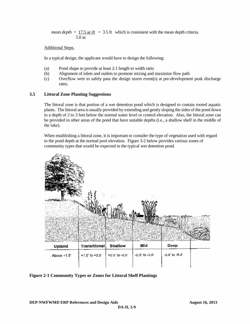
When establishing a littoral zone, it is important to consider the type of vegetation used with regard to the pond depth at the normal pool elevation. Figure 3-2 below provides various zones of community types that would be expected in the typical wet detention pond.
Figure 2-1 Community Types or Zones for Littoral Shelf Plantings
DEP-NWFWMD ERP References and Design Aids August 16, 2013 DA-II, 3-10
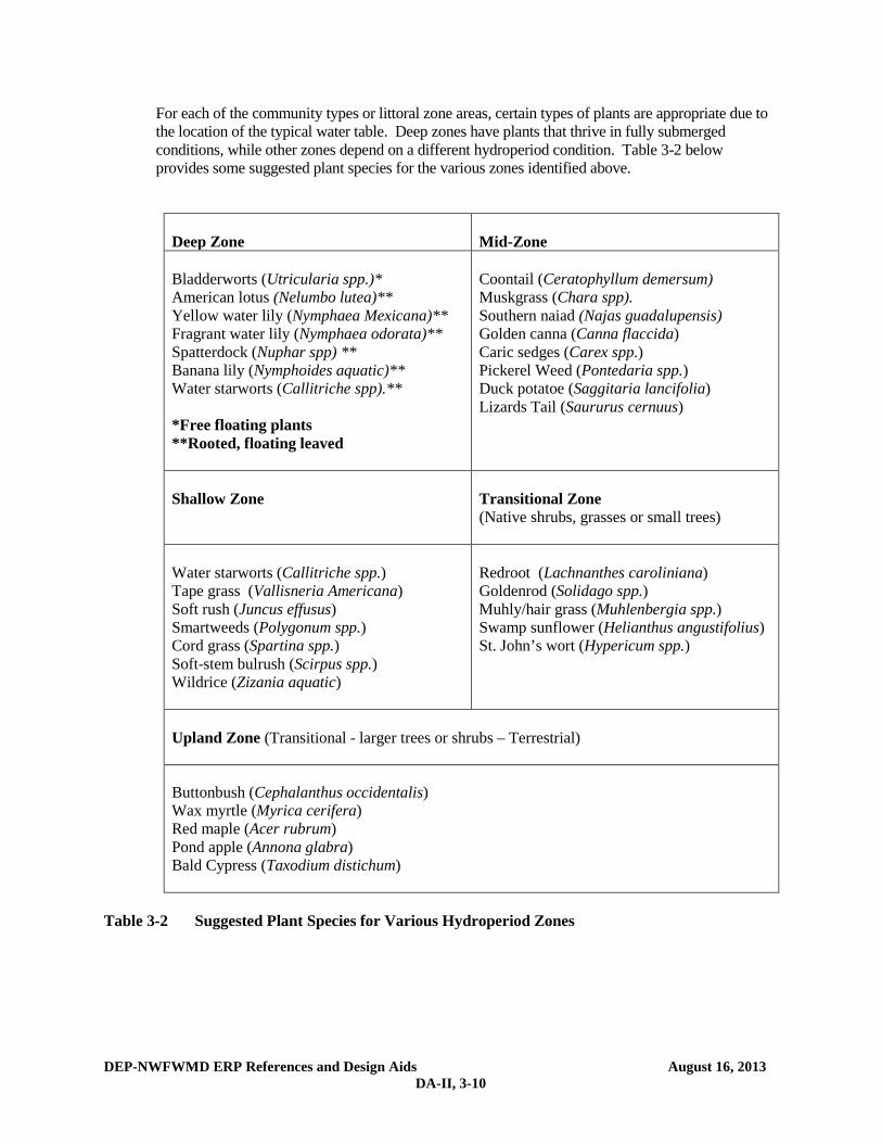
For each of the community types or littoral zone areas, certain types of plants are appropriate due to the location of the typical water table. Deep zones have plants that thrive in fully submerged conditions, while other zones depend on a different hydroperiod condition. Table 3-2 below provides some suggested plant species for the various zones identified above.
Deep Zone
Mid-Zone
Bladderworts (Utricularia spp.)* American lotus (Nelumbo lutea)** Yellow water lily (Nymphaea Mexicana)** Fragrant water lily (Nymphaea odorata)** Spatterdock (Nuphar spp) ** Banana lily (Nymphoides aquatic)** Water starworts (Callitriche spp).** *Free floating plants **Rooted, floating leaved
Coontail (Ceratophyllum demersum) Muskgrass (Chara spp). Southern naiad (Najas guadalupensis) Golden canna (Canna flaccida) Caric sedges (Carex spp.) Pickerel Weed (Pontedaria spp.) Duck potatoe (Saggitaria lancifolia) Lizards Tail (Saururus cernuus)
Shallow Zone
Transitional Zone (Native shrubs, grasses or small trees)
Water starworts (Callitriche spp.) Tape grass (Vallisneria Americana) Soft rush (Juncus effusus) Smartweeds (Polygonum spp.) Cord grass (Spartina spp.) Soft-stem bulrush (Scirpus spp.) Wildrice (Zizania aquatic)
Redroot (Lachnanthes caroliniana) Goldenrod (Solidago spp.) Muhly/hair grass (Muhlenbergia spp.) Swamp sunflower (Helianthus angustifolius) St. John’s wort (Hypericum spp.)
Upland Zone (Transitional - larger trees or shrubs – Terrestrial)
Buttonbush (Cephalanthus occidentalis) Wax myrtle (Myrica cerifera) Red maple (Acer rubrum) Pond apple (Annona glabra) Bald Cypress (Taxodium distichum)
Table 3-2 Suggested Plant Species for Various Hydroperiod Zones
DEP-NWFWMD ERP References and Design Aids August 16, 2013 DA-II, 4-1
4.0 Methodology and Design Example for Swales Infiltration from swale systems follows the same processes discussed in section 1.1 for retention
systems. However, unlike retention systems, swales are an "open" conveyance facility which must infiltrate a specified portion of runoff from the three-year, one-hour storm without the aid of berms, check dams, etc. Also, the swale must be sized to convey a design storm without being subjected to erosive velocities. The following methodology, which is adapted from Livingston et al. (1988), is recommended for designing swales to percolate the desired portion of runoff and to convey the design flow rate with acceptable velocities.
4.1 Runoff Hydrograph and Volume The rational method can be utilized to estimate peak runoff rates for small urban areas. The traditional
rational formula is expressed as: Q = C I A (4-1) where: Q = Peak runoff rate (cfs) C = Runoff coefficient I = Rainfall intensity (in./hr) A = Drainage area (acres) Values for the runoff coefficient (C) are contained in Table 3-1 in Section 3.2. The intensity (I) is
determined from intensity-duration-frequency (IDF) curves such as those published by the Florida Department of Transportation (1987).
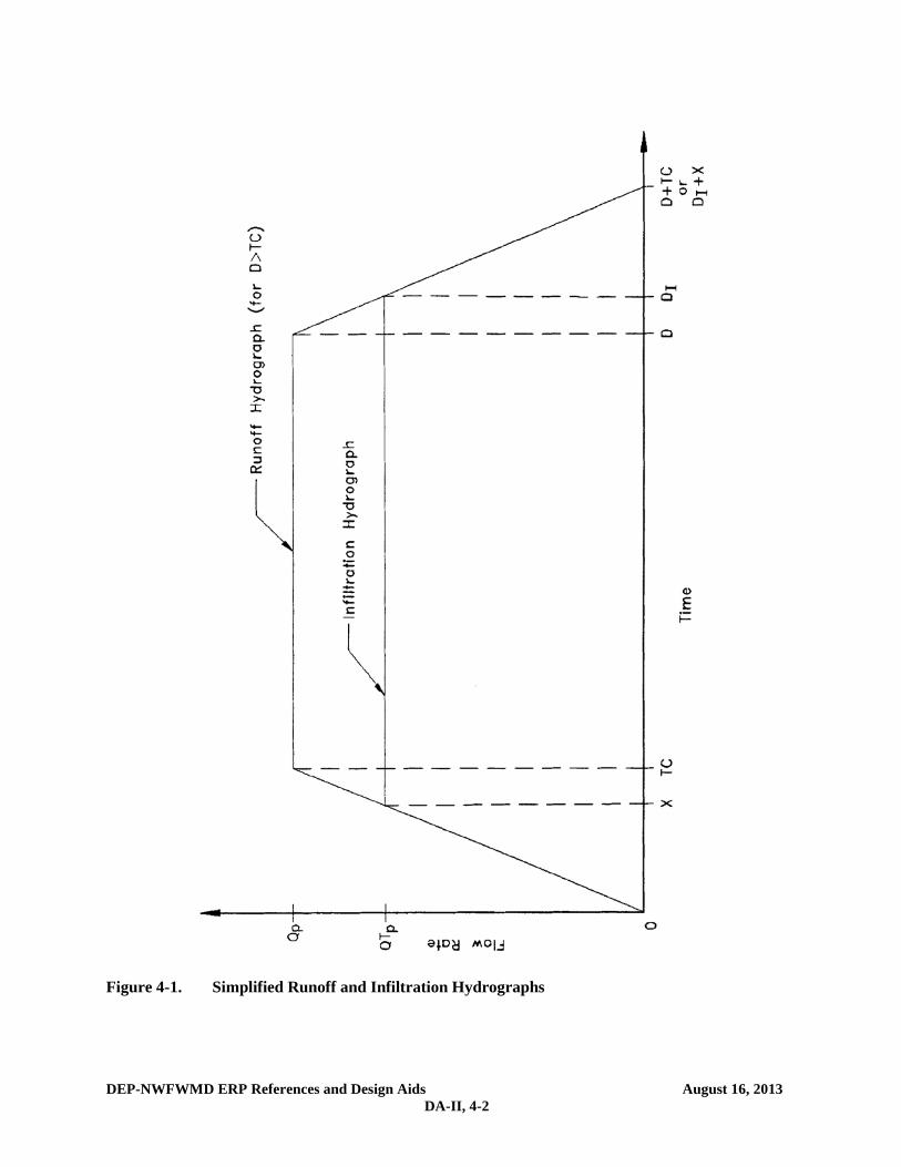
A simplified runoff hydrograph for a specific design storm with given duration (D) can be constructed
given the time of concentration (Tc) of the drainage area. As seen in Figure 4-1, this modified simplified runoff hydrograph is a modification of the traditional rational formula. The implied assumption behind Figure 4-1 is that the drainage basin time of concentration (Tc) is less than the duration (D) of the design storm event.
The peak runoff rate from this simplified hydrograph method is not the "traditional" rational peak
discharge rate at the basin time of concentration but a sustained and lower peak runoff rate (QP) resulting from the rainfall intensity as determined for the desired duration of the storm. The sustained peak runoff rate is expressed as:
QP = C ID A (4-2) where: QP = Peak runoff rate from the 3-year, 1-hour rainfall intensity (cfs) ID = Average rainfall intensity for a one hour duration (in./hr)
DEP-NWFWMD ERP References and Design Aids August 16, 2013 DA-II, 4-2
Figure 4-1. Simplified Runoff and Infiltration Hydrographs
DEP-NWFWMD ERP References and Design Aids August 16, 2013 DA-II, 4-3
The volume of runoff (VR) is equal to the area under the runoff hydrograph curve in Figure 4-1 and can be expressed as:
RV = 12
PQ Tc + PQ (D - Tc) + 12
PQ (D + Tc - D) (4-3)
which can be simplified to: RV = PQ D (4-4) where: VR = Volume of runoff (ft3) Tc = Time of concentration (hr) D = Rainfall duration (hr) 4.2 Infiltration Hydrograph and Volume The peak infiltration rate and volume should be calculated using one of the acceptable methodologies listed in section 1.3 for vertical unsaturated infiltration. Utilizing the modified Green and Ampt Equation the peak infiltration rate is the design infiltration rate (Id) and is expressed as:
dI = vuKFS
(4-5)
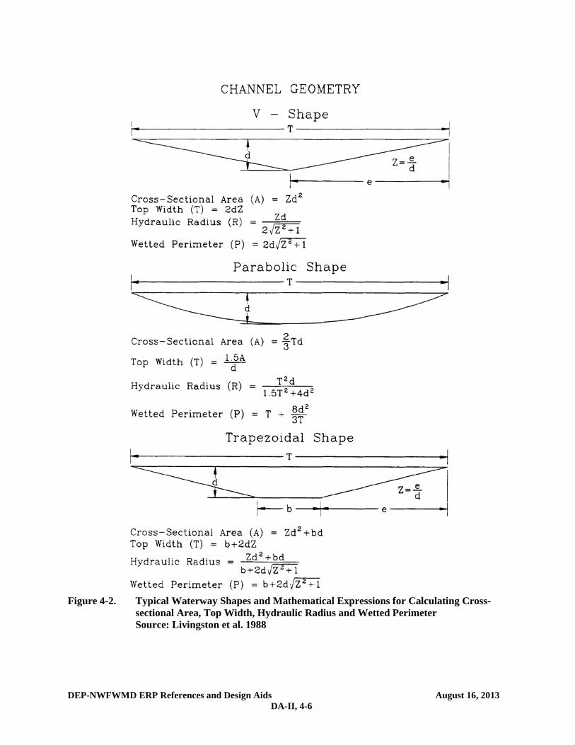
where: Id = Design infiltration rate (ft/hr) Kvu = Unsaturated vertical hydraulic conductivity (ft/hr) FS = Factor of safety (recommend FS = 2.0) The area of swale bottom and side slopes (Ab) in which infiltration will occur is: bA = L P (4-6) where: Ab = Area of swale bottom and side slopes in which infiltration will occur (ft2) L = Length of swale (ft) P = Wetted perimeter (ft) The peak infiltration flow rate (QiP) is: PQi = dI bA = dI L P (4-7) where: QiP = Peak infiltration flow rate (ft3/hr) The wetted perimeter (P) is dependent on the geometry of the swale. Equations for the wetted perimeter for three common swale shapes are given in Figure 4-2. A simple infiltration hydrograph can be constructed as in Figure 4-1. The volume infiltrated is the area under the infiltration hydrograph curve and can be expressed as:
IV = 12
PQi X + PQi ( ID - X) + 12
PQi ( ID + X - ID ) (4-8)
DEP-NWFWMD ERP References and Design Aids August 16, 2013 DA-II, 4-4
and simplified to: IV = PQi ID (4-9) where: VI = Volume of runoff infiltrated (ft3) DI = Time from the beginning of the storm to the end of the peak infiltration flow rate (hr) X = Time from DI to the end of the runoff hydrograph (hr) Based on Figure 4-1, DI can be expressed as: DI = D + Tc - X (4-10) and X can be expressed as:
X = Tc PQi
PQ (4-11)
Substituting equations 4-10 and 4-11 into 4-9 gives:
IV = PQi D + Tc - Tc PQi
PQ
(4-12)
If the volume infiltrated (VI) is greater than or equal to the required portion (i.e., 80%) of the runoff volume (VR) then the design is adequate for treatment purposes. In addition, the design should be checked to ensure that the swale can convey the design storm runoff without reaching erosive velocities. 4.3 Velocity
The velocity of flow in an open channel can be found from Manning's Equation:
V = 1.49
n 2/3R 1/2S (4-13)
DEP-NWFWMD ERP References and Design Aids August 16, 2013 DA-II, 4-5
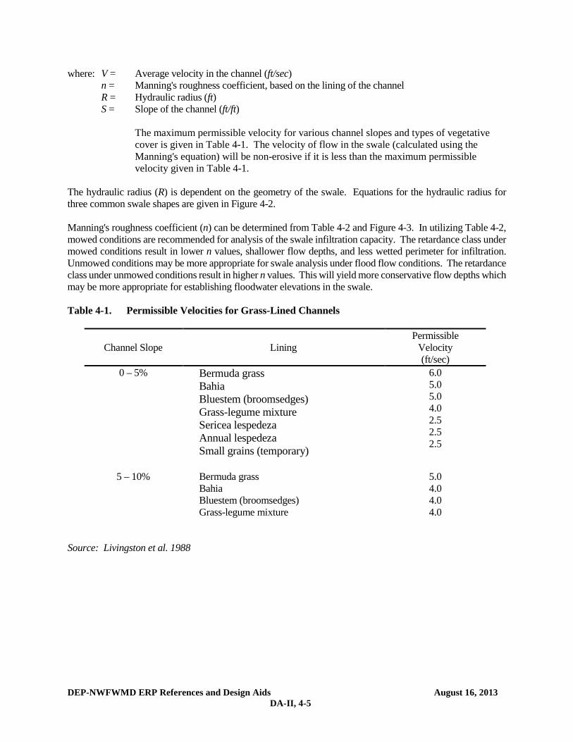
where: V = Average velocity in the channel (ft/sec) n = Manning's roughness coefficient, based on the lining of the channel R = Hydraulic radius (ft) S = Slope of the channel (ft/ft)
The maximum permissible velocity for various channel slopes and types of vegetative cover is given in Table 4-1. The velocity of flow in the swale (calculated using the Manning's equation) will be non-erosive if it is less than the maximum permissible velocity given in Table 4-1.
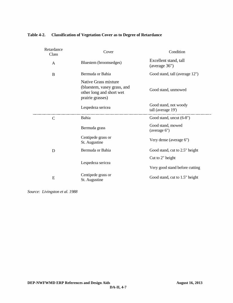
The hydraulic radius (R) is dependent on the geometry of the swale. Equations for the hydraulic radius for three common swale shapes are given in Figure 4-2. Manning's roughness coefficient (n) can be determined from Table 4-2 and Figure 4-3. In utilizing Table 4-2, mowed conditions are recommended for analysis of the swale infiltration capacity. The retardance class under mowed conditions result in lower n values, shallower flow depths, and less wetted perimeter for infiltration. Unmowed conditions may be more appropriate for swale analysis under flood flow conditions. The retardance class under unmowed conditions result in higher n values. This will yield more conservative flow depths which may be more appropriate for establishing floodwater elevations in the swale. Table 4-1. Permissible Velocities for Grass-Lined Channels
Channel Slope Lining Permissible
Velocity (ft/sec)
0 – 5% Bermuda grass Bahia Bluestem (broomsedges) Grass-legume mixture Sericea lespedeza Annual lespedeza Small grains (temporary)
6.0 5.0 5.0 4.0 2.5 2.5 2.5
5 – 10% Bermuda grass Bahia Bluestem (broomsedges) Grass-legume mixture
5.0 4.0 4.0 4.0
Source: Livingston et al. 1988
DEP-NWFWMD ERP References and Design Aids August 16, 2013 DA-II, 4-6
Figure 4-2. Typical Waterway Shapes and Mathematical Expressions for Calculating Cross-
sectional Area, Top Width, Hydraulic Radius and Wetted Perimeter Source: Livingston et al. 1988
DEP-NWFWMD ERP References and Design Aids August 16, 2013 DA-II, 4-7
Table 4-2. Classification of Vegetation Cover as to Degree of Retardance
Retardance Class Cover Condition
A Bluestem (broomsedges) Excellent stand, tall (average 36")
B Bermuda or Bahia Good stand, tall (average 12")
Native Grass mixture (bluestem, vasey grass, and other long and short wet prairie grasses)
Good stand, unmowed
Lespedeza sericea Good stand, not woody tall (average 19')
C Bahia Good stand, uncut (6-8")
Bermuda grass Good stand, mowed (average 6")
Centipede grass or St. Augustine Very dense (average 6")
D Bermuda or Bahia Good stand, cut to 2.5" height
Lespedeza sericea Cut to 2" height Very good stand before cutting
E Centipede grass or St. Augustine Good stand, cut to 1.5" height
Source: Livingston et al. 1988

DEP-NWFWMD ERP References and Design Aids August 16, 2013 DA-II, 4-8
Figure 4-3. Manning's "n" Related to Velocity, Hydraulic Radius and Vegetal Retardance Source: Livingston et al. 1988
DEP-NWFWMD ERP References and Design Aids August 16, 2013 DA-II, 4-9
4.4 Capacity Manning's Equation (Equation 4-13) and the Continuity Equation (Q = V A) can be combined to determine flow capacity of an open channel:
Q = 1.49
n 2/3R 1/2S A (4-14)
where: Q = Flow in the channel (ft3/sec) A = Cross-section area of the channel (ft2) The cross-sectional area (A) is dependent on the channel shape and equations for the cross-sectional area for three common swale shapes are given in Figure 4-2. In addition to the treatment capacity of the swale, the design of the swale must be adequate to provide flood protection in accordance with the requirements of local agencies. 4.5 Vertical Unsaturated and Lateral Saturated Infiltration The design of the swale system should be checked using one of the accepted methodologies in section 26 to insure that lateral saturated infiltration does not occur. Lateral saturated infiltration occurs when the ground water table "mounds" beneath the swale and intercepts the swale bottom. See section 26 for a complete description of infiltration processes. Utilizing the methodology described in section 1.3.3, the volume infiltrated under vertical unsaturated flow (Vu) is determined from the following equation:
bbu fhAV = where: Vu = Volume of water required to saturate the soil below the swale hb = Height of swale bottom above the ground water table f = Fillable porosity (generally 0.2 to 0.3) If Vu > VR infiltration will occur entirely under vertical unsaturated flow conditions. 4.6 Example Design Calculations for Swale Systems Given: Residential project in Palatka discharging to Class III waters Drainage area = 10 acres Post-development runoff coefficient = 0.4 Tc = 20 minutes; S = 3% f = 0.3; Kvs = 36 in/hr; FS = 2.0; hb = 10 ft Rectangular project site with dimensions of length = 660 ft and width = 660 ft Three streets each 600 ft long with swales on both sides
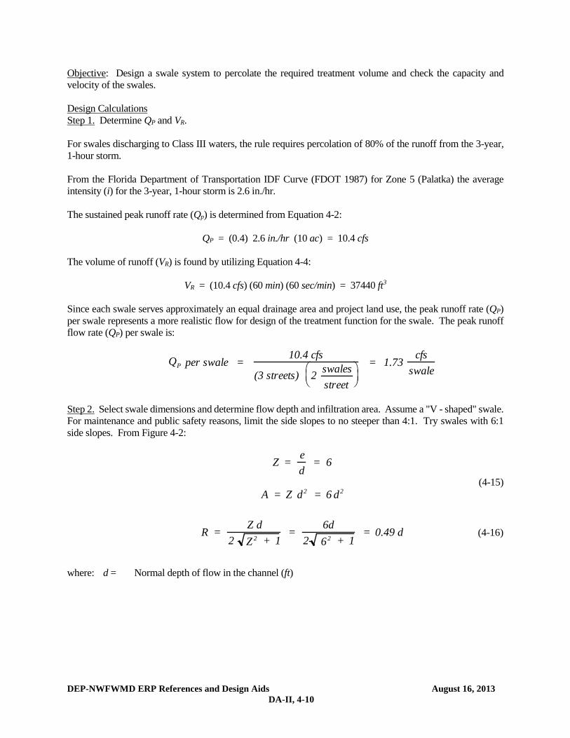
DEP-NWFWMD ERP References and Design Aids August 16, 2013 DA-II, 4-10
Objective: Design a swale system to percolate the required treatment volume and check the capacity and velocity of the swales. Design Calculations Step 1. Determine QP and VR. For swales discharging to Class III waters, the rule requires percolation of 80% of the runoff from the 3-year, 1-hour storm. From the Florida Department of Transportation IDF Curve (FDOT 1987) for Zone 5 (Palatka) the average intensity (i) for the 3-year, 1-hour storm is 2.6 in./hr. The sustained peak runoff rate (Qp) is determined from Equation 4-2:
QP = (0.4) 2.6 in./hr (10 ac) = 10.4 cfs The volume of runoff (VR) is found by utilizing Equation 4-4:
VR = (10.4 cfs) (60 min) (60 sec/min) = 37440 ft3 Since each swale serves approximately an equal drainage area and project land use, the peak runoff rate (QP) per swale represents a more realistic flow for design of the treatment function for the swale. The peak runoff flow rate (QP) per swale is:
PQ per swale = 10.4 cfs
(3 streets) 2 swalesstreet
= 1.73 cfs
swale
Step 2. Select swale dimensions and determine flow depth and infiltration area. Assume a "V - shaped" swale. For maintenance and public safety reasons, limit the side slopes to no steeper than 4:1. Try swales with 6:1 side slopes. From Figure 4-2:
Z = ed
= 6
(4-15) A = Z 2d = 6 2d
R = Z d
2 2Z + 1 =
6d2 26 + 1
= 0.49 d (4-16)
where: d = Normal depth of flow in the channel (ft)
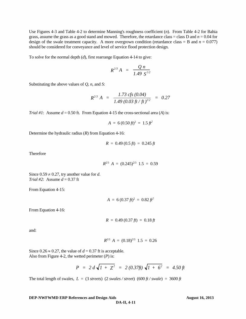
DEP-NWFWMD ERP References and Design Aids August 16, 2013 DA-II, 4-11
Use Figures 4-3 and Table 4-2 to determine Manning's roughness coefficient (n). From Table 4-2 for Bahia grass, assume the grass as a good stand and mowed. Therefore, the retardance class = class D and n = 0.04 for design of the swale treatment capacity. A more overgrown condition (retardance class = B and n = 0.077) should be considered for conveyance and level of service flood protection design. To solve for the normal depth (d), first rearrange Equation 4-14 to give:
2/3R A = Q n
1.49 1/2S
Substituting the above values of Q, n, and S:
2/31/2R A = 1.73 cfs (0.04)
1.49 (0.03 ft / ft ) = 0.27
Trial #1: Assume d = 0.50 ft. From Equation 4-15 the cross-sectional area (A) is: A = 6 (0.50 ft)2 = 1.5 ft2 Determine the hydraulic radius (R) from Equation 4-16: R = 0.49 (0.5 ft) = 0.245 ft Therefore R2/3 A = (0.245)2/3 1.5 = 0.59 Since 0.59 ≠ 0.27, try another value for d. Trial #2: Assume d = 0.37 ft From Equation 4-15: A = 6 (0.37 ft)2 = 0.82 ft2 From Equation 4-16: R = 0.49 (0.37 ft) = 0.18 ft and: R2/3 A = (0.18)2/3 1.5 = 0.26 Since 0.26 ≈ 0.27, the value of d = 0.37 ft is acceptable. Also from Figure 4-2, the wetted perimeter (P) is: P = 2 d 1 + 2Z = 2 (0.37ft) 1 + 26 = 4.50 ft The total length of swales, L = (3 streets) (2 swales / street) (600 ft / swale) = 3600 ft

DEP-NWFWMD ERP References and Design Aids August 16, 2013 DA-II, 4-12
From Equation 4-6, the total infiltration area (Ab) can be determined: Ab = L P = (3600 ft) 4.5 ft = 16200 ft2 The infiltration area (Ab) per swale is: Ab per swale = (600 ft) 4.5 ft = 2700 ft2 per swale Step 3. Check for lateral saturated infiltration (see section 26 for a complete description of infiltration processes). Volume infiltrated under vertical unsaturated flow (Vu) is determined from equation: Vu = Ab f hb = 16200 ft2 (0.3) 10 ft = 48600 ft3 Since Vu > VR infiltration will occur entirely under vertical unsaturated flow conditions. Therefore, analysis of lateral saturated infiltration will not be required for this example. Step 4. Calculate the peak infiltration flow rate (QiP). The unsaturated vertical hydraulic conductivity (Kvu) is found by equation:
( ) hrinhrinKvu /.24
3/.362
==
From Equation 4-5, the design infiltration rate (Id) is:
hrinhrinId /.122
/.24==
The peak infiltration rate (QiP) per swale is determined by Equation 4-7 with the infiltration area (Ab) per swale = 2700 ft2: QiP per swale = 12 in./hr (2700 ft2 per swale) (1 ft / 12 in.) (1 hr / 60 min) QiP per swale = 45.0 ft3/min = 0.75 ft3/sec per swale
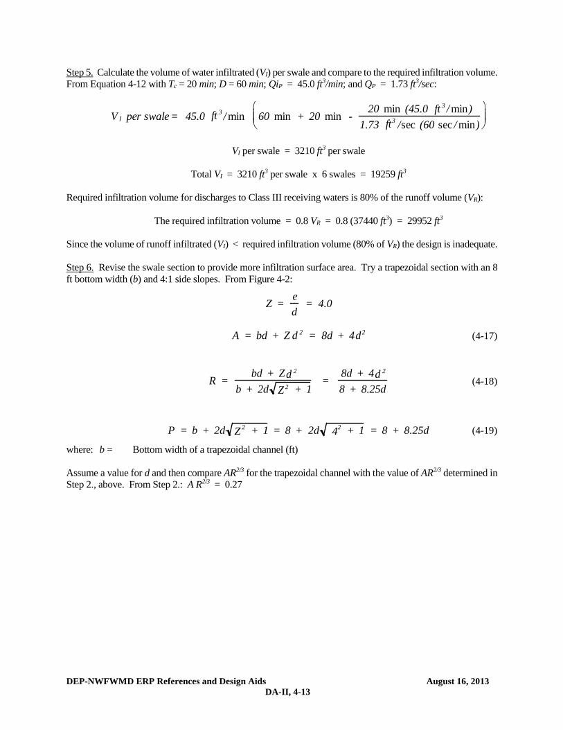
DEP-NWFWMD ERP References and Design Aids August 16, 2013 DA-II, 4-13
Step 5. Calculate the volume of water infiltrated (VI) per swale and compare to the required infiltration volume. From Equation 4-12 with Tc = 20 min; D = 60 min; QiP = 45.0 ft3/min; and QP = 1.73 ft3/sec:
IV per swale = 45.0 3ft / min 60 min + 20 min - 20 min (45.0 3ft / min)
1.73 3ft /sec (60 sec / min)
VI per swale = 3210 ft3 per swale Total VI = 3210 ft3 per swale x 6 swales = 19259 ft3 Required infiltration volume for discharges to Class III receiving waters is 80% of the runoff volume (VR): The required infiltration volume = 0.8 VR = 0.8 (37440 ft3) = 29952 ft3 Since the volume of runoff infiltrated (VI) < required infiltration volume (80% of VR) the design is inadequate. Step 6. Revise the swale section to provide more infiltration surface area. Try a trapezoidal section with an 8 ft bottom width (b) and 4:1 side slopes. From Figure 4-2:
Z = ed
= 4.0
A = bd + Z 2d = 8d + 4 2d (4-17)
R = bd + Z 2d
b + 2d 2Z + 1 =
8d + 4 2d8 + 8.25d
(4-18)
P = b + 2d 2Z + 1 = 8 + 2d 24 + 1 = 8 + 8.25d (4-19)
where: b = Bottom width of a trapezoidal channel (ft) Assume a value for d and then compare AR2/3 for the trapezoidal channel with the value of AR2/3 determined in Step 2., above. From Step 2.: A R2/3 = 0.27
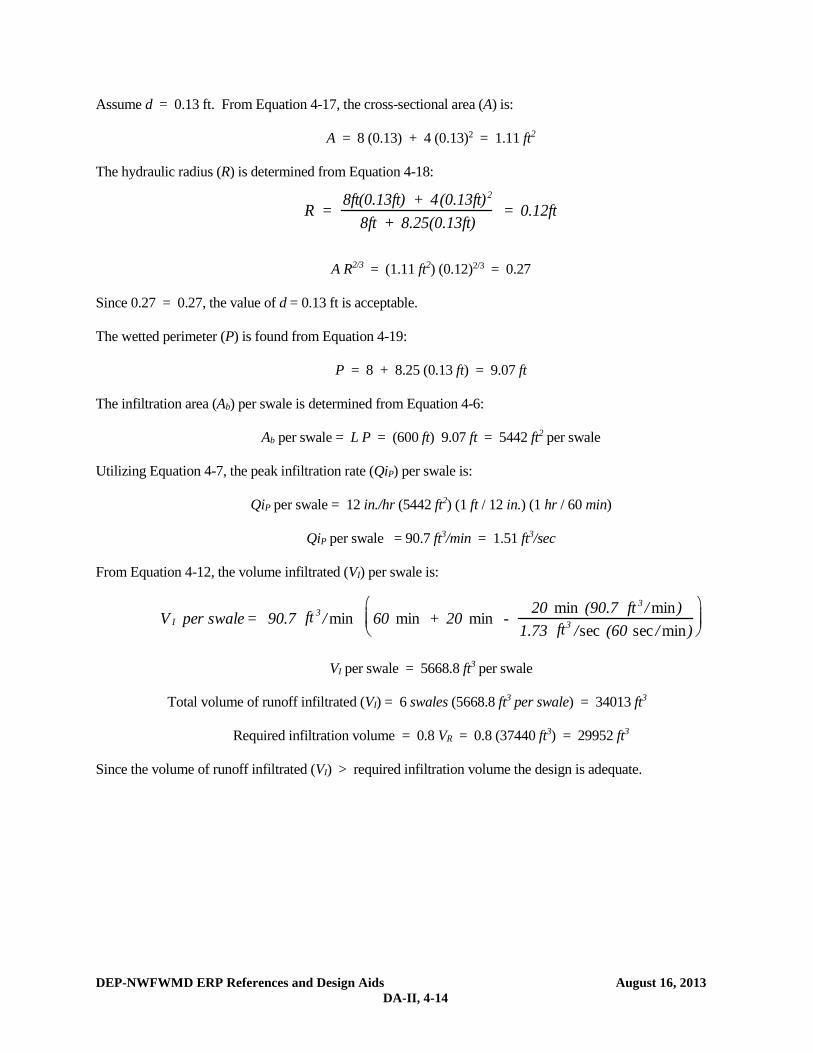
DEP-NWFWMD ERP References and Design Aids August 16, 2013 DA-II, 4-14
Assume d = 0.13 ft. From Equation 4-17, the cross-sectional area (A) is: A = 8 (0.13) + 4 (0.13)2 = 1.11 ft2 The hydraulic radius (R) is determined from Equation 4-18:
R = 8ft(0.13ft) + 4 2(0.13ft)
8ft + 8.25(0.13ft) = 0.12ft
A R2/3 = (1.11 ft2) (0.12)2/3 = 0.27 Since 0.27 = 0.27, the value of d = 0.13 ft is acceptable. The wetted perimeter (P) is found from Equation 4-19: P = 8 + 8.25 (0.13 ft) = 9.07 ft The infiltration area (Ab) per swale is determined from Equation 4-6: Ab per swale = L P = (600 ft) 9.07 ft = 5442 ft2 per swale Utilizing Equation 4-7, the peak infiltration rate (QiP) per swale is: QiP per swale = 12 in./hr (5442 ft2) (1 ft / 12 in.) (1 hr / 60 min) QiP per swale = 90.7 ft3/min = 1.51 ft3/sec From Equation 4-12, the volume infiltrated (VI) per swale is:
IV per swale = 90.7 3ft / min 60 min + 20 min - 20 min (90.7 3ft / min)
1.73 3ft /sec (60 sec / min)
VI per swale = 5668.8 ft3 per swale Total volume of runoff infiltrated (VI) = 6 swales (5668.8 ft3 per swale) = 34013 ft3 Required infiltration volume = 0.8 VR = 0.8 (37440 ft3) = 29952 ft3 Since the volume of runoff infiltrated (VI) > required infiltration volume the design is adequate.

DEP-NWFWMD ERP References and Design Aids August 16, 2013 DA-II, 4-15
Step 7. Calculate the velocity in the swale and compare with permissible values. From Table 4-1, for Bahia grass the maximum permissible velocity (Vmax) is 5.0 ft/sec. Calculate the velocity of the swales from Equation 4-13:
V = 1.490.04
2/3(0.12) (0.03 1/2) = 1.57 ft/ sec
The calculated velocity of flow in the swale (1.57 ft/sec) will be non-erosive since it is less than the maximum permissible velocity (5 ft/sec) given in Table 4-1.

DEP-NWFWMD ERP References and Design Aids August 16, 2013 DA-II, 5-1
5.0 Methodology and Design Examples for Stormwater Harvesting Systems 5.1 Overview
Water budgets are utilized to design stormwater harvesting systems. A water budget is an accounting of water movement onto, within, and off of an area. The purpose of developing a water budget for stormwater harvesting systems is to quantify the reduction in offsite discharge by harvesting for a given period of time. Individual components of water supply, storage, use, and movement must be accounted for in the water budget. Calculation of these components requires knowledge of the watershed characteristics, harvesting area (if irrigation is to be used), desired percentage of runoff to be harvested, harvesting volume, harvesting rate, rainfall data, and evaporation data. Using the above parameters, researchers at the University of Central Florida simulated the long term behavior of harvesting ponds over time for various locations in Florida. The results of the simulations are presented in Rate-Efficiency-Volume (REV) curves. The REV curves can be used to design stormwater harvesting systems to meet the performance criteria described in section 12 of the NWFWMD Volume II. Harvesting curves for selected regions are provided in section 5.5 below. Important assumptions that must be kept in mind when using the REV curves include:
(a) Net ground water movement into or out of the pond is assumed to be zero. (b) The harvesting rate is constant over time. (c) The mean annual evaporation from the pond equals the mean annual rainfall on the pond. (d) The results are long term averages based on historical rainfall records. The results will not
give an indication of conditions during a wet or dry year. To design a harvesting system which does not meet one of the above assumptions, the applicant can develop a site specific water budget analysis to meet the performance criteria described in section 12 of the NWFWMD Volume II. The following sections and example problems summarize the REV curve methodology for the design of stormwater harvesting systems.
5.2 Equivalent Impervious Area
When designing stormwater harvesting systems, the runoff characteristics of the watershed must be determined. The overall runoff coefficient (C) for an area composed of different surfaces can be determined by weighting the runoff coefficients for the surfaces with respect to the total areas they encompass:

DEP-NWFWMD ERP References and Design Aids August 16, 2013 DA-II, 5-2
C = 1C 1A + 2C 2A +. . . + NC NA1A + 2A + . . . + NA
(Equation 5-1)
where: CN = Runoff coefficient for surface N (see Table 3-1 for values of C) AN = Area of surface N
This weighted runoff coefficient (C) is termed the effective runoff coefficient and is representative of the entire watershed. The equivalent impervious area (EIA) is equal to the product of the total area of the watershed (A) and the effective, or weighted, runoff coefficient (C) for the watershed:
EIA = C A (Equation 5-2)
where: EIA = Equivalent impervious area (acres) C = Effective runoff coefficient for the watershed A = Area of watershed (acres)
The area of the EIA is defined as the area of a completely impervious watershed that would produce the same volume of runoff as the actual watershed. For example, a 20 acre watershed with an effective runoff coefficient (C) of 0.5 would have an EIA of 10 acres (20 ac x 0.5). If one inch of rain fell on this 10 acre impervious area, the runoff volume would be 10 ac-in (10 ac x 1 in). If the same amount of rain fell on the actual watershed the runoff volume would not change:
20 ac (1 in) (0.5) = 10 ac-in
The EIA will be expressed in acres throughout this methodology. The use of the EIA serves to generalize the model so that it can be applied to a watershed of any size and runoff characteristics. The EIA for a watershed should include the area of the pond when using this methodology.
5.3 Harvesting Volume
The harvesting volume (V) is the amount of runoff stored in the harvesting pond between the top of the permanent pool and the invert of the overflow structure (see Figure 12-1, of the NWFWMD Volume II). This volume is akin to the treatment volume in wet detention systems. The major difference between a harvesting pond and a wet detention pond is the operation of this storage volume. For wet detention systems, the treatment volume is designed to be discharged to adjacent surface waters via an overflow structure. On the other hand, in a harvesting pond the harvesting volume (V) is harvested and not discharged to adjacent surface waters. Harvesting volumes are expressed in units of inches over the EIA. The values can be converted to more practical units using simple conversions (see the example problems in section 5.7 below).
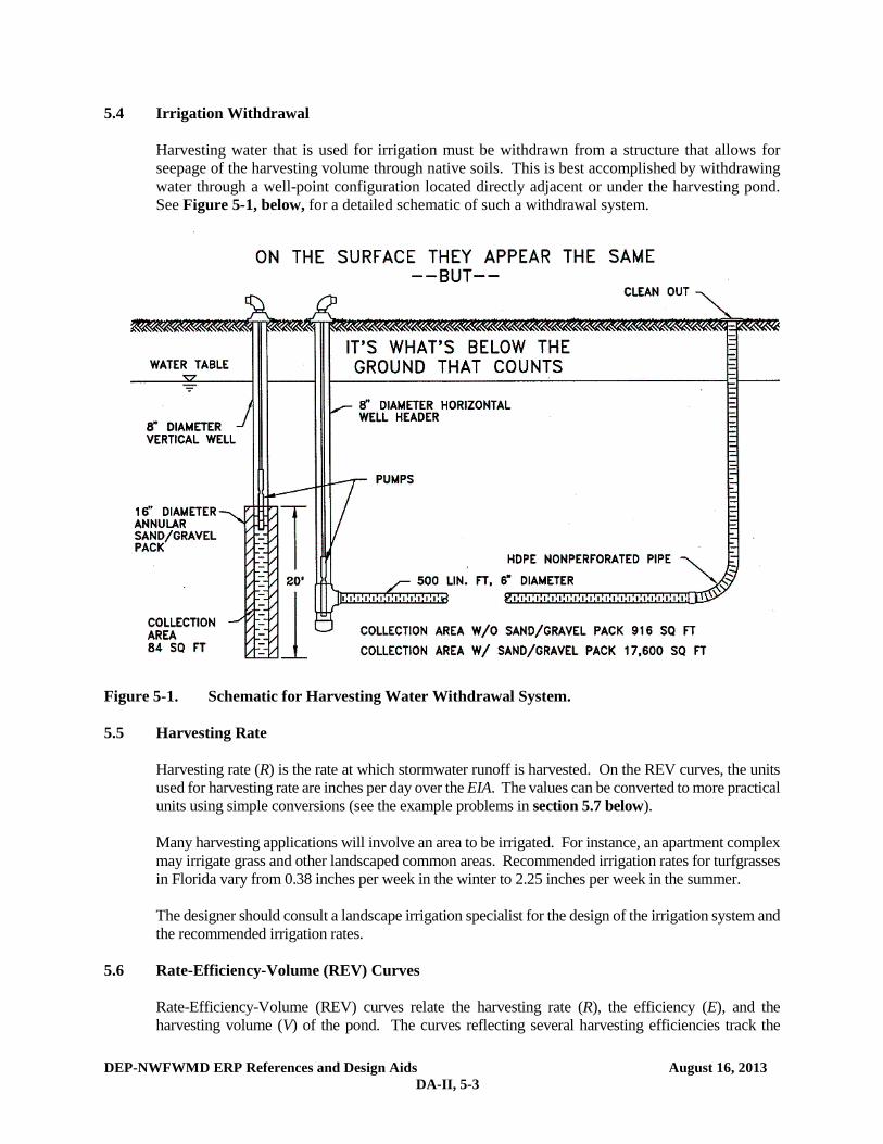
DEP-NWFWMD ERP References and Design Aids August 16, 2013 DA-II, 5-3
5.4 Irrigation Withdrawal
Harvesting water that is used for irrigation must be withdrawn from a structure that allows for seepage of the harvesting volume through native soils. This is best accomplished by withdrawing water through a well-point configuration located directly adjacent or under the harvesting pond. See Figure 5-1, below, for a detailed schematic of such a withdrawal system.
Figure 5-1. Schematic for Harvesting Water Withdrawal System.
5.5 Harvesting Rate
Harvesting rate (R) is the rate at which stormwater runoff is harvested. On the REV curves, the units used for harvesting rate are inches per day over the EIA. The values can be converted to more practical units using simple conversions (see the example problems in section 5.7 below). Many harvesting applications will involve an area to be irrigated. For instance, an apartment complex may irrigate grass and other landscaped common areas. Recommended irrigation rates for turfgrasses in Florida vary from 0.38 inches per week in the winter to 2.25 inches per week in the summer. The designer should consult a landscape irrigation specialist for the design of the irrigation system and the recommended irrigation rates.
5.6 Rate-Efficiency-Volume (REV) Curves
Rate-Efficiency-Volume (REV) curves relate the harvesting rate (R), the efficiency (E), and the harvesting volume (V) of the pond. The curves reflecting several harvesting efficiencies track the

DEP-NWFWMD ERP References and Design Aids August 16, 2013 DA-II, 5-4
appropriate combinations of harvesting rates and harvesting volumes. Information concerning any two of these three variables is necessary for the determination of the third. The REV curves are generalized for application to watersheds of any size or runoff coefficient via the EIA. The units of both the harvesting rate and harvesting volume are based on the EIA. Individual REV charts are specific to geographical regions with similar meteorological characteristics. The designer should use the one closest to the site for design. The REV charts for stations within the NWFWMD are presented in Table 5-1 and Figures 5-1 through 5-4, below. On every REV chart there is a curve for each of the following efficiency levels (in percentage): 50, 60, 70, 80, 90, and 95. The range of the curves is restricted by practical applicability. A harvesting rate of greater than 0.30 inches per day over the EIA would require such high quantities of supplement that the pond would act as no more than a large reservoir in the piping network of a groundwater irrigation system. Also, the storage required for volumes exceeding 7.0 inches on the EIA is considered impractical.
Table 5-1. REV Charts for Stations within the NWFWMD
STATION NAME FIGURE NUMBER
Apalachicola 5-1
Grady 5-2
Niceville 5-3
Tallahassee 5-4

DEP-NWFWMD ERP References and Design Aids August 16, 2013 DA-II, 5-5
Figure 5-1 Rate-Efficiency-Volume (REV) Curves for Apalachicola.
Figure 5-2 Rate-Efficiency-Volume (REV) Curves for Grady.

DEP-NWFWMD ERP References and Design Aids August 16, 2013 DA-II, 5-6
Figure 5-3 Rate-Efficiency-Volume (REV) Curves for Niceville.
Figure 5-4 Rate-Efficiency-Volume (REV) Curves for Tallahassee.
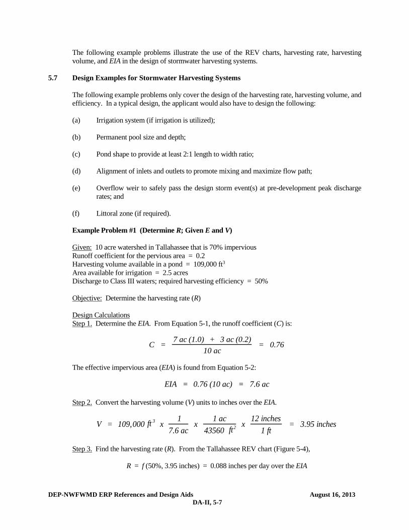
DEP-NWFWMD ERP References and Design Aids August 16, 2013 DA-II, 5-7
The following example problems illustrate the use of the REV charts, harvesting rate, harvesting volume, and EIA in the design of stormwater harvesting systems.
5.7 Design Examples for Stormwater Harvesting Systems
The following example problems only cover the design of the harvesting rate, harvesting volume, and efficiency. In a typical design, the applicant would also have to design the following: (a) Irrigation system (if irrigation is utilized); (b) Permanent pool size and depth; (c) Pond shape to provide at least 2:1 length to width ratio; (d) Alignment of inlets and outlets to promote mixing and maximize flow path; (e) Overflow weir to safely pass the design storm event(s) at pre-development peak discharge
rates; and (f) Littoral zone (if required).
Example Problem #1 (Determine R; Given E and V) Given: 10 acre watershed in Tallahassee that is 70% impervious Runoff coefficient for the pervious area = 0.2 Harvesting volume available in a pond = 109,000 ft3 Area available for irrigation = 2.5 acres Discharge to Class III waters; required harvesting efficiency = 50% Objective: Determine the harvesting rate (R) Design Calculations Step 1. Determine the EIA. From Equation 5-1, the runoff coefficient (C) is:
C = 7 ac (1.0) + 3 ac (0.2)
10 ac = 0.76
The effective impervious area (EIA) is found from Equation 5-2:
EIA = 0.76 (10 ac) = 7.6 ac
Step 2. Convert the harvesting volume (V) units to inches over the EIA.
V = 109,000 3ft x 1
7.6 ac x
1 ac43560 2ft
x 12 inches
1 ft = 3.95 inches
Step 3. Find the harvesting rate (R). From the Tallahassee REV chart (Figure 5-4),
R = f (50%, 3.95 inches) = 0.088 inches per day over the EIA

DEP-NWFWMD ERP References and Design Aids August 16, 2013 DA-II, 5-8
Step 4. Convert the harvesting rate units to inches per week over the irrigated area.
dayft =
inches 12ft 1 x
ac 1ft 43560 x ac 7.6 x
dayinch 80.0 = R
32
428,28
week
inches 1. = ft 1
inches 12 x ft 43560
ac 1 x ac 2.5
1 x week1days 7 x
dayft = R 2
3
87428,2
Therefore, irrigation of 1.87 inches per week over the 2.5 acre irrigation area will achieve 50% efficiency with the given harvesting volume.
Example Problem #2 (Determine V; given E and R)
Given: 20 acre watershed in Apalachicola that is 50% impervious Pervious C = 0.3 9 acres are available for irrigation at a rate of 2 inches per week Discharge to OFW; required efficiency is 90% Objective: Determine the harvesting volume (V) Design Calculations Step 1. Determine the EIA. From Equation 15-1, the runoff coefficient (C) is:
C = 10 ac (1.0) + 10 ac (0.3)
20 ac = 0.65
The equivalent impervious area (EIA) is found from Equation 15-2:
EIA = 0.65 (20 ac) = 13 ac
Step 2. Convert the harvesting rate units to inches per day over the EIA.
EIA the on day
inches 0.1 = days 7
week1 x ac 13
1 x week1inches 2 x ac = R 99
Step 3. Find the harvesting volume (V). From the Apalachicola REV chart (Figure 5-1),
V = f (90%; 0.19 inches/day over the EIA) = 6.5 inches over the EIA
Step 4. Convert the harvesting volume (V) units to ft3
ft 735306 = ac 1
ft 43560 x inches 12
ft 1 ac 13 x inches 6.5 = V 32
,
Therefore, 306,735 ft3 of harvesting volume is needed in the pond.

DEP-NWFWMD ERP References and Design Aids August 16, 2013 DA-II, 5-9
Example Problem #3 (Determine E; Given R and V)
Given: 3.5 acre watershed in Tallahassee that is 100% impervious Harvesting volume (V) = 0.875 ac-ft 2.87 acres are available for irrigation at a rate of 1.75 inches per week Objective: Determine the harvesting efficiency (E)
Design Calculations Step 1. Determine the EIA. Since the site is 100% impervious, the EIA = 3.5 acres Step 2. Convert the harvesting volume (V) units to inches over the EIA.
V = 0.875 ac - ft x 1
3.5 ac x
12 inches1 ft
= 3 inches on the EIA
Step 3. Convert the harvesting rate units to inches per day over the EIA.
R = 2.87 ac x 1.75 inches
1 week x
13.5 ac
x 1 week7 days
= 0.205 inches
day on the EIA
Step 4. Determine the efficiency from the Tallahassee REV chart (Figure 5-4).
E = f (0.205 inches/day; 3.0 inches) = 81%

DEP-NWFWMD ERP References and Design Aids August 16, 2013 DA-II, 6-1
6.0 Methodology and Design Example for Vegetated Natural Buffer Systems
The required width of a vegetated natural buffer (VNB) can be determined by overland sheet flow of runoff through the buffer (see Figure 11-1 in the NWFWMD Volume II for a schematic of a typical VNB). A minimum 25 foot buffer width must be specified.
6.1 Design Methodology for Calculating Buffer Width Based on Overland Flow
For systems which discharge to Class III receiving water bodies, the VNB must be designed to provide at least 200 seconds of travel time by overland flow through the buffer for the 2-year, 24-hour storm. Systems with direct discharges to OFWs, must be designed to provide at least 300 seconds of travel time by overland flow through the buffer for the 2-year, 24-hour storm. For overland sheet flow of less than 300 feet, Manning's kinematic solution (SCS 1986) to compute travel time (Tt) through the buffer is given by:
tT = 0.007 (n W 0.8)
( 2P 0.5) 0.4S (6-1)
where: Tt = Travel time (hr) n = Manning's roughness coefficient W = Buffer width (ft) P2 = 2-year, 24-hour rainfall depth (in) S = Slope of the hydraulic grade line (land slope) (ft/ft) This simplified form of the Manning's kinematic solution is based on the following (SCS 1986): (a) Shallow steady uniform flow (b) Constant intensity of rainfall excess (that part of a rain available for runoff) (c) Rainfall duration of 24 hours (d) Minor effect of infiltration on travel time Values for the 2-year, 24-hour storm can be obtained from Figure 2.7-1 in the NWFWMD Volume II. Values of Manning's roughness coefficient (n) for sheet flow can be obtained from Table 6-1, below.
Equation 16-1 can be rearranged to solve for the buffer width (W):
W = ( tT 1.25) ( 2P 0.625) 0.5S
0.002 n (6-2)
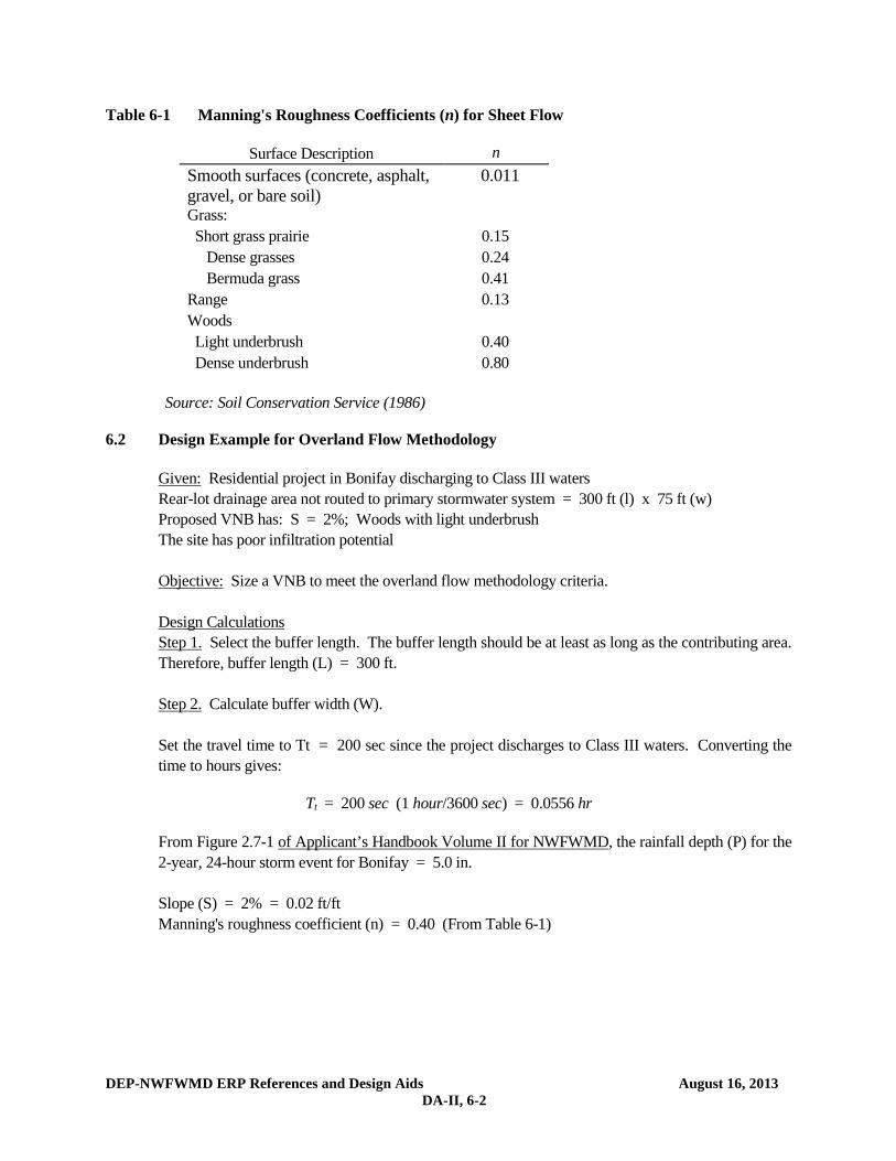
DEP-NWFWMD ERP References and Design Aids August 16, 2013 DA-II, 6-2
Table 6-1 Manning's Roughness Coefficients (n) for Sheet Flow
Surface Description n Smooth surfaces (concrete, asphalt, gravel, or bare soil)
0.011
Grass: Short grass prairie 0.15 Dense grasses 0.24 Bermuda grass 0.41 Range 0.13 Woods Light underbrush 0.40 Dense underbrush 0.80
Source: Soil Conservation Service (1986) 6.2 Design Example for Overland Flow Methodology
Given: Residential project in Bonifay discharging to Class III waters Rear-lot drainage area not routed to primary stormwater system = 300 ft (l) x 75 ft (w) Proposed VNB has: S = 2%; Woods with light underbrush The site has poor infiltration potential Objective: Size a VNB to meet the overland flow methodology criteria. Design Calculations Step 1. Select the buffer length. The buffer length should be at least as long as the contributing area. Therefore, buffer length (L) = 300 ft. Step 2. Calculate buffer width (W). Set the travel time to Tt = 200 sec since the project discharges to Class III waters. Converting the time to hours gives:
Tt = 200 sec (1 hour/3600 sec) = 0.0556 hr
From Figure 2.7-1 of Applicant’s Handbook Volume II for NWFWMD, the rainfall depth (P) for the 2-year, 24-hour storm event for Bonifay = 5.0 in. Slope (S) = 2% = 0.02 ft/ft Manning's roughness coefficient (n) = 0.40 (From Table 6-1)

DEP-NWFWMD ERP References and Design Aids August 16, 2013 DA-II, 6-3
The buffer width (W) can be determined from equation 6-2:
W = (0.0556 1.25) (5.0 0.625) (0.02 0.5)
0.002 (0.40)
W = 13.0 ft
Since the required minimum buffer width of 25 ft is greater that the width calculated above, set the buffer width (W) = 25 ft

DEP-NWFWMD ERP References and Design Aids August 16, 2013 DA-II, 8-1
7.0 Guidance for Stormwater Management System Retrofit Activities A typical retrofit project provides water quality treatment and/or flood storage/attenuation for a drainage area where no, minimal, or otherwise substandard control of stormwater management currently exists. By doing so, a properly designed retrofit project will reduce the pollutant loads discharged to a receiving waterbody, reduce flooding, or both. Therefore, retrofit projects have the potential to achieve substantial benefits to the water resources. Typically the area available for construction of the retrofit system is very limited and it is not possible to provide a treatment system that can meet the presumptive design and performance standards of a new development project. Retrofit projects are not intended to serve new development, redevelopment, or new sources of pollutant load discharges. Therefore the engineering design standard for a stormwater quality retrofit project is a demonstration that the project will result in a net reduction of pollutant loading to the receiving waterbody. The engineering design standard for a stormwater quantity (flood control) retrofit project is a demonstration that the project will reduce flooding without causing a net reduction in water quality treatment provided by the existing stormwater management system and without increasing discharges of untreated stormwater entering adjacent or receiving waters. The local, regional, or state agency proposing a retrofit project is encouraged to coordinate with the permitting FDEP or WMD agency early in the design process of the proposed retrofit project, pre-application meetings and field visits are encouraged. Recognizing the benefits that retrofit projects can provide to the water resources, the permitting agency will expedite, to the maximum extent practicable, the processing and technical review of an application for a retrofit project. More detail on stormwater retrofit projects is contained in section 2.8 of Volume II.

DEP-NWFWMD ERP References and Design Aids August 16, 2013 DA-II, 8-1
8.0 Flexibility for State Transportation Projects and Facilities State linear transportation projects and facilities (collectively referred to as “projects” in this section) often have unique design limitations. In recognition of this, subsection 373.413(6), F.S. (2012), requires the Agency to consider and balance the expenditure of public funds for stormwater treatment with the benefits to the public in providing the most cost-efficient and effective method of achieving the treatment objectives of stormwater management systems when reviewing such projects. To accomplish this, alternatives to on-site treatment for water quality will be considered including regional stormwater treatment systems, off-site compensating treatment, and incorporation of off-site runoff into the treatment system for the project. The incorporation or comingling of off-site runoff into the treatment system for the project is often a more cost effective design when compared to routing off-site runoff around the system. In most cases the comingling of off-site stormwater runoff into the system will also provide for increased pollutant removal when compared to the design option of routing it around the system even if the system is designed to only meet the design and performance standards of Volume II for the runoff from just the on-site project area. However, under some comingling conditions, the design capacity of the on-site system may need to be enlarged in order to provide at least the same level of water quality treatment as if the stormwater runoff was segregated and only runoff from the on-site project area was treated. Although this potential should always be evaluated to some degree in the design, it is an especially important design consideration when the off-site contributing area is much larger than the on-site project area and the expected concentrations of pollutants from the off-site areas are significantly less that those expected by the on-site project area, or when retention-type BMPs are selected.