residential land recapitalization
TRANSCRIPT

1
REAL 899: Seevak Research Competition Professor Gyourko
Residential Land Recapitalization “Equity Returns for Debt Risk”
Larry Burnett, Caroline Jones, Adam Krug
2
1. Introduction The housing sector stands at the end of a significant boom after its cyclical bottom in the
mid-1990s. Housing is driven by multiple factors – inflation, income growth,
construction costs, demographics and interest rates – each of which play greater or lesser
roles at different times. A recent study by PPR shows that the boom over the past 10
years divides broadly into two phases nationwide: an uneven boom in the late 1990s that
drove prices up in regions with superior economic performance such as the San Francisco
Bay Area and the Northeastern United States. This was followed by an interest-rate
driven boom that drove asset prices more broadly from 2001 to 2006. While economic
growth continues, higher short-term interest rates have weakened housing demand and
brought an end to the recent housing boom. There is concern that an upward spike in
interest rates or a faltering economy could send housing prices plummeting.
Much has been made of the recent bursting of the US housing bubble, specifically in the
coastal markets that have seen the highest appreciation. The evidence of the burst lies in
significant homebuilder write-offs, flat or declining median home prices, longer average
time on the market, and increases in months supply of new home inventory. After
dramatic price increases and unit supply surges in single family and multi family
residential dwelling units over the last 5 years, the broader market contraction in unit
home sales and specific submarket contraction in home values has led to popular
consensus questioning the potential and security of residential investment. Yet a closer
investigation of the drivers of residential asset values, as well as a careful evaluation of
today’s environment in historical context, reveals residential investment opportunities.

3
The broader housing market correction has led to inefficient asset capitalization:
Homebuilders are holding too much land at inflated prices and as they write those assets
down and walk away from land options, their debt ratios and coverage ratios are higher
than they would like at a time when earnings are falling. Small, medium and large banks
with significant corporate lending exposure to homebuilders, sub-prime mortgages and
the housing sector in general, are re-evaluating their underwriting of housing related debt
and in some cases are looking for partial or full repayments from the borrowers.
Homebuilders are now seeking to strengthen their balance sheets through the sale of
assets and reduction in corporate debt. However, they still need access to capital for
ongoing development of projects. As a result they are looking to restructure certain assets
and liabilities to be “off balance sheet,” thus achieving both goals.
Our investment premise is to solve the liquidity problem for both lenders and borrowers,
by stepping in to offer non-recourse debt to the homebuilder, with land as the collateral.
This allows the homebuilder to refinance existing debt and eliminate parent company
recourse, it allows the lending bank to reduce its sector and homebuilder specific
exposure, and it allows us to earn outsized returns relative to the risk taken.
Our investment strategy relies on the careful selection of land because in the event of a
default we must be comfortable holding the land as collateral. Much of this paper builds
the case around specific target submarkets. We believe that we can earn excellent returns
because we are willing to take a contrarian position and hold land at a time when most
participants in the industry want to reduce their land exposure. We are prepared to hold

4
the land 3-5 years, during which time we are confident the markets we select will
rebound.
Within this context, where in the country would an investor have the greatest comfort
holding residential land? Given that the national interest rate environment affects all
local markets, non-interest rate related drivers of housing value are critical factors to
consider. These include population, income and job growth (factors that drive demand) as
well as geographic limitations and regulatory barriers (factors that constrain supply). Our
investment strategy is focused on California, a state that excels in these drivers of long-
term real estate value. We also chose Dallas as a contrasting market to analyze because of
its nature as a relatively unconstrained supply market in a non-coastal region.
Methodology
In this report we first explain our proposed transaction in detail covering both a base case
and downside scenario and sensitivity analysis around our assumptions. We then build
the case that there is demand among homebuilders and lenders for the financing that we
propose. Finally we explore three markets: Greater Los Angeles, CA, the San Francisco
Bay Area, CA, and Dallas-Fort Worth, TX. We are looking for the most attractive
markets based on quantifiable, tangible evidence that makes us comfortable holding land
if our borrower defaults on the loan. Specifically, we are looking for (1) Entitled land in
submarkets where the permitting process is laborious and where supply of new homes is
constrained; (2) Submarkets with decent long-term demand drivers such as above average

5
population and income growth; and (3) Submarkets where prices have already started to
correct.

6
2. Transaction Details
Our target transaction involves recapitalizing an existing project that has gone though the
entitlement machinery and has an approved specific plan and tentative tract map. We
conservatively underwrite the value of land and lend money against such collateral. The
homebuilder retains equity in the project and, ideally, there is new joint venture equity
invested in the project at the time of our recapitalization, although we have not assumed
this is the case.
We—for clarity we will call ourselves New Lender, Inc—address the desire of existing
lenders to reduce their exposure by purchasing their project-specific debt at or below face
value. New Lender, Inc. allows the existing lender to remain invested at a more
comfortable basis by borrowing back 50% of their prior loan amount, but with only our
first mortgage as their collateral rather than an upstream guaranty from New Lender, Inc
or a corporate guaranty from the homebuilder. New Lender, Inc then negotiates with the
homebuilder to increase the interest rate of the note in exchange for making it
collateralized on an asset specific basis and not subject to a corporate balance sheet
guaranty. This allows the homebuilder to remove the debt from its balance sheet and in
return they are willing to pay a higher interest rate. We source deals through lenders and
builders in select markets and will target situations where new joint venture equity is
being invested. See Exhibit 1 for the flow diagram.

7
Exhibit 1: Transaction flow diagram
Homebuilder We restructure the
loan with Borrower to LIBOR +450 and non-
recourse. Borrower gets debt off balance
sheet.
Original LenderBank lends $50mm to us (LIBOR +250) thus
maintaining some exposure to transaction.
New Lender We purchase $100mm
loan (LIBOR +250) from Original Lender (backed by Borrower
parent company guarantee).
$100mm
$100mm
$50mm
$50mm Equity
$50mm
We invest $50 mm of our own and borrow $50mm from the bank.
Bank reduces net exposure by $50mm.
Why it works: The borrower wants non-recourse debt, the bank wants to decrease
exposure to sector/builder, and we are comfortable holding the land as collateral.
Transaction structure
• We appraise the project value to reflect the current environment. In this case we
have assumed that the total project capitalization has fallen 5% from $150mm to
$142.5mm, of which $42.5mm is homebuilder equity and $100mm is the loan
amount.
• We purchase the existing $100mm loan from the lending bank at or below par; we
pay par value only in the lowest (<50%) Loan to Value situations.

8
• We invest $50mm of our own money and borrow the other $50mm from the
lending bank (so that they are now lending to us instead of to the homebuilder and
they are only lending $50mm instead of $100mm, thus reducing their exposure).
• We leverage our returns by borrowing that $50mm at LIBOR +250bp and lending
it to the homebuilder at LIBOR +450bp, thus earning a spread of 200bp on the
$50mm “borrowed back” amount.
• The bank is willing to lend to us at LIBOR +250bp because they have reduced
their exposure by 50% and effectively have another significant equity investor
behind them in the capital structure.
• We revise terms with homebuilder to remove parent company recourse and
increase the interest rate by 200bp to LIBOR +450bp. The homebuilder is willing
to accept a higher interest rate to get the debt off the balance sheet. We think this
interest rate spread is a reasonable estimate because:
o The top 10 homebuilders current loan spreads range from senior debt of
100+ bps to subordinated debt spreads of 400+ bps over LIBOR.
o We have assumed a midpoint base rate of LIBOR + 250
o Both large and small builders are willing to pay for off balance sheet
financing, a true sub debt spread is appropriate.
• The loan collateral is the entitled land and improvements value, underwritten to
conservative loan to value ratios (<70%). In other words, our investment is now
backed by specific project assets instead of by total company assets.

9
Exhibit 2: Transaction Assumptions and Structure Original Project- Pre Recapitalization ($ in 000s)Homebuilder Invested Equity: Existing Land and Improvements Loan: Total Project Capitalization:$50,000 $100,000 @ LIBOR + 250 (currently 7.8%) $150,000
Fully recourse to Homebuilder
Valuation at Closing of Recapitalization ($ in 000s)Homebuilder Equity Value: New Land and Improvements Loan: Total Project Capitalization:$42,500 $100,000 @ LIBOR + 450 (currently 9.8%) $142,500assumes 15% equity writedown (based on appraisal) assuming purchase at par (worst case)assumes no new equity (worst case) collateralized only by projectassumes 70% LTV (worst case)
Borrow Back from Original Lender ($ in 000s)New Lender's Invested Equity: Original Lender's loan to New Lender: Total New Lender Capitalization:$50,000 $50,000 @ LIBOR + 250 $100,000
New Implied LTVs 50% on Loan Sale and 35% on ultimate collateral
Base case scenario:
• We anticipate repayment of debt by borrower over a 3-5 year investment horizon.
• In this example we assume New Lender, Inc. receives interest for 3 years, with
repayment of the principal amount at the end of Year 3.
• New Lender, Inc. generates an interest rate spread of 200bps between the original
lending bank and the new loan to the homebuilder.
• This generates an IRR of 11.18% over the three year period.
• This yields a positive $4.38mm NPV at our estimated WACC of 7.8% (our
assumed borrowing rate), including underwriting and closing costs of $750,000
for our business.

10
Exhibit 3: Base Case Cash Flow and Return Assumptions BASE CASE SCENARIO ($ in 000s)New Investment Cash Flow: Closing Year 1 Year 2 Year 3 Year 4 Year 5 TotalPayoff Original Lender at par- 70% LTV ($100,000) ($100,000)Underwriting, Closing Costs ($750)Change Interest rate to LIBOR + 450 $9,800 $9,800 $9,800 $0 $0 $29,400Principal repayment by Borrower $0 $0 $100,000 $0 $0 $100,000Borrow 50% from Original Lender $50,000 $50,000Interest to Original Lender @ LIBOR + 250 ($3,900) ($3,900) ($3,900) $0 $0 ($11,700)Principal repayment to Original Lender $0 $0 ($50,000) $0 $0 ($50,000) Cash Flow to New Lender ($50,750) $5,900 $5,900 $55,900 $0 $0 $16,950 IRR 11.18% NPV using 7.8% discount rate $4,376
Downside case scenario:
• The borrower defaults after Year 1 and New Lender, Inc. forecloses in Year 2.
• The carry costs are 2% of original value, annually (property taxes, legal,
maintenance).
• New Lender, Inc. sells the assets in Year 5.
• We assume that the assets are sold at the originally underwritten value
($142.5mm), which was already written down 5% in the original appraisal. In
other words, we assume no nominal appreciation in land value over a five year
time period. We consider this a conservative assumption.
• Our downside assumptions yield an IRR of 6.74% which is slightly below our
cost of capital, and therefore negative NPV.
• Because we only lend up to 70% of the value ($100mm/142.5mm), the assets
could depreciate another 15% at time of sale before our project is cash flow
negative.
• We consider this an acceptable downside scenario with conservative assumptions.

11
Exhibit 4: Downside Case Cash Flow and Return Assumptions Default Event Q1 Land Sale
DOWNSIDE CASE SCENARIO ($ in 000s) Foreclose Q4 EventNew Investment Cash Flow: Closing Year 1 Year 2 Year 3 Year 4 Year 5 TotalPayoff Original Lender at par- 70% LTV ($100,000) ($100,000)Underwriting, Closing Costs ($750)Change Interest rate to LIBOR + 450 $9,800 $0 $0 $0 $0 $9,800Principal repayment by Borrower $0Taxes, Legal and Carry Costs @ 2% of original underwritten value ($2,850) ($2,850) ($2,850) ($2,850) ($11,400)Land and Improvements Sale @ 100% of original underwritten value $0 $0 $0 $142,500 $142,500Borrow 50% from Original Lender $50,000 $50,000Interest to Original Lender @ LIBOR + 250 ($3,900) ($3,900) ($3,900) ($3,900) ($3,900) ($19,500)Principal repayment to Original Lender $0 $0 $0 $0 ($50,000) ($50,000) Cash Flow to New Lender ($50,750) $5,900 ($6,750) ($6,750) ($6,750) $85,750 $20,650 IRR 6.74% NPV using 7.8% discount rate ($2,648)
Sensitivity Analysis
Base case: We test our assumptions by conducting sensitivity analysis on our key
assumptions. As you can see in Exhibits 5 and 6, in our base case scenario, if we are
unable to generate a 200bp spread on the “borrowed back” amount, we still anticipate
generating positive NPV at as low as a 50bp spread, at our 7.8% discount rate. If we can
purchase the original loan at a value below par then our returns should be higher than our
base case assumptions.
Exhibit 5: IRR Sensitivity assuming 3 year payback Exhibit 6: NPV Sensitivity 3 year payback, purchase at Par
Interest Spread in Basis Points (Rate Charged to Borrower vs paid to Lender)
11.18% 50 100 150 200 250$80,000 21.4% 22.3% 23.2% 24.1% 25.0%
Loan $85,000 17.9% 18.8% 19.7% 20.6% 21.5%Purchase $90,000 14.5% 15.4% 16.4% 17.3% 18.2%
Price $95,000 11.3% 12.3% 13.2% 14.2% 15.1%$100,000 8.2% 9.2% 10.2% 11.2% 12.2%
(Rate Charged to Borrower vs paid to Lender)$4,376 50 100 150 200 250
6.0% $2,992 $4,329 $5,665 $7,002 $8,338Discount 7.0% $1,612 $2,924 $4,236 $5,548 $6,861
Rate 8.0% $281 $1,569 $2,858 $4,146 $5,4359.0% ($1,003) $263 $1,528 $2,794 $4,059
10.0% ($2,242) ($999) $245 $1,488 $2,732
Downside Case sensitivity: As we show in Exhibits 7 and 8, if we can sell the land after
five years at above the original value, then our returns will be higher and conversely if
the sale price is lower, then the IRR and NPV will be lower. Later in this report we

12
discuss land as an investment class and how we plan to mitigate our risk by careful
selection of each submarket. Because of these factors we view it as very unlikely that we
would be forced to sell at below original value in five years.
Exhibit 7: IRR Sensitivity assuming Default and Foreclosure in Year 2, Land Sale in Year 5
Exhibit 8: NPV Sensitivity assuming 2% carry Costs, sale in Year 5
Carry Costs as % of Original Underwritten Value6.74% 1.0% 1.5% 2.0% 2.5% 3.0%
Land 90.0% 4.3% 3.3% 2.3% 1.3% 0.2%Sale % of 95.0% 6.5% 5.5% 4.6% 3.6% 2.7%Original 100.0% 8.6% 7.6% 6.7% 5.8% 4.9%
Value 105.0% 10.5% 9.6% 8.7% 7.9% 7.0%110.0% 12.3% 11.4% 10.6% 9.7% 8.9%
Discount Rate($2,648) 6.0% 7.0% 8.0% 9.0% 10.0%
Land 90.0% ($8,777) ($10,813) ($12,732) ($14,543) ($16,251)Sale % of 95.0% ($3,452) ($5,733) ($7,883) ($9,912) ($11,827)Original 100.0% $1,872 ($653) ($3,034) ($5,281) ($7,403)
Value 105.0% $7,196 $4,427 $1,815 ($650) ($2,979)110.0% $12,520 $9,507 $6,664 $3,981 $1,446
Risk mitigation: Careful underwriting of the collateral value is critical to mitigate the
risk of our investment. We carefully select submarkets by understanding the key supply
and demand drivers of land, and ultimately home values in those markets. We note that
land is a more volatile asset class than housing (see Exhibit 9). We plan to take advantage
of this price volatility by focusing on regions where prices have already started to correct.
In addition, we cap our loan value at 70% of asset price. We choose entitled land in areas
where the regulatory process is long because we think entitled land prices will bounce
back the quickest when the market improves. Finally, we have the ability and willingness
to hold the land for 3-5 years to see the market through the down cycle.
We note that in the PWC/ULI “Emerging Trends in Real Estate” survey for 2006
(conducted in late 2005), land registered the highest expected return of all real estate
asset classes at 10.9% (Appendix: Exhibit 1), on the back of the long housing boom.

13
Exhibit 9: Volatility of Land, Home and Structure Prices, 1977-2005 (year/year changes in real values): Land is a more volatile asset class.
Drawn from: PPR, “Land as an Investment Class,” Oct. 2006, p. 5.
14
3. The Disconnect Between Homebuilders and Lenders
We believe there is a market for the transaction just described because there is a
fundamental disconnect between homebuilders and lenders at the current time.
Homebuilders’ balance sheets have weakened so they are looking to refinance projects to
move them off balance sheet. Lenders are finding themselves overexposed to the housing
sector in general and want to reduce their exposure to this sector. This provides a
financing need in the market, which we fill.
Homebuilder balance sheets have weakened. For the last several years homebuilders have
been dramatically increasing their investments in land assets (see Exhibits 10 and 11).
Now, with a downturn in the housing market, homebuilders are finding themselves with
more land than they want. As a result, they are walking away from options and writing
down the value of land on their balance sheets. With a reduction in assets and equity, net
debt positions have worsened at a time when sales are slowing and profits are declining.
A recent KB Homes’ press release is typical of the industry: "Net income and earnings
per share dropped sharply in the face of increasingly difficult market conditions….an
oversupply of unsold new and resale homes, reduced affordability, and greater caution
among potential homebuyers heightened competition among homebuilders and sellers of
existing homes, prompting the aggressive use of price concessions and sales incentives.
All these factors pressured our operating margins. Our results were further affected by
declining land values and the resulting charges we recorded.”

15
Exhibit 10. Homebuilders’ supply of land with no future growth
Exhibit 11: Homebuilders land investments have dramatically increased
The top 10 homebuilders have seen their trailing twelve month EBITDA decline by an
average of 48% year over year, or 44% excluding land and option writedowns. Because
of declining EBITDA, coverage ratios such as net debt/EBITDA ratios have worsened
significantly (see Exhibit 12). On average, the top 10 homebuilders net debt to trailing
twelve month EBITDA has increased from 1.6x to 4.1x, or 2.4x excluding the
writedowns. This drop in coverage ratios threatens debt covenants and makes raising
capital more difficult.
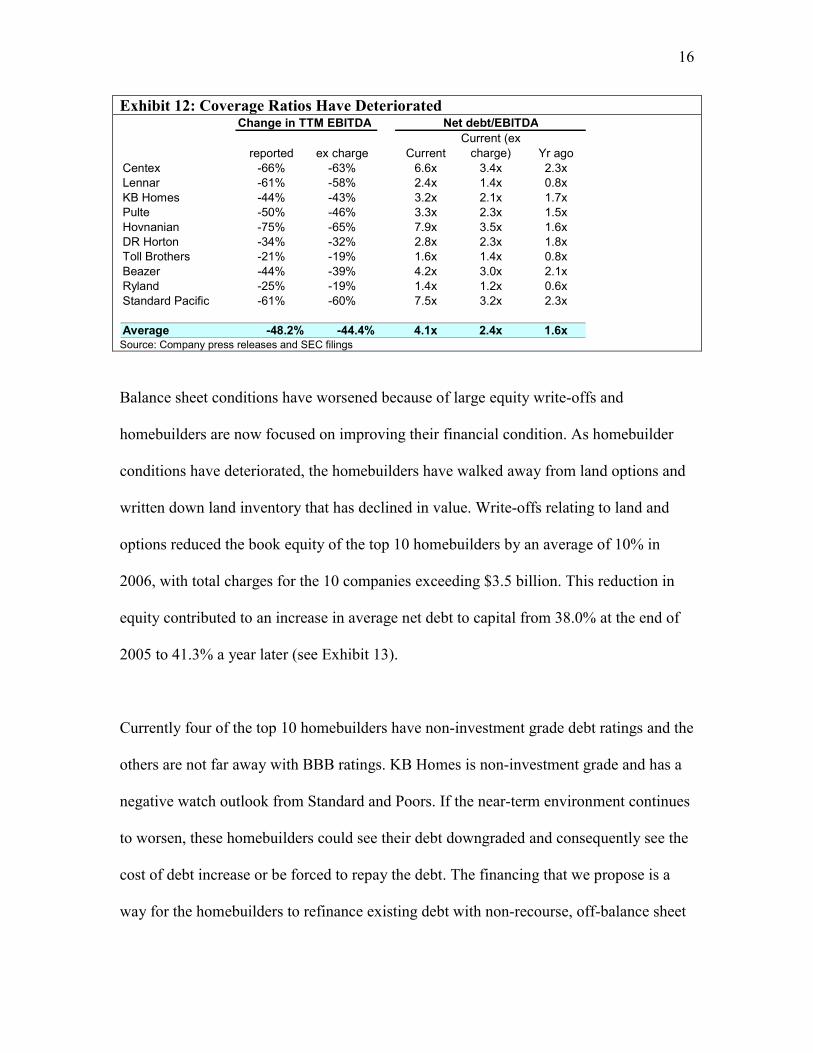
16
Exhibit 12: Coverage Ratios Have Deteriorated Change in TTM EBITDA Net debt/EBITDA
reported ex charge CurrentCurrent (ex
charge) Yr agoCentex -66% -63% 6.6x 3.4x 2.3xLennar -61% -58% 2.4x 1.4x 0.8xKB Homes -44% -43% 3.2x 2.1x 1.7xPulte -50% -46% 3.3x 2.3x 1.5xHovnanian -75% -65% 7.9x 3.5x 1.6xDR Horton -34% -32% 2.8x 2.3x 1.8xToll Brothers -21% -19% 1.6x 1.4x 0.8xBeazer -44% -39% 4.2x 3.0x 2.1xRyland -25% -19% 1.4x 1.2x 0.6xStandard Pacific -61% -60% 7.5x 3.2x 2.3x
Average -48.2% -44.4% 4.1x 2.4x 1.6x Source: Company press releases and SEC filings
Balance sheet conditions have worsened because of large equity write-offs and
homebuilders are now focused on improving their financial condition. As homebuilder
conditions have deteriorated, the homebuilders have walked away from land options and
written down land inventory that has declined in value. Write-offs relating to land and
options reduced the book equity of the top 10 homebuilders by an average of 10% in
2006, with total charges for the 10 companies exceeding $3.5 billion. This reduction in
equity contributed to an increase in average net debt to capital from 38.0% at the end of
2005 to 41.3% a year later (see Exhibit 13).
Currently four of the top 10 homebuilders have non-investment grade debt ratings and the
others are not far away with BBB ratings. KB Homes is non-investment grade and has a
negative watch outlook from Standard and Poors. If the near-term environment continues
to worsen, these homebuilders could see their debt downgraded and consequently see the
cost of debt increase or be forced to repay the debt. The financing that we propose is a
way for the homebuilders to refinance existing debt with non-recourse, off-balance sheet

17
financing, allowing them to maintain their debt ratings and improve the look of their
corporate balance sheets.
Exhibit 13: Net Debt / Capital Ratios have Increased Net debt/capital Debt ratings Writedown % of equity
Current Yr agoCentex 46.4% 45.9% BBB/Stable/A-2 11%Lennar 25.5% 24.3% BBB/Stable/-- 10%KB Homes 46.0% 45.5% BB+/Watch Neg/ 13%Pulte 36.6% 35.5% BBB/Stable/-- 7%Hovnanian 51.4% 42.4% BB/Stable/-- 15%DR Horton 41.2% 40.7% BBB-/Stable/-- 5%Toll Brothers 31.8% 27.6% BBB-/Stable/-- 4%Beazer 49.5% 47.1% BB/Stable 9%Ryland 32.7% 25.1% BBB-/Stable/-- 5%Standard Pacific 52.2% 46.5% BB/Stable/-- 17%
Average 41.3% 38.0% 4 less than BBB rated 10%Source: Press releases and SEC filings
One of the main priorities now for homebuilders is improving the strength of their
balance sheets. Centex’s fourth quarter 2006 earnings call is a typical example:
Management said “We're taking the necessary steps to get our balance sheet and our
organization to their fighting weight” and “We'll look seriously at debt repurchase as
necessary, again, given the realities of where earnings will go and to help strengthen our
balance sheet positioning for the future…..I'll emphasize that we're taking aggressive
steps to right size operations, reduce our costs, and strengthen our balance sheet.”
Other homebuilders have made similar comments in their earnings calls, press releases
and SEC filings. Balance sheet strength is a serious priority for the home builders.
However, they still need capital to continue developing the land they own in order to
generate sales and profits. This is why off-balance sheet financing is an attractive option
for them to recapitalize existing projects or raise capital to develop new projects.

18
There is also a market for our proposed homebuilding financing amongst lenders who
want to reduce their exposure to the housing sector. Declining home and land prices and
homebuilder equity write-downs means lenders are now protected by less collateral. And
as we have shown, homebuilders already have risky debt. As coverage ratios worsen
there may be covenant violations and ratings downgrades which could trigger forced debt
repayment. In addition, many lending banks are finding themselves over-exposed to sub-
prime mortgages and are looking to reduce their exposure to housing related debts as the
sub-prime market unravels. For example, HSBC has set aside more than $10.5 billion to
cover losses on its US sub-prime business. New Century Financial filed for bankruptcy
protection. Accredited Home Lenders Holding Co and General Motors Acceptance
Corp’s residential unit are both facing financial problems related to the sub-prime market
and their lenders – banks such as Bank of America and Citigroup – may want to decrease
their exposure to risky debt and pull back their exposure to the housing sector in general.
Our recapitalization transaction is a way for them to reduce this exposure.
The subprime fallout should actually be a net positive for us, however, because it has
forced credit spreads to widen on homebuilder debt because the risk associated with
homebuilders has risen. The subprime fallout reduces the potential pool of new home
buyers as risky mortgage applications are now turned down. It probably also makes
borrowing slightly tougher for prime mortgages as well. This dampens demand and
reduces the likelihood of a quick snap-back in the homebuilding market. The
homebuilders also have varying exposure to the mortgage market directly (including
subprime) and the higher debt yields reflect that. At the same time, the subprime fallout

19
increases the chance that the Federal Reserve eases rates, thus leading to a potential
widening of spreads on the kind of debt we are offering.
Obviously, a slower snap-back in the homebuilding market has risks for our strategy.
However, as we have outlined, we are prepared to hold the land for 3-5 years, and are not
counting on a quick snap-back. As long as the long-term supply and demand drivers are
in place, our strategy should work and now we can earn higher spreads on our risk. It also
means lenders are likely to be more interested in our proposed deal as well as they try to
reduce exposure to housing related debt. Net-net, the subprime fallout is probably good
for us.
Subprime degradation is likely to dampen demand for housing, not sink the market. This
is because subprime represents less than 10% of mortgages and there are no indications
of major problems in prime mortgages. At the end of 2006, only 1.2% of mortgages were
in foreclosure and only 5.1% of homeowners had a subprime mortgage. The biggest risk
is if falling home prices lead to a recession. Higher unemployment and lower personal
income could hamper prime mortgage holders’ ability to make mortgage payments and
put pressure on the housing market. However, the good news is that the economy looks
healthy (albeit with slowing growth): consumer spending has been resilient,
unemployment remains low, durable goods and manufacturing orders are increasing, and
corporate balance sheets (including those of banks) are strong.

20
There is evidence that homebuilders are increasing the sort of off-balance sheet debt and
equity financing, consistent with what we are proposing. Eight of the top 10
homebuilders disclosed joint venture debt in their SEC filings. These eight saw their total
unconsolidated joint venture debt increase 22% year over year to nearly $14 billion. Joint
venture debt and equity allows homebuilders to raise capital that they need to keep
developing properties while keeping it off their balance sheets, so that their coverage and
profitability ratios improve, which is what shareholders and lenders want.
For example, Lennar wrote in its most recent 10-K that it was admitting a new strategic
partner into its LandSource joint venture that will “result in a cash distribution to us and
our current partner, LNR, of approximately $660 million each….The new partner will
contribute cash and property with a combined value of approximately $900
million….Following the contribution and refinancing, our and LNR's interest in
LandSource will be diluted to 19% each, and the new partner will be issued a 62%
interest in LandSource.” Similarly, Standard Pacific management announced on a recent
analyst call “We expect to continue using joint venture structures for land development
and homebuilding equity and debt funding needs.”
In many cases, the off-balance sheet financing is raised by the homebuilder’s joint
venture partner. For example, KB Homes says in the company’s most recent 10-K “We
may also acquire land with seller financing that is non-recourse to us, or by working in
conjunction with third-party land developers” and Hovnanian writes “Typically, our
21
unconsolidated joint ventures obtain separate project specific mortgage financing for each
venture.”
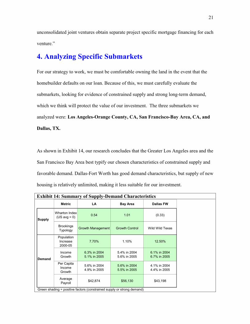
4. Analyzing Specific Submarkets
For our strategy to work, we must be comfortable owning the land in the event that the
homebuilder defaults on our loan. Because of this, we must carefully evaluate the
submarkets, looking for evidence of constrained supply and strong long-term demand,
which we think will protect the value of our investment. The three submarkets we
analyzed were: Los Angeles-Orange County, CA, San Francisco-Bay Area, CA, and
Dallas, TX.
As shown in Exhibit 14, our research concludes that the Greater Los Angeles area and the
San Francisco Bay Area best typify our chosen characteristics of constrained supply and
favorable demand. Dallas-Fort Worth has good demand characteristics, but supply of new
housing is relatively unlimited, making it less suitable for our investment.
Exhibit 14: Summary of Supply-Demand Characteristics Metric LA Bay Area Dallas FW
Supply
Wharton Index (US avg = 0) 0.54 1.01 (0.33)
Brookings Typology Growth Management Growth Control Wild Wild Texas
Population Increase 2000-05
7.70% 1.10% 12.50%
Demand
Income Growth
6.3% in 2004 5.1% in 2005
5.4% in 2004 5.6% in 2005
6.1% in 2004 6.7% in 2005
Per Capita Income Growth
5.6% in 2004 4.9% in 2005
5.6% in 2004 5.5% in 2005
4.1% in 2004 4.4% in 2005
Average Payroll $42,874 $56,130 $43,198
Green shading = positive factors (constrained supply or strong demand)

22
Supply factors
Coastal California is an attractive market from a supply perspective with land
geographically constrained and development burdened by a lengthy regulatory process.
Greater Los Angeles is an urban area geographically bounded on two sides by mountains
and on one side by the ocean. The remaining side merges into another strong performing
submarket, Orange County. San Francisco and San Jose are similarly constrained by
geography (ocean and bay), limited available land for development, and generally
restrictive permitting. For example, San Mateo County, located in between San
Francisco and San Jose, has 350,000 jobs, but between 1999 and 2005 built on average
1050 new housing units per year (Bay Area Council, “Bay Area Housing Profile 2006,” pp 37-
39). This limited supply in the West Bay drives development toward the East Bay, where
geographical and legal constraints are fewer. This is where most of the new housing
developments are occurring (and consequently where our investment idea is focused).
Despite an easier supply environment in the East Bay, the overall Bay Area taken as a
whole has limited supply that has failed to keep up with demand and we think this
dynamic will continue to support land prices in the area.
From a regulatory perspective, zoning, affordable housing requirements, permit caps,
containment boundaries, and other infrastructure management rules further restrict the
available developable land in California and make the permitting process long, expensive
and complex. There have been two recent studies which developed frameworks to assess
regulatory constraints on development throughout the country: both ranked Los Angeles-
Orange County and San Francisco Bay Area regions as highly regulated.

23
The Brookings Institute’s approach to regulatory land use typologies found that Southern
California used affordability requirements, containment policies and infrastructure
management as extensions of zoning. The Bay Area additionally used permit caps to
limit growth. The Wharton Residential Land Use Regulatory Index looks specifically at a
number of housing-related regulations: San Francisco Bay Area ranked extremely high at
1.01 and Los Angeles ranked high at 0.54 versus a national average of 0.00. In contrast,
Dallas ranked well below average at (0.33) indicating a much easier development
environment (See Exhibit 15). As one researcher noted, “California represents the most
extreme example of autarky in land-use regulations of any U.S. state. Cities are free to
set their rules independently, with little oversight.” (Quigly/Raphael, p 323).
Exhibit 15: Brookings Institute shows California as a Restrictive Market for Development in Contrast to Texas which is “Wild Wild West” Easy Development.
Source: Pendall, Rolf et. al., “From Traditional to Reformed: A Review of the Land Use Regulations in the Nation’s 50 largest Metropolitan Regions,” The Brookings Institution, Aug. 2006.

24
In Los Angeles-Orange County, the lengthy development approval processes and
prohibitive local statutes create a dangerous time spectrum of uncertainty for developers
and discourage new market entrants. As an example of local legal constraints, in 1998
Ventura County enacted the SOAR “Save Our Agricultural Resources” initiative, which
prohibited any owner of open space, rural or agriculturally zoned land to even apply for
re-zoning until 2017. Furthermore, restrictions on maximum allowable slope, in an area
with significant topographic challenges, serve to limit development potential even on
residentially zoned land.
Under-supply of new homes logically contributes to higher home prices in California. A
recent study data from the 1990s (Quigley/Raphael, 2005), showed a clear correlation
between restrictive zoning and higher housing prices in California. As a result of
restrictive regulations and geographic constraints, California housing production has
fallen short of demand for housing (Exhibits 16, 17, and 18). In Greater Los Angeles,
only one new unit is produced for every 4 new residents and housing permits have
significantly lagged job creation. In the San Francisco Bay Area, there is a 13% deficit in
new home production, (assuming one housing unit is produced for every 1.5 new jobs
created, which is the regional average).

25
Exhibit 16: Southern California Supply of New Housing has Lagged Population Growth
Exhibit 17: SF-Bay Area Housing versus Demand: Net Deficit of Housing Supply
18: Housing production has not kept pace with jobs
Source: SCAG, 2001
Source: Bay Area Council
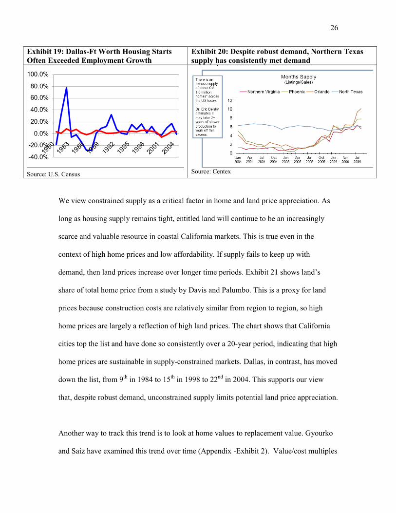
In contrast, Dallas has seen housing unit growth often exceed job growth (Exhibit 19).
Exhibit 20 shows how supply in North Texas (DFW) is very flexible, so that strong
demand is met by an immediate supply response and overall housing supply as measured
by inventory-to-sales, remains constant. The result is that housing is truly a consumer
good, matching income-driven demand over time. This implies little opportunity for land
appreciation over time. This is consistent with lots of available land and limited
restrictions on development.
26
Exhibit 19: Dallas-Ft Worth Housing Starts Often Exceeded Employment Growth
Exhibit 20: Despite robust demand, Northern Texas supply has consistently met demand
-40.0%
-20.0%
0.0%
20.0%
40.0%
60.0%
80.0%
100.0%
1980
1983
1986
1989
1992
1995
1998
2001
2004
Source: U.S. Census Source: Centex
We view constrained supply as a critical factor in home and land price appreciation. As
long as housing supply remains tight, entitled land will continue to be an increasingly
scarce and valuable resource in coastal California markets. This is true even in the
context of high home prices and low affordability. If supply fails to keep up with
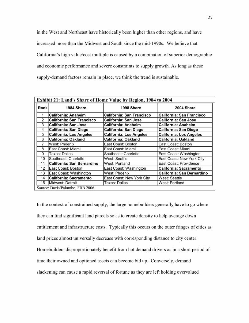
demand, then land prices increase over longer time periods. Exhibit 21 shows land’s
share of total home price from a study by Davis and Palumbo. This is a proxy for land
prices because construction costs are relatively similar from region to region, so high
home prices are largely a reflection of high land prices. The chart shows that California
cities top the list and have done so consistently over a 20-year period, indicating that high
home prices are sustainable in supply-constrained markets. Dallas, in contrast, has moved
down the list, from 9th in 1984 to 15th in 1998 to 22nd in 2004. This supports our view
that, despite robust demand, unconstrained supply limits potential land price appreciation.
Another way to track this trend is to look at home values to replacement value. Gyourko
and Saiz have examined this trend over time (Appendix -Exhibit 2). Value/cost multiples
27
in the West and Northeast have historically been higher than other regions, and have
increased more than the Midwest and South since the mid-1990s. We believe that
California’s high value/cost multiple is caused by a combination of superior demographic
and economic performance and severe constraints to supply growth. As long as these
supply-demand factors remain in place, we think the trend is sustainable.
Exhibit 21: Land's Share of Home Value by Region, 1984 to 2004
1 California: Anaheim California: San Francisco California: San Francisco2 California: San Francisco California: San Jose California: San Jose3 California: San Jose California: Anaheim California: Anaheim4 California: San Diego California: San Diego California: San Diego5 California: Los Angeles California: Los Angeles California: Los Angeles6 California: Oakland California: Oakland California: Oakland7 West: Phoenix East Coast: Boston East Coast: Boston8 East Coast: Miami East Coast: Miami East Coast: Miami9 Texas: Dallas Southeast: Charlotte East Coast: Washington10 Southeast: Charlotte West: Seattle East Coast: New York City11 California: San Bernardino West: Portland East Coast: Providence12 East Coast: Boston East Coast: Washington California: Sacramento13 East Coast: Washington West: Phoenix California: San Bernardino14 California: Sacramento East Coast: New York City West: Seattle15 Midwest: Detroit Texas: Dallas West: Portland
1984 ShareRank 1998 Share 2004 Share
Source: Davis/Palumbo, FRB 2006
In the context of constrained supply, the large homebuilders generally have to go where
they can find significant land parcels so as to create density to help average down
entitlement and infrastructure costs. Typically this occurs on the outer fringes of cities as
land prices almost universally decrease with corresponding distance to city center.
Homebuilders disproportionately benefit from hot demand drivers as in a short period of
time their owned and optioned assets can become bid up. Conversely, demand
slackening can cause a rapid reversal of fortune as they are left holding overvalued

28
inventory. The current homebuilding environment exemplifies demand slackening and
the spoken desire to reduce land holdings.
Yet, we believe that careful selection of submarkets can minimize the downward pricing
pressure during broader market corrections. Underwriting the value of land in certain
markets requires knowledge of the entitlement and development processes and in-place
approvals, historical perspective on pricing, competition, and the various economic
factors at play.
A closer look at where homebuilder pain is currently being felt leads to some insight into
what is and is not sustainable value. Projects in superior infill and coastally proximate
locations are far more resistant to demand softening than outskirt suburban developments.
This is inherently due to a lack of new competitive product in those areas, whereas
suburban communities often have developable land in close proximity. Yet even
suburban developments must be considered by submarket, as lack of supply and
affordability often makes these locations the only alternative for new housing.
Demand factors
California also has favorable demand characteristics starting with the very favorable
climate in Southern California and natural amenities of the ocean and mountains (views,
activities). The Bay Area benefits from the variety of activities it offers such as

29
watersports in the ocean and bay, to skiing at Tahoe, to wine tasting in Napa. Despite
state level taxation being relatively high, such quality of life factors seem to outweigh
cost of living concerns for many.
The California population growth story is clear. Except for a brief period in the mid-
1990s, California has grown much faster than the US average over the past 35 years
(Exhibit 22). The mid 1990s exception was the effect of a tech downturn that hurt
Northern California and a defense downturn that hurt Southern California.
Exhibit 22: Population Growth, California vs. the Nation, 1971-2005
California’s strong population growth is consistent with the overall trend of US
population moving away from the Northeast towards the warmer South and Western
United States (Exhibits 23 and 24). The Census Bureau expects this population shift to
continue. In a study released in April 2005 the Census wrote “Three states — Florida,
30
California and Texas — would account for nearly one-half (46%) of total U.S. population
growth between 2000 and 2030….. California and Texas would continue to rank first and
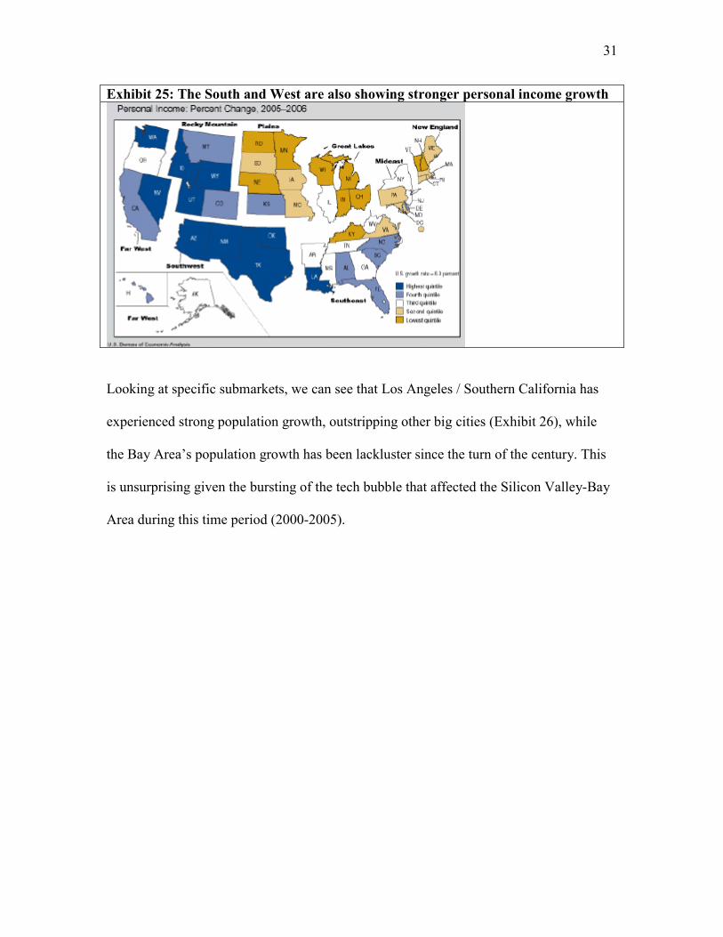
second, respectively, in 2030.” Exhibit 25 shows personal income growth is also stronger
in the South and Western United States. We note that both California and Texas benefit
from these strong population and income trends creating a favorable demand
environment for residential housing.
Exhibit 23: Absolute change in population Population growth is strongest in South and West
Exhibit 24: Percentage change population
31
Exhibit 25: The South and West are also showing stronger personal income growth
Looking at specific submarkets, we can see that Los Angeles / Southern California has
experienced strong population growth, outstripping other big cities (Exhibit 26), while
the Bay Area’s population growth has been lackluster since the turn of the century. This
is unsurprising given the bursting of the tech bubble that affected the Silicon Valley-Bay
Area during this time period (2000-2005).

32
Exhibit 26: Population growth has been strong in Southern California (SCAG) and Dallas; Weak in the San Francisco Bay Area
Southern California has also seen good growth in employment (Exhibit 27), outstripping
both state and national averages. While the Bay Area’s population growth has been
lackluster, the demand story remains very good, driven by strong income growth. Exhibit
28 shows that San Francisco’s average income is well above other major cities and
growth in per capita income is well above the national average (Exhibit 33). As US
income has grown in the post-WWII era, the Bay Area, famous for spawning much of the
American information technology industry in its Silicon Valley, has garnered more than
its share of economic growth. Overall, Southern California ranks poorly on average
income, however there are pockets of affluence in the region as shown in Exhibit 29.

33
Exhibit 27: Southern California has shown above average employment growth
Exhibit 28: San Francisco has higher average income Exhibit 29: Southern California has pockets of affluence
In their “Superstar Cities” report for the National Bureau of Economic Research,
Gyourko, Mayer and Sinai show that San Francisco continues to get richer: high income
groups accounted for less than 20% of the population in 1960 but now account for 50%
(Exhibit 30).

34
Exhibit 30: Evolution of Income Distribution in San Francisco 1950-2000 (in 2000 constant $): San Francisco is getting wealthier
Source: Gyourko/Mayer/Sinai, “Superstar Cities,” NBER #12355, July 2006.
Bay Area productivity has consistently grown faster than other US metropolitan regions,
even through the downturn in the early part of this decade (see Exhibit 31). Corporate
formation through venture activities in high tech and biotech are a key factor in this
wealth creation. The Bay Area receives a disproportionate share of venture funding
(Exhibit 32) in both good and bad years (venture capital’s volatility contributes volatility
to the region’s economy).
Given the uniqueness of the Bay Area for attracting entrepreneurs and perpetuating
technological innovations, we think strong income trends are sustainable and ultimately
support the housing market. With limited supply along the coast, increased demand for

35
housing will have to be satisfied by expansion in land, creating a favorable investment
opportunity.
Exhibit 31: Productivity in the Bay Area has surged, driving income growth and offsetting weak population growth.
Exhibit 32: Bay Area is a magnet for VC funding
Not surprisingly, these dynamics have driven strong per-capita income growth (Exhibit
33) in the Bay Area, helping offset sluggish population growth. Los Angeles per-capita
income continues to grow faster than the national average, this combined with population
growth, makes a compelling demand story in Los Angeles. Dallas has seen strong
population growth, but lower per-capita income growth.

36
Exhibit 33: Per Capita Income Growth has been strong in the Bay Area, while Total Income Growth has been strong in Dallas and Los Angeles.
2002 2003 2004 2005 2002 2003 2004 2005Metropolitan portion of the US 1.8 3.1 6.0 5.0 0.6 2.0 4.9 4.0Los Angeles-Long Beach-Santa Ana, CA 2.4 3.4 6.3 5.1 1.3 2.4 5.6 4.9San Francisco-Oakland-Fremont, CA -3.2 1.1 5.4 5.6 -2.9 1.3 5.6 5.5Dallas-Fort Worth-Arlington, TX 0.7 2.1 6.1 6.7 -1.5 0.1 4.1 4.4
Per capita personal incomePersonal income percent change
Where have prices started to correct?
We are looking for markets where housing prices have started to correct so that we are
not pricing our collateral, the entitled land, at peak market valuations. Evidence from
homebuilders suggests that residential real estate prices in Northern and Southern
California have started to correct.
“The largest concentration [of land associated write-downs] was in the southeast, almost
entirely in Florida, and California, primarily in the more expensive southern Coastal
area.” – Hovnanian earnings call.
“Northern California and Washington D.C, markets that corrected earlier than most,
experienced year-over-year sales gains for the quarter.” – Centex earnings call
“In Sacramento, sales were up 65%. In the Bay Area, sales were up 90%. In our DC-
Metro division, sales were up 10%. So as we said last quarter, there are some markets,
especially those that started into the downturn earliest, that appear to be finding stability.”
– Centex earnings call.
“After peaking in Fall 2005, Southern California’s housing market was flat during 2006,
moving painfully towards a more balanced market.” - LAEDC Economic Forecast 2/07
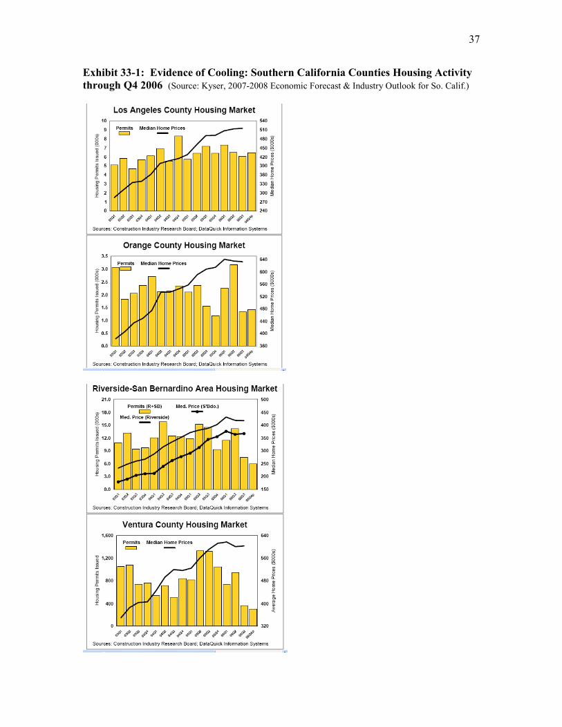
37
Exhibit 33-1: Evidence of Cooling: Southern California Counties Housing Activity through Q4 2006 (Source: Kyser, 2007-2008 Economic Forecast & Industry Outlook for So. Calif.)

38
Risks
We view Los Angeles and the San Francisco Bay Area as attractive markets for our
investment with positive demand factors and constrained supply. The biggest risk factor
we see is housing affordability, which could ultimately impact demand. Housing
affordability in the Los Angeles area is hitting multi-year lows not seen since the late
1980s (Exhibit 34). In addition, a lot of population growth comes from low-income
immigrants, leading to low average household income. The story is similar in the Bay
Area, where housing prices have grown much more rapidly that income (Exhibit 35).
However, we note that affordability has long been a question in both the Los Angeles and
Bay Area housing markets, but home prices have continued to appreciate. We think this
is likely to continue and view them as attractive markets for the financing transaction that
we propose. We note that in contrast, affordability in Dallas remains very good (refer to
Appendix Exhibit 3) due to lower home prices.
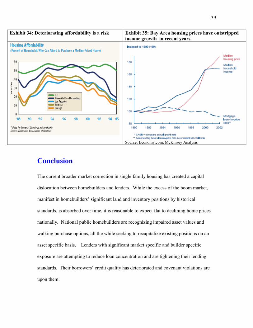
39
Exhibit 34: Deteriorating affordability is a risk Exhibit 35: Bay Area housing prices have outstripped income growth in recent years
Source: Economy.com, McKinsey Analysis
Conclusion
The current broader market correction in single family housing has created a capital
dislocation between homebuilders and lenders. While the excess of the boom market,
manifest in homebuilders’ significant land and inventory positions by historical
standards, is absorbed over time, it is reasonable to expect flat to declining home prices
nationally. National public homebuilders are recognizing impaired asset values and
walking purchase options, all the while seeking to recapitalize existing positions on an
asset specific basis. Lenders with significant market specific and builder specific
exposure are attempting to reduce loan concentration and are tightening their lending
standards. Their borrowers’ credit quality has deteriorated and covenant violations are
upon them.

40
Yet as in most correcting markets we find that popular opinion tends to over-generalize,
and certain resilient assets become caught up in the frenzy. We believe our proposed
transaction addresses the aforementioned needs and recapitalizes mis-priced, high quality
assets in an attractive risk-adjusted structure. In doing so we earn double digit returns
and positive NPV given a debt-like cost of capital. We have carefully underwritten
specific submarkets that do and do not lend themselves to our structure based on supply
and demand fundamentals, and provided a downside scenario whereby we are forced to
foreclose on the assets and carry a substantial burden for several years. We still manage
to earn a nicely positive return that approaches our cost of capital.
In summary, we believe we have derived an efficient way to make a contrarian play in a
correcting market based on sound underwriting and rigorous analysis. While market
conditions today have created this opportunity, we recognize that our proposed structure
is not inherently sustainable over time. Homebuilders will again be flush with capital and
lenders will again be comfortable with the housing sector. However, as long as there are
boom and bust periods in cyclical industries like homebuilding, there will be
opportunities like this to exploit capital markets inefficiency.

41
Bibliography Housing, Regulation & California � Calif. Asso. of Realtors, California Economic Profile, Dec. 2006. � Davidoff, Thomas, “A House Price Is not a Home Price: Land, Structures, and the
Macroeconomy,” UC Berkeley: Haas School of Business, Dec. 18, 2005. � Davis, Morris A. and Heathcote, Jonathan, “The Price and Quantity of Residential Land
in the United States,” Federal Reserve Board of Governors, Washington DC, July 2004. � Davis, Morris A. and Heathcote, Jonathan, “Housing and the Business Cycle,” Federal
Reserve Board of Governors, Washington DC. � Davis, Morris A. and Palumbo, Michael G., “The Price of Residential Land in Large US
Cities,” Federal Reserve Board, Finance & Economics Discussion Series, Washington DC 2006-25.
� Glaeser, Edward and Gyourko, Joseph, “The Impact of Zoning on Housing Affordability,” Cambridge, MA: Harvard Institute of Economic Research, March 2002.
� Glaeser, Edward; Gyourko, Joseph and Saks, Raven, “Why Have Housing Prices Gone Up?,” Cambridge MA: NBER Working Paper 11129, Feb. 2005.
� Glaeser, Edward and Gyourko, Joseph, “Zoning’s Steep Price,” Regulation, Fall 2002. � Glaeser, Edward and Saiz, Albert, “The Rise of the Skilled City,” Cambridge MA: NBER
Working Paper 10191, Dec. 2003. � Glickfeld, Madelyn and Levine, Ned, "Regional Growth and Local Reaction: The
Enactment and Effects of Local Growth Control and Management Measures in California", Cambridge MA: Lincoln Institute of Land Policy, 1992.
� Gyourko, Joseph; Mayer, Christopher and Sinai, Todd, “Superstar Cities,” Cambridge MA: NBER Working Paper 12355, July 2006.
� Gyourko, Joseph and Saiz, Albert, “Is There a Supply Side to Urban Revival?,” Univ. of Pennsylvania, The Wharton School, April 5, 2004.
� Gyourko, Joseph; Saiz, Albert and Summers, Anita, “A New Measure of the Local Regulatory Environment for Housing Markets: The Wharton Residential Land Use Regulatory Index,” Univ. of Pennsylvania, The Wharton School, Oct. 22, 2006.
� Levine, Ned, “The Effects of Local Growth Controls on Regional Housing Production and Population Redistribution in California,” Urban Studies, Vol. 36, No. 12, 1999, p. 2047-2068.
� McAfee, Jamie, “The Rising Costs of Development,” Multifamilty Trends, Jan/Feb. 2007. � Pendall, Rolf; Puentes, Robert and Martin, Jonathan, “From Traditional to Reformed: A
Review of the Land Use Regulations in the Nation’s 50 largest Metropolitan Regions,” Metropolitan Policy Program of The Brookings Institution, Washington DC, Aug. 2006.
� Pollakowski, Henry and Wachter, Susan, “The Effects of Land-Use Constraints on Housing Prices,” Land Economics, Vol. 66, No. 3, Aug. 1990, p. 315-324.
� Porter, Michael E., “The US Homebuilding Industry and The Competitive Position of Large Builders,” Centex Investor Conference, NY, Nov. 18, 2003.
� Property & Portfolio Research, “Land as an Investment Class: Was Will Rogers on to Something?,” Real Estate / Portfolio Strategist, Vol. 10, No. 5, Oct. 2006.
� Property & Portfolio Research, “The End of the Housing Party,” Real Estate / Portfolio Strategist, Vol. 10, No. 4, July 2006.
� Quigley, John and Raphael, Steven, “Regulation and the High Cost of Housing in California,” American Economics Association, Vol. 95, No. 2, May 2005, p. 323-328.
� ULI/Pricewaterhouse Coopers LLP, “Emerging Trends in Real Estate,” 2006 (Oct. 2005) and 2007 (Oct. 2006).

42
Southern California Economy � Girion, Lisa, UCLA Analysts Back Forecast of ‘Soft Landing,’” Los Angeles Times,
Dec. 7, 2006. � Kleinhenz, Robert A., “Housing Affordability in Southern California” (presented at
SCAG Housing Summit), Calif. Asso. of Realtors, April 21, 2005. � Klowden, Kevin and Wong, Perry. “Los Angeles Economy Project.” Milken Institute,
Oct. 2005. � Carreras, Joseph, “Housing Production and Demand Issues in Southern California, Dec.
3, 2003 � Kyser, Jack, et.al., “2007-2008 Economic Forecast & Industry Outlook,” LAEDC, Feb.
2007. � Kyser, Jack, “Westside Economic Update,” LAEDC, 4 Nov. 2005. � LAEDC, “Downtown Los Angeles – 2004 Economic Overview & Forecast,” Feb. 2004. � LAEDC, “Economic Vitality in Changing Times – Westside 2006 Economic Overview &
Forecast,” Nov. 2005. � Los Angeles Downtown Center Business Improvement District, “The Downtown Los
Angeles Market Report & Demographic Survey of New Downtown Residents,” Jan. 2005.
� Southern California Association of Governments. “Housing Element Compliance and Building Permit Issuance in the SCAG Region.” April 2005.
� Southern California Association of Governments. “Housing in Southern California: A Decade in Review.” Jan. 2001.
� Southern California Association of Governments. “Regional Economic Forecast for Southern California 2006-07.” Jan. 26, 2006.
� Southern California Association of Governments. “State of the Region 2006.” Dec. 14, 2006.
Bay Area Economy � Bay Area Economic Forum, “The Future of Bay Area Jobs: The Impact of Offshoring
and Other Key Trends.” Aug. 2004. � Bay Area Economic Profile, “The Innovation Economy: Protecting the Talent
Advantage.” Bay Area Economic Forum, Feb. 2006. � Bay Area Economic Profile, “Downturn and Recovery: Restoring Prosperity.” Bay Area
Economic Forum, Jan. 2004. � Bay Area Council, “Bay Area Housing Profile 2006.” June 30, 2006. � The Forum Reports, “Housing and the Economy.” Vol 2, Number 1. Bay Area Economic
Forum, Winter 1999-2000. � The Forum Reports, “Managing Growth: Regional issues, regional answers?” Vol 2,
Number 2. Bay Area Economic Forum, Summer 2000. Dallas Economy � Aleman, Eugenio, “Texas Outlook,” Wells Fargo Economics, Feb. 2007. � Gaines, James P., “THAI Revised Texas Housing Affordability Index,” Real Estate
Center, Texas A&M University, Oct. 2005. � Greater Dallas Chamber, “Dallas/Fort Worth Metroplex Regional Profile,” 2006. � Greater Dallas Chamber, “DFW Facts,” 2007. � Greater Dallas Chamber, “DFW 101,” Jan. 2007. � Real Estate Center, “Real Estate Market Overview 2006: Dallas-Fort Worth-Arlington,”
Texas A&M University.

43
Appendix Appendix Exhibit 1: Total Expected Unleveraged Returns in 2006, by Real Estate Asset Class
Drawn from: PPR, “Land as an Investment Class,” Oct. 2006, p. 12. Survey data from mid/late 2005. Appendix Exhibit 2: Value/Cost Ratio by US Region and Year
Source: Gyourko/Saiz, “Is There a Supply Side to Urban Revival?,” Wharton.

44
Appendix Exhibit 3: Dallas Affordability
Source: The Real Estate Center, Texas A&M, Oct. 2005