resiliency assessment in distribution networks using gis ... · and historical management data of...
TRANSCRIPT
1
Abstract— A new predictive risk-based framework is proposed
to increase power distribution network resiliency by improving
operator understanding of the status of the grid. This paper
expresses the risk assessment as the correlation between
likelihood and impact. The likelihood is derived from the
combination of Naive Bayes learning and Jenks natural breaks
classifier. The analytics included in a GIS platform fuse together
a massive amount of data from outage recordings and weather
historical databases in just one semantic parameter known as
failure probability. The financial impact is determined by a time
series-based formulation that supports spatiotemporal data from
fault management events and customer interruption cost. Results
offer prediction of hourly risk levels and monthly accumulated
risk for each feeder section of a distribution network allowing for
timely tracking of the operating condition.
Index Terms—Power distribution system, risk assessment,
Naive Bayes learning, failure probability, time series,
interruption cost, geographic information system (GIS).
I. INTRODUCTION
HE proposed predictive risk management framework leads
to proactive risk management and effective ranking of risk
reduction measures [1]. The weather-based risk assessment
provides the spatiotemporal correlation between weather data
and historical management data of the power distribution
system. Historically, the risk assessment was mainly studied in
power transmission system, [2]. The most recent literature on
power distribution system has also focused on risk studies as a
central theme [3]-[9].
In [3], historic reliability data reflecting the variation of
service continuity indices is utilized to develop probability
distribution functions used to illustrate the potential financial
risk associated with assigned reward/penalty structure
integrated in a performance-based regulation plan for
distribution utilities. The histograms of indices, such as system
average interruption frequency index (SAIFI) and duration
This work was fully supported by the FAPESP (grant: 2015/17757-2),
CAPES and CNPq (grant: 305371/2012-6) allowing Dr. Boas Leite to spend a
year with Dr. Kezunovic’s team at Texas A&M University. J. B. Leite and J. R. S. Mantovani are with the Electrical Engineering
Department, UNESP/FEIS, Ilha Solteira, São Paulo, BRAZIL (e-mail:
[email protected], [email protected]). T. Dokic, Q. Yan, P.-C. Chen and M. Kezunovic are with the Department
of Electrical and Computer Engineering at Texas A&M University, College
Station, TX, USA (e-mail: [email protected], [email protected], [email protected], [email protected]).
index (SAIDI), overlap a predefined function that reproduces
the reward/penalty regulation policy, predicting the future
risks. Instead of evaluating the financial risk, [4] introduces a
risk assessment approach that ensures the human safety in
power distribution network by determining the intensity of
fault current levels that are dangerous for people when
stepping on downed conductor and touching poles in a faulted
network. The risk analysis employs the Monte Carlo
simulation using assumptions of probability distribution
functions in the soil resistivity, human body resistance and
heart current. Another study presented in [5] analyzes the risk
from vaults in the underground power distribution system that
can provoke human injuries, monetary compensation, energy
unavailability and traffic disruption on streets.
In [6], the correlation between day-ahead and real-time
markets is integrated in a reliability and price risk assessment
using an energy and pre-dispatch model. Going beyond the
short-term market operation, work in [7] investigates the risk-
based security of concentrated solar power for mid- and long-
term planning horizons. The impact indices are aimed at
minimizing steady-state voltage profile variation, assessing the
line overload security, and verifying the static and dynamic
voltage stability. Similarly, [8] assesses the impact of
increasing the wind power injection into medium-voltage
networks. Investment alternatives taking into account
photovoltaic generation, electric vehicles and other new
technologies at low-voltage network have been assessed by
using the planning framework which determines the risks
based on availability, losses and power quality [9].
Indeed, the risk assessment approach is a wide concept used
in distribution system reliability, security and planning studies.
The recent interest of academia and electricity industry is
encouraging the resilient design of power networks [10] and
resilient operating response [11]. Both approaches require the
resilience evaluation that does not have a defined metric. The
risk assessment is efficiently applied to serve this purpose.
We have proposed several innovative solutions: a)
integration of outage records, historical weather information
and fault management events in a risk-based GIS driven
proactive management tool; b) implementation of a risk model
based on Naive Bayes learning, and classifying the calculated
likelihood using Jenks natural breaks where the financial
impacts are modeled using the time series-based
spatiotemporal formulation, and c) operator visualization of
hourly risk prediction using GIS interface.
Resiliency Assessment in Distribution Networks
Using GIS Based Predictive Risk Analytics
Jonatas Boas Leite, Member, IEEE, José Roberto Sanches Mantovani, Member, IEEE, Tatjana Dokic,
Student Member, IEEE, Qin Yan, Student Member, IEEE, Po-Chen Chen, Student Member, IEEE, and
Mladen Kezunovic, Life Fellow, IEEE
T

2
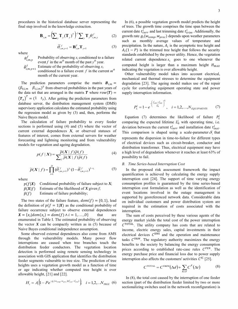
TABLE I. OBSERVED EXTERNAL DEPENDENCES IN THE BAYES MODEL.
xi Feature of interest xi Feature of interest
x1 Wind speed is low x6 Weather is rainy
x2 Wind speed is medium x7 Weather is thunderstorm
x3 Wind speed is high x8 Incidence of lightning x4 Weather is good x9 Vegetation is over height
x5 Weather is misty x10 Degradation by ageing
This paper is organized as follows. Section II specifies the
context that connects the proposed risk assessment framework
to the improvement of the power grid resilience. In the Section
III, the risk matrix mapping is described through the
calculation of failure probability and interruption cost. The
risk matrix is then achieved by using Jenks natural breaks
algorithm for determining risk matrix row/column classes. In
Section IV, explained concepts involving the proposed risk
assessment framework are utilized in the evaluation of a real
world distribution network. The conclusions are given in
Section V before the references at the end.
II. WHERE THE RISK ANALYTICS MEETS THE RESILIENCE
One of the formal definitions of resilience refers to “the
ability of an object to return to its original position after being
stressed. In the power system, it generally refers to the ability
of anticipating extraordinary and high-impact, low probability
events, rapidly recovering and adapts as whole for preventing,
or mitigating, similar events in the future” [12]. In addition
“Because the power grid cannot be totally secure, grid
resilience strategies must identify the greatest risk to the
system and determine the cost and impact to the mitigation
strategies for advancing the capacity of the power grid” [13].
It is also noted that “Replacing, upgrading or making all the
power system components more robust to cope with the
potentially increased impact of severe weather events is a very
expensive and rather unrealistic solution” [14].
In response to the mentioned resilience definition and
proposed mitigation, we offer two developments. One entails
new means of increasing operator situational awareness
through risk-based analysis of the impacts of operator actions
leading to prioritizing mitigation strategies for achieving the
improved grid resilience. The other includes broad set of
preventive actions that can be taken to improve the
observability, controllability, and operational flexibility of a
power system, particularly in response to severe weather
events. Combining the two developments, we achieve the
outcomes that lead to improved resilience. One is a user-
friendly visualization tool using color contours, animated
arrows, dynamic sized pie charts, and three-dimensional
representation of power system leading to better assessment
of the risk during emergencies. The other is a more focused
decision-making tool that offers the predictive assessment of
evolving conditions during severe weather events leading to
preventive mitigation strategies to reduce the risks.
The obtained risk level is a metric in response to
unfavorable event affecting the distribution system. As
defined in the risk analysis theory, the risk assessment is
computed before and after a control action to preserve the
distribution network operating in normal state. This metric
also takes into account all power outages, which enables the
risk assessment for the resiliency evaluation as is defined in
[15] where main differences between resiliency and reliability
are enumerated.
III. RISK MATRIX MAPPING
The measured risk is given by the correlation between the
likelihood of event occurrence along time and consequent
impacts of each event [16]. This correlation is typically
obtained by a risk matrix where the risk is ranked in three
levels: the high level (H) is considered unacceptable risk; the
medium level (M) is dealt as either undesirable or as acceptable
with review; and the low level (L) is treated as acceptable
without review. The number of rows and columns of the risk
matrix is defined by likelihood and impact categories using
Naive Bayes and interruption cost models, respectively.
A. Failure Probability Metric by Naive Bayes Model
The proposed risk assessment framework employs the failure
probability metric to determine the likelihood of something is
malfunctioning in a distribution network. The processing of
large volume of data from diverse databases, i.e. outage
management system (OMS), lightning detection network, GIS,
weather stations, and asset management system (AMS)
database contributes to threats characterization, [17] and [18].
The use of the big data analytics is thus required where the
machine learning technique demonstrates great efficiency in
the knowledge extraction. The Naive Bayes is the supervised
learning technique used to establish an association of several
features of interest into just one quantitative parameter [19].
The knowledge extraction is a function of data mining or
knowledge discovery from data (KDD) that sequentially
groups several functions for dealing with massive database
difficulties, e.g. unnecessary information and inconsistent data
[20]. In this way, the data cleaning, integration and selection
functions are performed before the Naive Bayes model that
processes the useful information. Equation (1) expresses the
conditional probability of failure subjected to observe the
external dependence ix .
f
ii
ifinpoints dataofnumber
fforxtimesnumberfxp
1)|1( (1)
Table I enumerates all external dependences that are given
by different types of threats as features of interest in power
distribution system. In addition, the Naive Bayes conditional
independence assumption among features of interest also
allows to define f
iifxp 1)|0( . The probabilities
achieved by the maximum likelihood learning are average
values from the data set. Since the power distribution system
operating conditions depend on seasonality, the data set is
grouped by years and months. The prediction of the probability
value in the current year and month of analysis is achieved
using a regression model resulting of the ordinary least square
(OLS) estimator, as given by (2) and (3). The elements of mi,Β
are prediction parameters obtained through the stored
3
procedures in the historical database server representing the
final step involved in the knowledge extraction.
y
f
ymiyy
T
yymi ,,
1
, )( ΤΤΤΒ (2)
1,1,,
~ y
T
mi
f
ymi ΤΒ (3)
where
Probability of observing xi conditioned to a failure
event f in the mth month of the past y
th year.
Estimate of the probability of observing xi
conditioned to a failure event f in the current mth
month of the current year.
The prediction parameters comprise the matrix from observed probabilities in the past years of
the data set that are arranged in the matrix where
. After getting the prediction parameters from
database server, the distribution management system (DMS)
supervisory application calculates the estimated probability using
the regression model as given by (3) and, then, performs the
Naive Bayes model.
The calculation of failure probability to every feeder
sections is performed using (4) and (5) where the vector of
current external dependences X, or observed statuses of
features of interest, comes from external servers for weather
forecasting and lightning monitoring and from vulnerability
models for vegetation and ageing degradation.
ffpfp
fpfpfp
)(~)|(~)(~)|(~
)|(X
XX (4)
D
i
xf
ymi
xf
ymiiifp
1
1
1,,1,, )~
1()~
()|(~ X (5)
where
Conditional probability of failure subject to X;
Estimate of the likelihood of X given f;
Estimate of failure probability;
The two states of the failure feature, , lead
the definition of as the conditional probability of
failure occurrence subject to observe external dependences
that are
enumerated in Table I. The estimated probability of observing
the vector X can be compactly written as in (5) because of
Naive Bayes conditional independence assumption.
Some observed external dependences also come from AMS
through the vulnerability models. Many power flow
interruptions are caused when tree branches touch the
distribution feeder conductors. The vegetation location
detection is performed using remote sensing technology in
association with GIS application that identifies the distribution
feeder segments vulnerable to tree size. The prediction of tree
heights uses a vegetation growth model as a function of time
or age indicating whether computed tree height is over
allowable height, [21] and [22].
TREE
ttwwg
ii NiPeAHitrim
icurrprectempi ,...2,1,1
))(,(
(6)
In (6), a possible vegetation growth model predicts the height
of trees. The growth time comprises the time span between the
current date and last trimming date
. Additionally, the
growth rate depends upon weather parameters
such as monthly average values of temperature and
precipitation. In the nature, is the asymptotic tree height and
is the trimmed tree height that follows the security
standards established by the power utility. Hence, the vegetation
related current dependence9
x goes to one whenever the
computed height is larger than a maximum height
indicating the vegetation is over allowable height.
Other vulnerability model takes into account electrical,
mechanical and thermal stresses to determine the equipment
degradation [23]. The ageing model makes use of the repair
cycle for correlating equipment operating state and power
supply interruption information.
EQUIPMENTS
L
tt
i
L NieP
i
i
iinst
icurr
,...,2,1,1 0
(7)
Equation (7) determines the likelihood of failure
comparing the expected lifetime with operating time, i.e.
deviation between the current and installation date
.
This comparison is shaped using a scale-parameteri that
represents the dispersion in time-to-failure for different types
of electrical devices such as circuit-breaker, conductor and
distribution transformer. Thus, electrical equipment may have
a high level of degradation whenever it reaches at least 63% of
possibility to fail.
B. Time Series-based Interruption Cost
In the proposed risk assessment framework the impact
quantification is achieved by calculating the energy supply
interruption cost [24]. The support of time varying energy
consumption profiles is guaranteed by the time series-based
interruption cost formulation as well as the identification of
event locations involved in the outage management is
supported by georeferenced network data. Considerable data
on individual customers and power distribution system are
required in the estimation of costs associated with the
interruption.
The sum of costs perceived by these various agents of the
energy market yields the total cost of the power interruption
. The utility company has costs that are related to
income, electric energy sales, capital investments in their
electrical devices and the operation and maintenance
tasks . The regulatory authority maximizes the energy
benefits to the society by balancing the energy consumption
prices according to established rate-case rules . The
energy purchase price and financial loss due to power supply
interruption also affects the customers' activities [25].
tCdCCK
K
Γ
M&OTOTAL (8)
In (8), the total cost caused by the interruption of one feeder
section (part of the distribution feeder limited by two or more
sectionalizing switches used in the network reconfiguration) is

4
given in two parts. The first part is the operation and
maintenance cost that depends on the route traveled by the
field crew where the distribution network topology,
georeferenced position of sectionalizing switches, initial
position of field crews and GIS routing application are
employed as input information for solving the crew dispatch
problem [26]. The second part is the sum of cost related to
different market agents that are grouped in a set comprising, respectively, the billing loss of
utility company, the penalty cost from regulatory authority
rules, and the economic losses of different types of customers.
These different costs depend on the interruption time ,
i.e. the time span including outage report time (wait time from
the fault occurrence until the dispatch of field crews),
maneuver time (interval involving the field crew travel, feeder
inspection and manual switching to isolate the faulted feeder
section and to restore the adjacent feeder sections) and repair
time (required time to repair the damage equipment and to
restore the energy supply service). Since fault management
procedures change the state of energy customers, the
interruption time is discretized by a pre-defined time step
yielding the set of time series .
Ω Φi j
ji
K
ji
K zctC ,, (9)
In (9), is a binary variable that reproduces state changes
of the jth
customer during the interruption time where the logic
value 1 indicates the interruption in the energy supply. The
set contains all customers on the feeder and the effect of
different market agents over the individual customer cost
as in the following the formulation.
Θ Τm n
nmjnmij
e
jji wFLcc ,,
dem
,,
ENS
, (10)
Additionally to operation and maintenance cost, the utility
company also perceives the billing loss, i.e. the cost of energy
that could be sold to customers during the interruption, given
by the cost of energy not supplied as in (10), where
is
electricity rate and is the installed power of the jth
customer.
The most typical customer types are grouped in while their
consumption profiles are in . In this
way, is a tridimensional data array with load percentage
demand hour-by-hour [24] and, consequently, is a two-
dimensional binary array for indicating the type and
consumption profile of the jth
customer.
ens
,
maxPEN
, , jiji cttiHc (11)
According to the rules established by regulatory authorities
for compensating customers over long outages [27], utility
companies could be penalized and customer compensated
whenever the outage interval exceeds the established limit. In
(11), the penalty cost is determined using the function
that has zero value while the product of is less than the
maximum outage duration . Otherwise, the billing loss
of jth
customer is multiplied by a factor of penalty.
Θ Τm n
nmjnmimimijji wFccLc ,,
dem
,,
CDF
,1
CDF
,
IC
, (12)
The most significant part of the total cost is the customer
interruption cost that associates the economic losses of
different customers during the power supply failures [28].
Wages paid to idle workers, loss of sales, overtime costs,
damage to equipment, spoilage of perishables, cost of running
back-up generators and cost of any special business
procedures contribute to the determination of the customer
interruption cost [29]. In particular, the endangered well-
being, spoiled food and damaged appliances may affect
residential customers. The impact of power interruption is
popular and directly formulated using the customer damage
function by expressing the customer interruption cost as a
function of outage duration [30]. Equation (12) determines the
customer interruption cost for j
th customer in the i
th time
step. The values of time series are interpolations from the
table containing values of customer damage functions that are
typically defined for each economic activity or customer type.
C. Method for Defining the Risk Matrix
The calculation of failure probability and interruption cost
quantifies the likelihood and impact, respectively, and is
performed hour-by-hour for timely risk assessment using the
proposed risk matrix. Hourly values of likelihood and impact
are classified into categories and mapped to rows and columns
of the risk matrix whose elements determine risk levels. Since
levels and categories represent ranges of continuous values, a
clustering methodology is needed to classify the estimated
likelihood, impact and risk, as in Fig. 1.
The Jenks natural breaks algorithm is a common method in
GIS applications able to divide a dataset into a predefined
number of homogeneous classes. This method was originally
introduced as "optimal data classification" because it
minimizes the variance within classes by maximizing the
variance between classes [31]. One-dimensional values that
are not uniformly distributed, as estimated likelihood, impact
and risk, are appropriate for Natural breaks classification [32].
The goodness of variance fit (GVF) is a quality index used
by the Jenks algorithm as stopping criteria. The perfect fit, or
“optimum data classification”, is achieved when .
The Algorithm 1 describes methodically all steps in the Jenks
optimization to obtain the class boundaries with the maximal
similarity from an input dataset U. At the beginning, the class
boundaries are defined by intervals with the same size. Then,
the algorithm adjusts the boundaries systematically until the
Fig. 1. Jenks natural breaks optimization on risk assessment framework.

5
Algorithm 1 Jenks Natural Breaks algorithm.
1: Select the input dataset U to be classified and specify the number of
classes, NC.
2: Define the classes’ boundaries: [INFj, SUPj] to j = 1, 2, …NC, where every interval has the same size.
3: Calculate the sum of squared deviation of the dataset SDU by (13):
UiU uuuSD i ,2 (13)
4: While the GVF is lower than maximum value do 5: Calculate the sum of squared deviation for each class SDj by (14):
jjji,jji SUP,INFuuuSD ,2
,j (14)
6: Increase one standard deviation into the interval [INFj,
SUPj] from classes with lowest SDj by decreasing one into the
interval from classes with largest SDj. 7: Calculate the GVF by (15):
USDSDGVF
NC
j
j
1
1 (15)
8: End while
9: Store the classes’ boundaries of input dataset, U.
minimization of the sum of the squared deviation from the
classes, i. e. until the maximization of GVF is achieved.
The Jenks natural breaks optimization performs the
determination of boundaries for each class, i.e. inferior and
superior limits for each likelihood and impact category as well
as for each risk level. In Fig. 1, the input dataset into Jenks
optimizer comes from calculations of failure probability UL
and interruption cost UI. The product of probabilities and costs
becomes one-dimensional risk dataset UR permitting to use
again the Jenks optimizer on risk level classification. The
illustrated process to determine class boundaries can be a
periodic procedure using data collection from last year.
As demonstrated in Fig. 1, the risk is also quantified by
multiplying times and classified in risk levels
using the Jenks natural breaks algorithm. If quantified values
of likelihood and impact from previous year are disposed into
axes of a dispersion chart then each data point
is classified according to its risk level.
Since the m likelihood and n impact categories have inferior
and superior bounds and cover axes of dispersion chart, there
are a number of mxn discrete regions that determine the value
of each element into risk matrix. In other words, rows and
columns of the risk matrix are mapped into axes of the
dispersion chart that has regions with data points of different
risk classification. For example, data points in a particular
region can have medium or high risk level classification.
n)Π(m,
n)Π(m,
k
k
kjk
jHMLj
inmdp
dp
whereirlevel
},,{, max, (16)
The element of the risk matrix is hence determined
using the density formulation as is given in (16) where the
value of i is equal to the risk level ( , or ) with the
maximum calculated density at the region that is
limited by mth
likelihood category and nth
impact category. In
this way, if the number of data points classified as
low risk level, , is preponderant in the region
. In the region with identical values of calculated
densities, the value of the element representing this region into
mapped risk matrix is equal to the highest risk level because
higher risk levels are less frequent than lower risk levels.
The determination of risk matrix elements completes the
inference mechanism of the proposed online risk assessment for
each feeder section of power distribution network. Although
formulated models are very important in the quantification of
likelihood and impact, the central issue in this work relates to
the process of how to classify these quantities, how to build the
risk matrix and how to develop a DMS tool able to efficiently
display the risk levels using a GIS application. Therefore, the
following section comprises both the construction of risk matrix
by determining classes’ boundaries and the verification of the
developed GIS tool for risk assessment.
IV. GIS VISUALIZATION IN THE DMS
The proposed methodology is evaluated under real world
distribution feeder with data available in [33]. Ten
sectionalizing switches limits nine feeder sections in the
evaluated feeder. These feeder sections have multiple laterals
and electrical loads and are also limited by sectionalizing
switches that must operate during the reconfiguration
procedure. In the calculation of failure probability, the
learning information comes from external sources: two
weather stations and one lightning detection network, where
the historical databases comprise seven years, from 2009 to
2015. Parameters of the vegetation growth model are adjusted
by considering the tree pruning schedule equals to one year
whereas the equipment degradation vulnerability model of
different devices may have their parameters obtained using the
method discussed in [23]. In terms of interruption cost, the
input dataset can be found in [24]. Both calculations obtain
quantified values of likelihood and impact for each feeder
section. A general purpose programming language (C++) is
used in the implementation of the proposed models that are
integrated with a distribution network simulation platform for
supporting the use georeferenced data [34].
A. Building the Risk Matrix
The first process comprises the determination of quantified
likelihood ranges by defining inferior and superior boundaries
of rows categories listed in Table II through Jenks
optimization. In the classification process, the histogram was
built using around five thousand values of failure probability.
Fig. 2 shows the histogram of the distribution of failure
probabilities where the frequency axis is rated using
logarithmic scale of base ten. A histogram in linear scale is
shown at the far-right corner, which helps to deduce the
absence of a probability density function able to characterize
the likelihood. There are failure probability values with zero
frequency because the set of external dependences, X, has a
finite number of features of interest and the occurrence
probability for each feature of interest is calculated monthly.
Despite this characteristic, the Jenks optimizer found the six
likelihood categories and their range limits by a GVF index
being equal to 0.98704. For example, the likelihood category
III comprises failure probability values between 0.31 and 0.54.

6
TABLE III. DETERMINED ELEMENTS OF THE RISK MATRIX.
IMPACT
A B C D E F
LIK
EL
IHO
OD
I L L L L L L
II L L L L L M
III L L M M M H
IV L M M M H H
V M M M H H H
VI M M M H H H
TABLE II. ROWS AND COLUMNS CATEGORIES OF THE RISK MATRIX.
Rows Columns
Categories Description Categories Description
LIK
EL
IHO
OD
I Extremely Unlikely
IMP
AC
T
A Insignificant
II Highly Unlikely B Minor
III Doubtful C Significant
IV Very Unlikely D Serious
V Unlikely E Major
VI Likely F Catastrophic
The second process involves the determination of quantified
impact categories in Table II by determining their boundaries.
Fig. 3 displays the histogram of the distribution of interruption
cost values where frequency was obtained by taking into
account a series of intervals each equal to $500. The
distribution characteristic is shown by the histogram in linear
scale helping to deduce that interruption cost values can be
featured by a Weibull probability distribution. Although the
economic activity and consumption profile are important
factors in the cost calculation, the interruption duration, which
also figures the Weibull probability density function, is the
factor with the greatest influence over the interruption cost.
Six impact categories were achieved by Jenks algorithm
with GVF index equals to 0.96149. The first three impact
categories have shorter ranges due to large frequencies in this
region. Consequently, the impact category B has the shortest
range equals to $3,500, whereas the category F comprise the
longest range, from $20,450 to $31,670.
The third process deals with the determination of risk levels
by defining their boundaries. Fig. 4 demonstrates the histogram
of the distribution of quantified risk values using a series of
intervals equal to $500, as well. The linear scale-based
histogram at far-end right corner reveals that risk distribution
has the behavior of an exponential probability distribution, so
the most adequate classification methodology should be
performed by head/tail breaks classifier [35]. In this case, the
Jenks optimizer can be used again because the quantified risk is
grouped in few numbers of classes, i.e. in three risk levels, and
the density method should still determine the preponderant
characteristic for each region at dispersion chart what admits
data points that are classified with less degree of accuracy.
Three risk levels were achieved using the Jenks algorithm
with GVF index equals to 0.83967. Although the quality index
had been worse than GVF indices in quantified likelihood and
impact classification, the achieved risk level ranges fit with
heavy-tailed distribution. For instance, the head risk level, L,
has range equals to $3,200 in contrast to the tail risk level, H,
with range of $21,900.
After the determination of class boundaries, the next
process consists of the construction of risk matrix using the
density method. Table III presents elements of the risk matrix
where rows are likelihood categories and columns are impact
categories. Now, the hourly risk assessment can be executed
using previously determined categories and risk matrix.
B. Study Case under Real Distribution Network
According to the Table III, each risk level is identified by a
color. The GIS application thus assigns for the graphical
representation of the feeder section the color corresponding to
the risk level. Furthermore, the addition of daily hours to set of
spatial coordinates includes one more dimension into feeder
section representation in GIS application. This extra
dimension has the risk level information represented hour-by-
hour, which is well suited to perform online risk mitigation.
Fig. 5 shows a screen shot with the tridimensional graphical
representation of the tested distribution network where
different colors are hourly risk levels. The base of the graphic
corresponds to daily early hours, from 00:00 to 06:00 of
Fig. 4. Distribution of quantified risk values in risk level ranges.
Fig. 3. Distribution of interruption cost values in impact category ranges.
Fig. 2. Distribution of failure probability values in likelihood category ranges.

7
January, 14th of 2016, with low risk level in all feeder
sections. After that, both weather condition and energy
consumption profile are modified causing changes in risk level
of feeder sections. For example, feeder section #1 presents
very low risk level but, along the day, its risk level was
classified as medium because of weather changes. At 20:00,
the observed weather pattern was thunderstorm with medium
wind speed given by causing the
feeder section #2 to change its risk level from medium to high
risk. Although weather changes influence the risk level in
feeder section #3, the main color is intense red representing
the high risk level that is a consequence of economic activities
from customers with large installed power.
The features of interest represented by x8, x9 and x10 are
associated with the lightning, vegetation and ageing respectively,
and have focused behavior associated with each power grid
component whereas the other weather dependences cover a larger
area. As the region of the city under study has many feeder
sections with several power grid components, it becomes
infeasible to represent all the assigned values to these features of
interest when used in the determination of risk levels.
The other way of taking advantage of the developed GIS
tools is in risk management by assigning the value attribution
to risk levels. For instance, low level is equals to 0, medium is
equals to 1 and high is 2. Thus, the different grades of the
accumulated, or continuous sum, risk along the distribution
network are visualized using color temperature scale in
overlapped layers with different accumulated risk values. Fig
6 shows the accumulated risk values during January where the
smaller accumulated risk values are the first layers in cold
color while the larger values are the last layers in hot color.
The feeder section #1 has one lower layer in cold color
indicating the accumulated risk is small. On the other hand,
the feeder section #2 had upper layers with hot color tones
indicating its large accumulated risk, which is the consequence
of customers' types connected in this section.
The high risk level does not just depend on the failure
probability but also on the impact intensity, as is established in
Table III. But the risk level must be either medium (M) or
high (H) whenever the failure probability quantization has
large value and it is classified as Likely (VI). In the
comparison process using records of risk levels, the existence
of low (L) risk level at the past occurrence of a failure event
Fig. 6. Partial screen of the developed GIS application with tridimensional representation of accumulate risk levels during a month.
Fig. 5. Partial screen of the developed GIS application with tridimensional representation of risk levels hour-by-hour.

8
indicates hence a mismatching of the proposed methodology.
Fig. 7 shows that the proposed methodology presents a
mismatching ratio around 20% whenever the cause of failure
event is adverse weather, component failure or lightning.
When the cause is vegetation contact, the ratio improves to
10%. Subsequently, the hours after one mismatching the
correct risk level are calculated and indicated by the proposed
methodology. The bar chart of delayed hours demonstrates
that the delay time does not exceed five hours and in the most
part of mismatching occurrences the correct risk level is
indicated with one hour of delay. These results reveal the
effectiveness of the proposed methodology for evaluating the
jeopardized operating condition of power distribution grids.
V. CONCLUSION
We have shown that the weather-based risk assessment can
provide risk quantification through the correlation involving
available weather data and historical management data of the
power distribution system.
Once the realization of this risk assessment step is
implemented, one can then integrate it with the advanced
distribution management system to offer risk mitigation. This
tool facilitates the operators’ decisions since it employs
spatiotemporal GIS based visualization for the resiliency
improvement actions.
REFERENCES
[1] D. Vose, Risk Analysis: a Quantitative Guide, 3rd ed., vol. 1, West Sussex, England: John Wiley & Sons, 2008, 729 pp.
[2] T. Dokic et al., “Risk Assessment of a Transmission Line Insulation Breakdown due to Lightning and Severe Weather,” in Proc.HICSS, Kauai, HI, 2016, pp. 2488-2497.
[3] R. Billinton and Z. Pan, “Historic Performance-based Distribution System Risk Assessment,” IEEE Trans. Power Del., vol. 19, no. 4, pp. 1759-1765, Oct. 2004.
[4] J. L. Pinto and M. Louro, “On Human Life Risk-Assessment and Sensitive Ground Fault Protection in MV Distribution Networks,” IEEE Trans. Power Del., vol. 25, no. 4, pp. 2319-2327, Oct. 2010.
[5] T. V. Garcez and A. T. de Almeida, “Multidimensional Risk Assessment of Manhole Events as a Decision Tool for Ranking the Vaults of an Underground Electricity Distribution System,” IEEE Trans. Power Del., vol. 29, no. 2, pp. 624-632, Apr. 2014.
[6] Y. Ding, M. Xie, Q. Wu and J. Ostergaard, “Development of Energy and Reserve Pre-Dispatch and Re-Dispatch Models for Real-Time Price Risk and Reliability Assessment,” IET Gener. Transm. Distrib., vol. 8, no. 7, pp. 1338-1345, Jul. 2014.
[7] R. Shah, R. Yan and T. K. Saha, “Chronological Risk Assessment Approach of Distribution System with Concentrated Solar Power Plant,” IET Gener. Transm. Distrib., vol. 9, no. 6, pp. 629-637, Aug. 2015.
[8] W. Deng et al., “Multi-Period Probabilistic-Scenario Risk Assessment of Power System in Wind Power Uncertain Environment,” IET Gener. Transm. Distrib., vol. 10, no. 2, pp. 359-365, Feb. 2016.
[9] M. Nijhuis, M. Gibescu and S. Cobben, “Risk-based Framework for the Planning of Low-Voltage Networks Incorporating Severe Uncertain,” IET Gener. Transm. Distrib., vol. 11, no. 2, pp. 419-426, Jan. 2017.
[10] H. Nagarajan et al., “Optimal Resilient Transmission Grid Design,” in Proc. PSCC, Genoa, Italy, 2016, pp. 1-7.
[11] G. Huang et al., “Integration of Preventive and Emergency Responses for Power Grid Resilience Enhancement,” IEEE Trans. Power Syst., vol. 32, no. 6, pp. 4451-4463, Mar. 2017.
[12] M. Panteli and P. Mancarella, “The grid: stronger, bigger, smarter?: Presenting a conceptual framework of power system resilience,” IEEE Power and Energy Magazine, vol. 13, no. 3, pp. 58–66, Apr. 2015.
[13] Executive Office of the President, “Economic Benefits of Increasing Electric Grid Resilience to Weather Outages,” http://energy.gov/sites/prod/files/2013/08/f2/Grid%20Resiliency%20Report FINAL.pdf, Tech. Rep., Aug. 2013.
[14] M. Panteli and P. Mancarella, “Influence of extreme weather and climate change on the resilience of power systems: Impacts and possible mitigation strategies,” Elect. Power Syst. Res., vol. 127, pp. 259–270, Jun. 2015.
[15] S. Chanda and A. K. Srivastava, “Defining and Enabling Resiliency of Electric Distribution Systems with Multiple Microgrids,” IEEE Trans. Smart Grid, vol. 7, no. 6, pp. 2859-2868, Nov. 2016.
[16] B. M. Ayyub, “Risk Analysis Methods,” in Risk Analysis in Engineering and Economics, 1st ed., vol. 1, Boca Raton, FL: Chapman & Hall/CRC, 2003, pp. 33-118.
[17] P. Chen, T. Dokic and M. Kezunovic, “The Use of Big Data for Outage Management in Distribution System,” in Proc. CIRED, Rome, Italy, 2014, pp. 1-5.
[18] M. Kezunovic, L. Xie and S. Grijalva, “The Role of Big Data in Improving Power System Operation and Protection,” in Proc. IREP, Rethymnon, Greece, 2013, pp. 1-9.
[19] D. Lowd and P. Domingos, “Naive Bayes Models for Probability Estimation,” in Proc. ICML, Bonn, Germany, 2005, pp. 1-8.
[20] J. Han, M. Kamber and J. Pei, Data Mining: Concepts and Techniques, 3rd ed., vol. 1, Waltham, MA: Elsevier Inc., 2012, p. 740.
[21] D. T. Radmer et al., “Predicting Vegetation-Related Failure Rates for Overhead Distribution Feeders,” IEEE Trans. Power Deliv., vol. 17, no. 4, pp. 1170-1175, Oct. 2002.
[22] F. B Martins, C. P. B. Soares and G. F. da Silva, “Individual Tree Growth Models for Eucalyptus in Northern Brazil,” Sci. Agric., vol. 71, no. 3, pp. 212-225, May 2014.
[23] X. Zhang and E. Gockenbach, “Component Reliability Modeling of Distribution Systems based on Evaluation of Failure Statistics,” IEEE Trans. Dielec. & Elect. Insul., vol. 14, no. 5, pp. 1183-1191, Oct. 2007.
[24] J. B. Leite et al., “The Impact of Time Series-Based Interruption Cost on Online Risk Assessment in Distribution Networks,” in Proc. T&D LA, Morelia, Mexico, 2016, pp. 1-6.
[25] M. J. Sullivan et al., “Interruption Costs, Customer Satisfaction and Expectations for Service Reliability,” IEEE Trans. Power Syst., vol. 11, no. 2, May 1996.
[26] P. M. S. Carvalho, F. J. D. Carvalho and L. A. F. M. Ferreira, “Dynamic Restoration of large-Scale Distribution Network Contingencies: Crew Dispatch Assessment,” in Proc. Powertech, Lausanne, Switzerland, 2007, pp. 1453-1457.
[27] C. J. Wallnerstrom and P. Hilber, “Vulnerability Analysis of Power Distribution Systems for Cost-Effective Resource Allocation,” IEEE Trans. Power Syst., vol. 27, no. 1, pp. 224-232, Feb. 2012.
[28] Q. Yan, T. Dokic and M. Kezunovic, “Predicting Impact of Weather Caused Blackouts on Electricity Customers Based on Risk Assessment,” in Proc. PESGM, Boston, MA, 2016, pp. 1-6.
[29] N. Kaur et al., “Evaluation of Customer Interruption Cost for Reliability Planning of Power System in Developing Economies,” in Proc. PMAPS, Ames, IA, 2004, pp. 752-755.
[30] R. Billinton and W. Wangdee, “Approximate Methods for Event-Based Customer Interruption Cost Evaluation,” IEEE Trans. Power Syst., vol. 20, no. 2, pp. 1103-1110, May 2005.
[31] G. F. Jenks, “The Data Model Concept in Statistical Mapping,” in International Yearbook of Cartography, vol. 7, Liverpool, England: George Philip & Son Ltd., 1967, pp. 186-190.
[32] T. Slocum et al., Thematic Cartography and Geovisualization, 3rd ed., vol. 1, Upper Saddle River, NJ: Pearson Prentice Hall, 2009, p. 561.
[33] S. Commission. (2016, Mar.). Distribution testing system of 1807 lines. UNESP, Ilha Solteira, Brazil. [Online]. Available: http://www.feis.unesp.br/Home/departamentos/engenhariaeletrica/lapsee807/home/distribution_network_1806_lines.rar.
[34] J. B. Leite and J. R. S. Mantovani, “Development of a Smart Grid Simulation Environment, Part II: Implementation of the Advanced Distribution Management System,” J. Control Autom. Electr. Syst., vol. 26, no. 1, pp. 96-104, Feb. 2015.
[35] B. Jiang, “Head/Tail Breaks: A New Classification Scheme for Data with a Heavy-Tayled Distribution,” J. Prof. Geogr., vol. 65, no. 3, pp. 482-494, Jul. 2013.
Fig. 7. Comparison of the percentages of risk levels by failure events.

9
VI. BIOGRAPHIES
Jonatas Boas Leite (S’10–M’15) received the B.Sc. and Ph.D. degrees in
electrical engineering from São Paulo State University (UNESP) /Ilha
Solteira, SP, Brazil, in 2010 and 2015, respectively. He was a Post-Doctoral
Researcher in the Electrical and Computer Engineering Department, Texas A&M University/College Station, TX, USA and in the Electrical Engineering
Post-Graduate Program of UNESP/Ilha Solteira, SP, Brazil, in 2016 and 2019,
respectively. He is currently a Professor with the Department of Electrical Engineering, UNESP/Ilha Solteira, SP, Brazil and is joined to LaPSEE
(Laboratorio de Planejamento de Sistemas de Energia Eletrica), Ilha Solteira,
SP, Brazil. His research areas are planning and control of electric power systems.
José Roberto Sanches Mantovani (M’06) received the Electrical Engineer
degree from the São Paulo State University – UNESP, Ilha Solteira – SP, Brazil, in 1981. He received the M.Sc. and Ph.D. degree in electrical
engineering from the University of Campinas, São Paulo, Brazil, in 1987 and
1995, respectively. He is currently a Full Professor with the Department of Electrical Engineering, São Paulo State University, UNESP and is joined to
LaPSEE (Laboratorio de Planejamento de Sistemas de Energia Eletrica) Ilha
Solteira - SP, Brazil. His research interests include the planning and control of electric power systems.
Tatjana Dokic (S’10) received the B.Sc. and M.Sc. degrees in electrical and
computer engineering from the University of Novi Sad, Novi Sad, Serbia, in 2012. She is a graduate student with Texas A&M University, College Station,
TX, USA. Her main research interests include power system asset and outage
management, weather impacts on power systems, big data for power system applications, vegetation management, insulation coordination, and fault
location.
Qin Yan (S’12) received the B.S. degree in electrical engineering from
Wuhan University, China, in 2010 and the M.Eng. degree from Texas A&M University, College Station, in 2012, where she is currently pursuing the Ph.D.
degree. Her research interests include plug-in electric vehicles, smart grid,
distributed energy resources, and optimization algorithms.
Po-Chen Chen (S’12) received the B.Sc. and M.Sc. degrees in electrical
engineering from the Polytechnic Institute of New York University, Brooklyn,
NY, USA, in 2010 and 2012, respectively. He is currently pursuing the Ph.D. degree in electrical engineering with Texas A&M University, College Station,
TX, USA. His areas of interest include distributed generation, power system
analysis, power system protection and control, voltage quality and stability studies, and big data application for distribution system
Mladen Kezunovic (S’77–M’80–SM’85–F’99–LF’17) received the Dipl. Ing.
from University of Sarajevo, Sarajevo, Bosnia, M.Sc. from University of Kansas, Lawrence, KS, and Ph.D. degrees in electrical engineering from
University of Kansas, Lawrence, KS, in 1974, 1977, and 1980, respectively.
He has been with Texas A&M University, College Station, TX, USA, for 31 years, where he is currently a Regents Professor and an Eugene E. Webb
Professor, the Director of the Smart Grid Center, and the Site Director of
“Power Engineering Research Center, PSerc” consortium. He is currently the Principal of XpertPower Associates, a consulting firm specializing in power
systems data analytics. His expertise is in protective relaying, automated
power system disturbance analysis, computational intelligence, data analytics, and smart grids. He has authored over 550 papers, given over 120 seminars,
invited lectures, and short courses, and consulted for over 50 companies
worldwide. Dr. Kezunovic is a CIGRE Fellow and an Honorary Member. He is currently a Registered Professional Engineer in Texas.