Resilient Supplier Selection in Logistics 4.0 with Heterogeneous Information

Md Mahmudul Hasan

Department of Mechanical and Industrial Engineering,

Northeastern University

360 Huntington Ave, Boston, MA 02115, USA

email: hasan.mdm@husky.neu.edu

Dizuo Jiang

Department of Mechanical and Industrial Engineering,

Northeastern University

360 Huntington Ave, Boston, MA 02115, USA

email: jiang.di@husky.neu.edu

A. M. M. Sharif Ullah

School of Regional Innovation and Social Design Engineering,

Kitami Institute of Technology

165 Koen-cho, Kitami, Hokkaido 090-8507, Japan

email: ullah@mail.kitami-it.ac.jp

Corresponding author

Md. Noor-E-Alam*

Department of Mechanical and Industrial Engineering,

Northeastern University

360 Huntington Ave, Boston, MA 02115, USA

*Corresponding author email: mnalam@neu.edu

Abstract: Supplier selection problem has gained extensive attention in the prior studies. However, research

based on Fuzzy Multi-Attribute Decision Making (F-MADM) approach in ranking resilient suppliers in

logistic 4.0 is still in its infancy. Traditional MADM approach fails to address the resilient supplier selection

problem in logistic 4.0 primarily because of the large amount of data concerning some attributes that are

quantitative, yet difficult to process while making decisions. Besides, some qualitative attributes prevalent

in logistic 4.0 entail imprecise perceptual or judgmental decision relevant information, and are substantially

different than those considered in traditional suppler selection problems. This study develops a Decision

Support System (DSS) that will help the decision maker to incorporate and process such imprecise

heterogeneous data in a unified framework to rank a set of resilient suppliers in the logistic 4.0 environment.

The proposed framework induces a triangular fuzzy number from large-scale temporal data using

probability-possibility consistency principle. Large number of non-temporal data presented graphically are

computed by extracting granular information that are imprecise in nature. Fuzzy linguistic variables are

used to map the qualitative attributes. Finally, fuzzy based TOPSIS method is adopted to generate the

ranking score of alternative suppliers. These ranking scores are used as input in a Multi-Choice Goal

Programming (MCGP) model to determine optimal order allocation for respective suppliers. Finally, a

sensitivity analysis assesses how the Supplier’s Cost versus Resilience Index (SCRI) changes when

differential priorities are set for respective cost and resilience attributes.

Keywords: Logistic 4.0, Resilience, Supplier selection, Supplier’s Cost versus Resilience Index (SCRI),

TOPSIS, Fuzzy Multi-Attribute Decision Making (F-MADM)

1. Introduction

With the increasing requirements for industrial process due to technological revolution, companies are

facing rigorous challenges such as competitive global industry, increasing market unpredictability, swelling

customized product demands and shortened product renewal cycle (Hofmann & Rüsch, 2017). Aligned

with the demanding industry, the fourth wave of technological innovation has been materialized, known as

Industry 4.0. It refers to so-called fourth industrial revolution in discrete and

process manufacturing, logistics and supply chain (Logistics 4.0), energy (Energy 4.0) etc., which is

resulted due to the digital transformation of industrial markets (industrial transformation) integrated with

smart manufacturing. Powered by foundational technology such as autonomous robots, simulation, cyber

security, the cloud and additive manufacturing (Rüßmann et al., 2015), Industry 4.0 improves the

manufacturing systems to an intelligent level that takes advantage of advanced information and

manufacturing technologies to achieve flexible, smart, and reconfigurable manufacturing processes in order

to address a dynamic and global market (Zhong, Xu, Klotz, & Newman, 2017).

As an essential and significant part of Industry 4.0, Logistics 4.0 concerns the various aspects of end-to-

end logistics in the context of Industry 4.0, the Internet of Things (IoT), cyber-physical systems,

automation, big data, cloud computing, and Information technology (Hofmann & Rüsch, 2017; i-SCOOP,

2017a; Rüßmann et al., 2015; Zhong et al., 2017). Logistics 4.0 aims to develop a smart logistics system to

fulfill the customer requirements in the current connected, digitalized and rapidly changing global logistics

market (i-SCOOP, 2017b). To adopt with an Industry 4.0 environment, extensive cutting-edge applications

have been landed within logistics 4.0. Juhász and Bányai (2018) identified challenges of just-in-sequence

supply in the automotive industry from the aspect of Industry 4.0 solutions and detected impacts of Industry

4.0 paradigm on just-in-sequence supply. Ivanov, Dolgui, Sokolov, Werner, and Ivanova (2016) proposed

a dynamic model and algorithm for short-term supply chain scheduling problem that simultaneously

considered both machine structure selection and job assignments in smart factories. Brettel, Friederichsen,

Keller, and Rosenberg (2014)visualized the supply chain process by introducing cyber-physical systems to

bridge the advanced communication between machines on the landscape of Industry 4.0.

With higher priority on customer satisfaction, incremental attention has been drawn to the availability,

reliability, flexibility and agility of the logistics system (Barreto, Amaral, & Pereira, 2017; Witkowski,

2017). Unpredictable natural catastrophes or unexpected man-made disasters, such as earthquakes, floods,

labor strikes and bankruptcy engender serious threat to the capability of the logistics system on these

aspects. Despite of low occurrence probability, the tremendous financial impacts of the disruptions in any

form on the logistics system are much more obvious. Renesas Electronics Corporation, a Japanese

semiconductor manufacturer and the world’s largest manufacturer of microcontrollers is an industry 4.0

company. They launched the R-IN32M4-CL2 industrial Ethernet communication specific standard product

(ASSP) with integrated Gigabit PHY to support the increasing network and productivity for Industry 4.0

companies on June 25, 2015 (Corporation, 2015). In earthquake and tsunami that struck the northeast coast

of Japan on March 2011, the corporation’s Naka Factory and other manufacturing facilities were severely

damaged by the earthquake. The total losses caused by the disaster was 814.2 million USD, even though

the insurance covered 198.9 million USD (Ye & Abe, 2012). UPS, the leading logistics company, which

has achieved great advancement in the fields of digitalized logistics system and smart factory in the wave

of Industry 4.0, suffers from the lack of resilient supply chain as well. During the hurricane Florence that

threatened the east coast in mid-September 2018, the delivery rate reduced to 50% with thousands of

delivery exceptions (SUPPLYCHAINDIVE, 2018).

To withstand against disruption a resilient supplier is indispensable in the sourcing decision process while

operating under the principles of logistics 4.0. A resilient supplier usually has high adaptive capability to

reduce the vulnerability against disruptions, absorb disaster impact and quickly recover from disruption to

ensure desired level of continuity in operations following a disaster (Y. Sheffi & Rice Jr, 2005; Y. J. M. P.

B. Sheffi, 2005). To comprehensively evaluate the alternatives and select the optimal supplier, diverse

factors are needed to be taken into consideration. Several proactive strategies such as suppliers’ business

continuity plans, fortification of suppliers, maintaining contract with back up suppliers, single and multiple

sourcing, spot purchasing, collaboration and visibility are considered to enhance supply chain resilience in

the presence of operational and disruption risks (Namdar, Li, Sawhney, & Pradhan, 2018; Torabi,

Baghersad, & Mansouri, 2015). Another study suggests that suppliers’ reliability, and flexibility in

production capacity play key role in developing contingency plans to help mitigate the severity of

disruptions (Kamalahmadi & Mellat-Parast, 2016). Criteria such as supply chain complexity, supplier

resource flexibility, buffer capacity and responsiveness were considered in traditional resilient supplier

selection problem (Haldar, Ray, Banerjee, & Ghosh, 2012, 2014). However, to select the resilient supplier

in logistics 4.0 environment, additional aspects are required to be taken into consideration regarding the

features of logistics 4.0.

In logistics 4.0, most of the companies and related organizations are adopting end-to-end information

sharing technologies because the amount of data produced and shared through the supply chain is

significantly increasing (Domingo Galindo, 2016; G. Wang, Gunasekaran, Ngai, & Papadopoulos, 2016).

Driven by the extensive practical and efficient attributes, numerous applications of big data are employed

in delivery forecasting, optimal routing, and productivity monitoring and labor reduction (Waller &

Fawcett, 2013). Making well-informed decisions in sourcing process also involves a variety of massive

data-based logistics aspects evaluation such as delivery lead time, inventory level, production capacity, and

operational investment. Information sources such as ERP transaction data, GPS-enabled data, machine-

generated data and RFID data are frequently transferred, stored and retrieved through the logistics system,

which require massive data manipulation methodology (Rozados & Tjahjono, 2014).

With the widespread use of IoT, cyber-physical systems, and Information technology, attention has been

given on the supplier’s performance and ability in responding to changing customer demand with agility,

warehouse automation, logistics system digitalization, information management and IT security, etc. The

relevant data from these fields are generally collected in various formats at quick velocity, and entails large

volume—all-together leads to Big Data, which is often available as real-time and historical data. Data that

are collected in real-time is characterized by time series whereas historical data is often presented in

graphical format. Attributes that entail large amount of information in logistics 4.0 are inventory level,

schedule of delivery, production capacity, cost etc. Processing these large amounts of data requires a formal

computation process that can enable decision maker to efficiently evaluate alternative decisions.

Therefore, for selecting resilient suppliers in logistics 4.0, a decision-making framework is needed given

the extensive impact of sourcing decision on the supply chain resiliency, efficiency and sustainability. The

decision problem involves evaluation of several alternative suppliers against multiple conflicting criteria.

Moreover, this problem even becomes more complicated when the decision relevant information (DRI) are

in heterogeneous form such as qualitative information that are imprecise in nature and vague sometimes,

and large number of quantitative information that are difficult to process. To address this problem, we

propose a Decision Support System (DSS) leveraging the principle of Multi-Attribute Decision Making

(MADM) to rank alternative suppliers from resilience and logistic 4.0 perspectives.

The key contributions of this study are:

i. As the existing research on MADM has limited applicability in the logistics 4.0 environment, we,

for the first time extend the F-MADM framework to logistics 4.0 industries where selecting resilient

suppliers has far reaching consequence. The proposed DSS is capable of handling qualitative

attributes that entails imprecise DRI, and are substantially different than those considered in

traditional supplier selection problem. Moreover, our plan is to integrate large number of

quantitative DRI, which in logistics 4.0 environment is characterized by time series and graphical

information. As such, we propose an integrated decision-making framework to process this

heterogeneous information in a seamlessly unified framework to facilitate the resilient supplier

selection process for a logistics 4.0 industry.

ii. Commonly used fuzzy based TOPSIS technique solely depends on the standard triangular linguistic

class to handle the qualitative appraisal in the decision making process and lacks the sophistication

in processing the quantitative information. Our proposed DSS overcomes this limitation by

successfully converting and integrating the crisp granular information extracted from graphically

presented data into triangular fuzzy based TOPSIS decision matrix. Crisp granular or c-granular

information refers to the pieces of information entailing well–defined crisp or ill-defined perceptual

boundary consisting of sharp numbers (Ullah & Noor-E-Alam, 2018; Lotfi A. Zadeh, 1997).

iii. Selecting suppliers by considering all attributes that share equal preference usually generate

inflated set of ranking score which is generic, however, sometimes fails to address the issue if a

decision maker wants to put more importance on one set of criteria than another. We divide the

attributes in two sets—mainly based on measure of resilience and cost—used as efficiency measure.

We further demonstrate the capability of the proposed DSS to generate Supplier’s Cost versus

Resilience Index (SCRI) based on customized preference given by the decision makers on cost and

resilience attributes.

iv. We also extend the proposed DSS with the help of an order allocation model leveraging Multi-

Choice Goal Programming (MCGP) technique. The optimal suppliers identified with the help of F-

MADM approach are only suitable for single-sourcing problems in which the procurement quantity

can be satisfied by a single supplier. However, in a situation where procurement demand cannot be

fulfilled by a single supplier, and strategic decision makers want to diversify their market, stabilize

their sourcing channels while distributing risks on multiple suppliers and drive up competitiveness,

allocating orders among competitive suppliers can turn out to be a viable strategy. As such, our

framework will empower decision makers to allocate orders among alternative suppliers by taking

into account the ranking of individual suppliers that has been generated via F-MADM approach.

The rest of this paper is organized as follows. In Section 2, we review the relevant literatures. Then in

section 3 and 4, we present the theoretical concept needed to design the decision-making framework.

Section 5 describes the proposed DSS for suppler evaluation and order allocation problem. In Section 6,

we illustrate the effectiveness of the proposed DSS via a case study. Finally, in Section 7 we conclude the

work conducted in this study with future research directions.

2. Literature review

Multi-Criteria Decision Analysis (MCDA) approaches are widely adopted in the fields of transportation,

immigration, education, investment, environment, energy, defense and healthcare (Devlin, Sussex, &

Economics, 2011; Dodgson, Spackman, Pearman, & Phillips, 2009; Gregory et al., 2012; Mühlbacher,

Kaczynski, & policy, 2016; Nutt, King, & Phillips, 2010; Wahlster, Goetghebeur, Kriza, Niederländer, &

Kolominsky-Rabas, 2015). Howard and Ralph (Raiffa & Keeney, 1975) first introduce MCDA as a

methodology for evaluating alternatives based on individual preference, often against conflicting criteria,

and combining them into one single appraisal. Prior studies have also applied MCDA approach to select

suppliers using multiple attributes (Lo & Liou, 2018; Ren, Xu, & Wang, 2018; Sodenkamp, Tavana, & Di

Caprio, 2018). Multi-Criteria Decision Making (MCDM) with grey numbers was used to propose a

conceptual framework for suppliers’ management entailing selection, segmentation and development of

resilient suppliers (Valipour Parkouhi, Safaei Ghadikolaei, & Fallah Lajimi, 2019). They used Grey

DEMATEL technique to weigh the criteria considered for the two dimensions of resilience enhancer and

resilience reducer. Finally, Grey Simple Additive Weighting (GSAW) technique was used to determine the

ranking score of each supplier according to each dimension.

As one of the most prevalent MCDA approaches, Analytical Hierarchy Process (AHP) has been widely

adopted to address supplier selection problems (De Felice, Deldoost, & Faizollahi, 2015; Prasad, Prasad,

Rao, & Patro, 2016). Saaty (1980) at first proposed the methodology of AHP, which was then refined by

Golden, Wasil, and Harker (1989). In AHP method, the feature of original data set is usually qualitative. In

decision-making process, the master problem is decomposed to sub-problems, making the unidirectional

hierarchical relationships between levels more understandable. Based on the subdivisions, pairwise

comparison between alternatives is conducted to determine the importance of the criteria and priority over

all alternatives. During this decision-making process, the evaluation of alternatives is extended to

qualitative field while multiple criteria are considered, and the consistency of the system is satisfied.

However, due to the subjectivity of the qualitative information resulted from the discrepancy of decision

makers’ experience, knowledge and judgment, the uncertainty and imprecise nature in the data are not dealt

with, which may impair the reliability and robustness of the result.

To help the stakeholders establish a more accurate and reliable approach, Yoon (Yoon, 1987) and Hwang

et al. (Hwang, Lai, & Liu, 1993) developed TOPSIS (Technique for order preference by similarity to an

ideal solution). The underlying idea is that the optimal solution should have the closest distance from the

Positive Ideal Solution (PIS) and longest distance from the Negative Ideal Solution (NIS). TOPSIS can

handle quantitative input data, which is different from the basic feature of AHP. Because of its precise

nature, TOPSIS has been broadly applied in supplier selection problem. Shahroudi and Tonekaboni (2012)

adopted TOPSIS in the supplier selection process in Iran Auto Supply Chain, in which both the numerical

and linguistic evaluation criteria are considered to determine the preferential alternatives. In this study,

numerical numbers (without consideration of fuzziness of data set) are assigned to qualitative data directly

to generate the quantitative decision matrix for TOPSIS. To develop an integrated decision-making

framework, some group of researchers aggregated AHP with TOPSIS to better evaluate the alternative

suppliers (Bhutia & Phipon, 2012; Şahin & Yiğider, 2014). However, most of these methods utilized crisp

information, and thus uncertainty, impreciseness and fuzziness nature of the judgmental information are

not considered.

To obtain better results in problems where decision making and analysis are significantly affected by the

uncertainty inherent in the DRI, the fuzzy technique was introduced. Gan, Zhong, Liu, and Yang (2019)

used fuzzy Best-Worst Method (BWM) to determine the decision makers’ weight and modular TOPSIS to

sort and rank alternative suppliers form resiliency perspective in a random and group decision making

framework. Haldar et al. (2014) integrated Triangular and trapezoidal linguistic data to select resilient

suppliers using TOPSIS. However, the criteria used in these two studies were based on traditional supply

chain, which are not sufficient to comprehensively evaluate suppliers from the perspective of logistics 4.0

and resiliency, simultaneously. Moreover, while evaluating suppliers they did not consider the quantitative

decision relevant information, which is often available for several attributes considered in case of logistics

4.0.

K. T. Atanassov (1999), at first defined the concept and properties of Intuitionistic fuzzy set, which was

then adopted by Boran, Genç, Kurt, and Akay (2009) and to the aggregated decision-making framework

in supplier selection problem. H. Wang, Smarandache, Sunderraman, and Zhang (2005) and Haibin,

Smarandache, Zhang, and Sunderraman (2010) proposed the concept of single valued neutrosophic set

(SVNS), which can characterize the indeterminacy of a perceptual information more explicitly. SVNS was

then aggregated with TOPSIS by Şahin and Yiğider (2014) to replace the crisp information in the decision

matrix. Their findings show that TOPSIS when integrated with SVNS performs better with incomplete,

undetermined and inconsistent information in MCDA problems. As most of the membership functions in

the research mentioned above are assumed to be triangular, to find another way to capture the vagueness of

the qualitative information, Positive Trapezoidal Fuzzy Number (PTFN) was proposed by Bohlender,

Kaufmann, and Gupta (1986) and was introduced by Herrera and Herrera-Viedma (2000) in group decision

making problems. C.-T. Chen, Lin, and Huang (2006) adopted PTFN to present a fuzzy decision-making

framework to deal with supplier selection problem.

However, in case of SVNS, when the decision makers’ evaluation are provided as a single number within

the interval [0,1], it does not necessarily represent the underlying uncertainty associated with that evaluation

scheme. Thus, in such context it is preferred to represent the decision makers’ assessment by an interval

rather than a single number, indicating to the significance of using Inter-valued Fuzzy Sets (IVFS). Guijun

and Xiaoping (1998) defined the concept of IVFS, while Ashtiani, Haghighirad, Makui, and ali Montazer

(2009) extend the application of IVFS in TOPSIS to solve Multi Criteria Decision Making problems.

Foroozesh, Tavakkoli-Moghaddam, and Mousavi (2017) developed a multi-criteria group decision making

model integrating IVFS and fuzzy possibilistic statistical concepts to weigh the decision makers involved

in decision making process. Finally, with the help of a relative-closeness coefficient based technique, they

rank resilient suppliers under the interval-valued fuzzy uncertainty. Additionally, K. Atanassov and Gargov

(1989) proposed the notion of Interval-valued Intuitionistic Fuzzy Sets (IVIFS) as a further generalization

of fuzzy set theory. Lakshmana Gomathi Nayagam, Muralikrishnan, and Sivaraman (2011) adopted IVIFS

in multi criteria decision making problem. The method was then extended by T.-Y. Chen, Wang, and Lu

(2011) and T.-Y. Chen (2015) to group decision making setting , while Mohammad (2012) implemented

this approach in supplier selection problem. After reviewing the relevant literatures, we found that the state-

of-the-art studies deal with only qualitative attributes, while we argue that many of the essential and

significant evaluation attributes may entail quantitative DRI, especially for selecting resilient suppliers for

logistics 4.0 companies.

It is true that the existing research have shown promising potential of MCDA methods and fuzzy techniques

in supplier selection problems (Gan et al., 2019; Haldar et al., 2012, 2014; Hasan, Shohag, Azeem, Paul, &

Management, 2015; Jiang, Faiz, & Hassan, 2018). However, there are limitations of the state-of-the-art

literatures: (i) to the best of our knowledge, no existing research extends F-MADM framework in supplier

evaluation problems leveraging large number of information (time series and graphical information), (ii)

no prior study investigated F-MADM approach for evaluating suppliers’ performance from resilience and

logistics 4.0 perspective, simultaneously, and (iii) it is not clear how fuzzy based TOPSIS can be extended

to process inherent uncertainty in decision relevant information associated with both the quantitative and

qualitative attributes. These gaps in the existing studies create an avenue for further research to extend F-

MADM framework to help decision makers in logistics 4.0 industries to strategically select resilient

suppliers considering qualitative and large number of quantitative information, which lies in the central

focus of this study.

3. Multi Attribute Decision Making (MADM) and fuzzy logic

3.1 MADM

MADM provides a comprehensive decision analysis framework that could help the stakeholders balance

the advantages and disadvantages of the alternatives in a multi-dimensional optimization problem, in which

alternatives and evaluation attributes are the essential variables. The general decision-analysis procedure of

MADM and the corresponding steps are summarized in Table 1 according to (Thokala et al., 2016):

Table 1.

Framework of MADM

Step 1 Defining the decision problem Select optimal supplier with highest resilience over a group of

alternative suppliers

Step 2 Selecting and structuring

attributes Identify the evaluation attributes with respect to supplier resilience

Step 3 Measuring performance Gather data about the alternatives’ performance on the attributes

and summarize this in a decision matrix

Step 4 Scoring alternatives Evaluate the performance of the alternative suppliers based on the

objective of the attributes

Step 5 Weighting criteria and decision

makers

Determine the weight of attributes and decision makers based on

their importance

Step 6 Calculating aggregate scores

Use the alternatives’ scores on the attributes and the weights for

the attributes and decision makers to get “total value” by which the

alternatives are ranked with TOPSIS

Step 7 Dealing with uncertainty Perform Sensitivity analysis to understand the level of robustness

of the MADM results

Step 8 Reporting and examination of

findings

Interpret the MADM outputs, including sensitivity analysis, to

support decision making

3.2 Technique for order preference by similarity to an ideal solution (TOPSIS)

TOPSIS is a decision-making technique wherein the alternatives are evaluated based on their numerical

distance to the ideal solution. The closer the distance of an alternative to the ideal solution and the farther

to the negative ideal solution, the higher a grade it would obtain. Because in this study, we are adopting

triangular possibility distribution or Triangular Fuzzy Number (TFN) to express the performance of the

alternatives, Euclidian Distance is used to measure the performance of the alternatives, and the function is

described as below (Şahin & Yiğider, 2014; Singh, 2016):

𝑠𝑖+ = √∑{(𝑎𝑖𝑗 − 𝑎𝑗

+)2+ (𝑏𝑖𝑗 − 𝑏𝑗

+)2+ (𝑐𝑖𝑗 − 𝑐𝑗

+)2}

𝑛

𝑗=1

𝑖 = 1, 2, … , 𝑛

(3.1)

𝑠𝑖− = √∑{(𝑎𝑖𝑗 − 𝑎𝑗

−)2+ (𝑏𝑖𝑗 − 𝑏𝑗

−)2+ (𝑐𝑖𝑗 − 𝑐𝑗

−)2}

𝑛

𝑗=1

𝑖 = 1, 2, … , 𝑛

(3.2)

�̃�𝑖 =𝑠𝑖−

𝑠𝑖+ + 𝑠𝑖

− , 0 ≤ �̃�𝑖 ≤ 1 (3.3)

Where 𝑠𝑖+ and 𝑠𝑖

− are the positive and negative ideal solution respectively, �̃�𝑖 is the closeness coefficient ,

𝑎𝑖𝑗, 𝑏𝑖𝑗, 𝑐𝑖𝑗 are the component of the TFN that express the performance of alternatives on criteria j. 𝑎𝑗+,

𝑏𝑗+ , 𝑐𝑗

+ are the corresponding components of the Positive Ideal Solution (PIS) and 𝑎𝑗− , 𝑏𝑗

− , 𝑐𝑗− are the

corresponding components of Negative Ideal Solution (NIS).

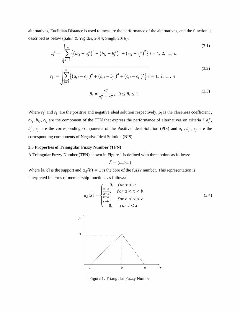
3.3 Properties of Triangular Fuzzy Number (TFN)

A Triangular Fuzzy Number (TFN) shown in Figure 1 is defined with three points as follows:

�̃� = (𝑎, 𝑏, 𝑐)

Where [a, c] is the support and 𝜇�̃�(𝑏) = 1 is the core of the fuzzy number. This representation is

interpreted in terms of membership functions as follows:

𝜇�̃�(𝑥) =

{

0, 𝑓𝑜𝑟 𝑥 < 𝑎 𝑥−𝑎

𝑏−𝑎, 𝑓𝑜𝑟 𝑎 < 𝑥 < 𝑏

𝑐−𝑥

𝑐−𝑏, 𝑓𝑜𝑟 𝑏 < 𝑥 < 𝑐

0, 𝑓𝑜𝑟 𝑐 < 𝑥

(3.4)

Figure 1. Triangular Fuzzy Number

The operation of the TFN could be summarized as follows (Mahapatra, Mahapatra, & Roy, 2016): let 𝐴 =

(𝑎1, 𝑏1, 𝑐1), 𝐵 = (𝑎2, 𝑏2, 𝑐2), r is a real number, then,

1) Addition: 𝐴 + 𝐵 = (𝑎1 + 𝑎2, 𝑏1 + 𝑏2, 𝑐1 + 𝑐2)

2) Subtraction: 𝐴 − 𝐵 = (𝑎1 − 𝑐2, 𝑏1 − 𝑏2, 𝑐1 − 𝑎2) (3.5)

3) Multiplication: 𝐴 × 𝐵 = (𝑎1 × 𝑎2, 𝑏1 × 𝑏2, 𝑐1 × 𝑐2)

𝐴 × 𝑟 = (𝑎1 × 𝑟, 𝑏1 × 𝑟, 𝑐1 × 𝑟)

The underlying reason for using TFN instead of other fuzzy techniques is primarily due to the probability-

possibility consistency principle that induces TFN from time series data. Moreover, TFN also provides the

basis for converting granular information that are extracted from graphically presented historical data.

3.4 Membership function and reliability modification

The definition of membership function was first introduced by L. A. Zadeh (1965), where the membership

functions were used to operate on the domain of all possible values. In fuzzy logic, membership degree

represents the truth value of a certain proposition.

Different from the concept of probability, truth value represents membership in vaguely defined sets. For

any set X, the membership degree of an element x of X in fuzzy set A is denoted as 𝜇𝐴(𝑥), which quantifies

the grade of membership of the element x to the fuzzy set A. To calculate the membership degree, the

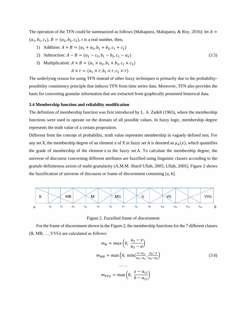
universe of discourse concerning different attributes are fuzzified using linguistic classes according to the

granule definiteness axiom of multi-granularity (A.M.M. Sharif Ullah, 2005; Ullah, 2005). Figure 2 shows

the fuzzification of universe of discourse or frame of discernment consisting [a, b].

Figure 2. Fuzzified frame of discernment

For the frame of discernment shown in the Figure 2, the membership functions for the 7 different classes

(B, MB, …,VVG) are calculated as follows:

𝑚𝐵 = 𝑚𝑎𝑥 (0, 𝑎3 − 𝑥

𝑎3 − 𝑎)

𝑚𝑀𝐵 = max (0, min(𝑥−𝑎1

𝑎3−𝑎1,𝑎5−𝑥

𝑎5−𝑎3) (3.6)

……

𝑚𝑉𝑉𝐺 = max (0, 𝑥 − 𝑎11𝑏 − 𝑎11

)

where 𝑎𝑖 = 𝑎 +𝑏−𝑎

2×7, 𝑖 = 1,2, … , (2 × 7 − 1), and 7 is the number of class in this frame of discernment.

The membership functions are assumed to be triangular and symmetric. The membership function for each

class depends on the frame of discernment of the attribute.

As the membership functions are assumed triangular and symmetric for the fuzzified frame of discernment,

the uncertainty and impreciseness of the functions need to be taken into consideration. Wen, Miaoyan, and

Chunhe (2017) proposed a reliability-based modification to deal with uncertainty of information and the

reliability of information sources. The reliability of the membership functions is measured by the static

reliability index and dynamic reliability index. Static reliability index is defined by the similarity among

classes, while dynamic reliability index is measured by the risk distance between the test samples and the

overlapping area among classes, respectively. The comprehensive reliability is computed by the product of

the two index, and the reliability-based membership function are fused using Dempster’s combination rule

(Dempster, 1967; Wen et al., 2017). The numerical examples provided by Jiang et al. (2018) verified the

effectiveness of the reliability modification approach in membership functions.

The static reliability index is measured by the overlapped area between two adjacent classes. In Figure 3,

the shaded area is the overlapped region between classes M and MG.

Figure 3. Illustration of static reliability index

The larger the overlapped area between classes M and MG, the more likely that an input data is wrongly

recognized in a linguistic class. The similarity between classes M and MG 𝑠𝑖𝑚𝑀,𝑀𝐺 in a certain attribute

and the corresponding static reliability index 𝑅𝑗𝑠 for 𝐶𝑗 can be described according to Wen et al. (2017):

𝑠𝑖𝑚𝑀,𝑀𝐺 =∫ min

𝑐≤𝑥≤𝑑(𝑚𝑀(𝑥),𝑚𝑀𝐺(𝑥))𝑑𝑥

𝑑

𝑐

∫𝑚𝑀(𝑥)+𝑚𝑀𝐺(𝑥)−∫ min𝑐≤𝑥≤𝑑

(𝑚𝑀(𝑥),𝑚𝑀𝐺(𝑥))𝑑𝑥𝑑

𝑐

(3.7)

𝑅𝑗𝑠 = ∑ (1 − 𝑠𝑖𝑚𝑖𝑙)𝑖<𝑙 (3.8)

where 𝑖 and 𝑙 are the adjacent classes in the same universe of discourse in one attribute.

The dynamic reliability index is measured with a set of test sample and calculated by the risk distance

between the peak of overlap area and the test value.

Figure 4. Illustration of dynamic reliability index

If 𝑃𝑀,𝑀𝐺 is the peak of the overlap area between classes M and MG in Figure 4, and 𝑇𝑗 is the test sample

generated for 𝐶𝑗 , the distance 𝑑 between 𝑇𝑗 and 𝑃𝑀,𝑀𝐺 represents the risk distance that related to the

uncertainty of the test sample. The risk distance and dynamic reliability index for 𝐶𝑗 can be formulated as:

𝑑𝑀,𝑀𝐺 =|T𝑗−𝑃𝑀,𝑀𝐺|

𝐷 (3.9)

𝑅𝑗𝑑 = 𝑒∑ 𝑑(𝑙−1)𝑙

𝑛2 (3.10)

where D is the range of the universe of discourse of C𝑗, which is (a − b) in Figure 3.

Then the comprehensive reliability index for 𝐶𝑗 can be defined as:

𝑅𝑗 = 𝑅𝑗𝑠 × 𝑅𝑗

𝑑 (3.11)

After the normalization we get,

𝑅𝑗∗ =

𝑅𝑗

max (𝑅𝑗) (3.12)

Then, the reliability-modified membership degree can be calculated as:

𝑚𝑗𝑙

𝑅𝑗∗

= 𝑅𝑗∗ ×𝑚𝑙 (3.13)

where l is a linguistic class in a universe of discourse.

4. Quantitative data analytics

4.1 Processing time-series data

A. M. M. Sharif Ullah and Shamsuzzaman (2013) proposed an approach that can represent the uncertainty

under a large set of continuous time-series input parameters (temporal data) by point cloud and transfer it

to a graphical fuzzy number based on probability-possibility transformation. The transformation process

is generalized as follows:

Assume, we have a temporal data presented in time-series data as shown in Figure 5.

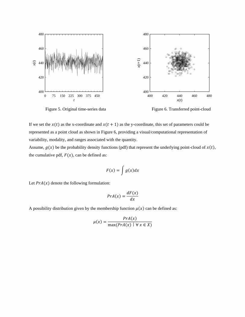
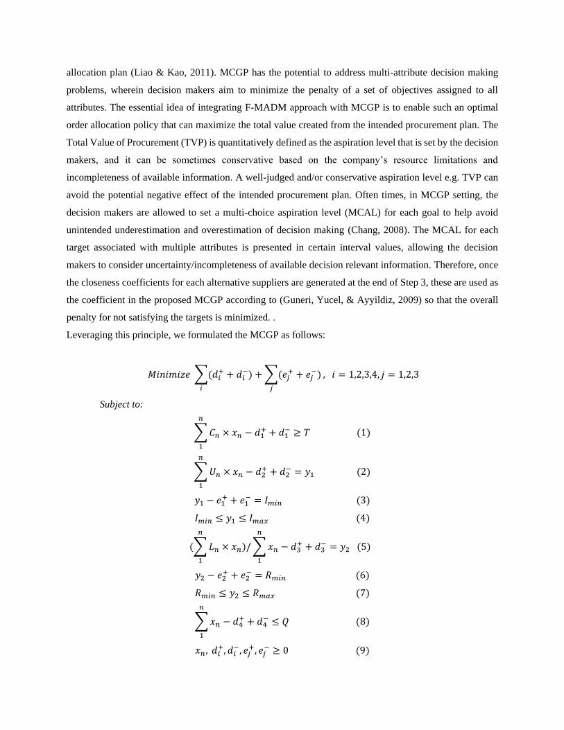
Figure 5. Original time-series data Figure 6. Transferred point-cloud

If we set the 𝑥(𝑡) as the x-coordinate and 𝑥(𝑡 + 1) as the y-coordinate, this set of parameters could be

represented as a point cloud as shown in Figure 6, providing a visual/computational representation of

variability, modality, and ranges associated with the quantity.

Assume, 𝑔(𝑥) be the probability density functions (pdf) that represent the underlying point-cloud of 𝑥(𝑡),

the cumulative pdf, 𝐹(𝑥), can be defined as:

𝐹(𝑥) = ∫𝑔(𝑥)𝑑𝑥

Let 𝑃𝑟𝐴(𝑥) denote the following formulation:

𝑃𝑟𝐴(𝑥) =𝑑𝐹(𝑥)

𝑑𝑥

A possibility distribution given by the membership function 𝜇(𝑥) can be defined as:

𝜇(𝑥) =𝑃𝑟𝐴(𝑥)

max (𝑃𝑟𝐴(𝑥)丨∀ 𝑥 ∈ 𝑋)

t

x(t)

0 75 150 225 300 375 450

400

420

440

460

480

x(t)

x(t+

1)

400 420 440 460 480

400

420

440

460

480

Figure 7. Graphical Triangular Fuzzy Number.

After the probability-possibility transformation, the point cloud is transferred to a triangular possibility

distribution or TFN in a graphical format as shown in Figure 7. In what follows, the triangular fuzzy set

can be expressed as:

𝐴 = (425, 442, 452)

x

mul(

x)

420 425 430 435 440 445 450 455

-0.2

0

0.2

0.4

0.6

0.8

1

1.2

4.2 Processing graphical information

Figure 8. Graphical information extraction process.

In the logistics 4.0 system, the data are not always generated in the format of continuous time-series.

Sometimes they are generated discretely and stored in the data base for future access. These historically

stored data can be expressed in pieces of graphs (Domingo Galindo, 2016) because when visualized, these

pieces of graphs can potentially present a large amount of information in an easy-to-understand way. Then,

the necessary DRI in terms of pieces of crisp granular information can be extracted from these graphically

(a) Data visualization for all

suppliers

(b) Extracting graph for a

single supplier

(c) Crisp granular information

concerning cost (d) Crisp granular information

concerning production capacity

presented data according to (Ullah & Noor-E-Alam, 2018). Figure 8(a) shows the visualization of data

collected for five suppliers concerning cost per unit of product and production capacity. Then, graphical

data associated with a single supplier can be extracted from the combined graph and is presented in Figure

8(b). Once data for individual supplier is presented graphically, then the associated DRI concerning cost

per unit of product and production capacity can be extracted in the form of crisp granular information or

ranges as visualized in Figure 8(c) and Figure 8(d), respectively.

5.0 Proposed supplier evaluation and order allocation model

In this Supplier Evaluation and Order Allocation Model, both the quantitative and qualitative information

are characterized by Triangular Fuzzy Number (TFN) to evaluate the performance of the alternatives in a

unified platform, simultaneously. For the quantitative attributes, time-series and non-time series data are

transferred to fuzzy set through point cloud and graphic extraction approaches, respectively, while

qualitative assessments, including performance and weight appraisal, are transferred directly based on the

standard fuzzification process of the frame of discernment. With the fuzzy set for all attributes and weights,

the weighted decision matrix is constructed. Then the algorithm of TOPSIS is performed to evaluate the

performance of the alternatives and generate the list of preference based on the obtained ranking score.

Finally, the ranking score are regarded as the coefficient in the MCGP to calculate the order allocation plan

that best fulfill the requirements of the decision makers. To provide a comprehensive and understandable

illustration for the proposed supplier evaluation and order allocation model, we present a complete

computation process with detailed description below:

Step 1: Processing Quantitative data

In this step, we process and transfer the large number of quantitative data entailing time-series and non-

time series data, which are available in pieces of graphics. Following two sub-steps constitute this step.

Step 1(a): Transferring time-series based quantitative data to TFN

At first, the time-series data, for supplier 𝑆𝑖 on attribute 𝐶𝑗 are expressed by a point cloud in the form of

𝑃(𝑥(𝑡), 𝑥(𝑡 + 1)) according to the principle explained in section 4.1. After the point cloud transformation,

the data are transferred to a possibility distribution of triangular form as shown in Figure 7, which can be

represented by a TFN in the form of 𝐴𝑖𝑗 (𝑎𝑖𝑗 , 𝑏𝑖𝑗 , 𝑐𝑖𝑗).

Step 1(b): Transferring non-time series based graphical data to TFN

After the information extracted from the graphical information in the form of crisp granular information,

the randomly obtained 𝑟 number of crisp granular information or ranges for supplier 𝑆𝑖 on attribute 𝐶𝑗,

𝑅𝑖𝑗𝑟(𝑝𝑖𝑗𝑟 , 𝑞𝑖𝑗𝑟), are presented in Table 2.

Table 2. Example of extracted ranges

Ranges 𝐶𝑗

𝑅𝑖𝑗1 (𝑝𝑖𝑗1, 𝑞𝑖𝑗1) 𝑅𝑖𝑗2 (𝑝𝑖𝑗2, 𝑞𝑖𝑗2) … …

𝑅𝑖𝑗𝑟 (𝑝𝑖𝑗𝑟 , 𝑞𝑖𝑗𝑟)

After collecting all the crisp granular information for every alternative supplier, we fuzzify the frame of

discernment associated with every non-time series attribute 𝐶𝑗 based on the fuzzification approach

proposed in (Ullah & Noor-E-Alam, 2018). In the fuzzification process, the span of the frame of

discernment is generated by the minimum and maximum of all the extracted crisp granular information

for a certain attribute regarding all the alternative suppliers, while the number of linguistic terms is

determined according to the granule definiteness axiom (A.M.M. Sharif Ullah, 2005; Ullah, 2005). For

Example, if 𝑝𝑚𝑖𝑛 = min𝑟𝑝𝑖𝑗𝑟, 𝑞𝑚𝑎𝑥 = max

𝑟𝑞𝑖𝑗𝑟, the frame of discernment of 𝐶𝑗 presented as 𝑈 =

[𝑝𝑚𝑖𝑛, 𝑞𝑚𝑎𝑥] can be fuzzified as shown in Figure 9.

After the fuzzification process, the linguistic classes 𝑙 and associated TFN table are constructed as in

Table 3:

Table 3.

Linguistic terms and associated TFN

Where B and MB represent linguistic terms expressed as Bad, Moderately Bad, and 𝑙𝑚is 𝑚𝑡ℎ linguistic

term that can assume the form such as Bad (B), Moderately Bad (MB), Moderately Good (MG), Good

(G) etc.

Linguistic Terms 𝑇𝐹𝑁 (𝑎, 𝑏, 𝑐)

𝐵 𝑎𝐵 𝑏𝐵 𝑐𝐵

𝑀𝐵 𝑎𝑀𝐵 𝑏𝑀𝐵 𝑐𝑀𝐵

… … … …

𝑙𝑚 𝑎𝑙𝑚 𝑏𝑙𝑚 𝑐𝑙𝑚

Figure 9. Fuzzified frame of discernment.

With the fuzzified frame of discernment, the membership degree for every range value 𝑅𝑖𝑗𝑟(𝑝𝑖𝑗𝑟 , 𝑞𝑖𝑗𝑟) on

each linguistic class is computed based on (3.6).

𝑚𝑖𝑗 =∫ 𝑚𝐹(𝑥)𝑑𝑥

𝑥∈𝑅

‖�́�‖ (5.1)

where R refers to the span of the criteria and ‖�́�‖ refers to the largest segment of R that belongs to the

support 𝑚𝐹 . This way, the membership degree of 𝑅𝑖𝑗𝑟(𝑝𝑖𝑗𝑟 , 𝑞𝑖𝑗𝑟) on attribute C𝑗 at linguistic class l is

calculated as 𝑀𝑖𝑗𝑟𝑙 .

Because all the membership functions are assumed to be symmetric and triangular, we perform reliability

modification for the calculated membership degrees. According to equations (3.7-3.12), the comprehensive

reliability indexes for C𝑗 could be generated as Rc𝑗. Multiplied with the obtained Rc𝑗 based on (3.13), the

original membership degree 𝑀𝑖𝑗𝑟𝑙 can be modified as 𝑀𝑖𝑗𝑟𝑙′ . As there are 𝑟 computed modified membership

degrees for each linguistic class, we aggregate them as follows:

𝑀𝑖𝑗𝑟𝑙∗ = ∑ 𝑀𝑖𝑗𝑙

′𝑟 (5.2)

Then, the reliability modified membership degrees are normalized to induce TFN for the integrated TOPSIS

decision matrix as mentioned below:

𝑁𝑖𝑗𝑙 =𝑀𝑖𝑗𝑙∗

∑𝑀𝑖𝑗𝑙∗ , ∑𝑁𝑖𝑗𝑙 = 1 (5.3)

To generate the TFN for the attribute involving non-time series graphical information, we utilized the TFN

for every linguistic class in Table 3 and the membership degrees calculated above. In this integration

process, without loss of information generality, the membership degree is regarded as the weight of each

linguistic class for every alternative concerning each attribute. Then the membership degree is converted to

TFN that will be used in the TFN based TOPSIS decision matrix. The integrated TFN is presented

as 𝐴𝑖𝑗 (𝑎𝑖𝑗 , 𝑏𝑖𝑗 , 𝑐𝑖𝑗):

𝑎𝑖𝑗 = ∑ 𝑎𝑙𝑁𝑖𝑗𝑙𝑙

𝑏𝑖𝑗 = ∑ 𝑏𝑙𝑁𝑖𝑗𝑙𝑙 (5.4)

𝑐𝑖𝑗 = ∑ 𝑐𝑙𝑁𝑖𝑗𝑙𝑙

Where 𝑙 is the linguistic class in Table 3.

Step 2: Processing qualitative data

Step 2 process and transfer qualitative data associated with supplier performance and importance weight of

underlying attributes evaluation provided by multiple decision makers (DM). Following two sub-steps

entails step 2.

Step 2(a): Processing and transferring qualitative data entailing suppliers’ performance evaluation to

aggregated TFN

The qualitative assessments given by the decision makers for each supplier against each attribute are

directly transferred to respective TFNs. For example, a set of qualitative assessments for 𝑖𝑡ℎ suppliers on

attribute C𝑗 given by 𝑘𝑡ℎ DM can be represented as in Table 4. The qualitative assessment given by 𝐿𝑖𝑗𝑘

can assume any of the form given by Bad (B), Moderately Bad (MB), Moderate (M), Moderately Good

(MG), Good (G), Very Good (VG), Very Very Good (VVG), and Extremely Good (EG).

Table 4

Example of original linguistic data

C𝑗

𝑆𝑢𝑝𝑝𝑙𝑖𝑒𝑟/𝐷𝑀𝑠 𝐷𝑀1 𝐷𝑀2 … 𝐷𝑀𝑘

𝑆1 𝐿1𝑗1 𝐿1𝑗2 … 𝐿1𝑗𝑘

𝑆2 𝐿2𝑗1 𝐿2𝑗2 … 𝐿2𝑗𝑘

… … … … …

𝑆𝑖 𝐿𝑖𝑗1 𝐿𝑖𝑗2 … 𝐿𝑖𝑗𝑘

These qualitative appraisals are then converted to respective TFNs using standard TFN (Table 14 in

Appendix A) associated with different linguistic classes, similar to (C.-T. Chen et al., 2006). The converted

TFN can be presented as in Table 5. In doing so, the uncertainty associated with vague qualitative

assessment is also quantified with the help TFN.

Table 5

Example of TFN decision matrix

C𝑗

𝑆𝑢𝑝𝑝𝑙𝑖𝑒𝑟/𝐷𝑀𝑠 𝐷𝑀1 𝐷𝑀2 … 𝐷𝑀𝑘

𝑆1 (𝑎1𝑗1, 𝑏1𝑗1, 𝑐1𝑗1) (𝑎1𝑗2, 𝑏1𝑗2, 𝑐1𝑗2) … (𝑎1𝑗𝑘 , 𝑏1𝑗𝑘 , 𝑐1𝑗𝑘)

𝑆2 (𝑎2𝑗1, 𝑏2𝑗1, 𝑐2𝑗1) (𝑎2𝑗2, 𝑏2𝑗2, 𝑐2𝑗2) … (𝑎2𝑗𝑘 , 𝑏2𝑗𝑘 , 𝑐2𝑗𝑘)

… … … … …

𝑆𝑖 (𝑎𝑖𝑗1, 𝑏𝑖𝑗1, 𝑐𝑖𝑗1) (𝑎𝑖𝑗2, 𝑏𝑖𝑗2, 𝑐𝑖𝑗2) … (𝑎𝑖𝑗𝑘 , 𝑏𝑖𝑗𝑘 , 𝑐𝑖𝑗𝑘)

Finally, the TFN-based TOPSIS decision matrix is constructed by incorporating and aggregating the

conflicting qualitative assessments provided by all the DMs involved in the decision-making process. This

is similar to what is proposed by C.-T. Chen et al. (2006) as follows:

𝐴𝑖𝑗 (𝑎𝑖𝑗 , 𝑏𝑖𝑗 , 𝑐𝑖𝑗) = (min𝑘𝑎𝑖𝑗𝑘 ,

∑ 𝑏𝑖𝑗𝑘𝑘

𝑘, max

𝑘𝑐𝑖𝑗𝑘) (5.5)

Step 2(b): Transferring qualitative data on attributes’ weight to TFN

The weights of all the attributes are determined and expressed by the DMs in the form of qualitative

assessment as well. Such qualitative assessment can be expressed in the form of linguistics terms e.g., Very

Unimportant (VUI), Unimportant (UI), Moderately Important (MI), Important (I), Very Important (VI), and

Extremely Important (EI). Some of these linguistic terms and associated TFNs are listed in Table 6. Since

the weight lies in between 0 to 1, the frame of discernment is represented as 𝑈 = [0,1]. Using these TFNs

we fuzzified the frame of discernment of the attribute weights as shown in Figure 10:

Table 6.

Linguistic terms and corresponding fuzzified TFN

Then the weight of each attribute is at first directly converted to a TFN, 𝑤𝑗(𝑎𝑗 , 𝑏𝑗 , 𝑐𝑗) using the TFN

associated with respective linguistic term. Once all the qualitative weights provided by multiple DMs are

converted to respective TFNs, the aggregated weight and corresponding TFNs are generated according to

equation 5.5 as mentioned in step 2(a).

Step 3: Performing TOPSIS to rank alternative suppliers

Because in the weighted decision matrix, the TFNs concerning each supplier against each attribute have

different support defined as [𝑎𝑖𝑗, 𝑐𝑖𝑗] ,we first normalized each TFN 𝐴𝑖𝑗 (𝑎𝑖𝑗 , 𝑏𝑖𝑗 , 𝑐𝑖𝑗) on all attributes

before performing TOPSIS based on the principle used in (C.-T. Chen et al., 2006):

Weight of Criteria

Linguistic Terms TFN (a, b, c)

VUI (0,0.1,0.2)

UI (0.1,0.2,0.3)

… …

EI (0.8,0.9,1)

Figure 10. Fuzzification of criteria weight.

Weight

mu

l(.)

0 0.1 0.2 0.3 0.4 0.5 0.6 0.7 0.8 0.9 1

-0.2

0

0.2

0.4

0.6

0.8

1

1.2

VUI UI MUI M MI I VI VVI EI

𝐴𝑖𝑗′ (𝑎𝑖𝑗

′ , 𝑏𝑖𝑗′ , 𝑐𝑖𝑗

′ ) = (𝑎𝑖𝑗

max𝑖𝑐𝑖𝑗,

𝑏𝑖𝑗

max𝑖𝑐𝑖𝑗,

𝑐𝑖𝑗

max𝑖𝑐𝑖𝑗) , ∀ 𝑗 ∈ 𝐺1 (5.6)

𝐴𝑖𝑗′ (𝑎𝑖𝑗

′ , 𝑏𝑖𝑗′ , 𝑐𝑖𝑗

′ ) = (min𝑖𝑎𝑖𝑗

𝑐𝑖𝑗 ,min𝑖𝑎𝑖𝑗

𝑏𝑖𝑗,min𝑖𝑎𝑖𝑗

𝑎𝑖𝑗) , ∀ 𝑗 ∈ 𝐺2 (5.7)

where 𝐺1 is the set of beneficial attributes which will be maximized and 𝐺2 is the set of non- beneficial

attributes which will be minimized.

As now we have the normalized TFN 𝐴𝑖𝑗′ (𝑎𝑖𝑗

′ , 𝑏𝑖𝑗′ , 𝑐𝑖𝑗

′ ) for all suppliers 𝑆𝑖 on every attribute 𝐶𝑗, and the

attribute weight 𝑤𝑗(𝑎𝑗 , 𝑏𝑗 , 𝑐𝑗), the normalized and weighted TFN based TOPSIS decision matrix {𝐴𝑖𝑗∗ } is

constructed based on (3.5):

𝐴𝑖𝑗∗ (𝑎𝑖𝑗

∗ , 𝑏𝑖𝑗∗ , 𝑐𝑖𝑗

∗ ) = 𝐴𝑖𝑗′ × 𝑤𝑗 (5.9)

The Positive Ideal Solution (PIS) and Negative Ideal Solution (NIS) are determined as (C.-T. Chen et al.,

2006):

𝐴𝑝𝑗(𝑎𝑝𝑗 , 𝑏𝑝𝑗 , 𝑐𝑝𝑗) = max𝑖𝑐𝑖𝑗∗

𝐴𝑛𝑗(𝑎𝑛𝑗 , 𝑏𝑛𝑗 , 𝑐𝑛𝑗) = min𝑖𝑎𝑖𝑗∗ (5.10)

And, finally the closeness coefficient (�̃�𝑖) for 𝑆𝑖 is generated as:

𝑑𝑖+ = √

∑ (𝑎𝑖𝑗∗ −𝑎𝑝𝑗)

2+∑ (𝑏𝑖𝑗∗ −𝑏𝑝𝑗)

2𝑗 +∑ (𝑐𝑖𝑗

∗ −𝑐𝑝𝑗)2

𝑗𝑗

3

𝑑𝑖− = √

∑ (𝑎𝑖𝑗∗ −𝑎𝑛𝑗)

2+∑ (𝑏𝑖𝑗

∗ −𝑏𝑛𝑗)2

𝑗 +∑ (𝑐𝑖𝑗∗ −𝑐𝑛𝑗)

2

𝑗𝑗

3 (5.11)

�̃�𝑖 =𝑑𝑖−

(𝑑𝑖−+𝑑𝑖

+)

The higher the �̃�𝑖, the higher will be the ranking for a particular supplier. Ranking is given as an ascending

order starting from 1 for a supplier with highest �̃�𝑖, and follows chronological order for rest of the suppliers.

Step 4: Performing MCGP to determine optimal order allocation policy

It is perhaps not surprising that a single supplier may not always have the ability to supply the entire ordered

quantity. In addition, strategic decision makers may opt for diversifying the sourcing channels while

ensuring stability and competitiveness among alternative suppliers under the threat of disruption risks.

These altogether make it feasible that decision makers often times have to depend on multiple suppliers,

requiring an optimal order allocation strategy that takes into account the supplier preferential ranking 𝑅𝑖

generated via F-MADM approach as input. Multi-choice Goal Programming (MCGP)—a viable approach

in this regard—can successfully be integrated with F-MADM based DSS to devise an optimal order

allocation plan (Liao & Kao, 2011). MCGP has the potential to address multi-attribute decision making

problems, wherein decision makers aim to minimize the penalty of a set of objectives assigned to all

attributes. The essential idea of integrating F-MADM approach with MCGP is to enable such an optimal

order allocation policy that can maximize the total value created from the intended procurement plan. The

Total Value of Procurement (TVP) is quantitatively defined as the aspiration level that is set by the decision

makers, and it can be sometimes conservative based on the company’s resource limitations and

incompleteness of available information. A well-judged and/or conservative aspiration level e.g. TVP can

avoid the potential negative effect of the intended procurement plan. Often times, in MCGP setting, the

decision makers are allowed to set a multi-choice aspiration level (MCAL) for each goal to help avoid

unintended underestimation and overestimation of decision making (Chang, 2008). The MCAL for each

target associated with multiple attributes is presented in certain interval values, allowing the decision

makers to consider uncertainty/incompleteness of available decision relevant information. Therefore, once

the closeness coefficients for each alternative suppliers are generated at the end of Step 3, these are used as

the coefficient in the proposed MCGP according to (Guneri, Yucel, & Ayyildiz, 2009) so that the overall

penalty for not satisfying the targets is minimized. .

Leveraging this principle, we formulated the MCGP as follows:

𝑀𝑖𝑛𝑖𝑚𝑖𝑧𝑒 ∑(𝑑𝑖+ + 𝑑𝑖

−)

𝑖

+∑(𝑒𝑗+ + 𝑒𝑗

−)

𝑗

, 𝑖 = 1,2,3,4, 𝑗 = 1,2,3

Subject to:

∑𝐶𝑛 × 𝑥𝑛 − 𝑑1+ + 𝑑1

− ≥ 𝑇

𝑛

1

(1)

∑𝑈𝑛 × 𝑥𝑛 − 𝑑2+ + 𝑑2

− = 𝑦1

𝑛

1

(2)

𝑦1 − 𝑒1+ + 𝑒1

− = 𝐼𝑚𝑖𝑛 (3)

𝐼𝑚𝑖𝑛 ≤ 𝑦1 ≤ 𝐼𝑚𝑎𝑥 (4)

(∑𝐿𝑛 × 𝑥𝑛)/∑𝑥𝑛

𝑛

1

− 𝑑3+ + 𝑑3

− = 𝑦2 (5)

𝑛

1

𝑦2 − 𝑒2+ + 𝑒2

− = 𝑅𝑚𝑖𝑛 (6)

𝑅𝑚𝑖𝑛 ≤ 𝑦2 ≤ 𝑅𝑚𝑎𝑥 (7)

∑𝑥𝑛 − 𝑑4+ + 𝑑4

− ≤ 𝑄

𝑛

1

(8)

𝑥𝑛 , 𝑑𝑖+, 𝑑𝑖

−, 𝑒𝑗+, 𝑒𝑗

− ≥ 0 (9)

Where:

𝑑𝑖+, 𝑑𝑖

−, 𝑒𝑚+ , 𝑒𝑚

− stand for the penalties in violation of respective constraints

𝑥𝑛 is the optimal ordered quantity assigned to nth Supplier

𝐶𝑛 is the closeness coefficients (�̃�𝑖) of the available suppliers

𝑇 is the total value created from procurement (TVP)

𝑈𝑛 is the unit cost of quantity when purchased from nth supplier

𝑦1 is the total available budget for the procurment

𝐼𝑚𝑖𝑛 , 𝐼𝑚𝑎𝑥 𝑎𝑟𝑒 𝑡ℎ𝑒 𝑙𝑜𝑤𝑒𝑟 𝑙𝑖𝑚𝑖𝑡 𝑎𝑛𝑑 𝑢𝑝𝑝𝑒𝑟 𝑙𝑖𝑚𝑖𝑡 𝑜𝑛 𝑡ℎ𝑒 𝑏𝑢𝑑𝑔𝑒𝑡, 𝑟𝑒𝑠𝑝𝑒𝑐𝑡𝑖𝑣𝑒𝑙𝑦

𝐿𝑛 is lead time of the nth supplier

𝑦2 is the total allowable lead time for a particualr order

𝑅𝑚𝑖𝑛, 𝑅𝑚𝑎𝑥 𝑎𝑟𝑒 𝑡ℎ𝑒 lower limit and upper limit on lead time, respectively

𝑄 𝑖s the procurement level set by the decision makers

𝑛 is the number of alternative suppliers

The objective function aims to minimize the total non-achievement penalties of multiple targets assigned

in different constraints. Constraint (1) ensures that the orders should be allocated among multiple suppliers

considering their preferential ranking in such a way so that a minimum TVP is achieved. In other words,

constraint (1) sets an upper bound on TVP. Meanwhile, constraint (2) refers to the goal of procurement

budget, signifying that total procurement cost will not exceed the budget after including the positive and

negative deviation of the intended goal. Constraints (3) and (4) explains the aspiration levels of the goal

associated with procurement budget. In a similarly way, constraint (5), (6) and (7) illustrate the lead time

preference along with the aspiration levels associated with corresponding lead times. Finally, constraint (8)

with consideration of deviations from the procurement level goal, restrict that the total order allocated to

multiple suppliers must equal the procurement level set by the decision makers.

Such an MCGP model is anticipated to handle multiple objectives if a decision maker seeks the optimal

solution from a set of feasible solutions considering the aspiration levels of the objectives; thus, enabling

the management to optimally balance their requirements among alternative suppliers when the multiple

requirements cannot be satisfied by a single supplier.

The proposed decision-making framework is presented as a flow chart in Figure 11:

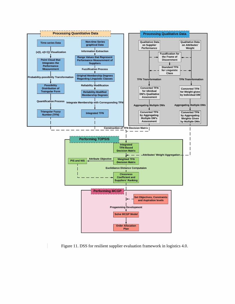
Figure 11. DSS for resilient supplier evaluation framework in logistics 4.0.

6. Case illustration

To demonstrate the effectiveness and usefulness of the proposed supplier evaluation and order allocation

DSS, we present a hypothetical case study that is generalizable to companies operating under logistics 4.0.

Such logistics 4.0 companies concern different aspects of end-to-end logistics and supply chain

management, which transforms the way those companies manage their logistics operations. This

transformation is powered by the digitalization of supply chain system—characterized by the speed,

flexibility, real-time connectedness among different entities of logistics 4.0—arguably, supply chain 4.0.

Crucially, effective sourcing of raw materials plays a significant role in achieving that desired level of

efficiency, responsiveness and resilience in the context of connected, decentralized and digitalized supply

chain. Often times, a set of alternative suppliers may serve the purpose of providing a particular raw

material. Strategic decision makers responsible for taking such high-impact sourcing decisions must choose

a supplier among available alternatives who can best serve the requirement of resilience, sustainability and

efficiency. Therefore, the supplier evaluation and selection process in this context of logistics 4.0 is

characterized as a decision-making problem comprising multiple conflicting attributes. The problem

becomes even more complex when a single supplier is not able to provide entire ordered quantity, and

allocation of order is needed among multiple suppliers.

6.1 Evaluation attributes

As alluded previously, we select and define several attributes based on which the alternative suppliers are

evaluated from logistics 4.0 and resilience perspectives. Attributes are divided into two main groups: (1)

quantitative and (2) qualitative as presented in Table 7. For attributes in the quantitative subset, large

number of data is available in the form of continuous time series. Data collected historically are

characterized as non-time series data. These historically collected data are often stored graphically in

logistics 4.0 environment due to the digitalization, cloud storage facilities and Internet of Things (IOT).

Moreover, when visualized graphically, these data entail a great deal of actionable information that has

been proven to be valuable while evaluating several sourcing options. As such, quantitative criteria are then

sub-divided into two groups based on the type of data available as decision relevant information. We

characterized that for inventory and delivery schedules, data are collected continuously and presented in

time series as real-time visibility and end-to-end data sharing are considered as crucial aspects of logistics

4.0. On the other hand, data associated with supplier’s production capacity and cost are collected over the

time and can be presented graphically. In case of other fifteen attributes listed in Table 7, qualitative

assessments are given by multiple decision makers for each alternative supplier. All those attributes are so

chosen that has been used to measure the resilience performance of the suppliers in the context of logistics

4.0.

To further specify the effect of these attributes in enhancing resilience i.e., reducing vulnerability against

anticipated disruptions and improving recoverability after being affected by disruption, we categorize and

associate them to pre-disaster and post-disaster resilience activities. Attributes 𝐶2, 𝐶5, 𝐶6, 𝐶7, 𝐶8, 𝐶9, 𝐶11,

𝐶12, 𝐶13, and 𝐶15 are used to evaluate alternative suppliers based on their ability to reduce the vulnerability

against potential disruptions, and thus refer to the pre-disaster resilience activities of the suppliers. On the

other hand, attributes 𝐶1, 𝐶3, 𝐶10, 𝐶14, 𝐶16, 𝐶17, 𝐶18 and 𝐶19 are used to evaluate suppliers depending on

their ability to recover quickly and effectively after being affected by disruption, and thus represent

supplier’s post disaster resilience strategies. Cost (attribute 𝐶4) is considered as expense that supplier has

to incur to provide the goods, and also to ensure the desired level of resilience through coordinated pre-

disaster and post-disaster strategies.

Table 7.

List of attributes considered in decision making process

Types of

decision relevant

information

𝐶𝑗 Attributes Object

ive Description

Quantitati

ve

attributes

Time-series

data

𝐶1

Pre-positioned

inventory

level

Max The quantity of inventory in stock and

available for supply.

𝐶2 Lead time

variability Min

Time that supplier take to deliver the order to

the company.

Non-time-series

data presented

graphically

𝐶3 Production

capacity Max

Quantity of the products that a supplier is

capable to produce per day.

𝐶4 Cost Min

Cost that is incurred by the company while

purchasing the required quantity from a

particular supplier. The cost here included per

unit production and transportation cost.

Qualitative

attributes

Qualitative

assessment

presented in

linguistic terms

𝐶5 Digitalization Max

Enabled by Web technologies, work flow tools,

portals for customers, suppliers and employees,

and information technology innovations

targeted at supply chains and customer

relationships (Rai et al., 2006).

𝐶6 Traceability Max The ability to trace the origin of materials and

parts, processing history and distribution or

location of the product while being delivered

(Aung & Chang, 2014).

𝐶7 Supply chain

density Min

The quantity and geographical spacing of

nodes within a supply chain.

𝐶8 Supply chain

complexity Max

The number of nodes in a supply chain and the

interconnections between those nodes.

𝐶9 Re-

engineering Max

The corrective procedure for the incorporation

of any engineering design change within the

product. Suppliers need to possess re-

engineering capability to respond to customer’s

change of taste or requirements.

𝐶10

Supplier’s

resource

flexibility

Max

The different logistics strategies which can be

adopted either to release a product to a market

or to procure a component from a supplier.

𝐶11 Automation

disruption Min

Ability to withstand the disruption caused in

the automated manufacturing system.

𝐶12 Information

management Max

The ability to acquire, store, retrieve, process

and share fast flowing information regarding

demand and lead time volatility, change in

price, real time location sharing while

delivering the raw materials.

𝐶13

Cyber security

risk

management

Max

Ability to prevent or mitigate damage from IT

security breaches in supply chains, where

breaches can disrupt production, cause loss of

essential data, and compromise confidential

information.

𝐶14 Supplier

reliability Max

The availability during disruptions of

alternative transportation channels with

different characteristics based on their costs

and delivery dates.

𝐶15 Supply chain

visibility Max

The ability of the supplier to have a vivid view

of upstream and downstream inventories,

demand and supply conditions, and production

and purchasing schedules.

𝐶16 Level of

collaboration Max

Supplier collaboration reduces forecasting and

inventory management risks, thereby

enhancing resilience of supply chains. Also, it

helps mitigate supply side uncertainty after

disruption hits.

𝐶17 Restorative

capacity Max

The ability of suppliers to repair and quickly

restore to its normal operating conditions after

a disruptive event.

𝐶18

Rerouting

Max

Capability of changing the usual mode of

transport while anticipating or being affected

by the disruptions. Companies can combine

multiple modes of intermodal transportation

which are fast to ensure uninterrupted supply

of goods and operations of supply chain.

𝐶19 Agility Max

The speed with which a firm’s internal supply

chain functions can adapt to marketplace

changes resulting from disruption and thus can

better respond to unforeseen events

6.2 Results and sensitivity analysis

To test the practicability of our proposed model, we randomly generated a set of data in Appendix A. The

numerical example includes five alternative suppliers that are evaluated with regards to four quantitative

attributes and fifteen qualitative attributes presented in Table 7. For each supplier, 500 records are collected

as continuous time series in case of pre-positioned inventory level (attribute 𝐶1) and lead time variability

(attribute 𝐶2) (presented in Figure 15 & Figure 16 in Appendix A). As mentioned in sub-step 1(a) in section

5, these time-series data are transferred to possibility distribution of triangular form (Figure 18 & Figure 19

in Appendix B), which afterwards were used to induce TFNs (Table 15 in Appendix B). In case of

production capacity and cost, 300 records are used from historically collected data, which are presented in

several pieces of graphs, making it easier to process this large quantity of data into actionable decision

relevant information (Figure 17 in Appendix A). According to the sub-step 1(b) mentioned in section 5, the

crisp granular information extracted from these graphs concerning each supplier are presented in Table 16

(Appendix B). Then the integrated TFNs associated with each of these two attributes for all five alternative

suppliers are computed following the procedure described in sub-step 1(b) in section 5 and are presented in

Table 17 (Appendix B). Performance evaluation data concerning each supplier against each qualitative

attribute are collected from five decision makers who are assumed to have equal importance in decision

making process. As previously mentioned in section 5, these qualitative assessments are provided in the

form of linguistic appraisals, which are presented in Table 13 for attribute 𝐶5 to 𝐶19 (Appendix A). These

qualitative assessments are transferred to corresponding TFNs according to the process detailed in sub-step

2(a) in section 5. Similarly, the qualitative weights of all the attributes provided by multiple DMs in

linguistic terms are also listed in Table 13 (Appendix A), which later are converted to respective TFNs

according to the principle described in sub-step 2(b) in section 5 and presented in Table 18 (Appendix B).

After converting all the quantitative and qualitative DRI into respective TFNs, the weighted TFN-based

TOPSIS decision matrix is constructed, which was used to determine the PIS and NIS according to step 3

in section 5. The PIS and NIS associated with all the attributes are listed in Table 19 (Appendix B). Finally,

the closeness coefficients (�̃�𝑖) are calculated for each alternative supplier.

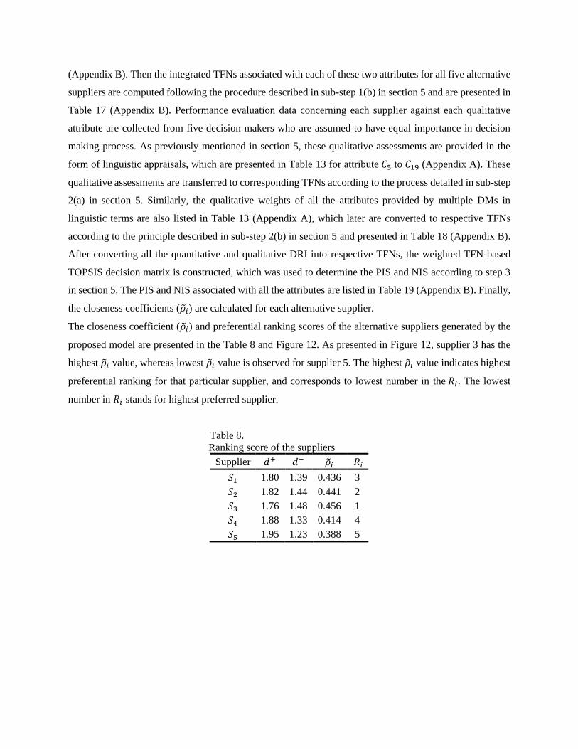
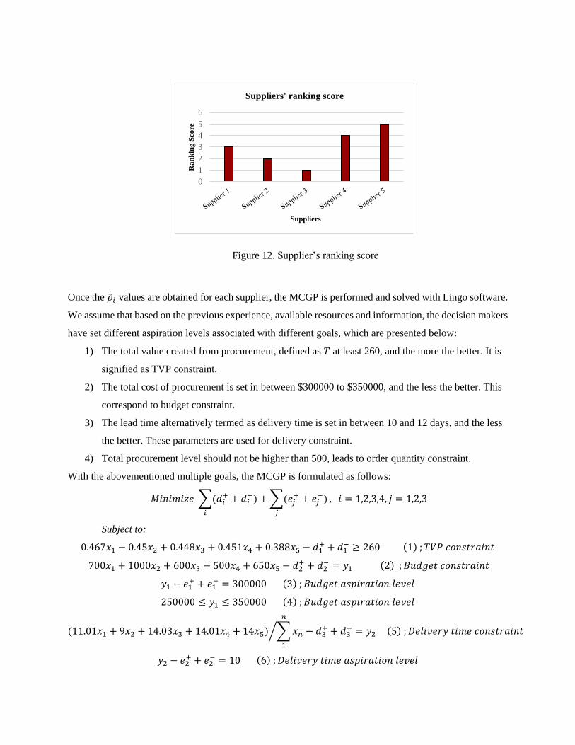
The closeness coefficient (�̃�𝑖) and preferential ranking scores of the alternative suppliers generated by the

proposed model are presented in the Table 8 and Figure 12. As presented in Figure 12, supplier 3 has the

highest �̃�𝑖 value, whereas lowest �̃�𝑖 value is observed for supplier 5. The highest �̃�𝑖 value indicates highest

preferential ranking for that particular supplier, and corresponds to lowest number in the 𝑅𝑖. The lowest

number in 𝑅𝑖 stands for highest preferred supplier.

Table 8.

Ranking score of the suppliers

Supplier 𝑑+ 𝑑− �̃�𝑖 𝑅𝑖

𝑆1 1.80 1.39 0.436 3

𝑆2 1.82 1.44 0.441 2

𝑆3 1.76 1.48 0.456 1

𝑆4 1.88 1.33 0.414 4

𝑆5 1.95 1.23 0.388 5

Once the �̃�𝑖 values are obtained for each supplier, the MCGP is performed and solved with Lingo software.

We assume that based on the previous experience, available resources and information, the decision makers

have set different aspiration levels associated with different goals, which are presented below:

1) The total value created from procurement, defined as 𝑇 at least 260, and the more the better. It is

signified as TVP constraint.

2) The total cost of procurement is set in between $300000 to $350000, and the less the better. This

correspond to budget constraint.

3) The lead time alternatively termed as delivery time is set in between 10 and 12 days, and the less

the better. These parameters are used for delivery constraint.

4) Total procurement level should not be higher than 500, leads to order quantity constraint.

With the abovementioned multiple goals, the MCGP is formulated as follows:

𝑀𝑖𝑛𝑖𝑚𝑖𝑧𝑒 ∑(𝑑𝑖+ + 𝑑𝑖

−)

𝑖

+∑(𝑒𝑗+ + 𝑒𝑗

−)

𝑗

, 𝑖 = 1,2,3,4, 𝑗 = 1,2,3

Subject to:

0.467𝑥1 + 0.45𝑥2 + 0.448𝑥3 + 0.451𝑥4 + 0.388𝑥5 − 𝑑1+ + 𝑑1

− ≥ 260 (1) ; 𝑇𝑉𝑃 𝑐𝑜𝑛𝑠𝑡𝑟𝑎𝑖𝑛𝑡

700𝑥1 + 1000𝑥2 + 600𝑥3 + 500𝑥4 + 650𝑥5 − 𝑑2+ + 𝑑2

− = 𝑦1 (2) ; 𝐵𝑢𝑑𝑔𝑒𝑡 𝑐𝑜𝑛𝑠𝑡𝑟𝑎𝑖𝑛𝑡

𝑦1 − 𝑒1+ + 𝑒1

− = 300000 (3) ; 𝐵𝑢𝑑𝑔𝑒𝑡 𝑎𝑠𝑝𝑖𝑟𝑎𝑡𝑖𝑜𝑛 𝑙𝑒𝑣𝑒𝑙

250000 ≤ 𝑦1 ≤ 350000 (4) ; 𝐵𝑢𝑑𝑔𝑒𝑡 𝑎𝑠𝑝𝑖𝑟𝑎𝑡𝑖𝑜𝑛 𝑙𝑒𝑣𝑒𝑙

(11.01𝑥1 + 9𝑥2 + 14.03𝑥3 + 14.01𝑥4 + 14𝑥5) ∑𝑥𝑛 − 𝑑3+ + 𝑑3

− = 𝑦2

𝑛

1

⁄ (5) ; 𝐷𝑒𝑙𝑖𝑣𝑒𝑟𝑦 𝑡𝑖𝑚𝑒 𝑐𝑜𝑛𝑠𝑡𝑟𝑎𝑖𝑛𝑡

𝑦2 − 𝑒2+ + 𝑒2

− = 10 (6) ; 𝐷𝑒𝑙𝑖𝑣𝑒𝑟𝑦 𝑡𝑖𝑚𝑒 𝑎𝑠𝑝𝑖𝑟𝑎𝑡𝑖𝑜𝑛 𝑙𝑒𝑣𝑒𝑙

Figure 12. Supplier’s ranking score

0

1

2

3

4

5

6

Ra

nk

ing

Sco

re

Suppliers

Suppliers' ranking score

10 ≤ 𝑦2 ≤ 12 (7) ; 𝐷𝑒𝑙𝑖𝑣𝑒𝑟𝑦 𝑡𝑖𝑚𝑒 𝑎𝑠𝑝𝑖𝑟𝑎𝑡𝑖𝑜𝑛 𝑙𝑒𝑣𝑒𝑙

∑𝑥𝑛 − 𝑑4+ + 𝑑4

− ≤ 500

𝑛

1

(8) ; 𝑂𝑟𝑑𝑒𝑟 𝑞𝑢𝑎𝑛𝑡𝑖𝑡𝑦 𝑐𝑜𝑛𝑠𝑡𝑟𝑎𝑖𝑛𝑡

𝑥𝑛 , 𝑑𝑖+, 𝑑𝑖

−, 𝑒𝑗+, 𝑒𝑗

− ≥ 0 (9)

After solving the formulated MCGP model, the results generated from Lingo are presented in Table 9:

Table 9.

Optimal order allocation plan

Supplier Allocated Order Quantity

𝑆1 29

𝑆2 0

𝑆3 442

𝑆4 29

𝑆5 0

Thus, in the final order allocation plan, the order quantity assigned to 𝑆1, 𝑆3 and 𝑆4 are 29, 442 and 29

respectively with the total order quantity of 500, while other suppliers are not assigned with any order

quantity. Additionally, it is perhaps not surprising that based on the company’s available resources and

information concerning the alternative suppliers, management may set different aspiration level for TVP

goal ranging from most pessimistic to most optimistic estimation. Thus, the DSS system should be able to

propose alternative order allocation plan subject to the change of aspiration level associated with TVP goal.

Therefore, we investigate several other instances by changing the aspiration level of TVP and assessed the

effect of different TVP value on the order allocation plan as presented in Figure 13.

For a more pessimistic estimation of TVP within 160 to 180, the model assigns order to supplier 1 and

supplier 2, with higher preference given to the first supplier. The allocated order quantity to supplier 1

increases up until a TVP value of 190, beyond which it starts to decrease and gets stable at a TVP value of

230. Orders are allocated to supplier 4 at a TVP value of 190, increases up until a TVP of 210, and similar

to supplier 1 gets stable at TVP of 230. At a higher TVP value e.g., 220, majority of the order is allocated

to highest ranked supplier 3 with equal quantity of order allocated to supplier 1 and supplier 4. After TVP

value of 230, a stable order allocation plan is achieved entailing supplier 3, supplier 1 and supplier 4 with

highest priority given to supplier 3.

The preferential ranking score generated from F-MADM approach considers refined weights provided by

the decision makers on attributes involved in alternative supplier selection process. This is essential as not

all attributes are equally important in supplier evaluation scheme, and thus for making rational decisions,

the differential weights are incorporated in our proposed F-MADM based DSS. However, often times cost

factor associated with a procurement plan—and largely with a supplier, can turn out to be a vital attribute,

requiring greater importance on cost over all other decision attributes. It is especially true for a logistics 4.0

company that mostly prefers efficiency from a supplier. On the contrary, prioritizing resilience performance

of a supplier over cost may often be the dominating preference for type of logistics 4.0 company valuing

greater ability against disruption, and thus enhancing visibility and responsiveness in satisfying customer

needs even at the expense of greater cost. Reflecting on these two extremely opposite needs of the

management, we investigate how to assist strategic decision makers in analyzing this trade-off while

evaluating alternative suppliers for sourcing options. In what follows, we categorize the attributes

mentioned in section 6.1 into two segments—considering cost alone as measure of efficiency while the rest

of the attributes as-a-whole are considered as a holistic measure of resiliency for a supplier. We then

perform TOPSIS separately on these two sets of attributes. Precisely saying, the �̃�𝑖 generated in the context

of resiliency will not include the suppliers’ information on cost attribute, which means in 5.11, 𝑗 ≠

𝐶4 ∀ �̃�𝑖𝑅 and 𝑗 = 𝐶4 ∀ �̃�𝑖𝐶; �̃�𝑖𝑅 and �̃�𝑖𝐶 refer to the closeness coefficient associated with the resiliency

and efficiency measure, respectively for 𝑖𝑡ℎ supplier.

It is anticipated that supplier’s preferential ranking will change based on the differential importance on

efficiency and resilience measures. To categorically distinguish this from the originally generated ranking

Figure 13. Alternative order allocation plan for different TVP value

0

50

100

150

200

250

300

350

400

450

500

160 170 180 190 200 210 220 230 240 250 260

All

oca

ted q

uan

tity

TVP value

Alternative order allocation plan for differnet TVP value

Supplier 1

Supplier 2

Supplier 3

Supplier 4

Supplier 5

score by F-MADM, we use Supplier’s Cost versus Resilience Index (SCRI) as a trade-off measure between

resilience and efficiency, which is defined as follows:

𝑆𝐶𝑅𝐼𝑖 = 𝛼 �̃�𝑖𝑅 + (1 − 𝛼)�̃�𝑖𝐶 (6.1)

Where 𝑆𝐶𝑅𝐼𝑖 is the index of 𝑖𝑡ℎ supplier, and 𝛼 refers to the importance in the range of [0, 1] given by the

decision makers on resiliency performance. The lowest 𝛼 value is explained as decision maker’s lowest

importance on resilience measure and vice-versa for cost (efficiency) measure. The corresponding �̃�𝑖 values

(also normalized) as measured by TOPSIS for cost attributes and resilience attributes are presented in Table

10 and Table 11:

Table 10

Closeness Coefficient (�̃�𝑖) for resilience attributes

�̃�𝑖𝑅

Supplier d+ d- �̃�𝑖 Normalized

𝑆1 1.78 1.38 0.436 0.2043

𝑆2 1.80 1.43 0.442 0.2064

𝑆3 1.74 1.46 0.457 0.2137

𝑆4 1.86 1.30 0.413 0.1939

𝑆5 1.93 1.21 0.387 0.1817

Table 11.

Closeness Coefficient (�̃�𝑖) for cost (efficiency) attribute

�̃�𝑖𝐶

Supplier d+ d- �̃�𝑖 Normalized

𝑆1 0.45 0.43 0.49 0.2073

𝑆2 0.50 0.36 0.42 0.1762

𝑆3 0.48 0.39 0.45 0.1913

𝑆4 0.44 0.45 0.51 0.2143

𝑆5 0.45 0.44 0.50 0.2110

Using normalized �̃�𝑖𝑅, �̃�𝑖𝐶 and 𝛼 values, we then investigate the change of SCRI for different suppliers as

presented in Figure 14. Supplier 4 has the highest SCRI value till 𝛼 = 0.4, pointing to the fact that when

seeking resilience is less important compared to efficiency (signified by lower 𝛼 values), supplier 4 is

highly preferred being the most efficient or cost-effective supplier. Within a range of 𝛼 in between 0.4 to

0.61, supplier 1 has the highest SCRI value. It suggests that when the importance of being efficient and

resilient is almost equal or does not differ that much, supplier 1 should be preferred. After a value of 𝛼 =

0.61, supplier 3 has shown highest SCRI, indicating that when higher preference is given on resiliency,

supplier 3 dominates all other alternative suppliers. Although supplier 5 has relatively higher SCRI value

when higher importance is given on efficiency measure, its SCRI value decreases with higher importance

given on resilience measure. On the other hand, for supplier 2 and supplier 3, the SCRI values increase with

higher importance given on resilience measure. For several combinations of resilience versus efficiency

trade-off, the generated SCRI values are presented in the Table 12 in Appendix A. Thus, our proposed DSS

has demonstrated the managerial implication in terms of assisting the strategic decision makers to analyze

the resiliency versus efficiency trade-off while evaluating and selecting alternative suppliers along with the

corresponding order allocation plan.

Figure 14. Sensitivity analysis by assessing resiliency versus efficiency trade-off

7. Conclusion

Selection of resilient suppliers in the context of logistics 4.0 requires processing heterogeneous information

originated from multiple qualitative and quantitative attributes that are conflicting in nature. Additionally,

most of the qualitative attributes considered to measure the performance of resilient suppliers in logistics

4.0 are substantially different than those used in traditional supplier selection problem––a combined fact

that limits the applicability of traditional Fuzzy-Based Supplier selection framework in the presence of

heterogeneous DRI. To address these issues, this paper presents a DSS that considers the inherent

uncertainty of imprecise DRI to rank a set of alternative suppliers from resilient and logistics 4.0 point of

view. Particularly, we adapted and extended the TFN based TOPSIS to the framework of logistics 4.0 that

can handle qualitative information and large number of quantitative information presented in the time-series

0.16

0.17

0.18

0.19

0.20

0.21

0.22

0.1 0.2 0.3 0.4 0.5 0.6 0.7 0.8 0.9

SCR

I

α

Analyzing cost (effeciecny) versus resiliency trade-off

Supplier 1

Supplier 2

Supplier 3

Supplier 4

Supplier 5

as well as graphical format. Using static and dynamic reliability index, we modified the membership value

to further take into account the uncertainty and impreciseness of triangular membership function. Because

one supplier may sometimes fail to provide the entire ordered quantity, we develop a model leveraging

MCGP to allocate order among alternative supplies. This model takes input from the supplier ranking scores

generated by proposed F-MADM approach. We also investigate the sensitivity of supplier’s resiliency

versus efficiency measures with the change in importance of resiliency attributes (from resilience and

logistics 4.0 perspective) and cost attribute. That way, we empower the decision makers to generate

alternative index based on the differential importance on resiliency and cost attributes. We believe, the

developed DSS will provide an effective and pragmatic approach to help stakeholders devise better sourcing

decisions for logistics 4.0 industries. Future research can explore how to incorporate interdependencies

among several attributes that often times possess hierarchically structured relationship to some extent.

Further research can also be carried out to explore other techniques such as PROMETHEE along with other

fuzzy sets such as Interval Valued Intuitionistic Fuzzy Sets (IVFS) to rank alternative suppliers supported

by a mechanism for optimizing weights of the associated decision makers. In addition to that, future studies

can consider new attributes in MADM framework or adding constraint in the MCGP model to adapt with

any policy changes within the company due to the disruptions.

Funding

This research did not receive any specific grant from funding agencies in the public, commercial, or not-

for-profit sectors.

Reference

Ashtiani, B., Haghighirad, F., Makui, A., & ali Montazer, G. (2009). Extension of fuzzy TOPSIS method based on interval-

valued fuzzy sets. Applied Soft Computing, 9(2), 457-461.

Atanassov, K., & Gargov, G. (1989). Interval valued intuitionistic fuzzy sets. Fuzzy Sets and Systems, 31(3), 343-349. doi:

10.1016/0165-0114(89)90205-4

Atanassov, K. T. (1999). Intuitionistic fuzzy sets Intuitionistic fuzzy sets (pp. 1-137): Springer.

Aung, M. M., & Chang, Y. S. J. F. c. (2014). Traceability in a food supply chain: Safety and quality perspectives. 39, 172-184.

Barreto, L., Amaral, A., & Pereira, T. J. P. M. (2017). Industry 4.0 implications in logistics: an overview. 13, 1245-1252.

Bhutia, P. W., & Phipon, R. J. I. J. o. E. (2012). Application of AHP and TOPSIS method for supplier selection problem. 2(10),

43-50.

Bohlender, G., Kaufmann, A., & Gupta, M. M. (1986). Introduction to fuzzy arithmetic.

Boran, F. E., Genç, S., Kurt, M., & Akay, D. (2009). A multi-criteria intuitionistic fuzzy group decision making for supplier

selection with TOPSIS method. Expert Systems with Applications, 36(8), 11363-11368.

Brettel, M., Friederichsen, N., Keller, M., & Rosenberg, M. (2014). How virtualization, decentralization and network building

change the manufacturing landscape: An Industry 4.0 Perspective. International journal of mechanical, industrial

science and engineering, 8(1), 37-44.

Chang, C.-T. (2008). Revised multi-choice goal programming. Applied mathematical modelling, 32(12), 2587-2595.

Chen, C.-T., Lin, C.-T., & Huang, S.-F. (2006). A fuzzy approach for supplier evaluation and selection in supply chain

management. International Journal of Production Economics, 102(2), 289-301. doi: 10.1016/j.ijpe.2005.03.009

Chen, T.-Y. (2015). The inclusion-based TOPSIS method with interval-valued intuitionistic fuzzy sets for multiple criteria group

decision making. Applied Soft Computing Journal, 26, 57-73. doi: 10.1016/j.asoc.2014.09.015

Chen, T.-Y., Wang, H.-P., & Lu, Y.-Y. (2011). A multicriteria group decision-making approach based on interval-valued

intuitionistic fuzzy sets: A comparative perspective. Expert Systems with Applications, 38(6), 7647-7658. doi:

10.1016/j.eswa.2010.12.096

Corporation, R. E. (2015). Renesas Electronics Enables Increased Factory Productivity for Industry 4.0 with New Industrial

Ethernet Communication IC with Built-In Gigabit PHY. Retrieved 02/26, 2019, from

https://www.renesas.com/us/en/about/press-center/news/2015/news20150625.html

De Felice, F., Deldoost, M. H., & Faizollahi, M. J. I. J. o. E. B. M. (2015). Performance measurement model for the supplier

selection based on AHP. 7(Godište 2015), 7-17.

Dempster, A. P. (1967). Upper and Lower Probabilities Induced by a Multivalued Mapping. The Annals of Mathematical

Statistics, 38(2), 325-339. doi: 10.1214/aoms/1177698950

Devlin, N., Sussex, J. J. M., & Economics, p. L. O. o. H. (2011). Incorporating multiple criteria in HTA.

Dodgson, J. S., Spackman, M., Pearman, A., & Phillips, L. D. (2009). Multi-criteria analysis: a manual.

Domingo Galindo, L. (2016). The Challenges of Logistics 4.0 for the Supply Chain Management and the Information

Technology. NTNU.

Foroozesh, N., Tavakkoli-Moghaddam, R., & Mousavi, S. M. (2017). Resilient supplier selection in a supply chain by a new

interval-valued fuzzy group decision model based on possibilistic statistical concepts. Journal of Industrial and

Systems Engineering, 10(2), 113-133.

Gan, J., Zhong, S., Liu, S., & Yang, D. (2019). Resilient Supplier Selection Based on Fuzzy BWM and GMo-RTOPSIS under

Supply Chain Environment. Discrete Dynamics in Nature and Society, 2019, 14. doi: 10.1155/2019/2456260

Golden, B. L., Wasil, E. A., & Harker, P. T. (1989). The analytic hierarchy process. Applications and Studies, Berlin, Heidelberg.

Gregory, R., Failing, L., Harstone, M., Long, G., McDaniels, T., & Ohlson, D. (2012). Structured decision making: a practical

guide to environmental management choices: John Wiley & Sons.

Guijun, W., & Xiaoping, L. (1998). The applications of interval-valued fuzzy numbers and interval-distribution numbers. Fuzzy

Sets and Systems, 98(3), 331-335.

Guneri, A. F., Yucel, A., & Ayyildiz, G. (2009). An integrated fuzzy-lp approach for a supplier selection problem in supply chain

management. Expert Systems with Applications, 36(5), 9223-9228.

Haibin, W., Smarandache, F., Zhang, Y., & Sunderraman, R. (2010). Single valued neutrosophic sets: Infinite Study.

Haldar, A., Ray, A., Banerjee, D., & Ghosh, S. (2012). A hybrid MCDM model for resilient supplier selection. International

Journal of Management Science and Engineering Management, 7(4), 284-292.

Haldar, A., Ray, A., Banerjee, D., & Ghosh, S. (2014). Resilient supplier selection under a fuzzy environment. International

Journal of Management Science and Engineering Management, 9(2), 147-156.

Hasan, M. M., Shohag, M. A. S., Azeem, A., Paul, S. K. J. I. J. o. L. S., & Management. (2015). Multiple criteria supplier

selection: a fuzzy approach. 20(4), 429-446.

Herrera, F., & Herrera-Viedma, E. (2000). Linguistic decision analysis: steps for solving decision problems under linguistic

information. Fuzzy Sets and Systems, 115(1), 67-82. doi: 10.1016/S0165-0114(99)00024-X

Hofmann, E., & Rüsch, M. J. C. i. I. (2017). Industry 4.0 and the current status as well as future prospects on logistics. 89, 23-34.

Hwang, C.-L., Lai, Y.-J., & Liu, T.-Y. (1993). A new approach for multiple objective decision making. Computers & operations

research, 20(8), 889-899.

i-SCOOP. (2017a). Industry 4.0: the fourth industrial revolution – guide to Industrie 4.0. Retrieved 01/26, 2019, from

https://www.i-scoop.eu/industry-4-0/

i-SCOOP. (2017b). Logistics 4.0 and smart supply chain management in Industry 4.0. Retrieved 02/26, 2019, from

https://www.i-scoop.eu/industry-4-0/supply-chain-management-scm-

logistics/#Logistics_40_the_crucial_aspect_of_autonomous_decisions_and_applications

Ivanov, D., Dolgui, A., Sokolov, B., Werner, F., & Ivanova, M. J. I. J. o. P. R. (2016). A dynamic model and an algorithm for

short-term supply chain scheduling in the smart factory industry 4.0. 54(2), 386-402.

Jiang, D., Faiz, T. I., & Hassan, M. (2018). A Possibility Distribution Based Multi-Criteria Decision Algorithm for Resilient

Supplier Selection Problems: Infinite Study.

Juhász, J., & Bányai, T. (2018). What Industry 4.0 Means for Just-In-Sequence Supply in Automotive Industry? Paper presented

at the Vehicle and Automotive Engineering.

Kamalahmadi, M., & Mellat-Parast, M. (2016). Developing a resilient supply chain through supplier flexibility and reliability

assessment. International Journal of Production Research, 54(1), 302-321. doi: 10.1080/00207543.2015.1088971

Lakshmana Gomathi Nayagam, V., Muralikrishnan, S., & Sivaraman, G. (2011). Multi-criteria decision-making method based on

interval-valued intuitionistic fuzzy sets. Expert Systems with Applications, 38(3), 1464-1467. doi:

10.1016/j.eswa.2010.07.055

Liao, C.-N., & Kao, H.-P. (2011). An integrated fuzzy TOPSIS and MCGP approach to supplier selection in supply chain

management. Expert Systems with Applications, 38(9), 10803-10811. doi: 10.1016/j.eswa.2011.02.031

Lo, H.-W., & Liou, J. J. J. A. S. C. (2018). A novel multiple-criteria decision-making-based FMEA model for risk assessment.

73, 684-696.

Mahapatra, G., Mahapatra, B., & Roy, P. (2016). A new concept for fuzzy variable based non-linear programming problem with

application on system reliability via genetic algorithm approach. Annals of Operations Research, 247(2), 853-866. doi:

10.1007/s10479-015-1863-z

Mohammad, I. (2012). Group Decision Making Process for Supplier Selection with TOPSIS Method under Interval-Valued

Intuitionistic Fuzzy Numbers. Advances in Fuzzy Systems, 2012(2012). doi: 10.1155/2012/407942

Mühlbacher, A. C., Kaczynski, A. J. A. h. e., & policy, h. (2016). Making good decisions in healthcare with multi-criteria

decision analysis: the use, current research and future development of MCDA. 14(1), 29-40.

Namdar, J., Li, X., Sawhney, R., & Pradhan, N. (2018). Supply chain resilience for single and multiple sourcing in the presence

of disruption risks. International Journal of Production Research, 56(6), 2339-2360. doi:

10.1080/00207543.2017.1370149

Nutt, D. J., King, L. A., & Phillips, L. D. J. T. L. (2010). Drug harms in the UK: a multicriteria decision analysis. 376(9752),

1558-1565.

Prasad, K., Prasad, M., Rao, S., & Patro, C. J. S. I. J. o. I. E. (2016). Supplier Selection through AHP-VIKOR Integrated

Methodology. 3(5), 1-6.

Rai, A., Patnayakuni, R., & Seth, N. J. M. q. (2006). Firm performance impacts of digitally enabled supply chain integration

capabilities. 225-246.

Raiffa, H., & Keeney, R. (1975). Decision Analysis with Multiple Conflicting Objectives, Preferences and Value Tradeoffs.

Ren, Z., Xu, Z., & Wang, H. J. A. S. C. (2018). Multi-criteria group decision-making based on quasi-order for dual hesitant fuzzy

sets and professional degrees of decision makers. 71, 20-35.

Rozados, I. V., & Tjahjono, B. (2014). Big data analytics in supply chain management: Trends and related research. Paper

presented at the 6th International Conference on Operations and Supply Chain Management, Bali.

Rüßmann, M., Lorenz, M., Gerbert, P., Waldner, M., Justus, J., Engel, P., & Harnisch, M. J. B. C. G. (2015). Industry 4.0: The

future of productivity and growth in manufacturing industries. 9(1), 54-89.

Saaty, T. L. J. N. Y. M. (1980). The analytic process: planning, priority setting, resources allocation.

Şahin, R., & Yiğider, M. (2014). A Multi-criteria neutrosophic group decision making metod based TOPSIS for supplier

selection.

Shahroudi, K., & Tonekaboni, S. M. S. J. J. o. G. S. M. (2012). Application of TOPSIS method to supplier selection in Iran auto

supply chain. 12, 123-131.

Sharif Ullah, A. M. M. (2005). A fuzzy decision model for conceptual design. Systems Engineering, 8(4), 296-308. doi:

10.1002/sys.20038

Sharif Ullah, A. M. M., & Shamsuzzaman, M. (2013). Fuzzy Monte Carlo Simulation using point-cloud-based probability–

possibility transformation. SIMULATION, 89(7), 860-875. doi: 10.1177/0037549713482174

Sheffi, Y., & Rice Jr, J. B. J. M. S. m. r. (2005). A supply chain view of the resilient enterprise: an organization's ability to

recover from disruption quickly can be improved by building redundancy and flexibility into its supply chain. While

investing in redundancy represents a pure cost increase, investing in flexibility yields many additional benefits for day-

to-day operations. 47(1), 41-49.

Sheffi, Y. J. M. P. B. (2005). The resilient enterprise: overcoming vulnerability for competitive advantage. 1.

Singh, A. (2016). A goal programming approach for supplier evaluation and demand allocation among suppliers. International

Journal of Integrated Supply Management, 10(1), 38-62.

Sodenkamp, M. A., Tavana, M., & Di Caprio, D. J. A. S. C. (2018). An aggregation method for solving group multi-criteria

decision-making problems with single-valued neutrosophic sets. 71, 715-727.

SUPPLYCHAINDIVE. (2018). Delivery issues jumped 50% as Florence hit. Retrieved 02/26, 2019, from

https://www.supplychaindive.com/news/delivery-issues-jumped-50-as-florence-hit/533049/

Thokala, P., Devlin, N., Marsh, K., Baltussen, R., Boysen, M., Kalo, Z., . . . Ijzerman, M. (2016). Multiple Criteria Decision

Analysis for Health Care Decision Making—An Introduction: Report 1 of the ISPOR MCDA Emerging Good Practices

Task Force. Value in Health, 19(1), 1-13. doi: 10.1016/j.jval.2015.12.003

Torabi, S. A., Baghersad, M., & Mansouri, S. A. (2015). Resilient supplier selection and order allocation under operational and

disruption risks. Transportation Research Part E: Logistics and Transportation Review, 79, 22-48. doi:

https://doi.org/10.1016/j.tre.2015.03.005

Ullah, A. M. M. S. (2005). Handling design perceptions: an axiomatic design perspective. Research in Engineering Design,

16(3), 109-117. doi: 10.1007/s00163-005-0002-2

Ullah, A. M. M. S., & Noor-E-Alam, M. (2018). Big data driven graphical information based fuzzy multi criteria decision

making. Applied Soft Computing, 63, 23-38. doi: 10.1016/j.asoc.2017.11.026

Valipour Parkouhi, S., Safaei Ghadikolaei, A., & Fallah Lajimi, H. (2019). Resilient supplier selection and segmentation in grey

environment. Journal of Cleaner Production, 207, 1123-1137. doi: https://doi.org/10.1016/j.jclepro.2018.10.007

Wahlster, P., Goetghebeur, M., Kriza, C., Niederländer, C., & Kolominsky-Rabas, P. J. B. h. s. r. (2015). Balancing costs and

benefits at different stages of medical innovation: a systematic review of Multi-criteria decision analysis (MCDA).

15(1), 262.

Waller, M. A., & Fawcett, S. E. J. J. o. B. L. (2013). Data science, predictive analytics, and big data: a revolution that will

transform supply chain design and management. 34(2), 77-84.

Wang, G., Gunasekaran, A., Ngai, E. W., & Papadopoulos, T. J. I. J. o. P. E. (2016). Big data analytics in logistics and supply

chain management: Certain investigations for research and applications. 176, 98-110.

Wang, H., Smarandache, F., Sunderraman, R., & Zhang, Y.-Q. (2005). interval neutrosophic sets and logic: theory and

applications in computing: Theory and applications in computing (Vol. 5): Infinite Study.

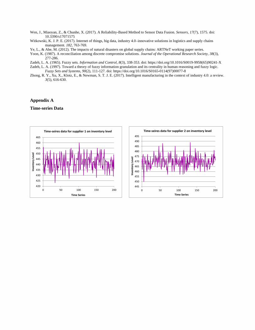
Wen, J., Miaoyan, Z., & Chunhe, X. (2017). A Reliability-Based Method to Sensor Data Fusion. Sensors, 17(7), 1575. doi:

10.3390/s17071575

Witkowski, K. J. P. E. (2017). Internet of things, big data, industry 4.0–innovative solutions in logistics and supply chains

management. 182, 763-769.

Ye, L., & Abe, M. (2012). The impacts of natural disasters on global supply chains: ARTNeT working paper series.

Yoon, K. (1987). A reconciliation among discrete compromise solutions. Journal of the Operational Research Society, 38(3),

277-286.

Zadeh, L. A. (1965). Fuzzy sets. Information and Control, 8(3), 338-353. doi: https://doi.org/10.1016/S0019-9958(65)90241-X

Zadeh, L. A. (1997). Toward a theory of fuzzy information granulation and its centrality in human reasoning and fuzzy logic.

Fuzzy Sets and Systems, 90(2), 111-127. doi: https://doi.org/10.1016/S0165-0114(97)00077-8

Zhong, R. Y., Xu, X., Klotz, E., & Newman, S. T. J. E. (2017). Intelligent manufacturing in the context of industry 4.0: a review.

3(5), 616-630.

Appendix A

Time-series Data

420

425

430

435

440

445

450

455

460

465

0 50 100 150 200

Inve

nto

ry L

eve

l

Time Series

Time-seires data for supplier 1 on inventory level

445

450

455

460

465

470

475

480

485

490

495

0 50 100 150 200

Inve

nto

ry L

eve

l

Time Series

Time-seires data for supplier 2 on inventory level

Figure 15. Time-series data for suppliers on pre-positioned inventory level (𝐶1)

420

425

430

435

440

445

450

455

460

0 50 100 150 200

Inve

nto

ry L

eve

l

Time Series

Time-seires data for supplier 5 on inventory level

420

430

440

450

460

470

480

490

0 50 100 150 200

Inve

nto

ry L

eve

l

Time Series

Time-seires data for supplier 3 on inventory level

390

400

410

420

430

440

450

460

0 50 100 150 200

Inve

nto

ry L

eve

l

Time Series

Time-seires data for supplier 4 on inventory level

Figure 16. Time-series data for suppliers on lead time variability (𝐶2)

7

8

9

10

11

12

13

14

15

16

0 50 100 150 200

De

live

ry T

ime

(D

ay)

Time Series

Time-seires data for supplier 1 on lead time

4

6

8

10

12

14

0 50 100 150 200

De

live

ry T

ime

(D

ay)

Time Series

Time-seires data for supplier 2 on lead time

8

10

12

14

16

18

20

0 50 100 150 200

De

live

ry T

ime

(D

ay)

Time Series

Time-seires data for supplier 3 on lead time

11

12

13

14

15

16

17

0 50 100 150 200

De

live

ry T

ime

(D

ay)

Time Series

Time-seires data for supplier 4 on lead time

5

7

9

11

13

15

17

19

21

0 50 100 150 200

De

live

ry T

ime

(D

ay)

Time Series

Time-seires data for supplier 5 on lead time

Historically collected data presented in graphical format

Figure 17. Graphical information for suppliers on non-time-series attributes

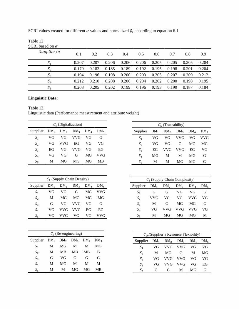
SCRI values created for different 𝛼 values and normalized �̃�𝑖 according to equation 6.1

Table 12

SCRI based on 𝛼

𝑆𝑢𝑝𝑝𝑙𝑖𝑒𝑟/𝛼

0.1 0.2 0.3 0.4 0.5 0.6 0.7 0.8 0.9

𝑆1 0.207 0.207 0.206 0.206 0.206 0.205 0.205 0.205 0.204

𝑆2 0.179 0.182 0.185 0.189 0.192 0.195 0.198 0.201 0.204

𝑆3 0.194 0.196 0.198 0.200 0.203 0.205 0.207 0.209 0.212

𝑆4 0.212 0.210 0.208 0.206 0.204 0.202 0.200 0.198 0.195

𝑆5 0.208 0.205 0.202 0.199 0.196 0.193 0.190 0.187 0.184

Linguistic Data:

Table 13.

Linguistic data (Performance measurement and attribute weight)

𝐶5 (Digitalization)

Supplier DM1 DM2 DM3 DM4 DM5

𝑆1 VG VG VVG VG G

𝑆2 VG VVG EG VG VG

𝑆3 EG VG VVG VG EG

𝑆4 VG VG G MG VVG

𝑆5 M MG MG MG MB

𝐶7 (Supply Chain Density)

Supplier DM1 DM2 DM3 DM4 DM5

𝑆1 VG VG G MG VVG

𝑆2 M MG MG MG MG

𝑆3 G VG VVG VG G

𝑆4 VG VVG VVG EG EG

𝑆5 VG VVG VG VG VVG

𝐶6 (Traceability)

Supplier DM1 DM2 DM3 DM4 DM5

𝑆1 VG VG VVG VG VVG

𝑆2 VG VG G MG MG

𝑆3 EG VVG VVG EG VG

𝑆4 MG M M MG G

𝑆5 M M MG MG G

𝐶8 (Supply Chain Complexity)

Supplier DM1 DM2 DM3 DM4 DM5

𝑆1 G G VG VG G

𝑆2 VVG VG VG VVG VG

𝑆3 M G MG MG G

𝑆4 VG VVG VVG VVG VG

𝑆5 M MG MG MG M

𝐶9 (Re-engineering)

Supplier DM1 DM2 DM3 DM4 DM5

𝑆1 M MG M M MG

𝑆2 M MB MB MB B

𝑆3 G VG G G G

𝑆4 M MG M M M

𝑆5 M M MG MG MB

𝐶10(Supplier’s Resource Flexibility)

Supplier DM1 DM2 DM3 DM4 DM5

𝑆1 VG VVG VVG VG VG

𝑆2 M MG G M MG

𝑆3 VG VVG VVG VG VG

𝑆4 VG VVG VVG VG EG

𝑆5 G G M MG G

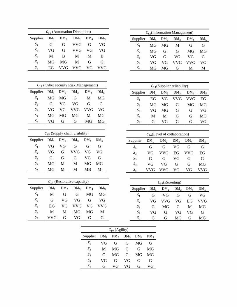
𝐶11 (Automation Disruption)

Supplier DM1 DM2 DM3 DM4 DM5

𝑆1 G G VVG G VG

𝑆2 VG G VVG VG VG

𝑆3 M B M M B

𝑆4 MG MG M G G

𝑆5 EG VVG VVG VG VVG

𝐶12(Information Management)

Supplier DM1 DM2 DM3 DM4 DM5

𝑆1 MG MG M G G

𝑆2 MG G G MG MG

𝑆3 VG G VG VG G

𝑆4 VG VG VVG VVG VG

𝑆5 MG MG G M M

𝐶13 (Cyber security Risk Management)

Supplier DM1 DM2 DM3 DM4 DM5

𝑆1 MG MG G M MG

𝑆2 G VG VG G G

𝑆3 VG VG VVG VVG VG

𝑆4 MG MG MG M MG

𝑆5 VG G G MG MG

𝐶14(Supplier reliability)

Supplier DM1 DM2 DM3 DM4 DM5

𝑆1 EG VG VVG VVG EG

𝑆2 MG MG G MG MG

𝑆3 VG MG G G VG

𝑆4 M M G G MG

𝑆5 G VG G G VG

𝐶15 (Supply chain visibility)

Supplier DM1 DM2 DM3 DM4 DM5

𝑆1 VG VG G G G

𝑆2 VG G VVG VG VG

𝑆3 G G G VG G

𝑆4 MG M M MG MG

𝑆5 MG M M MB M

𝐶16(Level of collaboration)

Supplier DM1 DM2 DM3 DM4 DM5

𝑆1 G G VG G G

𝑆2 VG VVG EG VVG EG

𝑆3 G G VG G G

𝑆4 VG VG G G MG

𝑆5 VVG VVG VG VG VVG

𝐶17 (Restorative capacity)

Supplier DM1 DM2 DM3 DM4 DM5

𝑆1 M G G MG MG

𝑆2 G VG VG G VG

𝑆3 EG VG VVG VG VVG

𝑆4 M M MG MG M

𝑆5 VVG G VG G G

𝐶18(Rerouting)

Supplier DM1 DM2 DM3 DM4 DM5

𝑆1 G VG G G VG

𝑆2 VG VVG VG EG VVG

𝑆3 G MG G M MG

𝑆4 VG G VG VG G

𝑆5 G G MG G MG

𝐶19 (Agility)

Supplier DM1 DM2 DM3 DM4 DM5

𝑆1 VG G G MG G

𝑆2 M MG G G MG

𝑆3 G MG G MG MG

𝑆4 VG G VG G G

𝑆5 G VG VG G VG

Table 14.

Linguistic terms (used in performance measurement)

and coresponding TFNs

Weight of the attribute

Attribute DM1 DM2 DM3 DM4 DM5

𝐶1 I VI EI I VI

𝐶2 M I VI I M

𝐶3 M M I M I

𝐶4 I I VI I I

𝐶5 I I VI VI I

𝐶6 EI I EI EI I

𝐶7 M M I I M

𝐶8 I VI I I VI

𝐶9 M UI M M UI

𝐶10 I VI VI VI I 𝐶11 I I VI VI I 𝐶12 I MI MI I MI 𝐶13 M MI I MI I 𝐶14 VI I I VI VI 𝐶15 MI I M MI M

𝐶16 I VI VI MI I 𝐶17 I M M VI I 𝐶18 I I MI M MI 𝐶19 M MI I MI MI

Performance Measurement

Linguistic Terms TFN (a, b, c)

VB (0,1,2)

B (1,2,3)

… …

EG (8,9,10)

Appendix B

Attributes concerning time series data

Based on the approach described in sub-step 1(a) and the original time-series data in Figure 15 and Figure

16, the possibility distribution in the form of triangular fuzzy number are generated as follows:

Figure 18. Graphical Triangular Fuzzy Number for suppliers on pre-positioned inventory level (𝐶1)

0

0.2

0.4

0.6

0.8

1

1.2

440 450 460 470 480

Supplier 3

0

0.2

0.4

0.6

0.8

1

1.2

400 420 440 460

Supplier 4

0

0.2

0.4

0.6

0.8

1

1.2

420 430 440 450 460

Supplier 1

0

0.2

0.4

0.6

0.8

1

1.2

450 460 470 480 490

Supplier 2

0

0.2

0.4

0.6

0.8

1

1.2

420 430 440 450 460

Supplier 5

Figure 19. Graphical Triangular Fuzzy Number for suppliers on lead time variability (𝐶2)

With the obtained graphical TFN, the numerical TFN could be constructed from Figure 18 and Figure 19

as:

Table 15.

Numerical Triangular Fuzzy Number for suppliers on 𝐶1 and 𝐶2

Supplier C1 (Pre-positioned Inventory Level) C2 (Lead Time Variability)

a b c a b c

𝑆1 423.98 441.04 454 7.98 11.01 15

𝑆2 459.98 469.54 480 5.98 9 12

𝑆3 441.98 455.01 470 10.98 14.03 17

𝑆4 404.98 425.51 445 11.98 14.01 16

𝑆5 424.98 446.05 459 9.98 14 18

0

0.2

0.4

0.6

0.8

1

1.2

0 5 10 15 20

Supplier 1

0

0.2

0.4

0.6

0.8

1

1.2

0 5 10 15

Supplier 2

0

0.2

0.4

0.6

0.8

1

1.2

0 5 10 15 20

Supplier 3

0

0.2

0.4

0.6

0.8

1

1.2

0 5 10 15 20

Supplier 4

0

0.2

0.4

0.6

0.8

1

1.2

0 5 10 15 20

Supplier 5

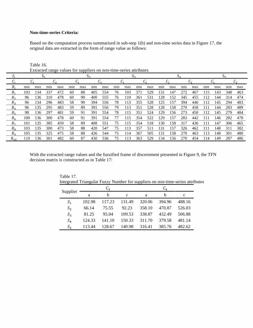
Non-time-series Criteria:

Based on the computation process summarized in sub-step 1(b) and non-time series data in Figure 17, the

original data are extracted in the form of range value as follows:

Table 16.

Extracted range values for suppliers on non-time-series attributes

𝑆𝑖 S1 S2 S3 S4 S5

𝐶𝑖 𝐶1 𝐶2 𝐶1 𝐶2 𝐶1 𝐶2 𝐶1 𝐶2 𝐶1 𝐶2

𝑅𝑖 min max min max min max min max min max min max min max min max min max min max

𝑅1 103 134 337 472 60 88 405 554 76 103 371 529 131 147 272 467 115 143 348 463

𝑅2 96 136 310 478 60 90 400 555 76 110 361 531 128 152 345 455 112 144 314 474

𝑅3 96 134 296 483 58 90 394 556 78 113 355 528 125 157 394 446 112 145 294 483

𝑅4 96 135 295 483 59 89 391 556 79 113 351 528 128 158 270 458 111 144 283 489

𝑅5 98 136 297 481 59 91 391 554 78 115 351 524 129 156 273 450 112 145 279 484

𝑅6 100 136 300 478 60 91 391 554 77 115 354 522 129 157 283 442 111 146 282 478

𝑅7 101 135 385 459 58 89 408 551 75 115 354 518 130 158 317 436 111 147 306 465

𝑅8 103 135 300 473 58 88 420 547 75 113 357 511 131 157 326 462 111 148 311 382

𝑅9 105 135 325 475 58 88 426 544 75 114 367 505 131 158 270 463 113 148 301 480

𝑅10 110 136 301 482 60 87 430 536 75 113 363 529 134 156 270 454 114 149 287 486

With the extracted range values and the fuzzified frame of discernment presented in Figure 9, the TFN

decision matrix is constructed as in Table 17:

Table 17.

Integrated Triangular Fuzzy Number for suppliers on non-time-series attributes

Supplier 𝐶3 𝐶4

a b c a b c

𝑆1 102.98 117.23 131.49 320.06 394.96 488.16

𝑆2 66.14 75.55 92.23 358.10 470.87 526.03

𝑆3 81.25 95.04 109.53 338.87 432.49 506.88

𝑆4 124.33 141.10 150.33 311.70 379.58 481.14

𝑆5 113.44 128.67 140.98 316.41 385.76 482.62

According to sub-step 2(b) and Table 13, the attribute weight decision matrix is constructed as:

Table 18.

Attribute weight decision matrix

Attribute Weight

a b c

𝐶1 0.5 0.7 1

𝐶2 0.3 0.54 0.8

𝐶3 0.3 0.48 0.7

𝐶4 0.5 0.62 0.8

𝐶5 0.5 0.64 0.8

𝐶6 0.5 0.78 1

𝐶7 0.3 0.48 0.7

𝐶8 0.5 0.64 0.8

𝐶9 0.1 0.32 0.5

𝐶10 0.5 0.66 0.8

𝐶11 0.5 0.64 0.8

𝐶12 0.4 0.54 0.7

𝐶13 0.3 0.52 0.7

𝐶14 0.5 0.66 0.8

𝐶15 0.3 0.48 0.7

𝐶16 0.4 0.62 0.8

𝐶17 0.3 0.54 0.8

𝐶18 0.3 0.52 0.7

𝐶19 0.3 0.5 0.7

The PIS and NIS matrix are generated based on function (5.6) and (5.7) in step 3:

Table 19.

PIS and NIS for attributes

Attribute PIS NIS

TFN a b c a b c

𝐶1 1.00 1.00 1.00 0.42 0.42 0.42

𝐶2 0.80 0.80 0.80 0.10 0.10 0.10

𝐶3 0.70 0.70 0.70 0.06 0.06 0.06

𝐶4 0.80 0.80 0.80 0.15 0.15 0.15

𝐶5 0.80 0.80 0.80 0.22 0.22 0.22

𝐶6 1.00 1.00 1.00 0.30 0.30 0.30

𝐶7 0.70 0.70 0.70 0.09 0.09 0.09

𝐶8 0.80 0.80 0.80 0.17 0.17 0.17

𝐶9 0.50 0.50 0.50 0.01 0.01 0.01

𝐶10 0.80 0.80 0.80 0.15 0.15 0.15

𝐶11 0.80 0.80 0.80 0.05 0.05 0.05

𝐶12 0.70 0.70 0.70 0.13 0.13 0.13

𝐶13 0.70 0.70 0.70 0.10 0.10 0.10

𝐶14 0.80 0.80 0.80 0.15 0.15 0.15

𝐶15 0.70 0.70 0.70 0.07 0.07 0.07

𝐶16 0.80 0.80 0.80 0.16 0.16 0.16

𝐶17 0.80 0.80 0.80 0.09 0.09 0.09

𝐶18 0.70 0.70 0.70 0.09 0.09 0.09

𝐶19 0.7 0.7 0.7 0.11 0.11 0.11