resistance factors for 100% dynamic testing, with and

Final Report

FDOT Contract No.: BDK-75-977-25

UF Contract No.: 00083426

Resistance Factors for 100% Dynamic Testing, With and Without Static Load Tests

Principal Investigators: Michael C. McVay

Harald Klammler

Department of Civil and Coastal Engineering University of Florida

Gainesville, Florida 32611-6580

Developed for the

Rodrigo Herrera, P.E., Project Manager Peter Lai, P.E., Co-Project Manager

May 2011

ii

DISCLAIMER

The opinions, findings, and conclusions expressed in this

publication are those of the authors and not necessarily

those of the Florida Department of Transportation or the

U.S. Department of Transportation.

Prepared in cooperation with the State of Florida Depart-

ment of Transportation and the U.S. Department of

Transportation.

iii

SI (MODERN METRIC) CONVERSION FACTORS (from FHWA)

APPROXIMATE CONVERSIONS TO SI UNITS

SYMBOL WHEN YOU KNOW MULTIPLY BY TO FIND SYMBOL

LENGTH

in inches 25.4 millimeters mm

ft feet 0.305 meters m

yd yards 0.914 meters m

mi miles 1.61 kilometers km


AREA

in2 square inches 645.2 square millimeters mm2

ft2 square feet 0.093 square meters m2

yd2 square yard 0.836 square meters m2

ac acres 0.405 hectares ha

mi2 square miles 2.59 square kilometers km2


VOLUME

fl oz fluid ounces 29.57 milliliters mL

gal gallons 3.785 liters L

ft3 cubic feet 0.028 cubic meters m3

yd3 cubic yards 0.765 cubic meters m3

NOTE: volumes greater than 1000 L shall be shown in m3


MASS

oz ounces 28.35 grams g

lb pounds 0.454 kilograms kg

T short tons (2000 lb) 0.907 megagrams (or "metric ton")

Mg (or "t")


TEMPERATURE (exact degrees)

°F Fahrenheit 5 (F-32)/9 or (F-32)/1.8

Celsius °C


ILLUMINATION

fc foot-candles 10.76 lux lx

fl foot-Lamberts 3.426 candela/m2 cd/m2


FORCE and PRESSURE or STRESS

Lbf * poundforce 4.45 newtons N

kip kip force 1000 pounds lbf

lbf/in2 poundforce per square inch 6.89 kilopascals kPa

iv

APPROXIMATE CONVERSIONS TO SI UNITS


LENGTH

mm millimeters 0.039 inches in

m meters 3.28 feet ft

m meters 1.09 yards yd

km kilometers 0.621 miles mi


AREA

mm2 square millimeters 0.0016 square inches in2

m2 square meters 10.764 square feet ft2

m2 square meters 1.195 square yards yd2

ha hectares 2.47 acres ac

km2 square kilometers 0.386 square miles mi2


VOLUME

mL milliliters 0.034 fluid ounces fl oz

L liters 0.264 gallons gal

m3 cubic meters 35.314 cubic feet ft3

m3 cubic meters 1.307 cubic yards yd3


MASS

g grams 0.035 ounces oz

kg kilograms 2.202 pounds lb

Mg (or "t") megagrams (or "metric ton") 1.103 short tons (2000 lb) T


TEMPERATURE (exact degrees)

°C Celsius 1.8C+32 Fahrenheit °F


ILLUMINATION

lx lux 0.0929 foot-candles fc

cd/m2 candela/m2 0.2919 foot-Lamberts fl


FORCE and PRESSURE or STRESS

N newtons 0.225 poundforce lbf

kPa kilopascals 0.145 poundforce per square inch

lbf/in2

*SI is the symbol for International System of Units. Appropriate rounding should be made to comply with Section 4 of ASTM E380. (Revised March 2003)

v

TECHNICAL REPORT DOCUMENTATION PAGE 1. Report No.

2. Government Accession No.

3. Recipient's Catalog No.

4. Title and Subtitle

Resistance Factors for 100% Dynamic Testing,

With and Without Static Load Tests

5. Report Date

May 2011

6. Performing Organization Code

7. Author(s)

Michael McVay and Harald Klammler

8. Performing Organization Report No.

UF Project 00083426

9. Performing Organization Name and Address

Department of Civil and Coastal Engineering 365 Weil Hall – P.O. Box 116580 University of Florida Gainesville, FL 32611-6580

10. Work Unit No. (TRAIS)

11. Contract or Grant No.

BDK-75-977-25

12. Sponsoring Agency Name and Address

Florida Department of Transportation 605 Suwannee Street, MS 30 Tallahassee, FL 32399

13. Type of Report and Period Covered

Final Report 09/24/09 - 06/30/11

14. Sponsoring Agency Code

15. Supplementary Notes

16. Abstract

Current department of transportation (DOT) and Federal Highway Administration (FHWA) practice has highly variable load and resistance factor design (LRFD) resistance factors, , for driven piles from design (e.g., Standard Penetration Tests (SPT), Cone Penetrometer Test (CPT)) to construction (e.g., pile monitoring). Complicating the construction effort, are the number of piles monitored (e.g., 10% versus 100%), as well as the type of monitoring (e.g., high strain rate: Embedded Data Collector (EDC), Pile Driving Analyzer (PDA), static load test, etc.). Of great interest are quantifying the influence of number of piles within a group, number of piles monitored, as well as spatial variability on a pile group’s uncertainty and associated LRFD factors.

The work startedwith an investigation of probability of failure (POF) of a bridge in terms of its piers and underlying piles. It was discovered that the number of piles in a pier may have a large impact on POF of a pier, which is why the development of LRFD Φ should occur with respect to pier (i.e., pile group) level and include the total number of piles within the group as well as the distribution of monitored and unmonitored piles within the group. Next, the total uncertainty of the pier including spatial variability and error of the method (e.g., SPT, EDC/PDA, etc.) was investigated. The work started with spatial uncertainty of single pile resistance (side plus tip) from SPT data and then extended through kriging (considering different weights for individual borings) to group layouts (e.g., double, triple, quads, etc.) for assessing group resistance uncertainty, CVR. Subsequently, the kriging group work was carried over to assessing uncertainty, i.e., spatial and method error (predicted versus static load test) for high strain rate field measurements. Equations and charts were developed to quantify group uncertainty, CVR, and LRFD for typical group layouts and monitoring. The latter approach was considered to be inflexible, and the spatial uncertainty (i.e., kriging) was replaced with hammer monitoring in conjunction with high strain rate monitoring. Using the uncertainty of monitoring method (CVm) and a measured uncertainty of blow count regression (CVεh) versus high strain rate monitoring, an LRFD equation was developed for pile groups considering the numbers of monitored and unmonitored piles. The developed expression was evaluated at two sites and gave reasonable predictions compared to current practice.

17. Key Words

LRFD , pile monitoring, pile groups, EDC, PDA, and CAPWAP

18. Distribution Statement

No restrictions.

19. Security Classif. (of this report)

Unclassified 20. Security Classif. (of this page)

Unclassified 21. No. of Pages

105 22. Price

Form DOT F 1700.7 (8-72) Reproduction of completed page authorized

vi

EXECUTIVE SUMMARY

The departments of transportation (DOTs) and the Federal Highway Administration

(FHWA) have moved away from an allowable stress design (ASD) to a load and resistance

factor design (LRFD) based on probability of failure for deep foundations. In the case of driven

piles, LRFD factors vary significantly from design methods (e.g., American Association of

State Highway and Transportation Officials (AASHTO, 2004): Standard Penetration Test (SPT):

=0.45) to construction monitoring ( = 0.65 — Pile Driving Analyzer (PDA), Embedded

Data Collector (EDC)). Complicating the construction effort, are the number of piles monitored

(e.g., 10% versus 100%), as well as the type of monitoring (e.g., high strain rate: EDC, PDA;

static load test, etc.). Of great interest are quantifying the influence of number of piles within a

group, number of piles monitored, as well as spatial variability, on a pile group’s resistance

uncertainty and associated LRFD factors.

The effort started with a discussion of probability of failure (POF) of a bridge and defines

failure in terms of redundant and non-redundant systems. It was found that the number of piles

in a pier may have a large impact on POF at the pier level. Therefore, it was decided to establish

the LRFD Φ based on the POF of the whole pier which includes the total number of piles within

the group as well as the distribution of monitored and unmonitored piles within the group.

Next, to establish an LRFD , total uncertainty — which included spatial variability (i.e.,

monitored versus unmonitored) and method error (e.g., SPT, EDC/PDA versus static load test)

— was investigated. The work started with spatial group uncertainty of a single pile resistance

(side plus tip) from SPT data and was then extended through kriging (considering different

weights for adjacent borings) to group layouts (e.g., double, triple, quads, etc.) to assess group

uncertainty CVR. Subsequently, the kriging group work was carried over to assessing

vii

uncertainty, i.e., spatial and method error (predicted versus static load test) for high strain rate

field measurements. The effort developed charts identifying the uncertainty (variance) reduction

(e) for a specific group based on number and geometric configuration of piles monitored within

a group, total piles within the group, and number of pile groups at the site. Unfortunately, no

simple analytical expression for variance reduction in terms of pile group layouts could be

developed and the approach had limited flexibility in the sense of assuming all piles had similar

embedment depths or blow counts (i.e., also similar resistances) and the group design load was

unknown apriori.

To overcome these problems associated with the spatial uncertainty, the use of hammer

blow count data in combination with high strain rate measurements was introduced to assess a

pile group’s resistance uncertainty. Generally, good correlations were observed with static

capacity by using Federal Highway Administration (FHWA) Gates dynamic formula

(Paikowsky, 2004) or high strain rate test assessments. As with prior work, the uncertainty of

the pile group was expressed in terms of the uncertainties of monitored (CVεm: high strain rate

data: EDC, PDA, etc.) and unmonitored piles (hammer blow count measurements). In terms of

the unmonitored piles within a group, their uncertainty (CVεh) was assessed by linear correlation

between blow count data and EDC/PDA capacities. Subsequently, the total group resistance Rg,

and its associated uncertainty in terms of the coefficient of variation CVR, was assessed. Using

the group uncertainty CVR with a representative reliability of the group (e.g., = 3), a relatively

simple LRFD expression was developed for a driven pile group depending on number of

monitored and unmonitored piles in the group, and uncertainty of monitoring method (CVm) as

well as uncertainty of blow count regression (CVεh). The applicability of the developed LRFD

expression was evaluated on two separate sites with driven prestressed concrete piles.

Interestingly, full monitoring gave LRFD values similar to literature (i.e., AASHTO, 2009,

viii

Florida Department of Transportation, 2009); however of great importance and not reported in

the literature is the influence of pile group size and uncertainty of monitoring approach (i.e.,

CVεm, and CVεh). Finally, the proposed expression will allow different considerations, such as

different degrees of method uncertainties (e.g., due to employing end of drive (EOD) versus

beginning of redrive (BOR): variability of pile capacities; equipment, as well as site and soil

conditions.

ix

TABLE OF CONTENTS page EXECUTIVE SUMMARY ..................................................................................................... vi LIST OF TABLES ................................................................................................................... xi LIST OF FIGURES ................................................................................................................ xii CHAPTERS 1 INTRODUCTION ...................................................................................................1 1.1 Background .....................................................................................................1 1.2 Scope of Research ...........................................................................................3 2 GENERAL ASPECTS OF DEEP FOUNDATION RELIABILITY

ASSESSMENT ........................................................................................................4 2.1 Estimation Bias and Uncertainty ....................................................................4 2.2 Probability of Failure ......................................................................................6 3 SPATIAL UNCERTAINTY OF FB-DEEP SPT/CPT CAPACITY ASSESSMENT .................................................................................11 3.1 Background ...................................................................................................11 3.2 Theory ...........................................................................................................11 3.3 Example of FB-Deep Spatial Uncertainty of a Pile/shaft in Sands ..............19 4 PILE GROUP SPATIAL UNCERTAINTY WITH NEARBY SPT/CPT DATA ...................................................................................23 4.1 Background ...................................................................................................23 4.2 Notation.........................................................................................................23 4.3 Multiple Shaft Foundations without Conditioning Data ...............................24 4.4 Single and Multiple Shaft Foundations with Conditioning Data ..................31 4.5 Discussion of Results ....................................................................................38 4.6 Practical Example .........................................................................................40 5 UNMONITORED, PARTIALLY AND FULLY MONITORED PILE

GROUPS – KRIGING APPROACH.....................................................................44 5.1 Background ...................................................................................................44 5.2 List of Variables for Chapter Five ................................................................44 5.3 Predicting Pile Group Resistance from Monitored Piles Using Kriging .......................................................................................46 5.4 Discussion of Results ....................................................................................54 5.4.1 No Pile Monitored in Group of Interest (nm1 = 0) .............................54 5.4.2 One Pile Monitored in Group of Interest (nm1 = 1) ...........................54 5.4.3 All Piles Monitored in Group of Interest (nm1 = np1) ........................55 5.4.4 Single Pile Group without Spatial Correlation (ng = 1 and ah = 0) ...56

x

5.5 Worst Case Scenarios of Unknown ah ..........................................................56 5.6 Practical Example .........................................................................................63 6 UNMONITORED, PARTIALLY AND FULLY MONITORED PILE GROUPS – REGRESSION APPROACH .............................................................65 6.1 Background ...................................................................................................65 6.2 Examples of Relationships between Blow Count and Pile Capacities ...............................................................................................66 6.3 List of Variables for Chapter 6 .....................................................................69 6.4 The Regression Approach .............................................................................70 6.5 Practical Example .........................................................................................76 7 SUMMARY AND CONCLUSIONS ....................................................................82 REFERENCES ........................................................................................................................87 APPENDIX A – SPATIAL CORRELATION VERSUS COLLOCATED SECONDARY DATA ......................................................88

xi

LIST OF TABLES Table page 1-1 AASHTO 10.5.5.2.3-1 (2009) ....................................................................................2 5-1 Summary of Results from Practical Example ...........................................................64 6-1 Summary Statistics for ENR and FHWA-Modified Gates .......................................68

xii

LIST OF FIGURES Figure page 2-1 Scatterplots of predicted values: (a) before bias correction P; and (b)after

bias correction P versus true values T .......................................................................5 2-2 Probability of failure (POF) versus reliability index ..............................................6 2-3 Contour lines of log10(pb) as a function of pℓ , nℓ, and nr from Equation 2.5 ..........9 3-1 Schematic of driven pile (circular or square) with SPT or CPT data

available along center line (dashed) for use in FB-Deep method ...........................12 3-2 Illustration of how the double integral in A may be converted into a single integral using the frequency of occurrence of location pairs

on Lab, which are separated by distance h ...............................................................17 3-3 Illustration of how the double integral in B may be converted into a single integral using the frequency of occurrence of location pairs between Lab and Lbc, which are separated by distance h .........................................18 3-4 1/2 from Equation 3.22 for exponential covariance function (Equation 3.16). ......21 3-5 1/2 from Equation 3.22 (continuous) and its rational approximation from

Equation 3.24 (dashed) valid for L/av > 1.5 ............................................................21 3-6 1/2 from numerical integration of Equation 3.11 for spherical covariance

function (Equation 3.15) ..........................................................................................22 3-7 1/2 from numerical integration of Equation 3.11 (continuous) and a rational

approximation as 1.07 times from Equation 3.24 (dashed) .................................22 4-1 (a) Example of quadruple “Q” square configuration with (b) respective shaft

separation matrix in multiples of D, and (c) and (d) are variance–covariance matrices in multiples of the upscaled single shaft variance 2

s ...............................27

4-2 Further examples of multiple shaft configurations with rigid pile caps and

possible center borings (crosses) .............................................................................28 4-3 1/ 2

qf as a function of L/av for single and multiple shaft configurations of Figures

4-1 and 4-2 with Ds /D = 3 .......................................................................................29 4-4 Typical plan view of borehole (crosses) and foundation locations (e.g.,

quadruple shaft foundation for a bridge site) ..........................................................31

xiii

4-5 The term r = Cbf (0)/Cb(0) as a function of ah/D for L/av > 1 (continuous), L/av = 0 (dashed) and different shaft configurations (Ds = 3D) ..............................35

4-6 Performance of different shaft configurations under the worst case scenario

of Equations 21 and 22 for unknown ah in the presence of a center boring ............37 4-7 Worst case scenarios for example problem and different values of qb1/qbm ............42 5-1 Examples of an (a) 3 3 (npi = 9) and a (b) 4 4 (npi = 16) pile group with

monitoring configurations (black circles) and pile numbering using index j ..........47 5-2 (a) Example of pile groups and monitoring configurations (black

circles) for ng = 4; (b) Simplified model corresponding to Equation 5.9 ................48 5-3 Difference between Cε (h) and C(h). .......................................................................50 5-4 Variance–covariance matrix between all piles of the example in Figure 5-1a

(npi = 9 and nmi = 4) .................................................................................................52 5-5 Terms W1 (dashed, except for (a), where W1 does not exist as no pil is

monitored in the group) and e (continuous) as functions of ah /Ds from Equations 5.14 and 5.15 for a double pile group .....................................................57

5-6 Analogous to Figure 5-5 for tripe pile groups in a line and different

monitoring configurations .......................................................................................58 5-7 Analogous to Figure 5-5 for tripe pile groups in a triangle and different

monitoring configurations .......................................................................................59 5-8 Analogous to Figure 5-5 for 2 2 pile groups and different monitoring

configurations ..........................................................................................................60 5-9 Analogous to Figure 5-5 for 3 3 pile groups and different monitoring

configurations ..........................................................................................................61 5-10 Analogous to Figure 5-5 for 4 4 pile groups and different monitoring

configurations ..........................................................................................................61 6-1 Comparison of ENR and FHWA-Gates for Delmag D22 .......................................67 6-2 Example data from driving of a single pile (pile 7) at Caminida: (a) Depth

profiles of monitored resistance Rm and blow count Nh; (b) Scatter plot and linear regression between Nh and Rm; and (c) Scatter plot and linear regression between ln(Nh) and ln(Rm) .......................................................................................71

xiv

6-3 Term Φ (with λR = 1 and for β = {2, 2.5, 3, 3.5, 4}) as a function of CVg from

full AASHTO equation (black) and linear approximations (red) from Equation 6.8 for the range CVg ≥ 0.05, Φ > 0.4 and 2 ≤ β ≤ 4 ...............................................73

6-4 Depth profiles of monitored resistances Rm and blow counts Nh for:

(a) Caminida pile 1; (b) Dixie pile 1; and (c) Dixie pile 7 ......................................77 6-5 Combined scatter plots and linear regression fits of monitored resistance Rm

versus blow count Nh data from Caminida piles 1 + 8 and Dixie piles 1 + 7: (a) Raw data; and (b) log-transformed data .............................................................78

6-6 LRFD as a function of degree of monitoring for different numbers of piles in

a group (see legend) using CVm = 0.25, CVh = 0.48 and = 3. (a) = f (nm) and (b) = f(nm/np) ................................................................................................79

6-7 Term as a function of degree of monitoring nm /np for np = {4, 9, 16} and

CVh = {0.30, 0.48, 0.80} ........................................................................................80 A-1 Cmm (top curve) and Cmh = Chh =

2mh mmC (bottom curve) ........................................88

A-2 w1/w2 as a function of mh and s .............................................................................91

1

CHAPTER 1 INTRODUCTION

1.1 Background

The recommended load and resistance factor design (LRFD) Φ factor for the design of

driven piles using in situ Standard Penetration Tests (SPT) varies from 0.35 to 0.45 (e.g.,

AASHTO Table 10.5.5.2.3-1 –Tomlinson versus Meyerhof). The value of Φ is a combination of

uncertainty of design methods (i.e., Tomlinson versus Meyerhof) and number of borings as well

as their locations relative to the pile. In the case of high strain rate field monitoring (e.g., Pile

Driving Analyzer (PDA), Embedded Data Collector (EDC)), LRFD Φ factor increases to 0.65

according to FDOT Structures Design Guidelines if PDA and CAPWAP are used for approxi-

mately 10% of the piles during driving. In general, increasing LRFD Φ from 0.45 to 0.65 could

potentially result in a 40% saving in pile length cost in uniform soil deposit without

consideration of reduced driving times, equipment needs (e.g., bigger crane for longer piles), etc.

Recently, the Florida Department of Transportation (FDOT) funded the development of

wireless pile monitoring, i.e., EDC, focusing on reducing pile monitoring cost/time and

improved safety. Specifically, the technology uses: 1) wireless communication, which

eliminates the need for personnel to climb (safety) pile leads (in some instances > 80 ft.) for gage

attachment to the pile; 2)dual location of the instrumentation, which improves the “real time”

assessment of dynamic stresses (e.g., pile damage during hard driving), static tip resistance (end

bearing piles) for every hammer blow, as well as separation of side from tip resistance

(dynamically and statically); and finally, 3)the wireless system, the instrumentation of which

uses technologies developed for other mass markets (e.g., automotive, ITT, etc.) leading

potentially to a larger number of monitored piles, e.g., 100% .

2

Of great interest is the appropriate LRFD Φ resistance value based on the number of piles

monitored within a group. Obviously, monitoring every pile should increase Φ, but if the predic-

tion method is non-conservative (e.g., biased) LRFD Φ should be less than one, whereas, for a

conservative method Φ may be greater than one. In addition, if the designer/contractor decides

to monitor just 50% of the piles, what are the recommended LRFD Φ factors given the soil/rock

strength variability (coefficient of variation CV and spatial correlation, i.e., covariance)?

Current design practices suggested by AASHTO (2009) (Table 1-1) use pre-defined values

of Φ depending on number of piles monitored, type of monitoring, and whether static load

testing is performed. For example, Φ = 0.75 if all piles are monitored and Φ = 0.80 if 2% of the

piles are monitored plus one static load test is performed. The table does consider older moni-

toring approaches (e.g., Gates, Φ = 0.40) based on hammer energy and measured blow counts.

Evidently, all of the approaches do not explicitly account for the spatial heterogeneity that gener-

ally exists between individual piles (monitored and unmonitored) in a group, number of piles

Table 1-1. AASHTO 10.5.5.2.3-1 (2009)

Condition/Resistance Determination Method Resistance

Factor

Nominal bearing resistance of single pile–dynamic analysis and static load test method

Driving criteria established by successful static load test of at least one pile per site condition and dynamic testing of at least two piles per site condition, but no less than 2% of the production piles

0.8

Driving criteria established by successful static load test of at least one pile per site condition without dynamic testing

0.75

Driving criteria established by dynamic testing conducted on 100% of production piles

0.75

Driving criteria established by dynamic test with signal matching at beginning of redrive (BOR) conditions only of at least one product pile per pier, but no less than the number of tests provided in Table 10.5.5.2.3-3

0.65

Wave equation analysis, without pile dynamic measurements or load test, at end of drive (EOD) conditions only

0.4

Federal Highway Administration (FHWA)-modified Gates dynamic pile formula (EOD conditions only)

0.4

Engineering News-Record (as defined in Article 10.7.3.8.5) dynamic pile formula (EOD condition only)

0.1

3

monitored within a group, and if combined methods were used (i.e., high strain rate with hammer

blow counts, etc.). Also, due to the typical dimensions of driven piles and expected vertical

loads, piles are generally combined in a group underneath a rigid pile cap to form a foundation.

For such a pile group foundation, if there are none, some, or all individual piles monitored, it will

result in different pile group resistance uncertainties and, hence, different design LRFD

resistance factors Φ of the group. Typically, the larger the number of piles monitored, the

smaller the coefficient of variation of group resistance CVR, thus leading to higher Φ for the

group.

1.2 Scope of Research

The present work attempts to address the shortcomings of current assessment of LRFD Φ

during construction by exploring a geostatistical approach, as well as combining monitored data

with secondary information such as Standard Penetration Test / Cone Penetrometer Test

(SPT/CPT) or hammer blow count data. In what follows, a brief discussion will be given on the

general aspects of measurement bias and uncertainty as well as the probability of failure

(reliability), the latter being perhaps the most fundamental parameter in reliability based design

(Chapter 2). The work then proceeds to an investigation of the uncertainty of single driven pile

resistances based on SPT/CPT data and the FB-Deep design method (Chapter 3). Further,

geospatial kriging approaches are presented for pile groups with nearby SPT/CPT data (Chapter

4) and for partially or fully monitored pile groups (Chapter 5). Finally, the work focuses on

correlation between monitored pile resistances and hammer blow count data. The latter is found

to significantly simplify the geospatial approach and make it more flexible in the sense that less

restrictive assumptions are required (Chapter 6). Although different chapters are related to each

other and a consistent nomenclature is used, deviations may occur and all variables are defined in

their respective chapters.

4

CHAPTER 2 GENERAL ASPECTS OF DEEP FOUNDATION

RELIABILITY ASSESSMENT

2.1 Estimation Bias and Uncertainty

Ideally, pile resistance measurements would be obtained from static load tests on each and

every pile, as they represent a direct replication of pile behavior under service with sufficiently

non-transient (e.g., excluding impact loads) conditions. The static load test measurements are

generally considered as the “true” values. However, static load tests are costly and time-

consuming. Consequently, faster and cheaper methods (SPT/CPT, EDC, PDA, etc.) have been

developed to predict the resistance measured in a top down static load test. Any prediction

method may be biased as well as imprecise, i.e., contain uncertainty. Bias generally refers to

systematic errors between the predictor and true measure (e.g., load test) which remain after unit

conversion (e.g., from SPT blow counts to resistance) and may be corrected for by a

deterministic relationship (i.e., a formula). Imprecision or uncertainty of the method relates to a

random prediction error (variance 2) which remains after bias correction and is due to purely

random components of the measurement process (e.g., instrument errors, imperfections in pile

geometry, etc.).

A bias correction formula applied after unit conversion is equivalent to improving

(correcting) the unit conversion formula itself. Figure 2-1 shows scatterplots of predicted values

(a) before bias correction P and (b) after bias correction P versus true values T. It may be seen

that P is a good predictor of T in the sense that the prediction error ε = P T is zero on average.

The residual scatter of the data points about the 45° line represents the random prediction error

(uncertainty) and is described by the variance 2 of the residuals ε.

5

Figure 2-1. Scatterplots of predicted values: (a) before bias correction P; and (b) after bias

correction P versus true values T.

From this it is seen that “bias correction” is equivalent to finding the relationship between

P and P (e.g., P = a + b P , P = ln(P ), etc.) as indicated in Figure 2-1. For this purpose, both

the type of relationship (e.g., linear, logarithmic, etc.) as well as its coefficients (e.g., a and b)

need to be investigated. Once P is known, 2 is obtained as the variance of the random

prediction error (ε = P – T ) distribution. The random prediction error 2 may be a constant or

depend on T; for example, if σε is directly proportional to T, then the coefficient of variation of

error (CVε = σε,/ = standard deviation divided by mean) is a constant.

Note that different bias relationships may apply to different combinations of prediction

method, construction methods, and soil conditions. Sufficient predicted versus true data pairs are

required to define bias relationships and values of 2 for the largest possible number of

prediction-construction-soil scenarios. Once bias is corrected for, P is known to be equal to T

except for some random error of variance 2 which allows for subsequent (geo-) statistical

treatment.

(b)

45° P

T

(a)

P

T

P = f(P )

6

2.2. Probability of Failure

The probability of failure (POF) and reliability index β are related by definition through

the normal cumulative distribution function as illustrated in Figure 2-2.

1 1.5 2 2.5 3 3.5 4 4.5 5-7

-6

-5

-4

-3

-2

-1

0

[-]

log 1

0(p

of)

[-]

Figure 2-2. Probability of failure (POF) versus reliability index β. Here, pf = G(β) where G() is the normal cumulative distribution function.

The POF pb of a whole bridge is determined by the POFs and the level of redundancy of its

individual components. Limiting our attention to foundation failure only (i.e., not considering

failure of other structural bridge components), then pb becomes a mere function of the individual

POFs pri of each of its nr piers. The level of redundancy expresses how many piers must

simultaneously fail in order to cause the whole bridge to fail. Full redundancy means that all

piers must fail for the bridge to fail; this is not a reasonable assumption for bridges, but may be

so for other structures. For such a case,

1

r rn n

b ri rip p p

(2.1)

7

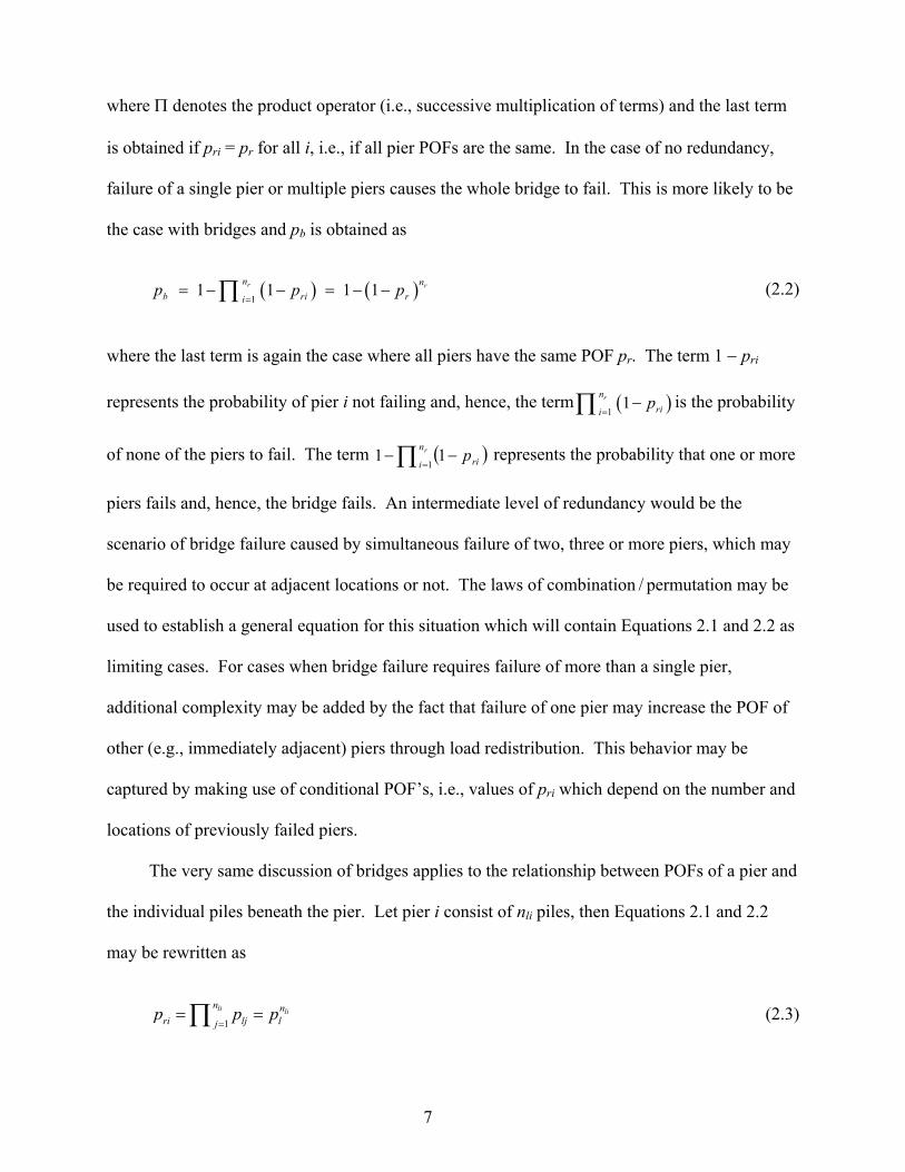
where denotes the product operator (i.e., successive multiplication of terms) and the last term

is obtained if pri = pr for all i, i.e., if all pier POFs are the same. In the case of no redundancy,

failure of a single pier or multiple piers causes the whole bridge to fail. This is more likely to be

the case with bridges and pb is obtained as

1

1 1 1 1r rn n

b ri rip p p

(2.2)

where the last term is again the case where all piers have the same POF pr. The term 1 pri

represents the probability of pier i not failing and, hence, the term 1

1rn

riip

is the probability

of none of the piers to fail. The term rn

i rip1

11 represents the probability that one or more

piers fails and, hence, the bridge fails. An intermediate level of redundancy would be the

scenario of bridge failure caused by simultaneous failure of two, three or more piers, which may

be required to occur at adjacent locations or not. The laws of combination / permutation may be

used to establish a general equation for this situation which will contain Equations 2.1 and 2.2 as

limiting cases. For cases when bridge failure requires failure of more than a single pier,

additional complexity may be added by the fact that failure of one pier may increase the POF of

other (e.g., immediately adjacent) piers through load redistribution. This behavior may be

captured by making use of conditional POF’s, i.e., values of pri which depend on the number and

locations of previously failed piers.

The very same discussion of bridges applies to the relationship between POFs of a pier and

the individual piles beneath the pier. Let pier i consist of nli piles, then Equations 2.1 and 2.2

may be rewritten as

1

li lin n

ri lj ljp p p

(2.3)

8

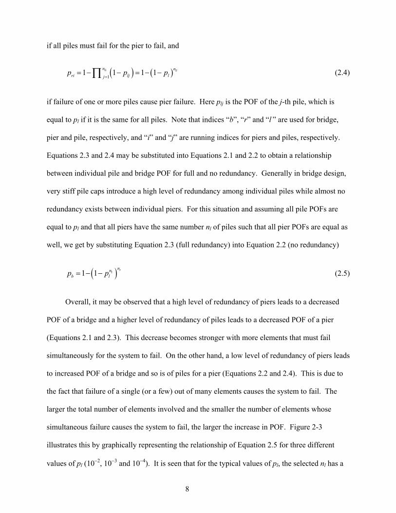
if all piles must fail for the pier to fail, and

1

1 1 1 1li lin n

ri lj ljp p p

(2.4)

if failure of one or more piles cause pier failure. Here plj is the POF of the j-th pile, which is

equal to pl if it is the same for all piles. Note that indices “b”, “r” and “l ” are used for bridge,

pier and pile, respectively, and “i” and “j” are running indices for piers and piles, respectively.

Equations 2.3 and 2.4 may be substituted into Equations 2.1 and 2.2 to obtain a relationship

between individual pile and bridge POF for full and no redundancy. Generally in bridge design,

very stiff pile caps introduce a high level of redundancy among individual piles while almost no

redundancy exists between individual piers. For this situation and assuming all pile POFs are

equal to pl and that all piers have the same number nl of piles such that all pier POFs are equal as

well, we get by substituting Equation 2.3 (full redundancy) into Equation 2.2 (no redundancy)

1 1rnn

b lp p l (2.5)

Overall, it may be observed that a high level of redundancy of piers leads to a decreased

POF of a bridge and a higher level of redundancy of piles leads to a decreased POF of a pier

(Equations 2.1 and 2.3). This decrease becomes stronger with more elements that must fail

simultaneously for the system to fail. On the other hand, a low level of redundancy of piers leads

to increased POF of a bridge and so is of piles for a pier (Equations 2.2 and 2.4). This is due to

the fact that failure of a single (or a few) out of many elements causes the system to fail. The

larger the total number of elements involved and the smaller the number of elements whose

simultaneous failure causes the system to fail, the larger the increase in POF. Figure 2-3

illustrates this by graphically representing the relationship of Equation 2.5 for three different

values of pl (102, 103 and 104). It is seen that for the typical values of pl, the selected nl has a

9

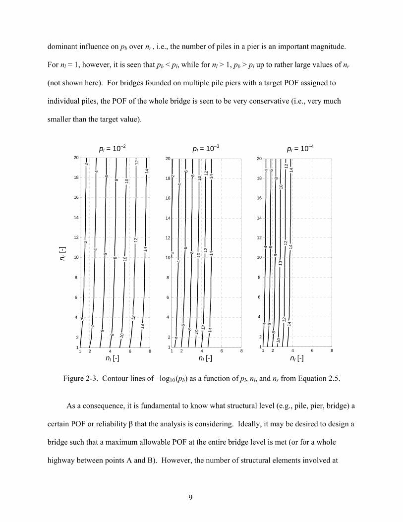
dominant influence on pb over nr , i.e., the number of piles in a pier is an important magnitude.

For nl = 1, however, it is seen that pb < pl, while for nl > 1, pb > pl up to rather large values of nr

(not shown here). For bridges founded on multiple pile piers with a target POF assigned to

individual piles, the POF of the whole bridge is seen to be very conservative (i.e., very much

smaller than the target value).

22

2

44

4

66

6

88

8

1010

10

1212

1214

1414

nl [-]

n r [-]

pl = 10-2

1 2 4 6 81

2

4

6

8

10

12

14

16

18

20

22

44

4

66

6

88

8

1010

10

1212

1214

1414

nl [-]

pl = 10-3

1 2 4 6 81

2

4

6

8

10

12

14

16

18

20

44

4

66

6

88

8

1010

1012

1212

1414

14

nl [-]

pl = 10-4

1 2 4 6 81

2

4

6

8

10

12

14

16

18

20

Figure 2-3. Contour lines of –log10(pb) as a function of pl, nl, and nr from Equation 2.5.

As a consequence, it is fundamental to know what structural level (e.g., pile, pier, bridge) a

certain POF or reliability β that the analysis is considering. Ideally, it may be desired to design a

bridge such that a maximum allowable POF at the entire bridge level is met (or for a whole

highway between points A and B). However, the number of structural elements involved at

pl = 102 pl = 103 pl = 104

nl [-] nl [-] nl [-]

n r [-

]

10

bridge level is quite large and generally outside the geotechnical field. Based on the latter and

the fact that design loads are typically given at the bridge pier level (rather than bridge level), it

is understood in what follows that values of POF β and, hence Φ, always correspond to the pier

level (i.e., for entire pile groups).

11

CHAPTER 3 SPATIAL UNCERTAINTY OF FB-DEEP SPT/CPT

CAPACITY ASSESSMENT

3.1 Background

For different combinations of soil conditions (e.g., sand, clay, etc.) and the type of

borehole data available (e.g., SPT or CPT), FB-Deep uses a series of simple relationships to

estimate total resistances of driven piles. Since it is assumed that a pile is driven at a particular

boring location (data along center line of pile), values of Φ only consider the uncertainty of the

estimation method. However, a pile may be driven at a random location at a site (i.e., without

collocated data) over which several SPT/CPT soundings may have been obtained. Quantifi-

cation of Φ in this case requires accounting for spatial variability, the effect of which is

investigated in the present chapter. For this purpose, the effect of method uncertainty is

neglected, however, it may be added back in without loss of applicability. For simplicity, a

single geological layer is assumed, which allows for deriving closed form solutions and

facilitating some insight into spatial upscaling of side friction and end bearing separately, as well

as in combination (side-tip correlation). Note, however, that the results are only applicable to the

FB-Deep methods identified.

3.2 Theory

Figure 3-1 shows a schematic of a driven pile of length L and diameter D along the center

line of which SPT or CPT data are available. Following the linear model implemented in

FB-Deep, mean unit side friction fs is estimated by

Ln

ii

Ls dzzN

L

SSN

nf

L

01

)(1

(3.1)

12

where Ni is the number of blow-counts per depth interval for SPT or the mean driving force over

a depth interval for CPT. The term nL represents the number of depth intervals over the pile

length L and S is a constant conversion factor from SPT or CPT data to unit side friction.

Figure 3-1. Schematic of driven pile (circular or square) with SPT or CPT data available along center line (dashed) for use in FB-Deep method.

Without loss of generality, depth intervals may be considered arbitrarily short leading to

the integral form of Equation 3.1 (i.e., line averaging) on the far right-hand-side, where z is the

vertical coordinate as indicated in Figure 3-1. From this, predicted pile side friction resistance Rs

results as

0

( )L

s sR DL f DS N z dz (3.2)

For predicting unit tip resistance qt (in a single layer), a linear FB-Deep model uses

DL

L

L

DL

n

jj

D

n

ii

Dt dzzN

D

TdzzN

D

TTN

nTN

nq

DD 5.3

815.318

)(5.3

)(82

111

2

1 5.38

(3.3)

D

L

8D

3.5D

z

13

where n8D and n3.5D are the number of depth intervals over distances 8D and 3.5D immediately

above and below the center of the pile tip as illustrated in Figure 3-1. Term T is a constant

conversion factor between SPT or CPT data and unit tip resistance. Predicted tip resistance Rt

results as

DL

L

L

DL

tt dzzNdzzN

DTqDR

5.3

8

2

)(5.3

8)(

644

(3.4)

Summing Equations 3.2 and 3.4 leads to the total pile resistance R as

3.5

0 8

8( ) ( ) ( )

64 3.5

L L L D

L D L

TR D S N z dz N z dz N z dz

(3.5)

which is a weighted integral of N over 0 ≤ z ≤ (L + 3.5D) and can be written equivalently as

DL

dzzNzgDR5.3

0

)()( (3.6)

where

D.LzLT

LzDLT

S

DLzS

zg

53for 28

8for 64

80for

)( (3.7)

Regarding N as a spatially random function in a geostatistical sense with mean μN, variance

2N and spatial covariance function CN, then the mean μR and variance 2

R of total pile resistance,

R may be found. Taking the mean (expectation) of Equation 3.6 gives

14

NNN

DL

NR TD

SDLTD

SLDdzzgD 44

)(25.3

0

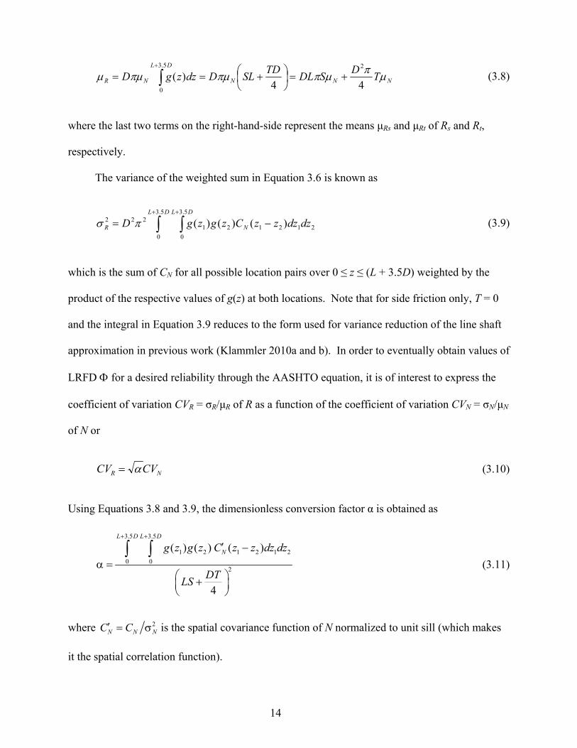
(3.8)

where the last two terms on the right-hand-side represent the means μRs and μRt of Rs and Rt,

respectively.

The variance of the weighted sum in Equation 3.6 is known as

2

5.3

0

5.3

0

12121222 )()()( dzdzzzCzgzgD

DL DL

NR

(3.9)

which is the sum of CN for all possible location pairs over 0 ≤ z ≤ (L + 3.5D) weighted by the

product of the respective values of g(z) at both locations. Note that for side friction only, T = 0

and the integral in Equation 3.9 reduces to the form used for variance reduction of the line shaft

approximation in previous work (Klammler 2010a and b). In order to eventually obtain values of

LRFD for a desired reliability through the AASHTO equation, it is of interest to express the

coefficient of variation CVR = σR/μR of R as a function of the coefficient of variation CVN = σN/μN

of N or

NR CVCV (3.10)

Using Equations 3.8 and 3.9, the dimensionless conversion factor α is obtained as

3.5 3.5

1 2 1 2 1 2

0 02

( ) ( ) ( )

4

L D L D

Ng z g z C z z dz dz

DTLS

(3.11)

where 2N N NC C is the spatial covariance function of N normalized to unit sill (which makes

it the spatial correlation function).

15

Combining Equations 3.7 and 3.11 α may be written as

6543212

2224

16IIIIII

DTLS

(3.12)

which is proportional to the sum of the following six integrals:

2

8

5.3

121

2

6

2

0

5.3

1215

2

0 8

1214

2

5.3 5.3

1212

2

3

2

8 8

1212

2

2

2

0 0

1212

1

)('6428

)('28

)('64

)('28

)('64

)('

dzdzzzCT

I

dzdzzzCST

I

dzdzzzCST

I

dzdzzzCT

I

dzdzzzCT

I

dzdzzzCSI

L

DL

DL

L

N

L DL

L

N

L L

dL

N

DL

L

DL

L

N

L

DL

L

DL

N

L L

N

(3.13)

Using Equation 3.13 with Equation 3.9, it may be seen that I1 and I2 correspond to the respective

variances of the side and tip resistance along the pile; I3 corresponds to the average below the tip;

and I4, I5, and I6 correspond to the respective covariances. As mentioned above, for side friction

only T=0 and only I1 remains non-zero. Furthermore, the sum I2 + I3 + 2I6 corresponds to the

variance of Rt while the sum I4 + I5 corresponds to the covariance between Rs and Rt. Thus, by

splitting up the integral in Equation 3.9 (e.g., as done in Equation 3.13) different variance and

covariance components may be isolated. For example, I4 = I41 + I42 may be written with

41 1 2 1 2

8 8

8

42 1 2 1 2

0 8

( )64

( )64

L L

N

L D L D

L D L

N

L D

STI C z z dz dz

STI C z z dz dz

(3.14)

16

With this, the integrals in I1, I2, I3, and I41 are of the form 1 2 1 2( )b b

N

a a

A C z z dz dz , while I42, I5

and I6 are of the form 1 2 1 2( )b c

N

a b

B C z z dz dz , where a, b and c are variable integration limits.

Assuming that CN is of the spherical type

31 1.5 0.5 for 1( )

0 for 1N

h h hC h

h

(3.15)

where h = |z1 – z2|/av and av is the vertical correlation length of N, the integral of type A has been

solved in Appendix B of Final Project Report BD-545-76. Although mathematically simple, use

of Equation 3.15 in the sequel requires lengthy algebraic manipulations and numerous case

distinctions due to the separate definition of CN on the intervals h < 1 and h < 1. Therefore, the

exponential covariance function

3( ) hNC h e (3.16)

is used in the analytical development hereafter. For direct numerical integration of Equation

3.11, however, both Equations 3.15 and 3.16 will be evaluated. As shown in Final Project

Report BD-545-76 (Figures 3-1 and 3-2) in a closely related context, differences between

Equations 3.15 and 3.16 when used with same av are negligible for all practical purposes.

Moreover, the decision whether Equation 3.15 or 3.16 (or some other covariance model) is most

adequate is mostly based on limited data (experimental variogram) and, hence, rather arbitrary or

subjective.

Integral A will be solved here using Lab = |a – b|/av by transforming the double integral in

dz1 and dz2 into a single integral in dh giving

0

2 ( )abL

ab NA L h C h dh (3.17)

17

That is, instead of effectively pairing up all possible locations z1 and z2 over Lab in the double

integral, Equation 3.17 uses the frequency of occurrence of each separation distance h between

all possible location pairs on Lab (see Figure 3-2) which is equal to 2(Lab – h) as apparent in the

integrand of Equation 3.17. Combining Equations 3.16 and 3.17 and knowing that

12

kxk

edxxe

kxkx gives

abL

ab

ab eL

LA 31

3

11

3

2 (3.18)

This result may be validated against results of numerical integration shown in Figure 3-2 (for

D/ah = 0) of Final Project Report BD-545-76 (note that their = 2abA L here).

Figure 3-2. Illustration of how the double integral in A may be converted into a single integral using the frequency of occurrence of location pairs

on Lab, which are separated by distance h.

Integral B may be solved using Lab as above and Lbc = |b – c|/av, where Lbc ≤ Lab is assumed

without loss of generality (the order of integration in all double integrals above may be switched

without affecting the results). The double integral in dz1 and dz2 may be transformed into a

single integral in dh giving

0

'( ) ( ) ( )bc ab ab bc

bc ab

L L L L

N bc N ab bc N

L L

B hC h dh L C h dh L L h C h dh

(3.19)

a b

Lab

h

18

Instead of effectively pairing up all possible location z1 and z2 in the double integral, Equation

3.19 uses the frequency of occurrence of each separation distance h between all possible location

pairs of one point on Lab and the other point on Lbc. This is illustrated in Figure 3-3 and the

coefficients inside the integrands of Equation 3.19 indicate that separation distances between

zero and Lbc occur h times, between Lbc and Lab they occur Lbc times, and between Lab and

Lab+Lbc they occur Lab + Lbc – h times. Location pairs of h > Lab + Lbc cannot occur.

Figure 3-3. Illustration of how the double integral in B may be converted into a single integral using the frequency of occurrence of location pairs between

Lab and Lbc, which are separated by distance h.

Combining Equations 3.16 and 3.19 gives after some manipulations

33 311

9ab bcab bc L LL LB e e e (3.20)

which shows the convenient fact that the condition Lbc ≤ Lab established for building Equation

3.19 becomes irrelevant (Lab and Lbc may be switched in Equation 3.20 without affecting B).

Using Equations 3.18 and 3.20, the integrals of Equations 3.13 and 3.14 may be found

using L = L/av, D = D/av and the following equivalences: Lab = L in A for I1; Lab = 8D in A for

I2; Lab = 3.5D for A in I3; Lab = 8D in A for I41; Lab = L – 8D and Lbc = 8D in B for I42; Lab = L

and Lbc = 3.5D for B in I5; and Lab = 8D and Lbc = 3.5D in B for I6. Substituting the results into

Equation 3.12 gives

a b c

Lab Lbc

h ≤ Lbc

Lbc ≤ h ≤ Lab

Lab ≤ h ≤ Lab + Lbc

19

2 2

23 24

2

10.5 34.5

193 9 2 6 3 23 1

2048 49 32 7 2 128 7

9 2 9 1

32 7 2048 7 321

1 9 1 1 134

128 49 14 128 7 14

TS TS TS TS

L D

TS TS TS

LDD D

TSTS TS

L DR R R R

e eR R R

RD e e eR

R R

3 3.5

3 81

32

L D

L D

TS

eR

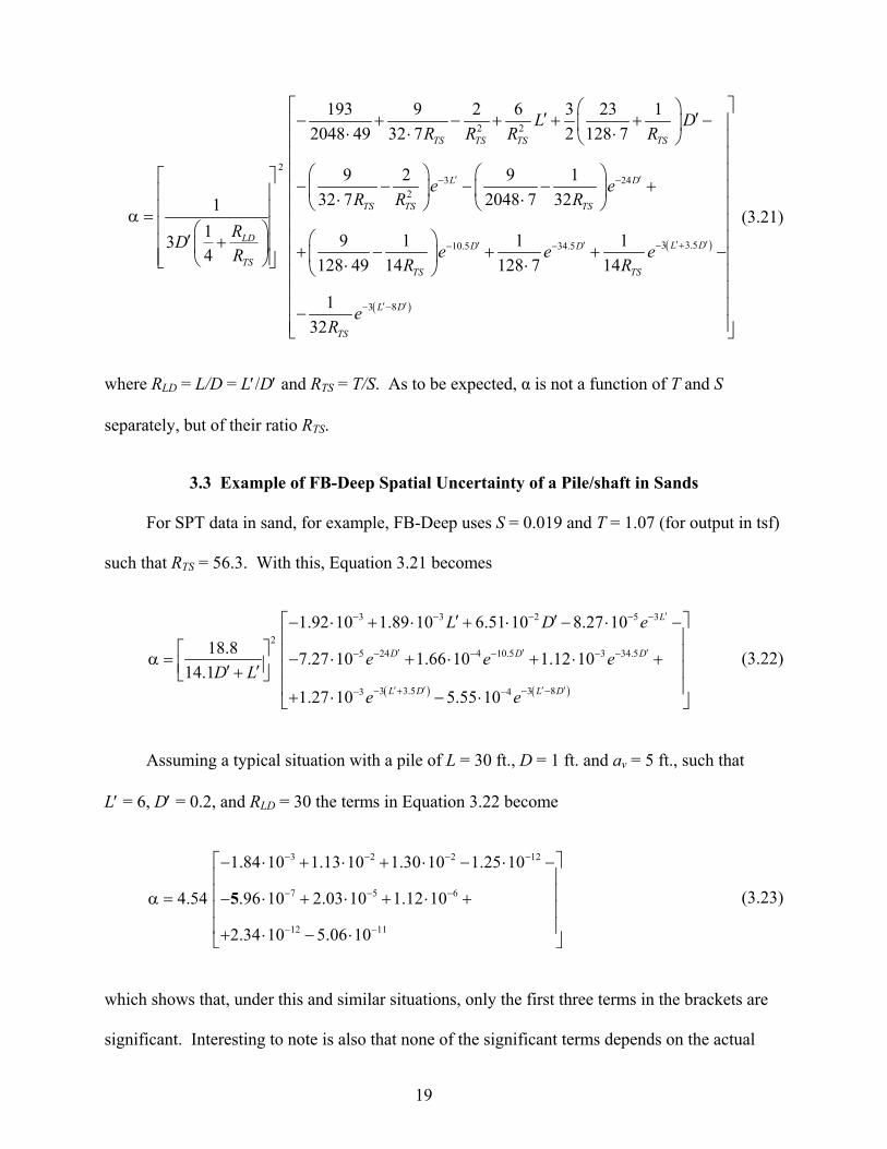
(3.21)

where RLD = L/D = L/D and RTS = T/S. As to be expected, α is not a function of T and S

separately, but of their ratio RTS.

3.3 Example of FB-Deep Spatial Uncertainty of a Pile/shaft in Sands

For SPT data in sand, for example, FB-Deep uses S = 0.019 and T = 1.07 (for output in tsf)

such that RTS = 56.3. With this, Equation 3.21 becomes

3 3 2 5 3

25 24 4 10.5 3 34.5

3 3.5 3 83 4

1.92 10 1.89 10 6.51 10 8.27 10

18.87.27 10 1.66 10 1.12 10

14.1

1.27 10 5.55 10

L

D D D

L D L D

L D e

e e eD L

e e

(3.22)

Assuming a typical situation with a pile of L = 30 ft., D = 1 ft. and av = 5 ft., such that

L=6, D = 0.2, and RLD = 30 the terms in Equation 3.22 become

3 2 2 12

7 5 6

12 11

1.84 10 1.13 10 1.30 10 1.25 10

4.54 .96 10 2.03 10 1.12 10

2.34 10 5.06 10

5 (3.23)

which shows that, under this and similar situations, only the first three terms in the brackets are

significant. Interesting to note is also that none of the significant terms depends on the actual

20

shape of the spatial covariance function (i.e., the exponential function in this case), but merely

contain L and D expressing how many times L and D contain av. With this an approximation of

Equation 3.22 may be written in a rational form as

2

0.668 23.0 0.679

14.1

L D

L D

(3.24)

Figures 3-4 and 3-5 graphically represent results of Equations 3.22 and 3.24 for L/D ≥ 8.

The dashed line in Figure 3-4 is from Equation 3.22, where T was previously set to zero in

Equation 3.21. Term T = 0 means that end bearing is excluded from consideration and the

problem is based on side friction along a vertical line only (“line shaft approximation”). The

dashed line appears to act as an upper bound for the continuous lines of T > 0, however, this is

not generally true for other values of S and T. The approximations in Figure 3-5 are seen to be

valid for L/av > 1.5, which is reasonable for practice. Figures 3-6 and 3-7 are analogous to

Figures 3-4 and 3-5, with the exception that a spherical covariance model (Equation 3.15) is used

instead of an exponential covariance model (Equation 3.16) and that graphs are obtained from

numerical integration of Equation 3.11. In order for Equation 3.24 to be also a good approxi-

mation for the spherical covariance model, 1/2 from Equation 3.24 must be multiplied by 1.07.

Note also that Figures 3-4 through 3-7 may be directly plugged into quadrant charts developed in

previous work (Final Project Report BD-545-76) which allows for direct determination of

required pile length L for given D, μN, CVN, reliability and design load Qdes. The correspon-

ding design situation would be of possessing exhaustive sample data of N over a site associated

with a random pile location.

21

0 2 4 6 8 10 12 14 16 18 200.1

0.2

0.3

0.4

0.5

0.6

0.7

0.8

0.9

1

L/av [-]

1/

2 [-]

EXPONENTIAL

Figure 3-4. 1/2 from Equation 3.22 for exponential covariance function (Equation 3.16).

Continuous lines from bottom up are for L/D = {8, 10, 15, ≥ 30}. Dashed line is for T = 0, i.e., side friction only (“line shaft approximation”).

0 2 4 6 8 10 12 14 16 18 200

0.1

0.2

0.3

0.4

0.5

0.6

0.7

0.8

0.9

1

L/av [-]

1

/2 [-

]

EXPONENTIAL

Figure 3-5. 1/2 from Equation 3.22 (continuous) and its rational approximation from Equation 3.24 (dashed) valid for L/av > 1.5. Lines from

bottom up are for L/D = {8, 10, 15, ≥ 30}.

22

0 2 4 6 8 10 12 14 16 18 200

0.1

0.2

0.3

0.4

0.5

0.6

0.7

0.8

0.9

1

L/av [-]

1

/2 [-

]

SPHERICAL

Figure 3-6. 1/2 from numerical integration of Equation 3.11 for spherical covariance function (Equation 3.15). Continuous lines from bottom up are for L/D = {8, 10, 15, ≥ 30}.

Dashed line is for T = 0, i.e., side friction only (“line shaft approximation”).

0 2 4 6 8 10 12 14 16 18 200

0.1

0.2

0.3

0.4

0.5

0.6

0.7

0.8

0.9

1

L/av [-]

1

/2 [-

]

SPHERICAL

Figure 3-7. 1/2 from numerical integration of Equation 3.11 (continuous) and a rational approximation as 1.07 times from Equation 3.24 (dashed). Approximation valid

for L/av > 1.5 with L/D ≥ 15 and for L/av > 3 with L/D > 15. Lines from bottom up are for L/D = {8, 10, 15, ≥ 30}.

23

CHAPTER 4 PILE GROUP SPATIAL UNCERTAINTY

WITH NEARBY SPT/CPT DATA

4.1 Background

The previous chapter considers exhaustive borehole (i.e., SPT or CPT) data available at a

site where the influence of spatial variability on total pile resistance is investigated. The pile was

considered to be randomly located or, equivalently, located beyond the spatial correlation range

from available data. The present chapter expands on this by assuming SPT/CPT data from a

limited number of borings, where spatial correlation between a “nearby” boring and the

foundation may be present. Moreover, the analysis is generalized to allow for one or more piles

in a group with tip resistance neglected until the next chapter for simplicity. As such, results are

equally applicable to single or groups of drilled shafts with local strength data available from a

number of borings which is the scenario providing the terminology used in the remainder of this

chapter. A detailed discussion and analysis of worst case scenarios for unknown horizontal

correlation lengths is illustrated by an example calculation at the conclusion of the chapter.

4.2 Notation

The term q(x) denotes a spatially variable (random) function for local ground (i.e., soil or

rock) strength with x being a spatial coordinate vector. The term q(x) — or in short q — is

described by a mean μq, variance 2q and a spatial covariance function Cq(h) — or in short Cq —

with h being a spatial separation vector between two locations x1 and x2. Variable Cq may be

anisotropic with a range ah in all horizontal directions and a range av in the vertical direction. A

normalized spatial covariance function qC (hi) = Cq(hi)/2q of unit sill and unit isotropic range

may be defined by using 22vvhhi ahahh where hh and hv are the horizontal and vertical

24

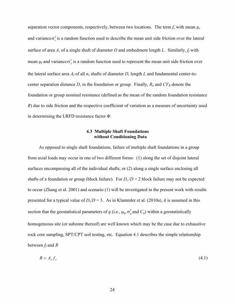
separation vector components, respectively, between two locations. The term fs with mean μs

and variance 2s is a random function used to describe the mean unit side friction over the lateral

surface of area As of a single shaft of diameter D and embedment length L. Similarly, ff with

mean μf and variance 2f is a random function used to represent the mean unit side friction over

the lateral surface area Af of all ns shafts of diameter D, length L and fundamental center-to-

center separation distance Ds in the foundation or group. Finally, Rn and CVR denote the

foundation or group nominal resistance (defined as the mean of the random foundation resistance

R) due to side friction and the respective coefficient of variation as a measure of uncertainty used

in determining the LRFD resistance factor Φ.

4.3 Multiple Shaft Foundations without Conditioning Data

As opposed to single shaft foundations, failure of multiple shaft foundations in a group

from axial loads may occur in one of two different forms: (1) along the set of disjoint lateral

surfaces encompassing all of the individual shafts; or (2) along a single surface enclosing all

shafts of a foundation or group (block failure). For Ds /D > 2 block failure may not be expected

to occur (Zhang et al. 2001) and scenario (1) will be investigated in the present work with results

presented for a typical value of Ds/D = 3. As in Klammler et al. (2010a), it is assumed in this

section that the geostatistical parameters of q (i.e., μq,2q and Cq) within a geostatistically

homogeneous site (or subzone thereof) are well known which may be the case due to exhaustive

rock core sampling, SPT/CPT soil testing, etc. Equation 4.1 describes the simple relationship

between ff and R

ff fAR (4.1)

25

where Af = ns LDπ is considered deterministic, i.e., with negligible uncertainty compared to ff.

Rand ff are random variables linked to q by the spatial upscaling (arithmetic averaging) process

1

f

ff A

f q dAA

(4.2)

By taking the expectation and variance of Equation 4.2, the parameters μf and 2f are found as

(Journel and Huijbregts 1978)

qf (4.3)

22

1 22

f f

qf q

f A A

C dA dAA

(4.4)

where a variance reduction factor αqf between local strength q and mean foundation unit side

friction ff may be defined as

qssfq

ssf

q

fqf

2

2

2

2

(4.5)

which links the variability in local strength q to the uncertainty in foundation or group resistance

R by CVR = 1/ 2qf CVq (“CV” being the notation for coefficient of variation of the variable in the

index). Term αsf in Equation 4.5 denotes an intermediate variance reduction factor between

single shaft unit side friction fs and the foundation unit side friction ff. Furthermore, αqs

quantifies the variance reduction between local strength q and fs as studied by Klammler et al.

(2010a). The double integral in Equation 4.4 is nothing but the summation of the normalized

covariance values between all possible combinations of point pairs on the ns lateral shaft surfaces

(i.e., the sum of all elements in the variance–covariance matrix between all possible point pairs)

and may be evaluated numerically by discretizing each shaft surface into a large enough number

of points (Journel and Huijbregts 1978). Calculations may hereby be accelerated by recognizing

26

that center-to-center separation distances between different shaft pairs are limited to a certain

pattern (e.g., 3D for all shaft pairs on a side of a quadruple square foundation and 3 2D for

shaft pairs on a diagonal). Thus, normalized covariances sC (hs) = 2( )s s sC h between upscaled

single shaft resistances fs (with hs representing the horizontal separation distance between shaft

centers) may be determined for these separation distances by using Equation 4.6 (Journel and

Huijbregts 1978) to populate a respective variance–covariance matrix between all individual

shafts in a foundation through

1 2

2

1 221 2

( )s s

qs s q

s s s A A

C h C dA dAA A

(4.6)

where As1 and As2 are the lateral surface areas of two horizontally offset shafts. Equation 4.6 is,

in fact, a generalization of Equation 4.4 (normalized to 2 ,s i.e., unit sill) which is obtained by

setting As1 = As2 = Af , i.e., the total of all shafts’ lateral surfaces. For As1 = As2 = LDπ, i.e., a

single shaft’s lateral surface or zero separation between two shafts, Equation 4.6 reduces to the

upscaled variance of fs for single shafts as in Klammler et al. (2010a).

Figure 4-1 shows an example of a quadruple square configuration (hereafter called “Q”)

with respective shaft separation and variance–covariance matrices. The matrix in Figure 4-1c is

based on numerical integration of Equation 4.6 where a spherical covariance function Cq is used

with parameters L/av = 5 and D/ah = 0.1. Based on the same principle of Equation 4.6, the

average of all the elements in the variance–covariance matrix of all shafts directly results in the

respective variance reduction factor sf defined in Equation 4.5. The shape of sC from Equation

4.6 is not easily described analytically; however, its horizontal correlation range is known to be

equal to ah + D corresponding to the minimum horizontal separation distance between shaft

centers for which all location pairs between shafts are beyond ah and, thus, uncorrelated. Based

27

on this, an approximation to ,sC i.e., Equation 4.7, is proposed in the form of a spherical

covariance function of range ah + D, which avoids the numerical integration of Equation 4.6 and

allows for a quick and direct population of the respective shaft variance–covariance matrix as

shown in Figure 4-1d.

3

1 1.5 0.5 for 1

( )

0 for 1

s s s

h h h

s s

s

h

h h h

a D a D a DC h

h

a D

(4.7)

Figure 4-1. (a) Example of quadruple “Q” square configuration with (b) respective shaft separa-

tion matrix in multiples of D, and (c) and (d) are variance–covariance matrices in multiples of the upscaled single shaft variance 2.s Part (c) is from numerical evaluation of Equation 4.6,

while Part (d) assumes a spherical covariance function of range ah + D to approximate the horizontal covariance function Cs (Equation 4.7). A spherical covariance function for

q and L/av = 5 and ah/D = 10 are used. Bold italic numbers indicate shaft numeration and are used to label rows and columns of the matrices.

(b) 1 2 3 4

1 0 3 4.2 3

2 3 0 3 4.2

3 4.2 3 0 3

4 3 4.2 3 0

(c) 1 2 3 4 (d) 1 2 3 4

1 1 0.68 0.48 0.68 1 1 0.60 0.45 0.60

2 0.68 1 0.68 0.48 2 0.60 1 0.60 0.45

3 0.48 0.68 1 0.68 3 0.45 0.60 1 0.60

4 0.68 0.48 0.68 1 4 0.60 0.45 0.60 1

1

2 3

4

(a)

D

D

28

In addition to the quadruple configuration of Figure 4-1a, Figure 4-2 illustrates further

multiple shaft configurations considered in this work (D1, T1 and T2). In analogy to Figure 4-1,

for every configuration considered here and associated shaft separation distances, the variance–

covariance matrices may be constructed using Equation 4.6 or 4.7 and αsf may be found by

averaging of all matrix elements. The averaging of the matrix elements may be summarized by

the following equations where the type of foundation is indicated in the subscripts. Extensions to

other group configurations not considered herein are straightforward.

,

, 1

, 2

,

0.5 (0) 0.5 ( )

0.33(0) 0.44 ( ) 0.22 (2 )

0.33 (0) 0.67 ( )

0.25 (0) 0.5 ( ) 0.25 ( 2 )

sf D s s s

sf T s s s s

sf T s s s

sf Q s s s s s

C C D

C D C D

C C D

C C D C D

(4.8)

Figure 4-2. Further examples of multiple shaft configurations with rigid pile caps and possible center borings (crosses).

For the exact solution of Equation 4.6, values of sC and αsf in Equation 4.8 are a function of

L/av, D/ah and Ds /D. For a typical value of Ds /D = 3 and using Equations 4.5 and 4.8, Figure

4-3 graphically represents the outcome of the exact solution of 1/ 2qf for different shaft

configurations (single shafts “S ” from Klammler et al. 2010b is included for reference). Using

the approximation of Equation 4.7 (not shown for clearness of charts) instead of Equation 4.6

D

Ds Ds

D1

T

T

29

results in maximum errors in 1/ 2qf (and hence CVR for a given CVq) of approximately ±5 %.

Errors are close to zero for D/ah < 0.05, D/ah ≈ 0.15 and D/ah > 0.5. For 0.05 < D/ah < 0.15

errors are negative (i.e., unconservative, which may be avoided by multiplication of 1/ 2qf by 1.05

in this range), while for 0.15 < D/ah < 0.5 errors are positive. Maximum positive and negative

errors of the approximation also decrease as Ds /D increases and unconservative errors do not

exceed 5% down to a theoretical value of Ds /D = 1 (results not shown).

Figure 4-3. 1/ 2qf as a function of L/av for single and multiple shaft configurations of Figures 4-1

and 4-2 with Ds /D = 3. Thick graph corresponds to line shaft approximation 1/ 20 .

The top graphs (case of D/ah = 0) in Figure 4-3 are all identical; in this case the variance

reduction is independent of the number and arrangement of shafts and equal to variance

reduction α0 for averaging over a vertical line of length L (termed “line shaft approximation” in

Klammler et al. 2010a and b)

T2

D1 T1S

Q

30

3

0 3

2

0 2

1 for 0 12 20

3 for 1

4 5

v v v

v v

v

L L L

a a a

a a L

L L a

(4.9)

This is seen to be the common worst case scenario (maximum αqf and CVR) for all configurations

in the case of potentially unknown ah. For D/ah > 0.5 correlation between individual shafts is

zero and sf from shaft to foundation level becomes equal to 1/ns. Based on the assumption of

lognormality for foundation resistance and computed CVR, determination of LRFD resistance

factor Φ may be achieved along the lines of Klammler et al. (2010a) by the following AASHTO

(2004) formulae:

2

2

2 2

1

1

exp ln 1 1

QDR D L

L R

DQD QL R Q

L

CVQQ CV

QCV CV

Q

(4.10)

2

2

2

2

2

2 QLQLQDL

DQD

L

D

QLQLQDQDL

D

Q

Q

Q

Q

Q

CVCVQ

Q

CV

(4.11)

The term CVQ hereby denotes the coefficient of variation of the random load and β is a

user selected reliability index depending on the importance of a structure (admissible probability

of failure). The remaining dimensionless parameters in Equations 4.10 and 4.11 may be chosen

according to AASHTO (2004) for load cases I, II, and IV where dead load factor γD = 1.25, live

load factor γL = 1.75, and the Federal Highway Administration (FHWA) recommended values of

dead-to-live load ratio QD /QL = 2, resistance bias factor λR = 1.06, dead load bias factor λQD =

1.08, live load bias factor λQL = 1.15, dead load coefficient of variation CVQD = 0.128 and live

load coefficient of variation CVQL = 0.18. It is worthwhile noting that Φ from Equation 4.10 is

31

based on CVR of the whole foundation and, as such, assures a target probability of failure of the

whole foundation and not just of a single shaft of the group (which would not be the actual

design goal).

4.4 Single and Multiple Shaft Foundations with Conditioning Data

Knowing the exact locations of each foundation in the design process allows for collection

of additional boring data inside or near the footprint (e.g., at the center as indicated by crosses in

Figures 4-1 and 4-2 and considered hereafter) of a foundation to decrease uncertainty in

predicted foundation resistances. In order to incorporate the influence of such collocated boring

data, spatial correlation (conditioning) between data and the foundation is explored. The

geostatistical tool used for this purpose is ordinary kriging (Journel and Huijbregts 1978), which

delivers a predicted mean unit side friction ff with an error variance 2fk between ff and its true

counterpart ff . The resulting problem may be studied in a two-dimensional (horizontal) plane

where each of nb borings on a site is represented by a point associated to a data value equal to the

mean qbi (i = 1, 2… nb) of the local strength observations in that boring (assuming that all

borings are of approximately same length L). The foundation is represented by its horizontal

cross section centered on one of the borings as illustrated by Figure 4-4.

Figure 4-4. Typical plan view of borehole (crosses) and foundation locations (e.g., quadruple shaft foundation for a bridge site). Not to scale.

For a full ordinary kriging solution, the horizontal covariances among all the borings

themselves and between all the borings and the foundation would be required in order to

32

determine a specific kriging weight wi (Σwi = 1) for each boring. The term ff as given by

Equation 4.2 is then predicted in the well known form by

1

bn

f i bii

f w q

(4.12)

with a variance 2fk of the prediction error ff – ff as

bb b n

ifibfi

n

i

n

jjibjiffk xxCwxxCww

11 1

22 )(2)( (4.13)

where Cb is the horizontal covariance function of qb (i.e., a vertically upscaled version of Cq

according to Equation 4.6) between boring locations xi and xj, and Cbf is the horizontal

covariance function between qb and ff with xf denoting the (center) location of the foundation. It

is hereby assumed that the borings are sampled at intervals smaller than av such that additional

sampling in a boring would only deliver highly redundant (i.e., correlated) information. With

this, each boring may be considered as continuously sampled over depth and the actual numbers

of samples per boring become irrelevant (i.e., do not appear in Equations 4.12 and 4.13). The

three terms on the right-hand-side of Equation 4.13 are the variance 2f of ff (Equation 4.4), the

variance 2f of ff and twice the covariance ( , )f fC f f between ff and ff whose negative sign

reflects the benefit of conditioning data on prediction uncertainty. All terms may be directly

obtained from Equation 4.6 with respective choices of A1 and A2.

In typical design situations, nb borings at a site may consist of n1 largely spaced borings

from preliminary site investigation (i.e., previous to definition of foundation locations) and n2

subsequent borings at potential foundation locations. In such cases, it may be reasonable to

assume that no correlation exists between the borings at a site (i.e., Cb(xi-xj) = Cb(0) for i = j and

equal to zero otherwise), except for when a preliminary boring happens to be in the vicinity of a

future foundation location where a collocated boring is also obtained. In such a case, it is

33

conservative to consider full correlation between such nearby pairs of borings and reduce them to

one “effective” boring by averaging (a non-simplified ordinary kriging solution would do the

same). Thus, a conservative “effective” number of uncorrelated borings is obtained as nbe ≤ nb

(e.g., in Figure 4-4 nb = 8 and nbe = 6). With the further assumption that only the collocated

boring (i = 1) presents possible spatial correlation with ff (i.e., Cbf (xi-xf) = Cbf (x1-xf) for i = 1 and

zero otherwise, a very simple ordinary kriging system may be constructed for determination of

the kriging weights wi as represented by Equation 4.14. The term w1 represents the weight for

the collocated boring, w2 = (1 – w1)/(nbe – 1) the equal weights for all other borings (wi = w2 for

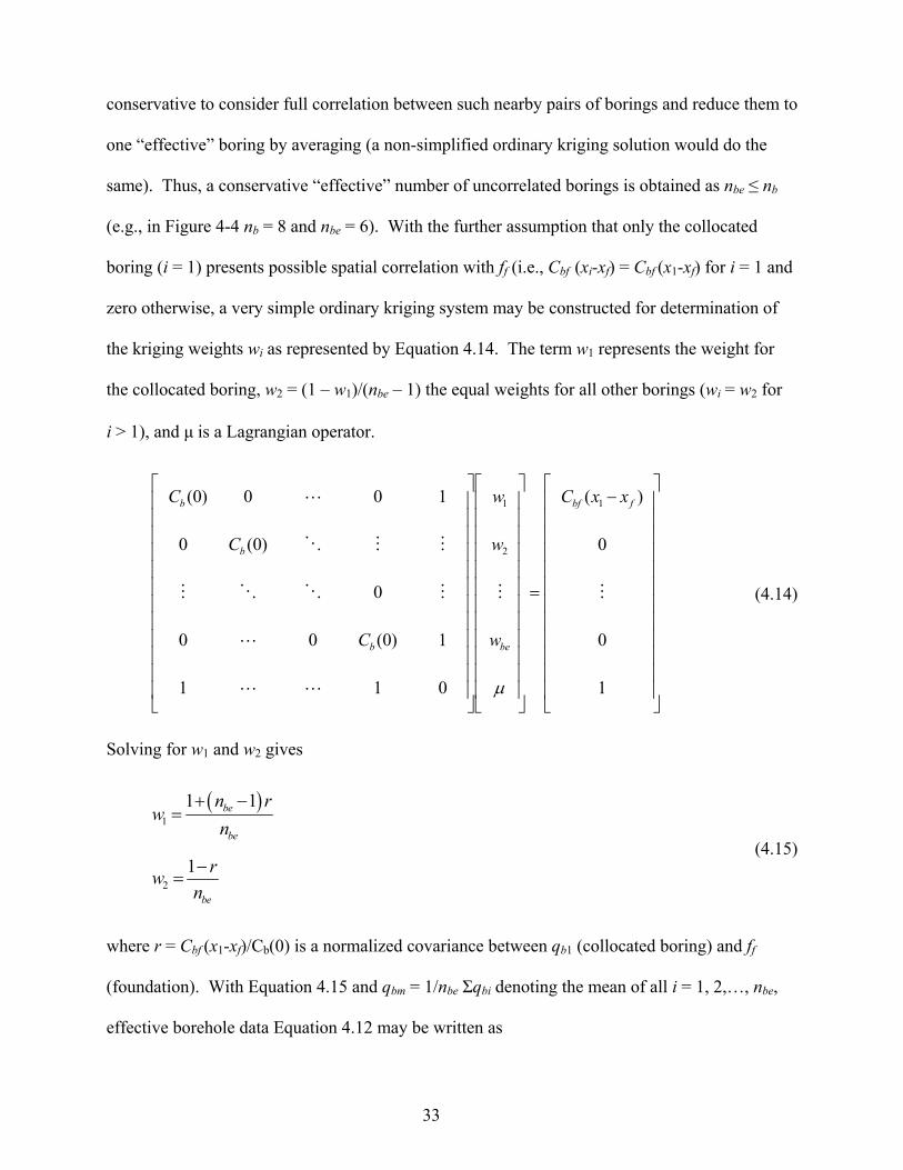
i>1), and μ is a Lagrangian operator.

1

0

0

)(

011

1)0(00

0

)0(0

100)0( 1

2

1

fbf

beb

b

b xxC

w

w

w

C

C

C

(4.14)

Solving for w1 and w2 gives

1

2

1 1

1

be

be

be

n rw

n

rw

n

(4.15)

where r = Cbf (x1-xf)/Cb(0) is a normalized covariance between qb1 (collocated boring) and ff

(foundation). With Equation 4.15 and qbm = 1/nbe Σqbi denoting the mean of all i = 1, 2,…, nbe,

effective borehole data Equation 4.12 may be written as

34

1 1f b bmf rq r q (4.16)

For r = 0, the collocated boring has no more predictive power than the other borings

and ff =qbm, while for r = 1 the collocated boring is a perfect predictor such that ff = qb1.

Substituting Equation 4.15 into Equation 4.13 under the above assumptions about Cb and Cbf,

simplifying and dividing by 2q gives

qf

beq

fkqfk r

n

r

2

2

02

21

(4.17)

as a respective variance reduction factor which accounts for limited data through nbe and data

conditioning through r. Theoretically perfect prediction with r = 1 is possible only if the

foundation is reduced to a vertical line (identical to the collocated boring), such that αqf = α0

correctly leading to αqfk = 0. For the opposite case of r = 0 (no conditioning to nearby data or

random/unknown foundation location) and the conservative line shaft approximation (αqf = α0)

Equation 4.17 reduces to a respective expression developed in Klammler et al. (2010b) for the

presence of a limited number of test borings. Finally, Equation 4.17 is seen to correctly reduce

to αqfk = αqf of the previous section for r = 0 and nbe >> 1, i.e., no data conditioning and

exhaustive data set available.

Equations 4.16 and 4.17 are directly valid for any type of single or multiple shaft

foundation and required values of α0 and αqf may be readily obtained from Figure 4-3 and/or

Equation 4.9. What remains to be determined is the correlation parameter r, which is obtained

from Equation 4.6 with A1 being a vertical line of length L (collocated boring) and A2 being the

total lateral foundation surface Af. As such, Equations 4.16 and 4.17 are generally valid for

arbitrary boring locations inside or nearby the foundation footprint. For the particular (but quite

35

typical) case of a boring at the center of the footprint (i.e., x1 = xf), results from numerical

integration of Equation 4.6 are graphically represented in Figure 4-5 as a function of ah /D for

various shaft configurations. As to be expected, spatial correlation in the vertical direction only

has a small influence on the horizontal correlation parameter r with this influence becoming

quite insignificant for L/av > 1. The latter is also the range encountered in practical applications

for which Figure 4-5 is valid (L/av < 1 would be reflected by a non-stationary variogram over the

foundation depths and would be handled by subtraction of a deterministic trend function such

that L/av > 1 is again the case for the random residuals).

0 2 4 6 8 10 12 14 16 18 200

0.1

0.2

0.3

0.4

0.5

0.6

0.7

0.8

0.9

1

ah/D [-]

r [-

]

Q

T2

D

T1

S

Figure 4-5. The term r = Cbf (0)/Cb(0) as a function of ah /D for L/av > 1 (continuous), L/av = 0 (dashed) and different shaft configurations (Ds = 3D).

For given foundation types (S, D1, T1, T2 or Q), dimensions (D and L; Ds = 3D) and site

conditions (qb1, qbm, CVq, av and ah) Figure 4-5 with Equations 4.16 and 4.17 can be used to find

a nominal resistance Rn equal to

n f fR A f (4.18)

A respective coefficient of variation CVR results as

D

S

Q

T 1

T 2

36

11 1

qfkqfkR q

f b

bm

CV CVf q

rq

(4.19)

permitting evaluation of Equation 4.10 to find Φ. However, as already discussed in the previous

section, the horizontal correlation range ah is a potentially unknown parameter due to a generally

limited number of borings (i.e., horizontal information) at a site. One way of dealing with this

problem is to adopt hypothetical values of ah within a reasonable practical range and

conservatively choose to design according to the worst case scenario, i.e., where the resulting

design load or the product RnΦ are a minimum. The equations for (numerically) minimizing RnΦ

are given above; however, results will depend on a large number of case specific parameters such

as foundation type nbe, qb1/qbm, CVq, β and many more in Equations 4.10 and 4.11.

Of interest is a simpler and more general method to conservatively minimize RnΦ by

minimizing each factor Rn and Φ, separately. From Equation 4.16 it is immediately seen that Rn

is minimized to Rnw by equating ff to the lower value between qb1 and qbm.

),min( 1 bmbfnw qqAR (4.20)

On the other hand, knowing that Φ for any value of β is a monotonically decreasing function in

CVR, Φ is minimized by maximizing CVR to CVRw as

bmfqnw

qfkw

Rw qACVR

CV

(4.21)

where αqfkw is obtained by maximizing Equation 4.17 as a function of ah. This is best done

numerically for different parameter combinations of foundation type nbe and L/av. Knowing

from Figure 4-3 that αqf in Equation 4.17 may be well approximated by kα0 where k is primarily a

function of ah/D and, hence, r (not so much of L/av) an equation of the form

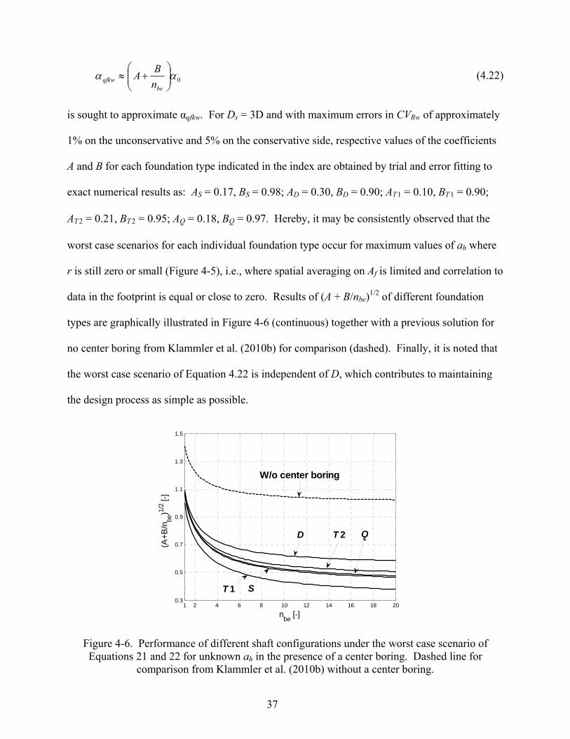
37

0

beqfkw n

BA (4.22)

is sought to approximate αqfkw. For Ds = 3D and with maximum errors in CVRw of approximately

1% on the unconservative and 5% on the conservative side, respective values of the coefficients

A and B for each foundation type indicated in the index are obtained by trial and error fitting to

exact numerical results as: AS = 0.17, BS = 0.98; AD = 0.30, BD = 0.90; AT 1 = 0.10, BT 1 = 0.90;

AT 2= 0.21, BT 2 = 0.95; AQ = 0.18, BQ = 0.97. Hereby, it may be consistently observed that the

worst case scenarios for each individual foundation type occur for maximum values of ah where

r is still zero or small (Figure 4-5), i.e., where spatial averaging on Af is limited and correlation to

data in the footprint is equal or close to zero. Results of (A + B/nbe)1/2 of different foundation

types are graphically illustrated in Figure 4-6 (continuous) together with a previous solution for

no center boring from Klammler et al. (2010b) for comparison (dashed). Finally, it is noted that

the worst case scenario of Equation 4.22 is independent of D, which contributes to maintaining

the design process as simple as possible.

1 2 4 6 8 10 12 14 16 18 200.3

0.5

0.7

0.9

1.1

1.3

1.5

nbe

[-]

(A+

B/n

be)1/

2 [-]

T1 S

QT2D

W/o center boring

Figure 4-6. Performance of different shaft configurations under the worst case scenario of Equations 21 and 22 for unknown ah in the presence of a center boring. Dashed line for

comparison from Klammler et al. (2010b) without a center boring.

S

D QT 2

T 1

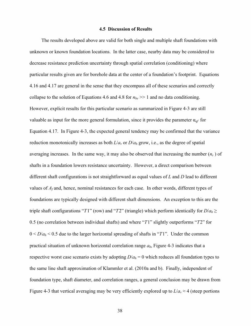
38

4.5 Discussion of Results

The results developed above are valid for both single and multiple shaft foundations with

unknown or known foundation locations. In the latter case, nearby data may be considered to

decrease resistance prediction uncertainty through spatial correlation (conditioning) where

particular results given are for borehole data at the center of a foundation’s footprint. Equations

4.16 and 4.17 are general in the sense that they encompass all of these scenarios and correctly

collapse to the solution of Equations 4.6 and 4.8 for nbe >> 1 and no data conditioning.

However, explicit results for this particular scenario as summarized in Figure 4-3 are still

valuable as input for the more general formulation, since it provides the parameter αqf for

Equation 4.17. In Figure 4-3, the expected general tendency may be confirmed that the variance

reduction monotonically increases as both L/av or D/ah grow, i.e., as the degree of spatial

averaging increases. In the same way, it may also be observed that increasing the number (ns ) of

shafts in a foundation lowers resistance uncertainty. However, a direct comparison between

different shaft configurations is not straightforward as equal values of L and D lead to different

values of Af and, hence, nominal resistances for each case. In other words, different types of

foundations are typically designed with different shaft dimensions. An exception to this are the

triple shaft configurations “T1” (row) and “T2” (triangle) which perform identically for D/ah ≥

0.5 (no correlation between individual shafts) and where “T1” slightly outperforms “T2” for

0<D/ah < 0.5 due to the larger horizontal spreading of shafts in “T1”. Under the common

practical situation of unknown horizontal correlation range ah, Figure 4-3 indicates that a

respective worst case scenario exists by adopting D/ah = 0 which reduces all foundation types to

the same line shaft approximation of Klammler et al. (2010a and b). Finally, independent of

foundation type, shaft diameter, and correlation ranges, a general conclusion may be drawn from

Figure 4-3 that vertical averaging may be very efficiently explored up to L/av ≈ 4 (steep portions

39

of curves), while for L/av > 4 the benefits of increasing shaft length on uncertainty reduction (in

absolute terms) become small.

As reflected by Equations 4.17 or 4.22, the latter conclusion remains valid in the presence

of a center boring in the footprint of a single or multiple shaft foundation. Moreover, a center

boring has the benefit of leading to considerably more favorable worst case scenarios for

unknown ah as reflected by Figure 4-6 where continuous graphs correspond to results from

Equation 4.22 and the dashed line represents (1 + 1/nbe)1/2 as derived in Klammler et al. (2010b)

for an unknown foundation location (i.e., no center boring). This remains true even if no actual

data conditioning between the center boring and the foundation exists (i.e., r = 0, such as

considered for unknown foundation location) which is due to the mere fact that data was

collected inside the foundation footprint and used in Equation 4.16. Figure 4-6 demonstrates that

for a given number of borings nbe, the benefit of a center boring is a 50% reduction in CVR.

Provided a center boring is available, Figure 4-6 also illustrates the performance of different

shaft configurations in terms of resistance uncertainty. As above, a direct comparison is not

straightforward due to generally different shaft dimensions for each configuration, but assuming

equal L/av (i.e., α0 in Equation 4.22) some observations may be made. Independent of nbe, the

configuration “T1” (triple row) performs clearly best among all foundation types considered.

“T1” is followed by “S” (single), “Q” (quadruple) and “T2” (triple triangle) which show similar

behaviors and, finally, “D1” (double). The perhaps unexpectedly good performance of “T1”

may be attributed to the fact that the center boring falls exactly into the footprint of the center

shaft, which reduces uncertainty substantially. In other words, data conditioning starts at lower

ah (compare Figure 4-5) when horizontal averaging is still more effective as well. Another

interesting observation from Figure 4-6 is that prediction uncertainty may be efficiently reduced

up to nbe ≈ 4 (steep portions of graphs), while for nbe > 4 the benefit of additional borings on

40

uncertainty reduction decreases. This fact is very important for sites which are not statistically

homogenous, i.e., where (horizontal) division into sub-zones is required for separate

geostatistical treatment such that the nbe for each sub-zone become smaller (e.g., 5 instead of 15).

Moreover, in the (actual or potential) presence of smooth horizontal trends over a site, nbe may

be limited without significantly inflating uncertainty to a small number of nearest borings which

are used for design of a foundation (“moving window approach,” Journel and Rossi 1989). This

may avoid making crucial decisions about the presence and shape of horizontal deterministic

trend functions. Finally, in the presence of vertical layering and/or nested variogram structures,

the approach of Klammler et al. (2010a) remains valid which is based on separate treatment of

individual layers and/or variogram components with subsequent addition of predictions and

prediction variances.

4.6 Practical Example

In order to demonstrate the application of the results presented, the 17th Street Bridge case

study of Klammler et al. (2010a) is extended by considering a triangle (“T2”) foundation with

L= 9 m, D = 0.4 m and the presence or not of a center boring. A total of 136 local rock strength

measurements from 6 borings is available, where qbm = 2.28 MPa with CVq = 0.50. A spherical

covariance function is adopted with correlation ranges of av = 1.5 m and ah = 4.5 m for 80% of

2q plus av = ∞ and ah = 4.5 m for the remaining 20% (i.e., 20% of the variability in q is only

contained in the horizontal direction — “random areal trend.” For the purpose of illustrating the

present approach, the 6 borings are assumed spatially uncorrelated among each other such that

neb = 6.

In a first design step with unknown foundation location or before obtaining data from a

center boring Rn = Af qbm = 77.31 MN, where Af = 3·0.4·π·9 = 33.91 m2. Assuming ah and,

41

consequently, D/ah = 0.4/4.5 = 0.09 are known, Figure 4-3 immediately gives a variance

reduction factor for the first variogram component with L/av = 9/1.5 = 6 of αqf1 = 0.312 and for

the second variogram component with L/av = 9/∞ = 0 of αqf2 = 0.842. Applying a result of

Klammler et al. (2010a) αqf1 and αqf2 may be combined to a total variance reduction factor by

taking the weighted average αqf = 0.8αqf1 + 0.2αqf2 = 0.22 such that further CVR = 0.221/2 · 0.5

=0.23 and Φ = 0.63 from Equation 4.10 (ΦRn = 48.71 MN). In case ah is not reliably known,

the same chart of Figure 4-3 gives worst case values of α01 = 0.352 and α02 = 1 by using D/ah = 0.

By the same relationships from above this leads to α0 = 0.30, CVR = 0.27 and a reduced Φ = 0.56

(ΦRn = 43.29 MN). These results are very similar to those obtained for a single shaft in

Klammler et al. (2010a) which may be attributed to the reduced shaft diameter for the triple

configuration in order to achieve equal Rn.

In a more advanced stage of the design process, data from a center boring at a foundation

location may be available. Assuming that ah is known and that the mean local strength observed

in the center boring is qb1 = 1.70 MPa, respective values of r1 = 0.87 (continuous line for

L/av=6> 1) and r2 = 0.77 (dashed line for L/av = 0) are obtained from Figure 4-5 which may be

combined by the same process of variance weighted averaging to a total value of r = 0.8r1+0.2r2

= 0.85. Equations 4.16 and 4.18 then give ff = 0.85 · 1.70 + 0.15 · 2.28 = 1.79 MPa and

Rn=33.91 · 1.79 = 60.70 MN. Furthermore, Equation 4.17 may be evaluated with all

parameters known from above as 1/ 2qfk = [0.30(0.152/6 – 0.852) + 0.22]1/2 = 0.07. Equation 4.19

then gives CVR = 0.07 · 0.5/(1 – 0.25 · 0.85) = 0.044 which translates into Φ = 0.98 by Equation

4.10 such that ΦRn = 59.49 MN. This is significantly larger than 48.71 MN obtained above in

the absence of a center boring and with known ah = 4.5 m even though Rn is 25% smaller.

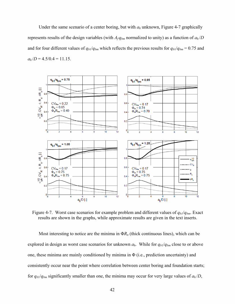
42

Under the same scenario of a center boring, but with ah unknown, Figure 4-7 graphically

represents results of the design variables (with Af qbm normalized to unity) as a function of ah /D

and for four different values of qb1/qbm which reflects the previous results for qb1/qbm = 0.75 and

ah /D = 4.5/0.4 = 11.15.

Figure 4-7. Worst case scenarios for example problem and different values of qb1/qbm. Exact results are shown in the graphs, while approximate results are given in the text inserts.

Most interesting to notice are the minima in ΦRn (thick continuous lines), which can be

explored in design as worst case scenarios for unknown ah. While for qb1/qbm close to or above

one, these minima are mainly conditioned by minima in Φ (i.e., prediction uncertainty) and

consistently occur near the point where correlation between center boring and foundation starts;

for qb1/qbm significantly smaller than one, the minima may occur for very large values of ah /D,

43

thus being conditioned by small values of Rn without significant prediction uncertainty

(CVR≈0). In the above case of qb1/qbm = 0.75, for example, ΦRn=0.73Afqbm = 56.44 MN is

obtained being only slightly smaller than 59.49 MN for ah = 4.5 m from above. As evident from

Figure 4-7, the potential increase in ΦRn due to a known ah becomes larger as qb1/qbm grows.

Considering only worst case scenarios, however, benefits in ΦRn due to larger qb1/qbm (i.e.,

stronger ground at the foundation location) are not very significant in the present case. An

improvement upon the minima in ΦRn of Figure 4-7 can be possible by explicitly taking into

account the spatial correlation structures between all borings (i.e., improving on the conservative

assumption that two nearby borings are fully correlated) and by allowing for correlation between

more than a single boring with the foundation. However, this would quickly lead to an increased

computational complexity, since an ordinary kriging system has to be solved for every value of

ah/D instead of the simplified Equations 4.16 and 4.17. Even evaluation of worst case scenarios

as in Figure 4-7 based on Equations 4.16 and 4.17 may soon become a tedious task without

computational aid and even more conservative worst case scenarios are indicated inside the

charts based on the approximate Equations 4.20, 4.21 and 4.22. For the example problem with

qb1/qbm = 0.75, this results in Rnw = 0.75Afqbm = 57.99 MN, αqfkw = (0.21 + 0.95/6)·0.30 = 0.11,

CVRw = 0.111/2·0.5 / 0.75 = 0.22, Φw = 0.65 and ΦwRnw = 37.69 MN, which presents a relatively

large decrease in admissible load with respect to 56.44 MN from above based on simultaneous

minimization of the product ΦRn rather than of each factor separately. However, as illustrated by

Figure 4-7, this conservative difference decreases quickly as qb1/qbm approaches or exceeds unity.

This indicates that an additional mathematical effort to directly minimize the product ΦRn may

be quite compensating, especially for qb1/qbm < 1.

44

CHAPTER 5 UNMONITORED, PARTIALLY AND FULLY MONITORED

PILE GROUPS – KRIGING APPROACH

5.1 Background

The present chapter further generalizes the kriging approach from Chapter 4 for the

particular scenario of partially monitored (including unmonitored and fully monitored) pile

groups. Total pile resistance Rp (i.e., side + tip) is hereby considered as a spatially random

variable, as this avoids individual treatment of side and tip resistances with subsequent addition

(problem of side-tip correlation). Note, this data is generally available from high strain rate pile

monitoring systems and is generally used to set pile lengths, blow counts, etc. For this develop-

ment, the following assumptions are considered:

Data used are total pile resistances such that each pile represents a point location in the

horizontal plane (no more horizontal and vertical averaging over pile surfaces);

Different numbers and configurations of piles may be monitored in a group; and

The number and configuration of monitored piles may be different from group to group.

5.2 List of Variables for Chapter Five

To assist with the description of monitored and unmonitored pile variables, uncertainties,

etc., the following variable descriptions are provided:

i Index from 1 to ng denoting pile groups; i = 1 denotes pile group to be designed such that indexation of i changes depending on what pile group is being designed (refer to Figure 5-2).

j, k Indices from 1 to npi denoting piles in group i; piles from j, k = 1 to nmi are monitored, while piles from j, k = nmi + 1, nmi + 2, …, npi are unmonitored (refer to Figure 5-1).

ng Number of pile groups in a site (homogeneous subzone), where at least one pile is monitored.

npi Number of piles in pile group i.

nmi Number of monitored piles in pile group i.

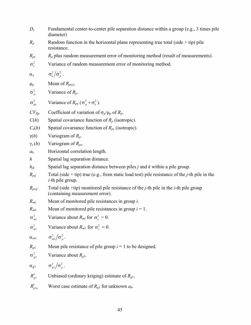
45

Ds Fundamental center-to-center pile separation distance within a group (e.g., 3 times pile diameter)

Rp Random function in the horizontal plane representing true total (side + tip) pile resistance.

Rpε Rp plus random measurement error of monitoring method (result of measurements). 2 Variance of random measurement error of monitoring method.

ε 2 2

p .

μp Mean of Rp(ε). 2p Variance of Rp.

2p Variance of Rpε (

2 2p ).

CVRp Coefficient of variation of p/μp of Rp.

C(h) Spatial covariance function of Rp (isotropic).

Cε(h) Spatial covariance function of Rpε (isotropic).

(h) Variogram of Rp.

γε (h) Variogram of Rpε.

ah Horizontal correlation length.

h Spatial lag separation distance.

hjk Spatial lag separation distance between piles j and k within a pile group.

Rpij Total (side + tip) true (e.g., from static load test) pile resistance of the j-th pile in the i-th pile group.

Rpεij Total (side +tip) monitored pile resistance of the j-th pile in the i-th pile group (containing measurement error).

Rmi Mean of monitored pile resistances in group i.

Rm1 Mean of monitored pile resistances in group i = 1. 2mi Variance about Rmi for 2

= 0.

21m Variance about Rm1 for 2

= 0.

m1 2 2

1 .m p

Rg1 Mean pile resistance of pile group i = 1 to be designed. 2

1g Variance about Rg1.

g1 2 2

1 .g p

1gR Unbiased (ordinary kriging) estimate of Rg1.

1g wR Worst case estimate of Rg1 for unknown ah.

46

Rn Nominal LRFD resistance given by np1 1gR or np1 1 .g wR

wi Ordinary kriging weights of all Rmi.

W1 Weight of Rm1 against μp.

W1min Minimum value of W1 for unknown ah.

W1max Maximum value of W1 for unknown ah.

Lagrangian operator. 2

1mg Covariance between Rm1 and Rg1.

mg1 2 2

1 .mg p

2e Variance of estimation error 1 1g gR R .

e 2 2 .e p

αew Worst case value of αe for unknown ah.

CVRg1 Coefficient of variation of estimation error 1e gR = 1/ 2e CVRp for finding Φ.

CVRg1w Worst case value of CVRg1w for unknown ah.

Φ LRFD resistance factor for pile group i = 1 (Q < 1 ( )g wR ).

Φw Worst case Φ for unknown ah.

Q Mean of random design load for pile group i = 1.

Qw Worst case Q for unknown ah.

β LRFD reliability index.

5.3 Predicting Pile Group Resistance from Monitored Piles Using Kriging

It is common practice in pile driving that once the minimum tip elevation is reached (e.g.,

for lateral load requirements) then final unmonitored pile lengths are set by the hammer blow

count. If all piles are driven to the (approximately) same number of hammer blows per foot with

approximately the same embedment depth, then the total pile resistance Rp may be considered as

a random function in the horizontal plane. Randomization of Rp is due to uncertainties of the

“hammer blow count approach” (or spatial variability of Rp for constant embedment depth),

which may or may not depend on the spatial soil properties. As such, Rp may or may not be

spatially correlated and sampled values of Rp are available as Rpεij at monitored pile locations,

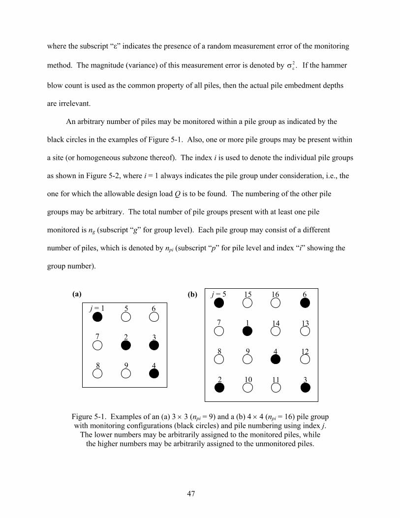
47

where the subscript “ε” indicates the presence of a random measurement error of the monitoring

method. The magnitude (variance) of this measurement error is denoted by 2. If the hammer

blow count is used as the common property of all piles, then the actual pile embedment depths

are irrelevant.

An arbitrary number of piles may be monitored within a pile group as indicated by the

black circles in the examples of Figure 5-1. Also, one or more pile groups may be present within

a site (or homogeneous subzone thereof). The index i is used to denote the individual pile groups

as shown in Figure 5-2, where i = 1 always indicates the pile group under consideration, i.e., the

one for which the allowable design load Q is to be found. The numbering of the other pile

groups may be arbitrary. The total number of pile groups present with at least one pile

monitored is ng (subscript “g” for group level). Each pile group may consist of a different

number of piles, which is denoted by npi (subscript “p” for pile level and index “i” showing the

group number).

Figure 5-1. Examples of an (a) 3 3 (npi = 9) and a (b) 4 4 (npi = 16) pile group with monitoring configurations (black circles) and pile numbering using index j.

The lower numbers may be arbitrarily assigned to the monitored piles, while the higher numbers may be arbitrarily assigned to the unmonitored piles.

j = 1

2 3

4

5 6

7

8 9

j = 5

1 14

4

15 16

7

8 9

13

12

6

11 2 10 3

(a) (b)

48

Figure 5-2. (a) Example of pile groups and monitoring configurations (black circles) for ng = 4

(Term i=1 is used for the pile group under consideration, while i > 1 may be arbitrarily assigned to the other pile groups); (b) Simplified model corresponding to Equation 5.9.

Rpij stands for the total true (i.e., without measurement error, e.g., from static load test)

resistance of the j-th pile in the i-th pile group. The numbering of piles within a group may be

arbitrary with the exception that the lower indices are assigned to monitored piles, while the

higher indices are assigned to unmonitored piles. Using nmi as the number of monitored piles in

the i-th group (subscript “m” for monitored and index “i” again for group number), this means

that j = 1, 2, …, nmi indicate monitored piles, while j = nmi + 1, nmi + 2, …, npi indicate

unmonitored piles (compare Figure 5-1).

The true pile resistance mean Rg1 in the pile group of interest (i = 1) is given by

1

11

11

1 pn

jjp

pg R

nR (5.1)

i = 1 (to be designed)

i = 2

i = 3

i = 4

2 2 21 1 1, ,m g mg

(a)

i = 1

(b)

i = 2 i = 3

i = 4

22m

23m

24m

2p 2

p

2p 2 2 2

1 1 1, ,m g mg

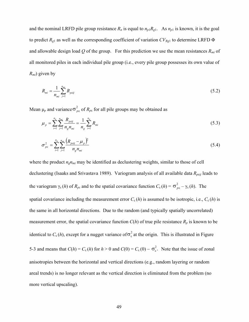
49

and the nominal LRFD pile group resistance Rn is equal to np1Rg1. As np1 is known, it is the goal

to predict Rg1 as well as the corresponding coefficient of variation CVRg1 to determine LRFD Φ

and allowable design load Q of the group. For this prediction we use the mean resistances Rmi of

all monitored piles in each individual pile group (i.e., every pile group possesses its own value of

Rmi) given by

min

jijp

mimi R

nR

1

1 (5.2)

Mean μp and variance2p of Rpε for all pile groups may be obtained as

gg mi n

imi

g

n

i

n

j mig

ijpp R

nnn

R

11 1

1 (5.3)

g min

i

n

j mig

pijpp nn

R

1 1

2

2

(5.4)

where the product ngnmi may be identified as declustering weights, similar to those of cell

declustering (Isaaks and Srivastava 1989). Variogram analysis of all available data Rpεij leads to

the variogram γε (h) of Rpε and to the spatial covariance function Cε (h) = 2p – γε (h). The

spatial covariance including the measurement error Cε (h) is assumed to be isotropic, i.e., Cε (h) is

the same in all horizontal directions. Due to the random (and typically spatially uncorrelated)

measurement error, the spatial covariance function C(h) of true pile resistance Rp is known to be

identical to Cε(h), except for a nugget variance of 2 at the origin. This is illustrated in Figure

5-3 and means that C(h) = Cε (h) for h > 0 and C(0) = Cε (0) 2. Note that the issue of zonal

anisotropies between the horizontal and vertical directions (e.g., random layering or random

areal trends) is no longer relevant as the vertical direction is eliminated from the problem (no

more vertical upscaling).

50

Figure 5-3. Difference between Cε (h) and C(h). Cε (h) and C(h) are identical

except for Cε (0) = 2p and C(0) =

2p .

Using ordinary kriging, Rg1 may be predicted from known Rmi as

11

gn

g i mii

R w R

(5.5)

where the sum of the kriging weights 11

gn

iiw . Under the assumption that C(h) = 0 between

different pile groups (i.e., possible spatial correlation only within pile groups), wi are found from

the ordinary kriging system,

1

0

0

011

100

0

0

100 21

2

1

22

2

22

2

1

22

1

mg

ng

mngmng

mm

mm

w

w

w

n

n

n

(5.6)

with

mi min

j

n

kjk

mimi hC

n 1 12

2 )(1 (5.7)

h

(b) C(h)

0 ah

(a)

2p

h

Cε(h)

0

2

2p

2p

ah

51

1 1

1 111

21 )(

1 m pn

j

n

kjk

mpmg hC

nn (5.8)

where hjk is the lag distance between the j-th and k-th piles in the i-th group and μ is the

Lagrangian operator. Equation 5.7 represents nothing but the mean value of C(h) between all

possible pairs of monitored piles, which is identical to the mean of all elements in the variance–

covariance matrix between all monitored piles in group i. In analogy, Equation 5.8 is nothing

but the mean value of C(h) between all possible pairs of a monitored pile in the 1st group and

every pile (both monitored and unmonitored) in the 1st group. As such, for the example of

Figure 5-1a, Equation 5.7 corresponds to averaging over the darkly shaded portion of the

variance–covariance matrix depicted in Figure 5-4 while Equation 5.8 corresponds to averaging

over both the darkly and lightly shaded portions.

In order to simplify Equation 5.6 and to arrive at a closed form solution, it is assumed in

Equation 5.7 that spatial correlation within the groups is large enough, such that

C(hjk) ≈ C(0)= 2p can be used for i > 1 leading to Figure 5-2b and

1

0

0

011

100

0

0

100 21

2

2

1

22

22

1

22

1

mg

p

p

mm

w

w

wn

(5.9)

52

Monitored Unmonitored

j 1 2 3 4 5 6 7 8 9

Mon

itor

ed 1 C11 C12 C13 C14 C15 C16 C17 C18 C19

2 C21 C22 C23 C24 C25 C26 C27 C28 C29

3 C31 C32 C33 C34 C35 C36 C37 C38 C39

4 C41 C42 C43 C44 C45 C46 C47 C48 C49

Unm

onit

ored

5 C51 C52 C53 C54 C55 C56 C57 C58 C59

6 C61 C62 C63 C64 C65 C66 C67 C68 C69

7 C71 C72 C73 C74 C75 C76 C77 C78 C79

8 C81 C82 C83 C84 C85 C86 C87 C88 C89

9 C91 C92 C93 C94 C95 C96 C97 C98 C99

Figure 5-4. Variance–covariance matrix between all piles of the example in Figure 5-1a (npi = 9 and nmi = 4). Index j is bold and Cjk is short for C(hjk). The mean of all elements in the darkly

shaded portion corresponds to Equation 5.7. The mean of all elements in the darkly and lightly shaded portions corresponds to Equation 5.8. The mean

of all 9 9 elements corresponds to Equation 5.16. This is equivalent to increasing the uncertainty about the data values from all pile groups, except

the one of interest (i = 1). As a consequence, this results in a larger uncertainty about the final

group resistance estimate as well as a higher kriging weight for Rm1 (whose variance is not

increased). Equation 5.9 may be expanded into the following set of equations:

22 2

1 1 11

2 22

1 2

0

1 1

m mgm

p

g

wn

w

w n w

(5.10)

Note that wi = w2 for i > 1. Solving for w1, w2 and μ gives

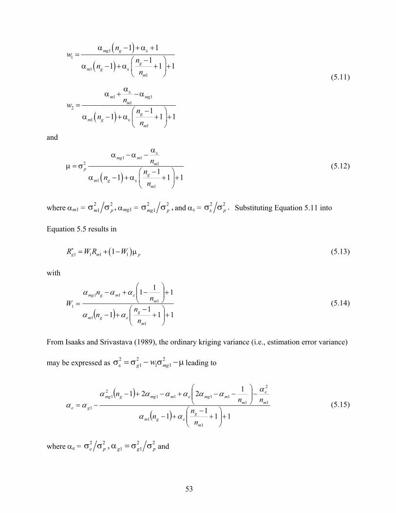
53

1

1

11

1 11

2

11

1 1

11 1 1

11 1 1

mg g

gm g

m

m mgm

gm g

m

nw

nn

n

nw

nn

n

(5.11)

and

1 12 1

11

11 1 1

mg mm

pg

m gm

n

nn

n

(5.12)

where m1 = 2 2

1 ,m p mg1 = 2 2

1 ,mg p and ε = 2 2 .p Substituting Equation 5.11 into

Equation 5.5 results in

1 1 1 11g m pR W R W (5.13)

with

111

1

11

1

11

111

1

m

ggm

mmgmg

n

nn

nn

W

(5.14)

From Isaaks and Srivastava (1989), the ordinary kriging variance (i.e., estimation error variance)

may be expressed as 2 2 2

1 1 1g mgw leading to

111

1

1221

11

1

2

11111

21

1

m

ggm

mmmmgmmggmg

ge

n

nn

nnn

(5.15)

where e = 2 2 2 2

1 1,e p g g p and

54

1 1

1 12

1

21 )(

1 p pn

j

n

kjk

pg hC

n (5.16)

Equation 5.16 is nothing but the mean value of C(h) over all possible pairs of piles (both

monitored and unmonitored) in the 1st pile group. For the example of Figure 5-1a, this is

equivalent to the averaging of all elements of the variance–covariance matrix in Figure 5-4.

5.4 Discussion of Results 5.4.1 No Pile Monitored in Group of Interest (nm1 = 0)

It may occur that none of the piles in a group is monitored, such that nm1 = 0. This leads to

the non-existence of the first rows in Equations 5.6, 5.9 and 5.10 and to

1

12

gnw (5.17)

1

11

gge n

(5.18)

in Equations 5.11 and 5.15. This means that all the available data from other ng – 1 pile groups

is evenly weighted and 1gR= μp; αe collapses to the form for the scenario where limited data is

available and none of them is nearby for conditioning; ng has to be larger than one in this case,

as no data is available from the first pile group. Limits for αε = 0 and ng >> 1 + αε are easily

found from Equation 5.18.

5.4.2 One Pile Monitored in Group of Interest (nm1 = 1)

In case a single pile is monitored in the group of interest, such that nm1 = 1, Equations 5.14

and 5.15 become

1

11

mgW (5.19)

55

gg

gmgmg

gge nn

n

n

2

1

11 111

(5.20)

since αm1 = 1. If in addition np1 >> 1 (i.e., a single pile monitored out of many piles in a group),

then mg1 ≈ 0 and Equation 5.13 yields 1gR≈ μp, which reflects a low degree of monitoring and

uniform weighting of data from all pile groups. Equation 5.20 then becomes αe ≈ αg1 + (1 +

αε)/ng. In the presence of a single pile group, i.e., ng = 1, αe = αg1 + 1 + αε - 2mg1. Note that W1

is not a function of ng in this case (this can be shown to be generally the case when the same

number and pattern of piles is monitored in each group) and that it decreases as αε increases.

That is, the larger the measurement errors, the more uniformly kriging weights are distributed

over all data and 1gR ≈ μp. For αε = 0, Equation 5.20 yields αe = αg1 + 1/ng - mg1[mg1(ng - 1)/ng +

2/ng] and for ng >> 1 ,2

1 1 (1 ).e g mg

5.4.3 All Piles Monitored in Group of Interest (nm1 = np1 )

Here, m1 = mg1 = αg1 and Equations 5.14 and 5.15 become

111

1

11

11

11

111

1

111

1

11

11

p

g

pgm

p

g

p

ggm

pgm

n

n

nn

n

n

n

nn

nn

W

(5.21)

111

11

1

1111

11

1

p

g

pgm

pg

p

m

e

n

n

nn

nn

n

(5.22)

For ng = 1 this gives αe = αε /np1, while for ng >> 1 + αε one finds W1 = αm1/(αm1 + αε /np1)

and αe = αεαm1/(np1αm1 + αε). In the theoretical scenario of no measurement error (αε = 0)

Equations 5.21 and 5.22 reduce to W1 = 1 and αe = 0.

56

In case αε >> 1, αe has to become very large, independent of the particular scenario and all

other parameters. Moreover for ng = 1, i.e., in the presence of a single pile group, 1gR = 1mR = μp

always independent of W1.

5.4.4 Single Pile Group without Spatial Correlation (ng = 1 and ah = 0)

In this case, only monitored data from the pile group of interest is considered, except for

CVRp which may be based on all monitored data at a site. Thus, Equation 5.13 becomes

1 1g mR R independent of ah, which may be unconservative for pile groups where Rm1 > μp. In

the hypothetical case that both ng = 1 and ah = 0 (such that αg1 = αmg1 = 1/np1 and αm1 = 1/nm1),

Equation 5.15 reduces to the simple form,

11

11

pme nn

(5.23)

This nicely illustrates how αe grows with αε and np1 and how it decreases with nm1. However, as

seen later in Figures 5-9b and 5-10b (top continuous graphs of each color), the case of ah = 0 is

not a universal worst case scenario.

5.5 Worst Case Scenarios of Unknown ah

The behavior of W1 from Equation 5.15 is graphically illustrated by the dashed lines in

Figures 5-5 through 5-10, where black, blue and red correspond to αε = 2 2

pCV CV = {0, 0.1,

0,3}. Black circles in the pile groups indicate the monitored piles and Ds is an arbitrary

fundamental pile separation distance (center-to-center; e.g., Ds = 3 times pile diameter). From

top to bottom, the dashed lines correspond to ng = {1, 5, 100}, i.e., the larger ng the larger the

weight on μp in Equation 5.14. Moreover, it may be observed that W1 possesses a minimum

value W1min and a maximum value W1max at ah /Ds >> 1. The latter may be generally expressed as

57

1111

max1

mgmg

g

nnnn

nW

(5.24)

while a simple equation for the former may only be found for the configurations of Figures 5-5

through 5-8 where W1min consistently occurs at ah /Ds < 1. Since in these cases W1min occurs

when there is no more correlation between individual piles in the group, Equations 5.7, 5.8 and

5.16 simplify leading to g1 = mg1 = 1/np1, m1 = 1/nm1 and

1

1

11 1

1

1

1

1

min1

mg

m

mg

gp

m

nn

n

nn

nn

n

W

(5.25)

Figure 5-5. Terms W1 (dashed, except for (a), where W1 does not exist as no pile is monitored in the group) and e (continuous) as functions of ah /Ds from Equations 5.14 and 5.15 for a double

pile group. Black circles indicate monitored piles. Colors black, blue and red correspond to αε = {0, 0.1, 0.3}, respectively. For each color and line type there are three graphs corresponding to ng = {1, 5, 100} from top to bottom, except for (a) where ng = {2, 5, 100}. Graphs for W1 and

different ng are identical whenever nm1 = 1 (compare Equation 5.19).

58

Figure 5-6. Analogous to Figure 5-5 for tripe pile groups in a line and different monitoring configurations.

59

Figure 5-7. Analogous to Figure 5-5 for tripe pile groups in a triangle and different monitoring configurations.

60

Figure 5-8. Analogous to Figure 5-5 for 2 2 pile groups and different monitoring configurations.

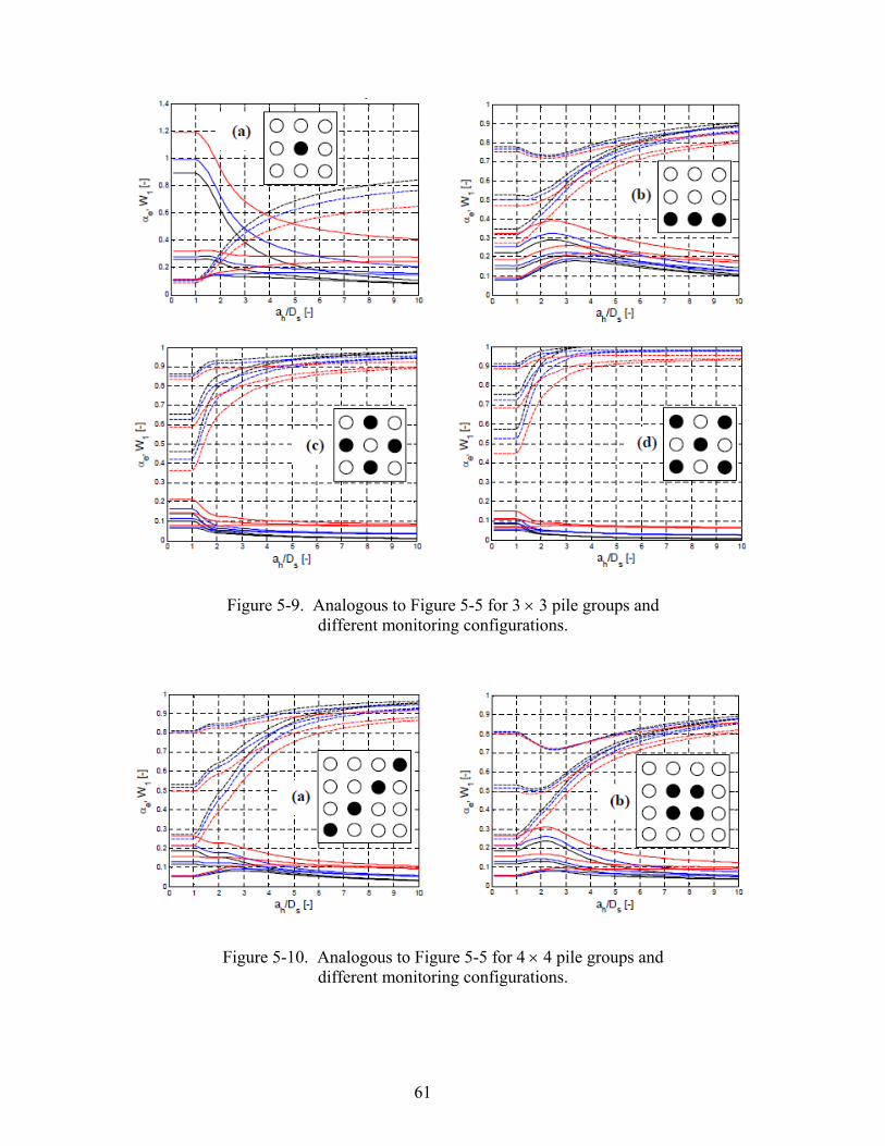
61



62

In more complex configurations of Figures 5-9 and 5-10, minima in W1 may occur at

different locations and are best determined graphically. In case ah is not available for explicit

computation of W1, a worst case prediction 1g wRmay hence be defined as

1 1max 1 1max 1min 1 1minmin 1 , 1g w m p m pR W R W W R W (5.26)

In other words, 1g wR = W1maxRm1 + (1-W1max)μp if Rm1 ≤ μp, and 1g wR

= W1minRm1 + (1-W1min)μp,

if Rm1 > μp. This shows that for an increasing degree of monitoring (i.e., nm1 → np1) W1min

approaches ng + (nm1 - 1)(1 + αε)/[(ng + nm1 - 1)(1 + αε)] which is one for αε = 0, such that the

worst case prediction 1g wRapproaches Rm1. With nm1 = 1, Equation 5.25 collapses to

W1min=1/[np1(1 + αε)], while for large ng it may be found that W1min = nm1/[np1(1 + αε)].

For computation of LRFD Φ (e.g., through AASHTO, Equation 4.10, assuming log-normal

distributions of load and resistance), CVRg1 is required which may be found from Equation 5.15

by CVRg1 = 1/ 2e CVRp, where CVRp = p /μp. For ng = 1, Equation 5.15 collapses to

e=g1+m12mg1, while for large ng, e ≈ g1 2

1 1 .mg m Although a mathematical

model for C(h), e.g., spherical or exponential, may be adopted to find closed form expressions of

Equations 5.7 through 5.16 by simple algebraic manipulations, this process is extremely lengthy,

needing to be repeated for every single combination of pile group type and monitoring

configuration. Useful (i.e., sufficiently short /simple) results for practical application are not

expected. Instead, in the same way as W1 from Equation 5.14, Equation 5.15 is evaluated

numerically and results are investigated graphically for several example configurations in

Figures 5-5 through 5-10 (continuous lines). From top to bottom, the lines correspond to

ng={1,5, 100}, i.e., the larger ng the smaller αe and the larger will be Φ. Black, blue and red

63

again correspond to αε = 2 2

pCV CV = {0, 0.1, 0.3} where larger values of αε clearly lead to

larger uncertainty and αe.

It may be observed that, in general, an increase in the number nmi of monitored piles leads

to a more substantial reduction in αe than a comparable increase in the number ng of pile groups.

This is, the number of data available outside the pile group of interest is less important than the

number of data available within the pile group of interest. This is further reflected by the fact

that as ah /Ds grows, αe becomes increasingly independent of ng. It is also observed that it is

advantageous to locate monitored piles near the center of pile groups (compare Figures 5-6a and

5-6b) as well as not immediately adjacent to each other (compare Figures 5-6c and 5-6d as well

as Figures 5-8b and 5-8c). Worst case values ew for unknown ah are seen to mostly occur at

ah/Ds ≤ 1, i.e., when no correlation is present between individual piles. However, exceptions are

when ng is large and nm1 is small, such that “humps” in the graphs become evident at ah /Ds ≈ 2.

Unfortunately, these humps become more pronounced as αε > 0 and ew is best determined

graphically.


To better illustrate the outcome and implications of the previous section, an example is

worked. Consider a bridge site with five pile groups (ng), where for the group of interest (i=1, or

group 1) the number of piles monitored (nm1) are 1, 2, or 3, and the mean of the monitored pile

resistance (Rm1) of group 1 is 1.6 MN as given,

μp = 2 MN CVRp = 0.5 Rm1 = 1.6 MN ε = 0 C(h) is spherical with ah /Ds = 3 ng = 5 Square pile group with nm1 = 1, 2, 3 Reliability index β = 3

64

e

CV

Rp

1/2

n p1

Rg1

ew

CV

Rp

1/2

n p1

Rg1

w

Given in Table 5-1 are the results where italic numbers are read from the respective

figures. It may be observed that Φ consistently grows as nm1 increases. However, the variable of

ultimate interest, the design load Q(w), also depends on the ratio Rm1/μp and general conclusions

are hence more difficult to make. Finally, it is noted that the present worst case investigation is

based on a separate minimization of 1gRand Φ. In cases where the two minima do not occur at

equal values of ah /Ds (e.g., in the present scenario 1g wRis obtained at ah /Ds >> 1 and αew at

ah/Ds ≈ 1), a more favorable worst case design load Qw may be obtained by direct (numerical)

minimization of the product Φ 1gRas a function of ah /Ds (as shown in Chapter 4). This is

equivalent to assuming different possible values of ah and finding respective values of Q from

which the minimum is chosen as Qw. It is recalled that the resistance Q represents the entire pile

group.

Table 5-1. Summary of Results from Practical Example.

nm1 Fig. W1 1gR αe CVRg1 Φ Q W1min 1g wR

αew CVRg1w Φw Qw

- - - MN - - - MN - MN - - - MN 1 5-7a 0.60 1.76 0.28 0.26 0.59 4.16 0.25 1.6 0.31 0.28 0.54 3.46 2 5-7b 0.79 1.68 0.13 0.18 0.72 4.84 0.58 1.6 0.18 0.21 0.67 2.28 2 5-7c 0.89 1.64 0.08 0.14 0.80 5.26 0.58 1.6 0.17 0.21 0.67 2.28 3 5-7d 0.94 1.62 0.04 0.10 0.89 5.78 0.82 1.6 0.08 0.14 0.80 5.12

Eqn

. 5.1

3

AA

SH

TO

Eqn

. 5.2

5

Eqn

. 5.2

6

A

AS

HT

O

65

CHAPTER 6 UNMONITORED, PARTIALLY AND FULLY MONITORED PILE

GROUPS – REGRESSION APPROACH

6.1 Background

The previous two chapters consider estimation of driven pile group resistance and

uncertainty based on SPT/CPT data (for side friction only) and directly monitored data (EDC,

PDA; side + tip resistance). Fundamental assumptions in both cases are that SPT/CPT estimates

of local strength in the former case and monitored pile resistances in the latter case may be

regarded as random functions in space. As such, the approach in Chapter 5 requires some

common characteristic of all monitored and unmonitored piles (e.g., equal embedment depths or

blow counts). This may be in accordance with design practice if other load scenarios other than

pure axial load are dominant (e.g., lateral loading requiring minimum embedment depth). In

general, however, piles are driven until a desired design resistance is reached with the number of

hammer blow counts, i.e., blows/ft, etc., varying from pile to pile. Beside this, the use of

SPT/CPT data (i.e., Chapter 4) from the design phase prior to any (test) for pile

driving/monitoring introduces more complexity.

Due to the conceptual limitations (i.e., equal pile capacity/blows) of Chapter 5 and added

complexity of SPT/CPT data of Chapter 4, the present chapter seeks an alternative solution based

on two modifications: (1) Blow count data during pile installations is incorporated as an

additional piece of information to more closely emulate construction practice; and (2)spatial

correlation between monitored pile resistances is neglected to avoid conceptual limitations

(approach more flexible/adaptive to different design situations) and to make results more

designer friendly. As such, Chapters 5 and 6 may be regarded as two particular simplifications

of a general co-kriging approach, which would consider monitored pile resistances and pile blow

count data as primary and secondary variables, respectively. While Chapter 5 neglects the

66

collocated secondary variable (blow counts are ignored), Chapter 6 neglects spatial correlation of

the primary variable (spatial correlation of monitored resistances is ignored). Since blow count

data is known to be well correlated with “true” resistances from static load tests (and, hence, also

with monitored pile resistances), the loss of information (increase in uncertainty) through

neglecting spatial correlation of monitored resistances is quite insignificant (see Appendix for an

illustrative example). Before developing the approach, an overview is given of different

relationships which have been used between blow counts and pile capacities.

6.2 Examples of Relationships between Blow Count and Pile Capacities

Relationships between static pile capacity R and hammer blow counts measured during

pile driving go back to the earlier 1800s. Generally, the early relationships were linear and the

later representations were nonlinear (Paikowsky 2004). For instance, one of the most popular

capacity estimations is the Engineering News-Record (ENR) formula by Wellington (Paikowsky

2004),

( )h He W H

RFS s C

(6.1)

where WH is the weight of the hammer ram expressed in the same units as R; eh the energy loss

of the hammer; H the height of fall of the ram (i.e., its stroke); s the pile permanent set; and C the

energy loss per hammer blow. Values H, s and C are in inches, where C = 1 inch for drop

hammers and C = 0.1 inches for all other hammers. FS is a factor of safety, generally ranging

from 2 to 6.

Another popular approach is the FHWA Gates relationship (Paikowsky 2004) expressed as

1.75 log (10 ) 100u HQ W H N (6.2)

67

where Qu is the ultimate pile resistance in kips; WH the weight of the hammer ram in pounds; H

the height of fall of the ram (i.e., its stroke) in feet; and N the driving resistance in blows/inch.

Both approaches are generally used where high strain rate measurement devices are not

employed (Paikowsky 2004). Their characterization of a Delmag D22 (60kip-ft) hammer with

various blow counts is shown in Figure 6-1 (ENR: FS = 4, eh = 0.85). Evident from Figure 6-1,

both approaches are nonlinear; however, the ENR results could be approximated as linear. Also,

both approaches differ the most at low and high blow counts, but both methods would be

characterized as linear in a log-log plot.

Figure 6-1. Comparison of ENR and FHWA-Gates for Delmag D22.

National Cooperative Highway Research Program (NCHRP) Report 507 (Paikowsky

2004) evaluated both approaches with a database of measured versus predicted static resistances.

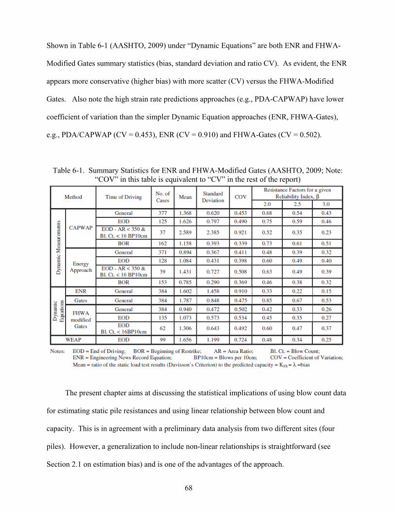
68

Shown in Table 6-1 (AASHTO, 2009) under “Dynamic Equations” are both ENR and FHWA-

Modified Gates summary statistics (bias, standard deviation and ratio CV). As evident, the ENR

appears more conservative (higher bias) with more scatter (CV) versus the FHWA-Modified

Gates. Also note the high strain rate predictions approaches (e.g., PDA-CAPWAP) have lower

coefficient of variation than the simpler Dynamic Equation approaches (ENR, FHWA-Gates),

e.g., PDA/CAPWAP (CV = 0.453), ENR (CV = 0.910) and FHWA-Gates (CV = 0.502).

Table 6-1. Summary Statistics for ENR and FHWA-Modified Gates (AASHTO, 2009; Note: “COV” in this table is equivalent to “CV” in the rest of the report)

The present chapter aims at discussing the statistical implications of using blow count data

for estimating static pile resistances and using linear relationship between blow count and

capacity. This is in agreement with a preliminary data analysis from two different sites (four

piles). However, a generalization to include non-linear relationships is straightforward (see

Section 2.1 on estimation bias) and is one of the advantages of the approach.

69

6.3 List of Variables for Chapter 6

For developing Chapter 6, the following variables have been used and are collected

together for accessibility:

Φ LRFD resistance factor.

β Reliability index.

Q Nominal design load.

CVQ Coefficient of variation of design load distribution.

np Total number of piles in group of interest.

nm Number of monitored piles in group of interest.

n0 Number of previously driven piles in group of interest.

L Pile embedment depth in general.

Nh Number of hammer strikes per meter pile advance (blow count).

Nhi Blow count of i-th pile at production depth.

Rm Monitored total (side + tip) pile resistance.

mR Prediction of Rm using Nh.

Rmi Monitored total (side + tip) pile resistance of the i-th pile at production depth.

Rp Nominal total (side + tip) pile resistance.

Rg Nominal total (side + tip) resistance of the pile group of interest. 2g Variance of pile group resistance distribution.

CVg g /Rg.

R0 Combined nominal resistance of all previously installed piles in the group of interest. 20 Variance of combined resistance of all previously installed piles in the group of

interest.

CV0 0 /R0.

CVεm Coefficient of variation of error between predicted total (side + tip) pile resistances Rm from monitoring (e.g., from EDC or PDA) and true total pile resistances (e.g., from static load test).

CVεh Coefficient of variation of error between predictions of monitored total (side + tip) pile resistances mR and monitored pile resistances Rm.

2ln m Variance of natural logarithms of Rm.

R2 Coefficient of determination of a linear regression model in general. 2lnR Coefficient of variation of the linear regression model of the log-transformed data.

70

i Index denoting different piles in the group of interest.

a, b, c(), d(), e, f, g, h, A, B, C, X are auxiliary variables used in intermediate equations.

6.4 The Regression Approach

Typically, a nominal design load Q with a respective coefficient of variation CVQ is given

in combination with a desired level of reliability β. These values are defined for a whole pile

group consisting of np piles, an arbitrary number nm of which may be monitored (side + tip

resistance, e.g., through EDC or PDA). For a chosen monitoring method, the measurement error

with respect to true pile resistances (e.g., from static load tests) is known and expressed by a

constant coefficient of error variation CVεm (i.e., measurement errors are proportional to

resistance). While driving monitored piles, both monitored pile resistances Rm and the number of

hammer strikes, Nh per meter pile advance (i.e., blow count) are recorded as functions of depth L.

This is illustrated by an example in Figure 6-2 using data from a 30-in. 70-ft. pile at Bent 7 at

Caminida Bay, Louisiana. Figure 6-2a shows depth profiles of Rm and Nh as recorded in the field

where Rm was obtained with Case’s (i.e., Jc) Equation. Figure 6-2b is a general comparison, i.e.,

cloud of data points (scatter plot) of Rm versus Nh for all depths. This further allows for linear

correlation/regression analysis of raw data and of the log-data (i.e., after taking the natural

logarithms; Caminida pile 7 example of Figure 6-2c). Other, e.g., non-linear, relationships may

also be considered at this stage as an additional bias correction before regression analysis (see

Section 2.1). From the raw data scatter plot a linear regression relationship was found between

the arbitrary blow count Nh (within the range of data points) and the associated expected (or

predicted) value mR of Rm as

m hR a bN (6.3)

71

where a and b are the regression coefficients. Since the scatter of the data points about the

regression line is seen to be approximately proportional to Nh, the scatter plot of log-data is used

to find a constant coefficient of error variation CVεh between mR and Rm, i.e., between monitored

resistances predicted from blow counts (Equation 6.3) and the truly monitored resistances from

EDC or PDA. Assuming the distributions of Nh and Rm are approximately log-normal, CVh may

be found from the following equation:

2 2ln lnexp 1 1h mCV R

(6.4)

with 2ln m being the variance of ln(Rm) and 2

lnR the coefficient of determination of the log-

regression relationship (e.g., R2 in Caminida pile 7 shown in Figure 6-2c).

Figure 6-2. Example data from driving of a single pile (pile 7) at Caminida. (a) Depth profiles of

monitored resistance Rm and blow count Nh; (b) Scatter plot and linear regression between Nh and Rm; and (c) Scatter plot and linear regression between ln(Nh) and ln(Rm).

(a)

(b)

(c)

72

Designating all np piles in a group by different values of an index i, which ranges from 1 to

nm for monitored piles and from nm + 1 to np for unmonitored piles, the total resistance of the

group may be written as

m p

m

n

i

n

nihimig bNaRR

1 1

(6.5)

where Rmi are the monitored pile resistances to which the monitored piles are driven, and Nhi are

the blow counts to which the unmonitored piles are driven. The variance 2g about Rg is then

m p

m

n

i

n

nihihmimmimg bNaCVRCVRCV

1 1

2222 (6.6)

such that CVg = g /Rg. Note, the first summation represents the uncertainty of monitored piles in

terms of static resistance, and the second summation represents the uncertainty of unmonitored

piles. To represent the uncertainty of the unmonitored piles in terms of static resistance, it must

first be expressed in terms of the monitored piles (2nd term in 2nd summation) and then in terms

of static load tests (1st term in 2nd summation). Subsequently, the LRFD Φ (AASHTO equation;

assuming log-normal load and resistance distributions) may be found after all piles in a group are

driven and a, b (Equation 6.5) and CVεh found from data analysis (Equations 6.3 and 6.4) from

one or more monitored piles. With this, LRFD leads to a nominal design load of Q = ΦRg.

However, as initially stated, it is a more typical design scenario to determine Rg for a given

Q. Under purely axial load, it is also reasonable to assume that all piles should have the same

nominal resistance Rp such that Equation 6.5 and 6.6 become Rg = np Rp and

2g = 2

pR [np2mCV + (np – nm) 2

hCV ]. This leads to

22 1

1h

p

mm

pg CV

n

nCV

nCV (6.7)

73

which is independent of Rp and LRFD Φ (to be obtained from CVg and AASHTO equation).

Consequently, Rg = Q/Φ or Rp = Rg /np may be directly determined. Knowing this, the monitored

piles in a group are driven until Rm = Rp is reached and the unmonitored piles are driven until mR

= Rp is reached, or from Equation 6.3, until a blow count of Nh = (Rp – a)/b.

Useful in the sequel (and perhaps for various other purposes) will be an approximation to

the full AASHTO equation (black lines in Figure 6-3) as a linear form Φ ≈ c dCVg, where

c=e + fβ and d = g + hβ. Optimizing the constants e through h gives

gCV)31.080.0(082.025.1 (6.8)

which is depicted through red lines in Figure 6-3 and is valid for the range CVg ≥ 0.05, Φ > 0.4

and 2 ≤ β ≤ 4. For the common requirement of β = 3, Equation 6.8 becomes

gCV73.11 (6.9)

0 0.2 0.4 0.6 0.8 10

0.2

0.4

0.6

0.8

1

CVg (-)

(

-)

= 2

= 4

Figure 6-3. Term Φ (with λR = 1 and for β = {2, 2.5, 3, 3.5, 4}) as a function of CVg from full AASHTO equation (black) and linear approximations (red) from Equation 6.8

for the range CVg ≥ 0.05, Φ > 0.4 and 2 ≤ β ≤ 4. Lines for β = 3 are bold.

74

Another good approximation may be of the form Φ ≈ 1/(c + dCV2g), where c and d are again

(linear) functions of β. However, except for elimination of the square root in Equation 6.7, no

significant advantages of the latter approximation over Equation 6.8 are found. Combining

Equations 6.7 and 6.8 leads to the following compact expression for Φ as a function of group

size np, degree of monitoring nm /np as well as the prediction errors CVεm and CVεh,

22 1

173.11 h

p

mm

p

CVn

nCV

n (6.10)

In general, it may happen that not all piles are driven to the same nominal resistance. For

example, monitored test piles may be driven prior to design of the remaining piles and to larger

depths for more reliable site exploration. In this case, n0 denotes the number of previously

driven piles such that np – n0 is the number of remaining piles in the group for which a uniform

nominal pile resistance Rp is sought. The expression

0

10

n

imiRR is then the known sum of the

monitored resistances of the previously driven piles, which is associated with a known variance

0

220

1

.n

m mii

CV R

Equations 6.5 and 6.6 remain valid in the forms

ppg RnnRR 00 (6.11)

2 2 2 2 20 0g p m p m h pn n CV n n CV R

(6.12)

CVg is now a function of Rp and Φ may not be found directly as above. However, it is known

from Equation 6.8 that

gg

dCVcR

Q (6.13)

is a good approximation from which by substituting Rg and CVg = g /Rg from Equations 6.11

and 6.12, a quadratic equation in Rp is obtained. Defining the auxiliary variable

75

X= (np–n0)Rp/R0 as the multiple of R0 that the piles still to be driven have to contribute, an

equation in the form of AX2 + BX + C = 0 may be written where

2

0

20

2

0

22

0

2

0

2

2

cR

QCVdC

cR

QcB

cCVnn

nnCV

nn

dA h

p

mpm

p

(6.14)

and CV0 = 0/R0. With this, X and Rp are found as

A

C

A

B

A

BX

2

22 (6.15)

0

0

nn

XRR

pp (6.16)

The relevant solution for the present purpose is characterized by Rg > Q. The second solution of

the quadratic system leads to Rg < Q and most likely corresponds to the relevant situation, where

the upper tail of the resistance distribution overlaps the lower tail of the load distribution (i.e., the

opposite of a regular design situation).

Knowing required values of Rm = Rp for monitored piles and Nh = (Rp a)/b for

unmonitored piles, expected pile embedment depth (and possibly uncertainties) may be

determined from available depth profiles of Rm and Nh. An optimization of the degree of pile

monitoring (e.g., nm /np in Equation 6.10) versus cost of monitoring, pile construction, driving,

etc., is most easily obtained by assuming different scenarios of nm /np and comparing expected

costs. Results are expected to heavily depend on site specific conditions (e.g., degree of

heterogeneity and layering) and no general guideline may be given at this point.

76

Before any pile monitoring data is available at a site, CVεh given in Equation 6.10 must be

assessed. A number of potential solutions are viable: (1) collect existing data for a variety of

site conditions (e.g., soil types and hammers) to define the possible worst case values of CVεh to

be used if site specific monitoring data is not available for regression analysis; and (2) collect

explicit site specific blow count versus monitored capacities from which CVεh may be established.

Due to the large number of individual blow count versus monitored capacities with depth for an

individual pile, two to three monitored piles per site would be sufficient to establish CVεh for a

given site. Equally important and more expensive in obtaining is the evaluation of CVεm or the

uncertainty between the static load test capacity and the monitored pile capacity. The latter may

be a function of soil type and evaluation time (e.g., end of drive (EOD) versus beginning of

redrive (BOR), etc.). For instance, Table 6-1 suggests a value of 0.339 at BOR for all soils in the

U.S. For Florida silts, sands, and limestone, a value of 0.25 will be used (Section 6.5). Also

note, the site exploration data, e.g., SPT or CPT, are used to set the design embedment pile

lengths with a computed uncertainty and LRFD Φ, whereas in construction, pile monitoring and

measured blow counts will be used to assess a different LRFD Φ (Equation 6.10) and associated

uncertainty and final installed pile length.


In order to apply the theoretical development from above, data from pile driving at

Caminida Bay, Louisiana (piles 1 and 7) and SR 810, Dixie Highway (piles 1 and 8) over

Hillsboro Canal in Broward County, Florida, are analyzed. While Figure 6-2 already represents

data from Caminida pile 7 as an example to illustrate the above development, Figure 6-4 contains

the depth profiles of monitored resistances and blow counts of the other three piles. It is noted

that the scales of monitored resistances and blow counts are different (the two variables possess

different dimensions), which disallows a direct comparison of magnitudes in Figures 6-2a and

77

6.4. However, this is of actual interest for the present problem. Figures 6-2a and 6-4 demon-

strate that the fluctuations in monitored resistances and blow counts seem to be positively

correlated to some degree (i.e., “peaks” and “valleys” mostly coincide for both). This supports

the suggestions in Section 6.2 that blow count may be a reasonable predictor for monitored

resistances. This is further analyzed in Figure 6-5 containing combined scatter plots of Rm

against Nh from all four piles with corresponding linear regression fits (compare Figures 6-2b

and 6-2c which represent the same for a single pile).

(a) (b) (c)

Figure 6-4. Depth profiles of monitored resistances Rm and blow counts Nh for:

(a) Caminida pile 1; (b) Dixie pile 1; and (c) Dixie pile 7.

The data of both sites and all four piles is seen to form a single cloud indicating that the

relationships between Rm and Nh at Caminida and Dixie are basically the same. This may be a

reflection of similar site conditions or of Nh actually being a convenient predictor for Rm even

under variable conditions between sites. Moreover, the data cloud is relatively narrow around

the regression line and application of Equation 6.4 with 2ln m = 0.92 and 2

lnR = 0.77 (Figure 6-5b)

78

(a) (b)

Figure 6-5. Combined scatter plots and linear regression fits of monitored resistance Rm versus

blow count Nh data from Caminida piles 1 + 8 and Dixie piles 1 + 7: (a) Raw data; and (b) log-transformed data.

gives CVεh = 0.48. The coefficients a and b of Equation 6.3 result from Figure 6-5a as 0.030 and

0.017, respectively. Repeating the same analysis only for piles 1 and 8 at Caminida gives

CVεh=0.44 and only for piles 1 and 7 at Dixie CVεh = 0.45 (regression charts not shown).

Respective values of a and b are also similar.

For the resulting CVεh = 0.48, a value of CVεm = 0.25 and β = 3. Figure 6-6 graphically

represents LRFD Φ as a function of the degree of monitoring in groups of different pile numbers.

Using the relative portion of piles monitored (Figure 6-6b), it is observed that larger pile groups

have consistently larger Φ which is due to the larger amount of averaging (variance reduction)

among a larger number of individual piles (positive and negative measurement error cancel out

to a larger degree). In turn, smaller pile groups present a larger increase in Φ with additional

monitoring. Note that results only depend on np and nm /np, but not on the actual geometric

arrangement of piles in a group. The continuous lines in Figure 6-6b are approximations

obtained from Equation 6.10 and show excellent agreement with exact results from the full

79

AASHTO equation indicated by dots. This is a consequence of the fact that all data points in

Figure 6-6 lie within the range established for the approximate Equations 6.8 and 6.9.

(a) (b)

Figure 6-6. LRFD as a function of degree of monitoring for different numbers of piles in a

group (see legend) using CVm = 0.25, CVh = 0.48 and = 3. (a) = f (nm) and (b) = f(nm/np). Dots are from full AASHTO equation, while

continuous lines are from Equation 6.10.

Figure 6-7 displays the effect of variable CVεh on Φ for different values of np and nm /np.

Evidently, Φ consistently decreases as CVεh increases and vice-versa. The influence of CVεh,

however, decreases gradually as the degree of monitoring increases and it has to become zero for

full monitoring (nm /np = 1). Moreover, averaging of prediction errors over a larger number of

piles makes the sensibility of Φ to changes in CVεh smaller for larger pile groups (graphs closer

together). Effects of CVεm on Φ are of the same nature as those of CVεh, however, they do not

depend so much on nm /np and correspond more to a vertical shifting of the curves in Figure 6-7.

80

Figure 6-7. Term as a function of degree of monitoring nm /np for np = {4, 9, 16} and CVh =

{0.30, 0.48, 0.80} (see legend). Continuous lines are identical to those in Figure 6-6b.

Assuming a nominal load Q = 15 MN of a group of nine piles, four of which it is intended

to monitor, Figure 6-6 or Equation 6.10 give Φ = 0.75 leading further to Rg = 15/0.75 = 20 MN

and Rp = 20/9 = 2.22 MN. This means that the four monitored piles are driven until a monitored

resistance of 2.22 MN is reached, while the unmonitored piles are driven until a blowcount of

Nh= (Rp – a)/b = (2.22 – 0.030)/0.017 = 129 blows/m is reached, for which the expected

monitored resistance is again 2.22 MN (regression relationship, Figure 6-5a). If it is further

assumed that one pile of the group has already been installed to a monitored resistance

R0 = 3 MN (CV0 = CVεm = 0.25 for n0 = 1), then the problem is to find Rp for the eight remaining

piles (three monitored plus five unmonitored). For this purpose, Equations 6.14, 6.15 and 6.16

(with c= 1 and d= 1.73 as obtained for β = 3; Equation 6.9) may be used to find Rp = 2.11 MN

which is smaller than 2.22 MN from above, as to be expected. For R0 = 2.22 MN, i.e., when the

first pile happened to be driven to the uniformly distributed nominal pile resistance, then

Rp = R0 =2.22 MN is also correctly obtained. In case R0 = 1.5 MN, i.e., the first pile was driven

81

too short, then Rp = 2.34 MN is required for each of the other eight piles. This example also

illustrates the flexibility of the regression approach in being conceptually appropriate for a

variety of design situations.

82

CHAPTER 7 SUMMARY AND CONCLUSIONS

The final length of a driven pile is proportional to its load and resistance factor design

(LRFD) factor which is a function of: (1) uncertainty of the capacity assessment approach,

e.g., SPT, PDA, EDC; (2) spatial variability issues, i.e., change of properties from monitored to

unmonitored pile; and (3) target reliability or probability of failure of pile group that the pile is

located within. Recommended LRFD Φ factor for the design of driven piles using in situ SPT

testing vary from 0.35 to 0.45 (e.g., AASHTO Table 10.5.5.2.3-1 – uncertainty of method:

Tomlinson versus Meyerhof). In construction, for high strain rate field monitoring, LRFD Φ

factor of 0.65 is recommended (PDA and CAPWAP: FDOT Structures Design Guidelines), if

approximately 10% of the piles are monitored during driving. Others (AASHTO 2009) also use

pre-defined Φ depending on number of piles monitored, type of monitoring, and whether static

load testing is performed. For example, Φ=0.75 if all piles are monitored and Φ = 0.80 if 20%

are monitored, as well as one static load test will be performed.

Evidently, all of the approaches do not explicitly account for the spatial heterogeneity

that generally exists between individual piles (monitored and unmonitored) in a group, number

of piles monitored within a group, and the possibility of combined methods (i.e., high strain rate

with hammer blow counts, etc.). Also, due to the typical dimensions of driven piles and

expected vertical loads, piles are generally combined underneath a rigid pile cap to form a pile

group foundation. For such a pile group foundation, none, some, or all of the individual piles

may be monitored resulting in different pile group resistance uncertainty and, hence, different

design LRFD resistance factors Φ for the group. Typically, the larger the number of piles

monitored, the smaller should be the coefficient of variation of group resistance CVR leading to

higher Φ for the group.

83

The work presented begins with a discussion of probability of failure (POF) of a bridge

and defines failure in terms of redundant and non-redundant systems. Generally, piers may be

considered non-redundant (i.e., one pier failure then bridge fails), whereas, the group of piles

(ng>3) beneath a rigid cap could be considered as redundant, i.e., if one pile fails the group may

not fail. It was found that the number of piles in a pier may play an important role for the POF

of a bridge (see Chapter 2). As a consequence, the very fundamental question arises about what

structural level (e.g., pile, pier or bridge) are design reliabilities or POF valid for. From a

transportation point of view, it would make most sense to apply them to entire highway sections

possibly including more than a single bridge. However, this would require an integrated

approach of many engineering disciplines at the highest level of complexity which is currently

out of reach. Instead, the geotechnical engineer involved in bridge foundation design is typically

expected to determine pier dimensions for a given (pier or pile group) design load.

Consequently, we believe that design and, hence, LRFD must be based on the POF of the

whole pier by accounting for the number of piles within the group and what is monitored and

unmonitored within the group.

Next, the effort (Chapter 3) looked at spatial uncertainty (skin + tip resistance) of a single

pile using in situ SPT data. Here, site data (SPT borings) were considered in assessing the

spatial uncertainty of a pile (Figure 3-4) in terms of a site’s SPT blow count N summary

statistics (i.e., mean and standard deviation), and covariance (expressed in terms of correlation

length av). Subsequently, the work was expanded to spatial group uncertainty (Chapter 4) for the

case of pile skin friction. The effort also introduced kriging, which considered different weights

for individual borings and group layouts (e.g., double, triple, quads, etc.) to assess group

uncertainty CVR. The work also focused on identifying worst case design scenarios for typically

unknown horizontal correlation lengths.

84

Using the kriging approach, the work (Chapter 5) then moved to assessing uncertainty, i.e.,

spatial and method error (predicted versus static load test) using high strain rate field measure-

ments. The effort developed charts identifying the uncertainty (variance) reduction (e) for a

specific group based on number and geometric configuration of piles monitored within a group,

total piles within the group, and number of pile groups at the site (see Figures 5-5 through 5-7).

Once the variance reduction e for a specific group has been assessed, it may be multiplied by

the variance of individual total pile capacity Rp (e.g., variance of all monitored piles) to give the

variance of group resistance from which CVR and LRFD of the group may be found.

Unfortunately, no simple analytical expression for variance reduction in terms of pile group

layouts (e.g., group size, versus number and layout of monitored piles) could be developed. In

addition, the development assumed that all piles within the group had approximately the same

capacity on a horizontal plane where the pile tips were founded. And, the approach is

specifically one directional, i.e., for a specific pile layout, monitoring, etc., the group uncertainty

and LRFD of the group is assessed along with the total group resistance Q which always

increases with monitoring (see Table 5-1). Of interest for practice is the inverse solution where a

specific axial design load is given and LRFD for a group supported by driven piles of possibly

different lengths and resistances needs to be assessed.

Due to the conceptual limitations of the kriging approach (Chapter 5), an alternative

solution based on: (1) the use of blow count data recorded during pile installations as an

additional piece of pile information currently used in construction practice; and (2)dropping

spatial correlation between monitored pile resistances in favor of blow counts on every pile in

order to avoid conceptual limitations. This allowed the approach to be more flexible/adaptive to

different design situations and more designer friendly. Due to the very good correlation

observed between blow count data and monitored resistances, the disregarding of spatial

85

correlation between monitored piles was shown to have a rather insignificant effect on group

resistance uncertainties. As with prior work, the uncertainty of the pile group was expressed in

terms of monitored (high strain rate data: EDC, PDA, etc.) and unmonitored piles (hammer blow

count measurements) uncertainties. In terms of the unmonitored piles within a group, their

uncertainty was assessed by linear correlation between blow count data and EDC/PDA

capacities. Justification for the latter is supported in the literature by a series of formulae (ENR,

Gates, etc.) between static pile capacity and hammer blow counts. Using both the monitored pile

resistances and blow count predicted resistances, the total group resistance and its associated

uncertainty (variance 2g ) was expressed in terms of monitoring uncertainty CVεm (coefficient of

variation between high strain rate testing and static load testing) and unmonitored uncertainty

(CVεh expressed the uncertainty between measured hammer blow count and high strain rate

testing). Therefore, knowing the total group resistance Rg (Equation 6.5) and its associated

uncertainty (Equation 6.6), its coefficient of variation CVR may be readily assessed which when

combined with a representative probability of failure (Chapter 2) a relatively simple LRFD

equation may be developed (Equation 6.10).

The applicability of Equation 6.10 versus current practice (i.e., FDOT, AASHTO) was

investigated on two different sites: 1) Caminida Bay, Louisiana (piles 1 and 7); and 2) SR 810,

Dixie Highway (piles 1 and 8) over Hillsboro Canal in Broward County, Florida. Using the

hammer blow count data for two piles at each site versus EDC/PDA data, the uncertainty of the

unmonitored piles CVεh was assessed. Using an uncertainty of monitored piles CVεm = 0.25,

LRFD (Equation 6.10) was assessed for 22 to 44 with variable pile monitoring (Figure

6-6). Interestingly, full monitoring gives LRFD values similar to literature (i.e., AASHTO,

FDOT); however, shown in the figure and not reported in the literature is the influence of pile

group size (Chapter 2). Of additional importance is the flexibility of Equation 6.10 which allows

86

for different resistances of piles within group (see Equations 6.11 and 6.12), as well as nonlinear

regressions between blow count and high strain rate capacities (see Chapters 2 and 6). Also of

interest, and not discussed, are end of drive (EOD), beginning of restrike (BOR) high strain rate

capacity assessment versus static axial capacity. The latter could readily be accounted for in

CVεm.

Finally, the development of Equation 6.10 allows different considerations: (1) EOD

versus BOR; (2) number of monitored piles; (3) variability of axial capacity within a group

(Equations 6.11 through 6.16); and (4) equipment (EDC and PDA), site and soil specific

conditions (e.g., CVεm, CVεh), both the contractor and owner have a multitude of options when

designing/constructing a deep foundation. Of great interest to each will be the consideration of

optimization, which results in the safest and most economical foundation.

87

REFERENCES

AASHTO. (2004). LRFD Bridge Design Specifications, 3rd ed., American Association of State

Highway and Transportation Officials, Washington, D.C.

AASHTO. (2009). LRFD Bridge Design Specifications, Customary U.S. units, American Association of State Highway and Transportation Officials, Washington, D.C.

FDOT. (2009) Temporary Design Bulletin C09-04, “Mandatory Utilization of Embedded Data Collectors (EDC) in All Bridge Proects with Square Prestressed Concrete Pile Foundations.

Isaaks, E. H., and Srivastava, R. M. (1989). An Introduction to Applied Geostatistics, Oxford University Press.

Journel, A. G., and Huijbregts, C. J. (1978). Mining Geostatistics, The Blackburn Press.

Journel, A. G., and Rossi, M. E. (1989). “Do we need a trend model in kriging?,” Mathematical Geology, Vol. 21, No. 7, pp. 715–739.

Klammler, H., McVay, M., Horhota, D., and Lai, P. (2010a). “Influence of spatially variable side friction on single drilled shaft resistance and LRFD resistance factors,” Journal of Geotechnical and Geoenvironmental Engineering, Vol. 136, No. 8, pp. 1114–1123.

Klammler, H., McVay, M., Lai, P., and Horhota, D. (2010b). “Incorporating geostatistical aspects in LRFD design for deep foundations,” In: GeoFlorida 2010: Advances in Analysis, Modeling and Design, E. O. Fratta, B. Muhunthan, and A. J. Puppala, eds., ASCE Geotechnical Special Publication No 199, ISBN 978-0-78441-095-0, CD-ROM.

Paikowsky, S. (2004). “Load and Resistance Factor Design (LRFD) for deep foundations,” NCHRP Report 507, National Cooperative Highway Research Program, Washington, DC.

Zhang, L. M., Tang, W. H., and Ng, C. W. W. (2001). “Reliability of axially loaded driven pile groups,” Journal of Geotechnical and Geoenvironmental Engineering, Vol. 127, No. 12, pp. 1051–1060.

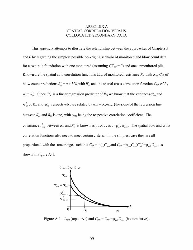
88

APPENDIX A

SPATIAL CORRELATION VERSUS COLLOCATED SECONDARY DATA

This appendix attempts to illustrate the relationship between the approaches of Chapters 5

and 6 by regarding the simplest possible co-kriging scenario of monitored and blow count data

for a two-pile foundation with one monitored (assuming CVεm = 0) and one unmonitored pile.

Known are the spatial auto correlation functions Cmm of monitored resistance Rm with Rm, Chh of

blow count predictions mR = a + bNh with mR and the spatial cross correlation function Cmh of Rm

with .mR Since mR is a linear regression predictor of Rm we know that the variances 2mm and

2hh of Rm and mR , respectively, are related by hh = mhmm (the slope of the regression line

between mR and Rm is one) with mh being the respective correlation coefficient. The

covariance 2mh between Rm and mR is known as mh mm hh =

2 2 .mh mm The spatial auto and cross

correlation functions also need to meet certain criteria. In the simplest case they are all

proportional with the same range, such that Chh = 2mh mmC and Cmh =

1/ 2 1/ 2mh mm hhC C = 2

mh mmC , as

shown in Figure A-1.

Figure A-1. Cmm (top curve) and Cmh = Chh =

2mh mmC (bottom curve).

h

Cmm, Chh, Cmh

0 ah Ds

2mm

212mm

2 2mh hh

212mh

89

With this, co-kriging of the monitored (= true because error assumed zero) resistance of the

unmonitored pile can be done. There are different types of co-kriging and the one with a single

bias condition as discusses in Isaaks and Srivastava (1989, Equation 17.15) is chosen here. The

ordinary co-kriging system results as

2 2 212 1 12

2 2 212 2

1

1

1 1 0 1

mm mh mm

mh hh mh

w

w

(A.1)

where 2

12mh is the covariance between Rm at the first (monitored) pile and mR at the second

(unmonitored) pile which are separated by a distance Ds. In analogy, 212mm is the covariance

between values of Rm at the two piles. From Figure A-1, it becomes clear that 212mh = 2

12.mh mm

While λ is the Lagrangian operator; w1 and w2 are the weights assigned to the monitored

resistance Rm1 of the first pile and of the predicted resistance 2mR of the second pile. They are

used in Equation A.2 to find an estimate 2mR of the monitored resistance Rm2 of the second pile as

2 1 1 2 2m m mR w R w R (A.2)

Note that w1 + w2 = 1 and that a single asterisk “*” denotes a regression estimate only from

collocated blow count information Nh, while double asterisks “**” denotes a co-kriging estimate

including information from monitored piles at other locations (here Rm1).

Equation 1 may be solved for w1, w2 and λ or, alternatively, using Cramer’s rule one can

directly express the ratio w1/w2 as

90

22212

212

212

22212

2212

212

2

22

212

212

2

1

011

1

1

011

1

1

mmmhmhmm

mmhhmhmh

mhmh

mmmm

hhmh

mhmm

w

w

(A.3)

With the relationships of Figure A-1 and by also introducing a spatial correlation coefficient

s= 2 212mm mm = 2 2

12mh mh as the auto correlation that persists over a lag distance Ds between

the piles, Equation A.3 simplifies to

2

2

2

1

11

1

mhs

mhs

w

w

(A.4)

which is shown by contour lines in Figure A-2. In Chapter 5, 2mR is disregarded in Equation A.2,

which is equivalent to using a large value of w1/w2 as it occurs in the yellow zone in Figure A-2.

This zone is located where s >> mh, i.e., where spatial correlation is dominant. In Chapter 6,

the opposite is the case and Rm1 is eliminated from Equation A.2. This corresponds to small

values of w1/w2 and the green zones in Figure A-2, i.e., where mh >> s and blow count

correlation dominates over spatial correlation. Interestingly from the data used in Chapter 6, it is

evident that the green zone is relevant (see arrow at mh ≈ 0.85) and neglecting Rm1 will not have

a large impact (w1 << w2; i.e., w1 would be close to zero anyway). Neglecting Rm1 is also

conservative as the estimation uncertainty should somewhat increase, but again not by much as

the weight of Rm1 in estimation would not be very significant. One can also see that for mh ≈

0.85, it does not make a large difference what particular s there is unless it is really close to 1,

which is irrelevant for practice. It is recalled that the error of the monitoring method was

neglected here; this error would always decrease s. Moreover, in many situations the values of

91

s are not even reliably known (e.g., unknown horizontal correlation length). Note that Figure

A-2 also indicates w2 >> w1 for both mh ≈ s ≈ 0. This is an artifact of the fact that the

regression estimate in the present form does not consider uncertainty due to limited data (from a

single unmonitored pile).

0 0.1 0.2 0.3 0.4 0.5 0.6 0.7 0.8 0.9 10

0.1

0.2

0.3

0.4

0.5

0.6

0.7

0.8

0.9

1

0.1

0.1

0.1

0.10.1

0.25

0.25

0.25

0.25

0.5

0.5

0.5

0.5

1

1

1

1

2

2

2

2

4

4

44

1010

10

mh

(-)

s (-)

Figure A-2. w1/w2 as a function of mh and s. Yellow zone is where spatial correlation is dominant (previous approach), green zone is where correlation between blow count and

monitored resistance is dominant. Green arrow indicates mh ≈ 0.85 from Caminida and Dixie data.

Overall, this is a very simple “elementary” example, but if the conclusion holds for a single

monitored and a single unmonitored pile, then it should also hold in some form for more

complex configurations.

resistance factors for 100% dynamic testing, with and

Documents