resonant circuits
TRANSCRIPT

1
Introduction To Resonant
Circuits

Group members
140080119002 Arjav Anil Patel
140080119003 Pruthil Bhatt
140080119001 Alok Sharma
140080119004 Vijay
2
3
Resonance In Electric Circuits
Any passive electric circuit will resonate if it has an inductorand capacitor.
Resonance is characterized by the input voltage and currentbeing in phase. The driving point impedance (or admittance) is completely real when this condition exists.
In this presentation we will consider (a) series resonance, and(b) parallel resonance.

4
Series Resonance
Consider the series RLC circuit shown below.
R L
C+
_ IV
V = VM ∠0
The input impedance is given by:
1( )Z R j wL
wC= + −
The magnitude of the circuit current is;
2 2
| |1
( )
mVI I
R wLwC
= =+ −
5
Series Resonance
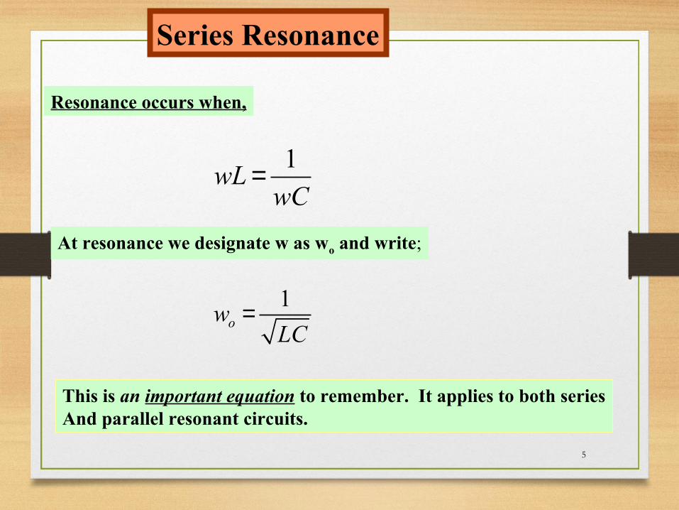
Resonance occurs when,
1wL
wC=
At resonance we designate w as wo and write;
1ow
LC=
This is an important equation to remember. It applies to both seriesAnd parallel resonant circuits.

6
Series Resonance
The magnitude of the current response for the series resonance circuitis as shown below.
mV
R
2mV
R
w
|I|
wow1 w2
Bandwidth:
BW = wBW = w2 – w1
Half power point
7
Series Resonance
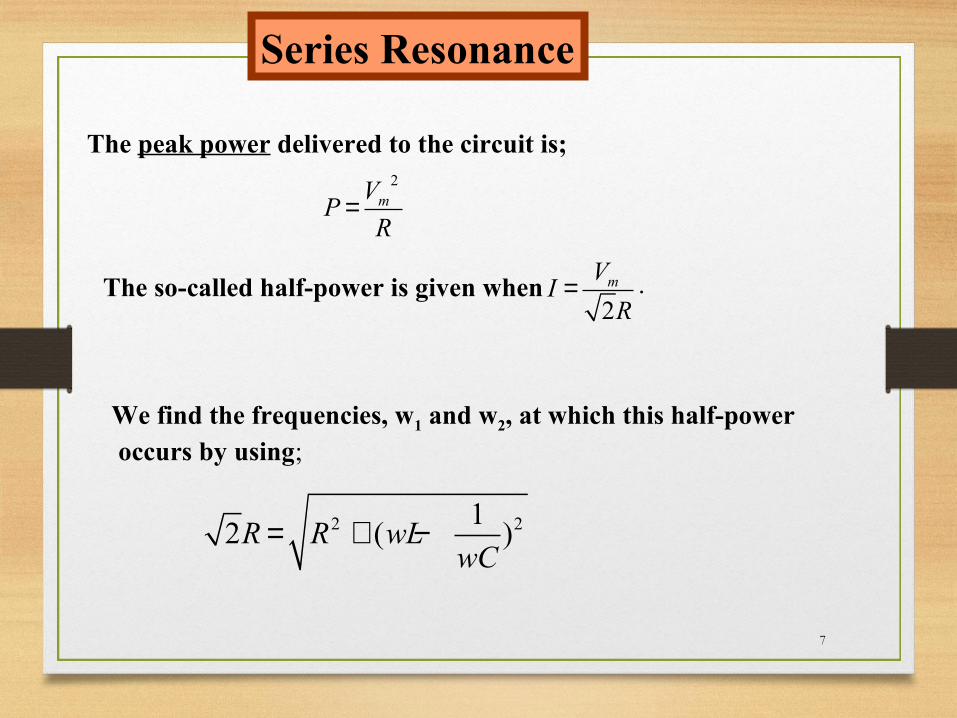
The peak power delivered to the circuit is;2
mVPR
=
The so-called half-power is given when2mVIR
= .
We find the frequencies, w1 and w2, at which this half-power occurs by using;
2 212 ( )R R wL
wC= + −

8
Series Resonance
After some insightful algebra one will find two frequencies at whichthe previous equation is satisfied, they are:
2
1
1
2 2
R Rw
L L LC = − + +
and
2
2
1
2 2
R Rw
L L LC = + +
The two half-power frequencies are related to the resonant frequency by
1 2ow w w=

9
Series Resonance
The bandwidth of the series resonant circuit is given by;
2 1b
RBW w w w
L= = − =
We define the Q (quality factor) of the circuit as;
1 1o
o
w L LQ
R w RC R C = = =
Using Q, we can write the bandwidth as;
owBWQ
=
These are all important relationships.

10
Series Resonance
An Observation:
If Q > 10, one can safely use the approximation;
1 22 2o o
BW BWw w and w w= − = +
These are useful approximations.

11
Series Resonance
An Observation:
By using Q = woL/R in the equations for w1and w2 we have;
2
2
1 11
2 2ow wQ Q
= + +
2
1
1 11
2 2ow wQ Q
− = + + and

12
Series Resonance
In order to get some feel for how the numerical value of Q influencesthe resonant and also get a better appreciation of the s-plane, we considerthe following example.
It is easy to show the following for the series RLC circuit.
2
1( ) 1
1( ) ( )
sI s LRV s Z s s sL LC
= =+ +
In the following example, three cases for the about transfer functionwill be considered. We will keep wo the same for all three cases.The numerator gain,k, will (a) first be set k to 2 for the three cases, then(b) the value of k will be set so that each response is 1 at resonance.

13
Series Resonance
An Example Illustrating Resonance:
The 3 transfer functions considered are:
Case 1:
Case 2:
Case 3:
2 2 400
ks
s s+ +
2 5 400
ks
s s+ +
2 10 400
ks
s s+ +
14
Series Resonance
An Example Illustrating Resonance:
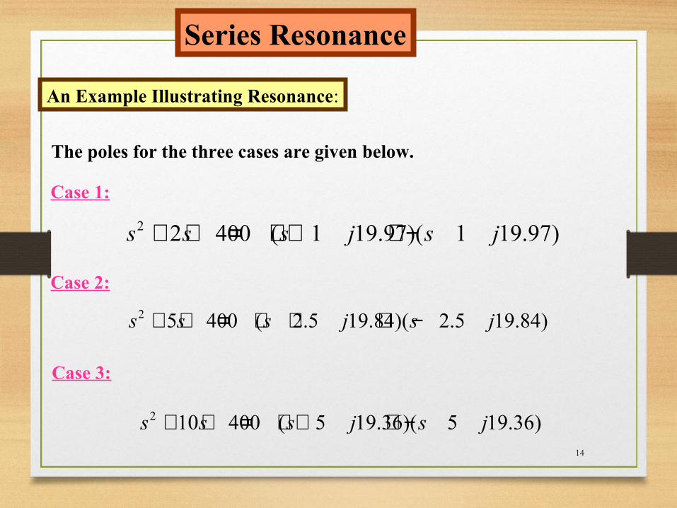
The poles for the three cases are given below.
Case 1:
Case 2:
Case 3:
2 2 400 ( 1 19.97)( 1 19.97)s s s j s j+ + = + + + −
2 5 400 ( 2.5 19.84)( 2.5 19.84)s s s j s j+ + = + + + −
2 10 400 ( 5 19.36)( 5 19.36)s s s j s j+ + = + + + −
15
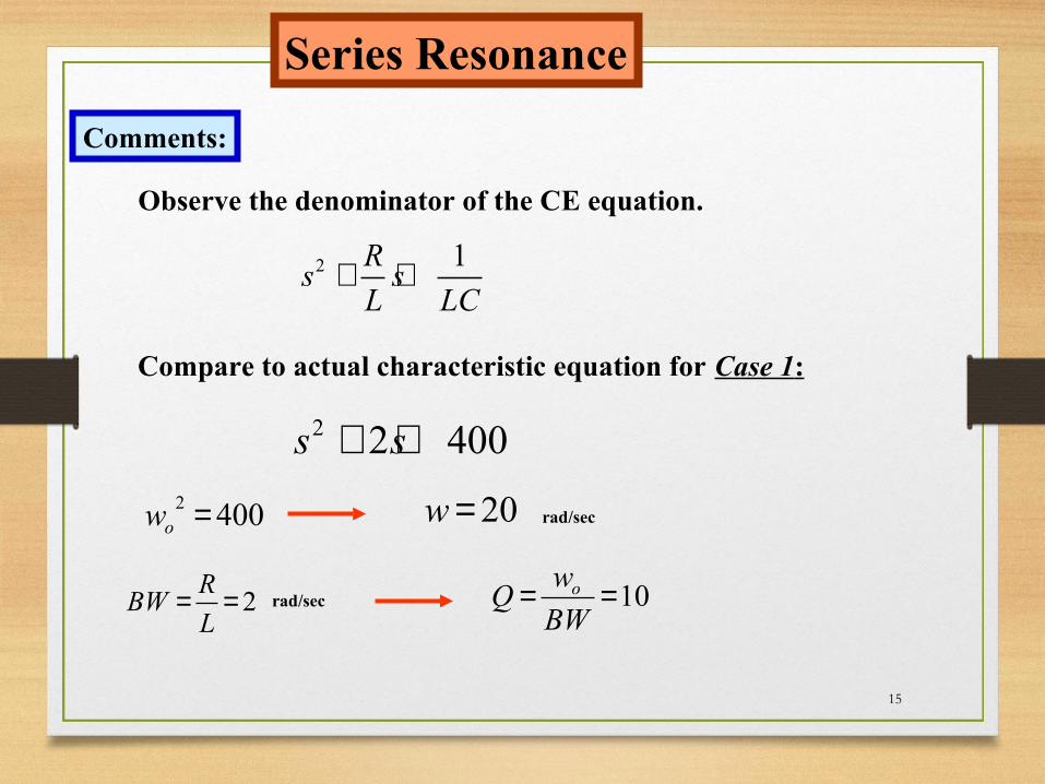
Series Resonance
Comments:
Observe the denominator of the CE equation.
2 1Rs s
L LC+ +
Compare to actual characteristic equation for Case 1:
2 2 400s s+ +2 400ow = 20w=
2R
BWL
= = 10owQBW
= =
rad/sec
rad/sec

16
Series Resonance
Poles and Zeros In the s-plane:
s-plane
jw axis
σ axis
00
20
-20xx
x x x
x
( 3) (2) (1)
( 3) (2) (1)
-5 -2.5 -1Note the location of the polesfor the three cases. Also notethere is a zero at the origin.
17
Series Resonance
Comments:
The frequency response starts at the origin in the s-plane.At the origin the transfer function is zero because there is azero at the origin.
As you get closer and closer to the complex pole, which has a j parts in the neighborhood of 20, the response startsto increase.
The response continues to increase until we reach w = 20.From there on the response decreases.
We should be able to reason through why the responsehas the above characteristics, using a graphical approach.

18
Series Resonance
Matlab Program For The Study:
% name of program is freqtest.m% written for 202 S2002, wlg%CASE ONE DATA:K = 2;num1 = [K 0];den1 = [1 2 400]; num2 = [K 0];den2 = [1 5 400]; num3 = [K 0];den3 = [1 10 400]; w = .1:.1:60;
gridH1 = bode(num1,den1,w);magH1=abs(H1); H2 = bode(num2,den2,w);magH2=abs(H2); H3 = bode(num3,den3,w);magH3=abs(H3); plot(w,magH1, w, magH2, w,magH3)gridxlabel('w(rad/sec)')ylabel('Amplitude')gtext('Q = 10, 4, 2')
19
0 10 20 30 40 50 600
0.1
0.2
0.3
0.4
0.5
0.6
0.7
0.8
0.9
1
w(rad/sec)
Am
plitu
de
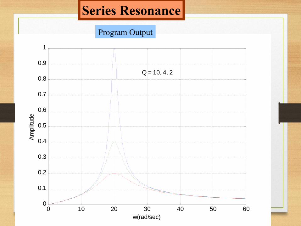
Q = 10, 4, 2
Series Resonance
Program Output

20
Series Resonance
Comments: cont.
From earlier work:2
1 2
1 1, 1
2 2ow w wQ Q
± = + + With Q = 10, this gives;
w1= 19.51 rad/sec, w2 = 20.51 rad/sec
Compare this to the approximation:
w1 = w0 – BW = 20 – 1 = 19 rad/sec, w2 = 21 rad/sec
So basically we can find all the series resonant parametersif we are given the numerical form of the CE of the transfer function.

21
Series Resonance
Next Case: Normalize all responses to 1 at wo
0 10 20 30 40 50 600
0.1
0.2
0.3
0.4
0.5
0.6
0.7
0.8
0.9
1
w(rad/sec)
Am
plitu
de
Q = 10, 4, 2

22
Series Resonance
Three dB Calculations:
Now we use the analytical expressions to calculate w1 and w2.
We will then compare these values to what we find from the Matlab simulation.
Using the following equations with Q = 2,
+
+= 1
2
1
2
1,
2
21 Qw
Qwww
oo
we find,w1 = 15.62 rad/sec
w2 = 21.62 rad/sec
23
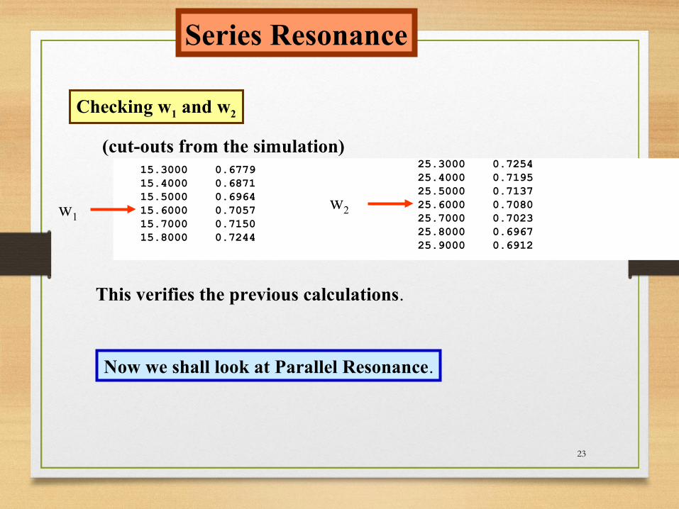
Series Resonance
Checking w1 and w2
15.3000 0.6779 15.4000 0.6871 15.5000 0.6964 15.6000 0.7057 15.7000 0.7150 15.8000 0.7244
w1
25.3000 0.7254 25.4000 0.7195 25.5000 0.7137 25.6000 0.7080 25.7000 0.7023 25.8000 0.6967 25.9000 0.6912
w2
This verifies the previous calculations.
Now we shall look at Parallel Resonance.
(cut-outs from the simulation)

24
++=
jwLjwC
RVI
11
++=
jwCjwLRIV
1
We notice the above equations are the same provided:
VI
RR
1
CL
If we make the inner-change,then one equation becomes the same as the other.
For such case, we say the one circuit is the dual of the other.
Series Resonance
Duality
If we make the inner-change,then one equation becomes the same as the other.
For such case, we say the one circuit is the dual of the other.
25
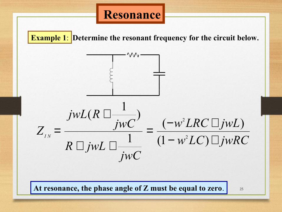
Resonance
Example 1: Determine the resonant frequency for the circuit below.
jwRCLCw
jwLLRCw
jwCjwLR
jwCRjwL
ZNI +−
+−=++
+=
)1(
)(1
)1
(
2
2
At resonance, the phase angle of Z must be equal to zero.

26
jwRCLCw
jwLLRCw
+−+−
)1(
)(2
2
ResonanceAnalysis
For zero phase;
LCw
wRC
LCRw
wL22 1()( −
=−
This gives;
12222 =− CRwLCw
or
)(
122CRLC
wo −=

27
Extension of Series Resonance
Peak Voltages and Resonance:
VS
R L
C
+
_ I
+ +
+
_ _
_
VR VL
VC
We know the following:
When w = wo =
1
LC, VS and I are in phase, the driving point impedance
is purely real and equal to R.
A plot of |I| shows that it is maximum at w = wo. We know the standardequations for series resonance applies: Q, wBW, etc.

28
Extension of Series Resonance
Reflection:
A question that arises is what is the nature of VR, VL, and VC? A little reflection shows that VR is a peak value at wo. But we are not sureabout the other two voltages. We know that at resonance they are equaland they have a magnitude of QxVS.
max 2
11
2ow wQ
= −
The above being true, we might ask, what is the frequency at which the voltage across the inductor is a maximum?
We answer this question by simulation
Irwin shows that the frequency at which the voltage across the capacitoris a maximum is given by;Irwin shows that the frequency at which the voltage across the capacitoris a maximum is given by;Irwin shows that the frequency at which the voltage across the capacitoris a maximum is given by;

29
Extension of Series Resonance
Series RLC Transfer Functions:
The following transfer functions apply to the series RLC circuit.
2
1( )
1( )C
S
V s LCRV s s sL LC
=+ +
2
2
( )1( )
L
S
V s sRV s s sL LC
=+ +
2
( )1( )
R
S
RsV s L
RV s s sL LC
=+ +

30
Extension of Series Resonance
Parameter Selection:
We select values of R, L. and C for this first case so that Q = 2 and wo = 2000 rad/sec. Appropriate values are; R = 50 ohms, L = .05 H, C = 5µF. The transfer functions become as follows:
6
2 6
4 10
1000 4 10C
S
V x
V s s x=
+ +
2
2 61000 4 10L
S
V s
V s s x=
+ +
2 6
1000
1000 4 10R
S
V s
V s s x=
+ +
31
Extension of Series Resonance
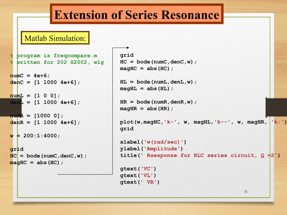
Matlab Simulation:
% program is freqcompare.m% written for 202 S2002, wlg numC = 4e+6;denC = [1 1000 4e+6]; numL = [1 0 0];denL = [1 1000 4e+6]; numR = [1000 0];denR = [1 1000 4e+6]; w = 200:1:4000; gridHC = bode(numC,denC,w);magHC = abs(HC);
gridHC = bode(numC,denC,w);magHC = abs(HC); HL = bode(numL,denL,w);magHL = abs(HL); HR = bode(numR,denR,w);magHR = abs(HR); plot(w,magHC,'k-', w, magHL,'k--', w, magHR, 'k:')grid xlabel('w(rad/sec)')ylabel('Amplitude')title(' Rsesponse for RLC series circuit, Q =2') gtext('VC')gtext('VL')gtext(' VR')

32
0 500 1000 1500 2000 2500 3000 3500 40000
0.5
1
1.5
2
2.5
w(rad/sec)
Am
plitu
de Rsesponse for RLC series circuit, Q =2
VC VL
VR
Exnsion of Series Resonance
Simulation Results
Q = 2

33
Exnsion of Series Resonance
Analysis of the problem:
VS
R=50 Ω L=5 mH
C=5 µF+
_ I
+ +
+
_ _
_
VR VL
VC
Given the previous circuit. Find Q, w0, wmax, |Vc| at wo, and |Vc| at wmax
Solution: sec/20001051050
1162
radxxxLC
wO
===−−
250
105102 23
===−xxx
R
LwQ O

34
Exnsion of Series Resonance
Problem Solution:
oOMAXw
Qww 9354.0
2
11
2=−=
)(212|||| peakvoltsxVQwatVSOR
===
( ))066.2968.0
2
4
11
||||
2
peakvolts
Q
VQxwatV S
MAXC==
−=
Now check the computer printout.

35
Exnsion of Series Resonance
Problem Solution (Simulation):
1.0e+003 *
1.8600000 0.002065141 1.8620000 0.002065292 1.8640000 0.002065411 1.8660000 0.002065501 1.8680000 0.002065560 1.8700000 0.002065588 1.8720000 0.002065585 1.8740000 0.002065552 1.8760000 0.002065487 1.8780000 0.002065392 1.8800000 0.002065265 1.8820000 0.002065107 1.8840000 0.002064917
Maximum

36
Extension of Series Resonance
Simulation Results:
0 500 1000 1500 2000 2500 3000 3500 40000
2
4
6
8
10
12
w(rad/sec)
Am
plitu
de Rsesponse for RLC series circuit, Q =10
VC VL
VR
Q=10
37
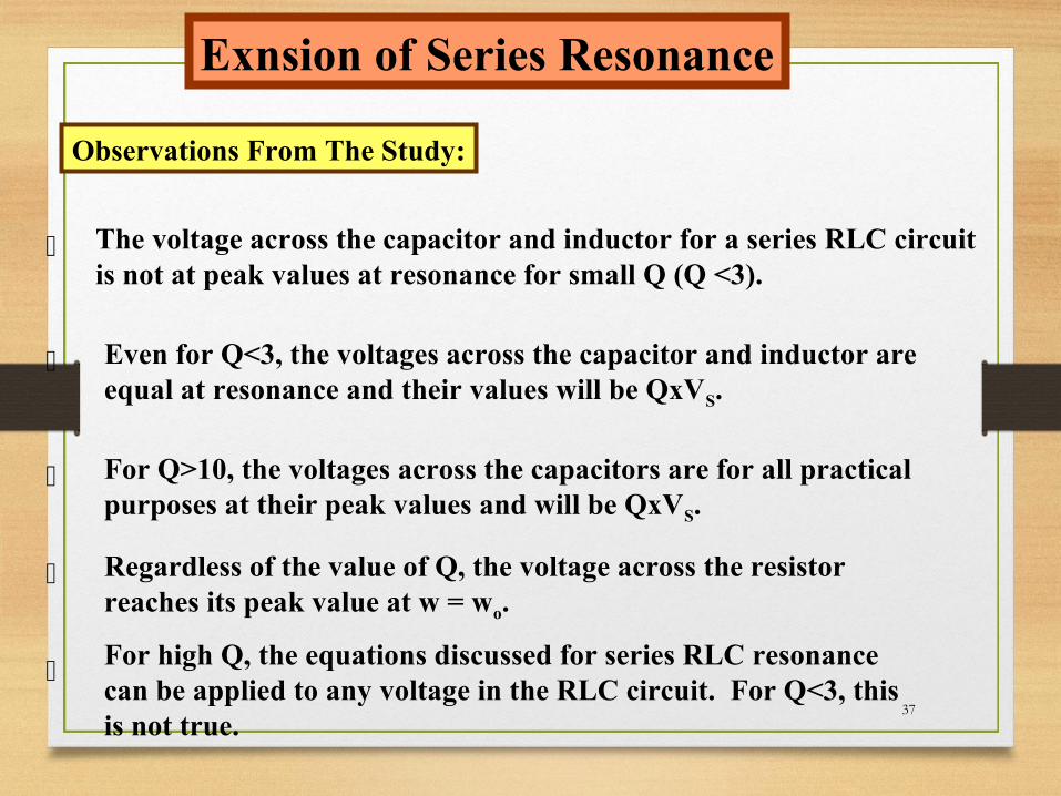
Exnsion of Series Resonance
Observations From The Study:
The voltage across the capacitor and inductor for a series RLC circuitis not at peak values at resonance for small Q (Q <3).
Even for Q<3, the voltages across the capacitor and inductor areequal at resonance and their values will be QxVS.
For Q>10, the voltages across the capacitors are for all practical purposes at their peak values and will be QxVS.
Regardless of the value of Q, the voltage across the resistor reaches its peak value at w = wo.
For high Q, the equations discussed for series RLC resonancecan be applied to any voltage in the RLC circuit. For Q<3, thisis not true.

38
Extension of Resonant Circuits
Given the following circuit:
I
+
_
+
_
VC
R
L
We want to find the frequency, wr, at which the transfer functionfor V/I will resonate.
The transfer function will exhibit resonance when the phase anglebetween V and I are zero.

39
Extension of Resonant Circuits
The desired transfer functions is;
(1/ )( )
1/
V sC R sL
I R sL sC
+=+ +
This equation can be simplified to;
2 1
V R sL
I LCs RCs
+=+ +
With s jw
2(1 )
V R jwL
I w LC jwR
+=− +
40
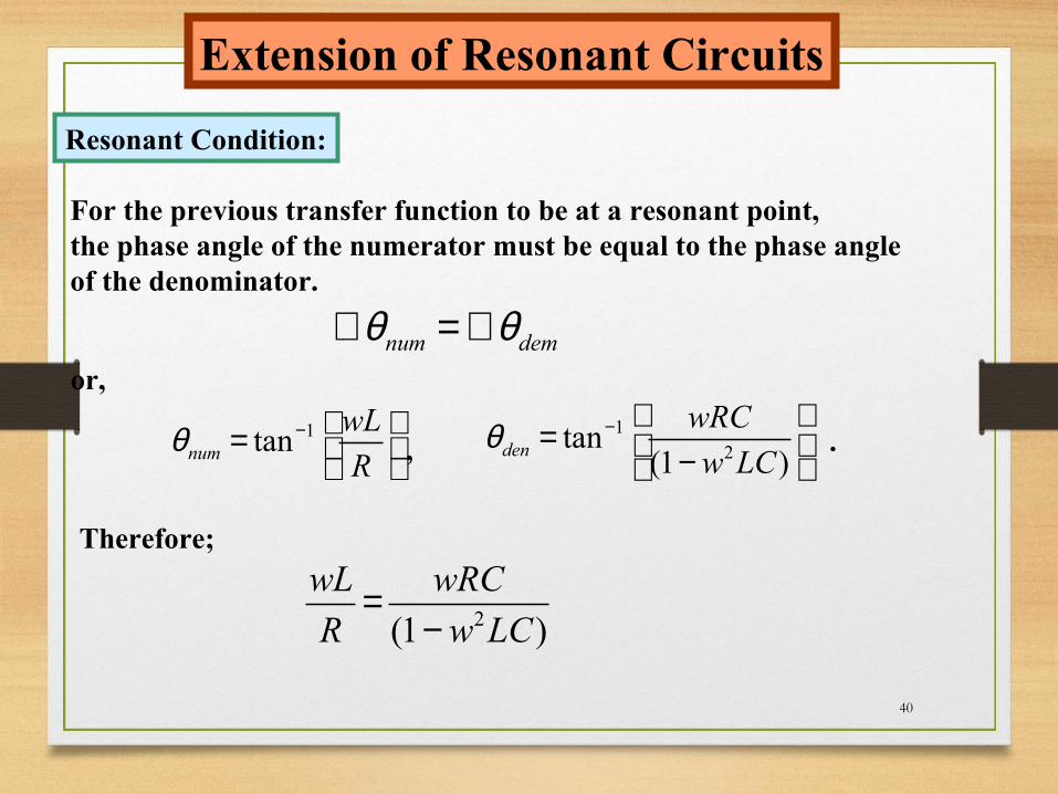
Extension of Resonant Circuits
Resonant Condition:
For the previous transfer function to be at a resonant point,the phase angle of the numerator must be equal to the phase angleof the denominator.
num demθ θ∠ = ∠
1tannum
wL
Rθ − =
or,
12
tan(1 )den
wRC
w LCθ −
= − , .
Therefore;
2(1 )
wL wRC
R w LC=
−
41
Extension of Resonant Circuits
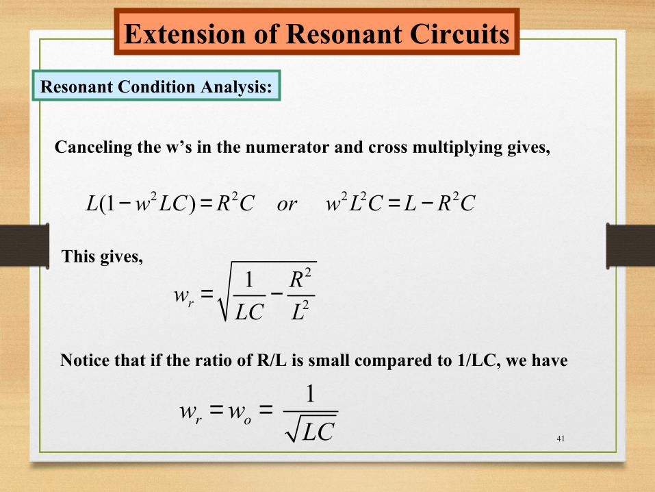
Resonant Condition Analysis:
Canceling the w’s in the numerator and cross multiplying gives,
2 2 2 2 2(1 )L w LC R C or w L C L R C− = = −
This gives,2
2
1r
Rw
LC L= −
Notice that if the ratio of R/L is small compared to 1/LC, we have
1r ow w
LC= =

42
Extension of Resonant Circuits
Resonant Condition Analysis:
What is the significance of wr and wo in the previous two equations?Clearly wr is a lower frequency of the two. To answer this question, considerthe following example.
Given the following circuit with the indicated parameters. Write a Matlab program that will determine the frequency response of the transfer function of the voltage to the current as indicated.
I
+
_
+
_
VC
R
L
43
Extension of Resonant Circuits
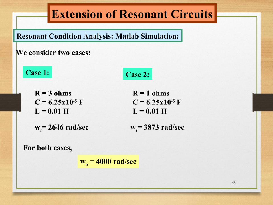
Resonant Condition Analysis: Matlab Simulation:
We consider two cases:
Case 1:
R = 3 ohmsC = 6.25x10⁻⁵ FL = 0.01 H
Case 2:
R = 1 ohmsC = 6.25x10⁻⁵ FL = 0.01 H
wr= 2646 rad/sec wr= 3873 rad/sec
For both cases,
wo = 4000 rad/sec
44
Extension of Resonant Circuits
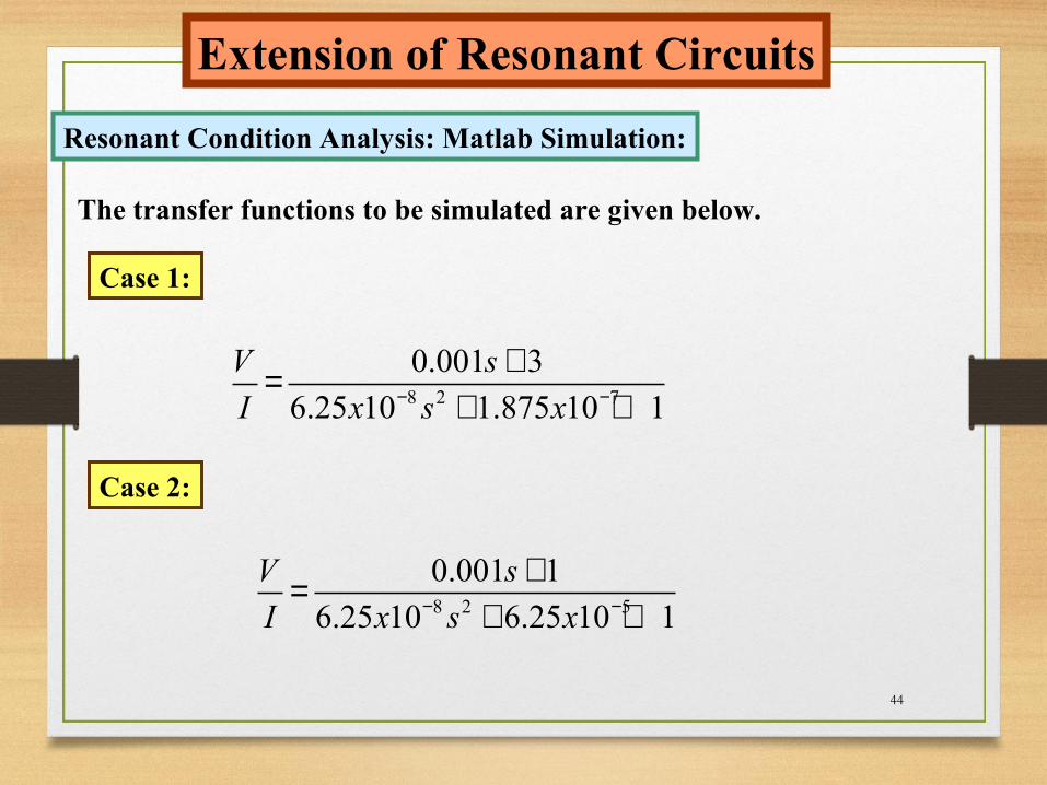
Resonant Condition Analysis: Matlab Simulation:
The transfer functions to be simulated are given below.
8 2 7
0.001 3
6.25 10 1.875 10 1
V s
I x s x− −
+=+ +
Case 1:
Case 2:
8 2 5
0.001 1
6.25 10 6.25 10 1
V s
I x s x− −
+=+ +
45
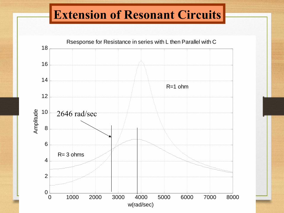
Extension of Resonant Circuits
0 1000 2000 3000 4000 5000 6000 7000 80000
2
4
6
8
10
12
14
16
18
w(rad/sec)
Am
plitu
de Rsesponse for Resistance in series with L then Parallel with C
R= 3 ohms
R=1 ohm
2646 rad/sec

46
Extension of Resonant Circuits
What can be learned from this example?
wr does not seem to have much meaning in this problem.What is wr if R = 3.99 ohms?
Just because a circuit is operated at the resonant frequencydoes not mean it will have a peak in the response at the frequency.
For circuits that are fairly complicated and can resonant,It is probably easier to use a simulation program similar toMatlab to find out what is going on in the circuit.

47
End of Lesson
Basic Laws of Circuits
Resonant Circuits
Circuits