resource abundance and economic growth in china

Resource Abundance and Economic Growth in China∗

Rui Fan † Ying Fang ‡ Sung Y. Park §

Abstract

This paper studies the resource curse phenomenon in China. The “resource curse” is an impor-tant claim that the resource-abundant economies grow at a slower pace than the resource-scarceeconomies do. There are many recent studies that analyze the resource curse phenomenon theoreti-cally and empirically. However, few papers analyze which socio-economic variables determine theresource curse. This paper is different from the previous studies in three aspects: (i) The city-leveldata is used; (ii) Using the functional coefficient regression model we can take care of city-specificheterogeneity and, at the same time, analyze the transmission mechanism of the curse of recourses;(iii) We construct a variable to estimate the effect of the diffusion processes of the natural resourcesamong cities in the same province. Our empirical results show that there is no evidence to supportthe statement of resource curse in China. On the other hand, the level of natural resources in a cityimposes a significant positive diffusion effect on the economic growth of neighbor city within thesame province.

JEL code: O13; O18Key words: Resource curse; Diffusion effects; Transmission channels; Functional coefficientModel;

∗Previous title of this paper was “Diffusion Effects or Curse of Resources? An Evidence from China”. Theauthors would like to thank Zhigang Li, Yiu Por Che, Chun-Chung Au, Ji Kan, and the participants in conferencesand seminar in Young Economist Society (YES), Xiamen University, April 3-4, 2010, Brownbag Seminar at WISE,Xiamen University, May 15, 2010, and Chinese Economists Society (CES), Xiamen University, June 19-21, 2010 formany pertinent comments and discussions. However, we retain the responsibility for any remaining errors.

†The Wang Yanan Institute for Studies in Economics, Xiamen University, Xiamen, Fujian 361005, China.‡The Wang Yanan Institute for Studies in Economics, MOE Key Laborary of Econometrics, and Fujian Key Lab-

oratory of Statistical Sciences, Xiamen University, Xiamen, Fujian 361005, China.§Corresponding Author: Department of Economics, Chinese University of Hong Kong, Shatin, NT, Hong Kong,

China. Tel: +852-2609-8001, Fax: +852-2603-5805. Email: [email protected].

1

brought to you by COREView metadata, citation and similar papers at core.ac.uk

provided by Xiamen University Institutional Repository

https://core.ac.uk/display/41362935?utm_source=pdf&utm_medium=banner&utm_campaign=pdf-decoration-v1

1 Introduction

Many recent studies try to answer a fundamental question whether natural resource is an important

engine of economic growth [Leite and Weidmann, 1999; Papyrakis and Gerlagh, 2004; Rodriguez

and Sachs, 1999; Sachs and Warner, 1995, 1997, 1999 among many others]. Their common finding

is that natural resource-abundant countries have slower economic growth rates than those of nat-

ural resource-scarce economies. This phenomenon is referred to the term “resource curse” in the

literature, and it is quite widely accepted. However, it is hard to believe that the natural abundance

has the direct effect on the low economic growth rates. Therefore, some recent studies analyze

which socio-economic variables do generate the negative correlation between economic growth

and natural resource abundance [Angrist and Kugler, 2008; Auty, 1990; Gelb, 1988; Gylfason,

2000; Kronenberg, 2004; Papyrakis and Gerlagh, 2004; Sachs and Warner, 1995 among many oth-

ers]. For examples, Gelb (1988) and Auty (1990) argue that the resource rich countries are likely to

pay more attention to the rent-seeking behavior rather than other productive activities. Following

Matsuyama’s (1992) approach, Sachs and Warner (2001) find that resource-abundant economies

put more weights on the natural resource goods rather than manufacturing goods. Eventually, this

behavior could keep their economies staying at the low level of economic growth. Gylfason (2000)

points out that the level of education is also important factor for the resource curse phenomenon.

Kronenber (2004) finds that corruption is the major determinant for the curse of natural resources.

Even though some studies analyze the relationship between economic growth and natural re-

sources and its transmission channels, few consider this problem in a country level, say, many

different regions within a country. To our knowledge, Papyrakis and Gerlagh (2007) is the first

study analyzing the “resource curse” within a country. They investigate 49 U.S. states and find

evidences for the resource curse in U.S. In particular, they find that resource abundance decreases

investment, schooling, openness and R&D expenditure and increases corruption. In the similar

2

way, using a panel data, Zhang, Xing, Fan and Luo (2008) study the relationship between resource

abundance and regional development in China. They find that Chinese provinces with abundant

resources perform worse than their resource-poor counterparts in terms of per capita consumption

growth when they consider provinces located inland of China. When they use the whole sample

that covers most provinces in China, they cannot support the resource curse in China. Fang, Qi and

Zhao (2009) explicitly considers the problem of the “curse of resources” in China. They find that

there are no relationship between regional income growth and resource abundance.

Even though some studies, for examples, Papyrakis and Gerlagh (2004, 2007) and Fang, Qi

and Zhao (2009), consider the role of the transmission mechanism empirically, their approach has

some crucial drawbacks. In order to estimate the effect of transmission mechanism they consider

two different regression equations. From the estimates of these two independent regression models

they calculate the effect of transmission mechanism. However, since one cannot construct standard

errors of these estimates in an usual way, a classical t-test cannot be performed to check whether

considered transmission channels are important for the relationship between resource abundance

and regional economic growth.

This paper is different from the previous researches in three aspects: (i) Instead of using the

province-level data we collect the city-level data and analyze the relationship between resource

abundance and regional economic growth. This could provide more interesting and specific fea-

tures of the relationship; (ii) We use a functional coefficient regression model which turns out

quite useful and flexible in our analysis. Using the functional coefficient regression model we can

take care of heterogeneity of each city and specify the transmission mechanism between natural

resources and the economic growth simultaneously. Thus our model can give more direct inter-

pretation for the role of transmission channels; (iii) Due to China’s special governance policy, the

diffusion effect of natural resources among cities is of importance and interest for economic and

political policies in a particular province. We explicitly construct a variable which represents the

3

diffusion process from resource-rich cities to resource-scarce cities using the difference of natural

resource and physical distance between two cities.

Our results show that there is no supportive evidence to the “resource curse” phenomenon in

city level of China over the period 1997-2005 for the 95 cities. By applying the functional coeffi-

cient regression model, we observe the estimated regression coefficients of natural abundance on

economic growth of regional economy are significantly positive when the relative scale of manu-

facturing industry, innovation (R&D), institutional quality and openness are considered as trans-

mission channels, respectively. Especially, through the channel of manufacture, we find an inverted

U-shape relationship between natural resource and economic growth which indicates that one unit

of natural resource affects the growth of regional economy differently depending on levels of indus-

trialization. We believe that this result is useful for Chinese policy makers to establish appropriate

economic and political policies based on the fact of different degrees of industrialization between

inland and coastal regions in China. Moreover, our empirical results for the diffusion effect show

that the abundance of natural resources encourages not only the local economic development but

also boosts the growth of economy in other cities in the same province, which is consistent with

the big-push theory explored by Rosenstein-Rodan (1943). This diffusion phenomenon is signifi-

cant through the economic transmission channels such as manufacture, innovation, human capital

investment and openness.

The next section provides the model that explains the relationship between resource abundance

and economic growth and its estimation method. Section 3 offers our empirical results which verify

our main proposition that natural resource abundance is an engine for economic development at a

city level in China. Section 3 also focuses on transmission channels of natural resources (manufac-

turing industry, innovation, human capital investment, institutional quality and openness). Finally,

conclusions are followed in Section 4.

4

2 The Model

2.1 Basic Model

Most empirical studies for analyzing the resource curse consider the linear empirical growth re-

gression model. We start with the basic linear regression model specification:

Gi = α0 + α1 ln Y1990,i + α2miningi + z′iξ + ui, (1)

where Gi denotes the growth rate of income per capita of a city i from 1997 (initial period) to 2005,

that is, Gi = ln(Y2005,i/Y1997,i), Y1990,i is the initial income of a city i in 1990, miningi is the average

fraction of workers who are in mining industries at a city i from 1997 to 2005, zi and ξ are the

vector of other demographic variables and its corresponding parameter vector, respectively, and ui

denotes the disturbance term.

Although the regression model (1) is frequently used and useful to analyze the resource curse

phenomenon, it does not tell us which factors are important to explain the partial effect of miningi

on Gi, i.e., transmission channels that links the line between economic growth and natural resource

abundance. Papyrakis and Gerlagh (2004, 2007) propose a simple method to answer this question.

They consider an additional regression equation given by

z1,i = β0 + β1 ln Y1990,i + β2miningi + z′i ξ + µi, (2)

where z1,i is a variable in zi, which is believed to be a link variable between the income growth

rate and resource abundance, zi denotes all variables in zi except for z1,i, ξ is ξ excluding ξ1 and µi

denotes a random disturbance term. One can substitute z1,i of (2) into (1) and obtain

Gi = (α0 + ξ1β0) + (α1 + ξ1β1) ln Y1990,i + (α2 + ξ1β2)miningi + z′i(α2 + ξ1ξ) + εi, (3)

where εi = ξ1µi + ui. In equation (3), α2 is the direct effect of natural resources on growth, ξ1β2 is

the indirect effect of natural resources on growth through z1,i. In this way, Papyrakis and Gerlagh

5

(2004) take care of the ‘indirect effect’ of the resource abundance on growth rate based on (3).

However, it is clear that parameters in (3) cannot be identified. Thus in order to specify the direct

and indirect effects they need to estimate (1) and (2) at the same time. One major problem of the

above method is that one cannot obtain the standard error of the indirect effect. Thus one cannot

perform a simple inference procedure whether the indirect effect is statistically significant. And,

moreover, the suggested method is quite ad-hoc to study the transmission channels.

It is worth noting that z1,i in (2) is determined by the parameters, β0, β1 and β2 conditional on

the covariates. Thus the above (3) can be written by a general form

Gi = φ0(z1,i) + φ1(z1,i) ln Y1990,i + φ2(z1,i)miningi + z′i ξ(z1,i) + εi, (4)

where φk(·), k = 0, 1, 2 and ξ(·) are functional coefficients. The model (4) is known as the func-

tional coefficient regression model in the literature. This model has at least two advantages for

studying the relationship between natural resources and economic development: (i) The functional

coefficient model explicitly incorporates the indirect effect in the model, for example, φ2(z1,i) rep-

resents the causal relationship between natural resources and the grow rate of income is affected

by some index variable z1,i. Thus estimation procedure for two regression models (1) and (2) is

not needed; (ii) As we mentioned before, the linear regression model (1) is frequently used in

the empirical growth literature. However, such linear specification is due to the assumption of

identical aggregate production function of each country (Mankiw, Romer and Weil (1992)). This

homogeneity assumption is hard to be implemented in the real world. However, the coefficients in

(4) are different in each country depending on the index variable z1,i. Thus it can take care of the

city-specific heterogeneity within the model (Durlauf, Kourtellos and Minkin (2001)). With the

above reasons we use (4) to analyze the relationship between natural resource abundance and re-

gional economic growth with transmission channels. However, one drawback of the above model

is the non-identification problem for the direct and indirect effects separately. This can be taken

care of, if possible, assuming a flexible parametric function. However, in this paper, we do not

6

consider this functional specifications to identify the direct and indirect effects, but we estimate

φi(z1,i), i = 0, 1, 2 using non-parametric estimation methods.

2.2 Diffusion effect

Since the local government in a province has an independent right for the distribution of economic

resources including natural resources the interacting behavior among cities in the same province

could provide useful information for making policy decisions. Thus it is of interest to see how the

economic growth rate of a city is affected by the resource abundance of her neighborhood. For the

spill-over effect, Fang, Qi and Zhao (2009) consider the following linear regression model

Gi = α0 + α1 ln Y1990,i + α2miningi + α3Di + z′iξ + ui, (5)

where Di is a dummy variable, i.e., Di = 1 if city i locates in the province that contains top 10

resource abundant cities out of 96 cities. They argue that there exists a spill-over effect if α3

is significant. However, it is not quite clear whether α3 represents the spill-over effect since Di is

nothing but the province dummy variable. Positive significance of α3 only tells us that the province

in which are resource abundant cities yields higher regional income growth. Thus we can say that

Di may not represent diffusion processes among cities in the same province.

For the diffusion effect we may want to check whether “because resource-rich cities in my

province are my neighbors, my city is better-off” is true. In order to define the variable that

measures the diffusion of natural resource we need to consider the following two things. At first,

we need to define the “direction” of the diffusion. The diffusion effect between two cities can be

categorized by uni-directional or bi-directional diffusion effect. For simplicity, we assume that

only resource-rich cities influence resource-poor cities. However, when two cities in the same

neighborhood have similar amount of natural resource, the diffusion process can be bi-directional

one. Secondly, we also need to define the “neighborhood” carefully. Denote cmk by a m-th city

7

located in k-th province, m = 1, 2, · · · , Mk and k = 1, 2, · · · ,K. Since provinces are entitled with

relatively independent distribution rights in natural resource, we can set the maximum boundary

of neighborhood of m-th city in k-th province by the physical boundary of k-th province, say,

Pk. For each city m in province k, cmk, we can construct a ball, Bmk ∈ Pk, which represents the

neighborhood of a city cmk. Then for each province k we can define a variable that represents the

spill-over phenomenon from city c jk to cmk for j , m

UUm ≡ Umk =∑

j∈{1,2,··· ,Mk}\{m}

[ω j(Rk

j − Rkm)1{Rk

j>Rkm} | c jk ∈ Bmk ⊆ Pk

], (6)

where ω j is a distance-based weight given by ω j = (1/distm j)/(∑

j(1/distm j)) in which distm j de-

notes a distance between cities m and j based on their longitudes and latitudes, Rkj denotes natural

resource abundance at city j in province k, and 1{·} is the indicate function. The diffusion vari-

able Umk is nothing but a (asymmetrically) weighted average of difference in natural resource

abundance between two cities with pre-specified uni-direction. It can be easily extended to bi-

directional weighted function by substituting 1{Rkj>Rk

m} by 1{Rkj−Rk

m>κ} for some constant κ. Note that

the mixed spatial autoregressive model can be also considered for the above model specification.

The weight matrix of the spatial autoregressive model can be specified using rank information of

natural resource abundance. However, it is relatively hard to estimate the mixed spatial autoregres-

sive model due to some computational burdens and endogeneity problem. Thus we use UUm to

estimate the diffusion effect in this paper.

2.3 Model Estimation

For our empirical analysis we consider the functional coefficient model (4) with an additional

covariate Umk in (6):

Gi = φ0(z1,i) + φ1(z1,i) ln Y1990,i + φ2(z1,i)miningi + φ3(z1,i)UUi + z′i ξ(z1,i) + εi. (7)

8

For the estimation methodology, as suggested by Fan and Gijbels (1996), one can estimate the

coefficient functions {φ j(·)} using the local linear regression method from observation {Zi,Xi,Yi},where Xi = (Xi1, · · · , Xip)′. Assuming φ j(·) has a continuous second derivative, φ j(·) can be ap-

proximated locally at z0 by a linear function γ j(z) ≈ φ j + b j(z − z0). The local linear estimator,

{(φ j, b j)}, minimizes the sum of weighted squares

n∑

i=1

Yi −p∑

j=1

{φ j + b j(Zi − z0)}Xi j

2

Kh(Zi − z0),

where Kh(·) = h−1K(·/h), K(·) denotes a kernel function and h > 0 is a bandwidth. Then the local

linear estimator at z0 can be easily calculated by

φ j(z0) =

K∑

k=1

Kn, j(Zk − z0,Xk)Yk,

where

Kn, j(z, x) = e′j,2p(X′WX)−1(

xzx

)Kh(z),

e j,2p is the 2p × 1 unit vector with 1 at j-th element, X denotes an n × 2p matrix with its i-th

row (X′i ,X′i(Zi − z0)) and W = diag{Kh(Z1 − z0), · · · ,Kh(Zn − z0)}. For the selection of band-

width h, there are some techniques in the non-parametric statistics literature, for example, Rup-

pert, Sheather and Wand (1995) and Fan and Gijbels (1996) among others. In this paper we use

a boundary kernel suggested by Dong and Jiang (2000) to take care of the boudary problem in

non-parametric estimation procedure. Their kernel function has three different forms depending

on the data. In the central region of the data the kernel function is given by the Epanechnikov

kernel, K(z) = 0.75(1 − z2)I(|z| ≤ 1). For both tail parts, boundary kernels are considered to deal

with the boundary problem.

One crucial drawback of the above method is that all slope functional coefficients have the

same degree of smoothness since they depend only on one bandwidth parameter, h. Thus if {φ j(·)}have difference degrees of smoothness, the above estimators are sub-optimal. In reality, it is always

9

possible that each φ j(·) may have different degree of smoothness. In order to deal with this prob-

lem, we adopt a two-step estimation method proposed by Fan and Zhang (1999). Without loss of

generality, let us consider the estimation for the φp(·) of φ j(·), j = 1, 2, · · · , p. In the first step, the

initial (first) estimates of {φ j(·)}, j = 1, 2, · · · , p − 1 are estimated using small enough bandwidth

h, which ensures the bias of the estimator is small. From these estimates one can obtain the partial

residual,

εi,−p = Gi − φ1(z)Xi1 − · · · − φp−1(z)Xi,p−1.

In the second step one solves the following local cubic problem

minap,bp,cp,dp

n∑

i=1

[εi,−p − (ap + bp(Zi − z0) + cp(Zi − z0)2 + dp(Zi − z0)3)Xip

]2Kh2(Zi − z0),

where h2 denotes the second step bandwidth. In the above estimation procedure the choice of the

first bandwidth does not affect the final result substantially. Fan and Zhang (1999) show that the

two-step estimator has the optimal rate of convergence for the asymptotic mean squared errors,

and it always yields better performance than the classical local least square estimator does. In this

paper we use the least squares cross-validation method to choose the optimal bandwidth, h2, in the

second step estimation procedure [Hardle and Marror (1985) and Hardle, Hall and Marror (1992)].

3 Empirical Results

3.1 Data

We employ the data from volumes of Chinese Statistical Yearbooks and World Bank Report (2006).

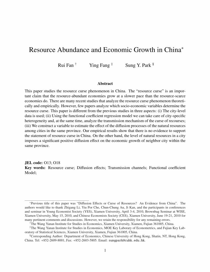
The GDP growth rates and other variables for 95 main cities in China are constructed using the

data from 1997 to 2005. Note that the GDP of these 95 cities contributed for 47.7% of the national

GDP in 1995. Figure 1 plots locations and resource abundance of all cities.

[Figure 1]

10

We consider five transmission variables: (i) manufacture: an average ratio of value of the manufac-

turing industry production to the local GDP from 1997 to 2005; (ii) R&D: the ratio of R&D related

workers to the local population; (iii) teacher (human capital investment): an average percentage of

the number of teachers from primary schools, middle schools and universities in the local popula-

tion; (iv) court (institutional quality): confidence in court; (v) FDI (openness): the ratio of usage

of foreign direct investment (FDI) to the local GDP.1

Since the appropriate proxy for the abundance of natural resources is essential to the analysis of

this paper, it is necessary to discuss how we obtain sufficient information about natural resources

on the city level in China. Conventionally, many previous empirical studies provide three options

for the measurement of natural resources: natural resource production, natural resource reserves

and exports of primary products. However, these options are highly restricted for our study since

they are incomplete and limited to access. It is worth stressing that endogeneity is a potential prob-

lem in all these options. For example, Stijns (2005) argues that it is possible that reserves data for

natural resources depend on economic growth because rich countries are able to investigate their

ground longer and in more efficient ways. This paper does not attempt to discuss this possible

problem. Alternatively, we use the fraction of mining workers to the total local population to cap-

ture resource abundance. This measurement includes nearly all natural resource industries such as

oil, coal, and nonferrous metal. Given the availability of the data, we believe that our chosen proxy

represents resource abundance as close as possible.

3.2 Empirical Results

In case of the provincial level data, Zhang et.al. (2008) show that per capita consumption growth

rates of resource-abundant provinces are lower than those of resource-poor counterparts. Since the

1Usually, openness is measured by the ratio of export and import to GDP. However, due to the limitation of citylevel data, we use the ratio of usage of FDI to the local GDP to measure “openness”.

11

sample size of provincial data is relatively small they used a pooled regression model to analyze

the resource curse in China. In this paper we consider city-level data to study the curse of resource

phenomenon in China. Due to the relatively large sample size of the city level data, our study could

provide more trustable results for the curse of resources phenomenon in China. Moreover, we also

study how the resource abundance of a city affects its neighbor cities’ regional economic growth

through different transmission channels.

At first, we start with simple linear regression models to check the existence of the resource

curse and diffusion effects. We consider six regression models that are special cases of the follow-

ing model

Gi = α0 + α1Miningi + α2Dlandlocki + α3Dspeciali + α4Xinteri + α5 log Y1990,i + α6UUi + εi, (8)

where Dlandlocki is a dummy variable for a coastal city and Dspeciali denotes a dummy variable

representing a municipality directly under the government or a special economic zone or a capital

of the province, Xinteri denotes Dlandlocki × log Y1990,i which also used in Sachs and Warner

(1995), and log Y1990,i is the logarithm of GDP per capita in 1990.2 The estimation results for six

models are reported in Table 1.

[Table 1]

From Table 1 it is clear that estimated coefficients of Miningi are positive, but they are insignificant

except for M6 that includes natural resource variable, Miningi, and spatial diffusion variable, UUi,

at the same time. It turns out that Miningi and UUi are both positive and significant. These results

support that resource curse phenomenon does not exist, and a positive diffusion effect among cities

exists in China. However, the above linear regression models cannot shed some lights on transmis-

sion channels that link the line between economic growth and natural resources. In this paper, we2Since China’s economic system reform took off in nearly all big cities in 1990, we set 1990 as the initial GDP per

capita year.

12

analyze that natural resources are associated with not only economic growth but also some other

important economic channels such as manufacturing activities, human capital and openness of the

economy. Moreover, the above models impose quite strong homogeneity assumption, for example,

each city has the identical production technology. This assumption obviously weakens the validity

of the empirical results since it is hard to believe each city has the same production function.

We now turn to the functional coefficient model discussed in Section 2:

Gi = φ0(z1,i) + φ1(z1,i) ln Y1990,i + φ2(z1,i)Miningi + φ3(z1,i)UUi + z′i ξ(z1,i) + εi, (9)

where z1,i is a transmission variable that is commonly used in the literature such as manufacturing

activities, R&D, human capital investment, institutional quality and openness (Gylfason, 2001;

Matsuyama, 1992; Papyrakis and Gerlagh, 2004, 2007; Sachs and Warner, 1999, 2001). Since

dummy variables in (8) are insignificant we do not include dummy variables in (9).

We estimate equation (9) with various transmission channels that affect the relationship be-

tween resource abundance and the growth of regional economy. As we mentioned before, co-

efficients of all the variables in our model are varying based on different values of a particular

transmission channel, which is different from the classical regression analysis. These varying co-

efficient estimates help us determine which channels are crucial in the relationship of resource

and economic growth. More interestingly, it also tells us precisely that how much influence the

channels have on the association of natural resource and local economy.

[Figure 2]

Figure 2 shows the estimation results when the relative scale of manufacturing industry is se-

lected as the transmission channel. It is clear that estimated coefficients of Miningi are positive

over all range of (log) manufacturing industry. In other words, the result shows that there is no re-

source curse phenomenon using the city-level data. Moreover, it shows an inverted U-shape which

13

indicates that the unit increase of natural resource affects regional economic growth differently

depending on levels of industrialization.3 One possible explanation for this result might be related

with industrialization processes in China. It is commonly accepted that China started its first stage

of national industrialization revolution in 1970s and entered into the second stage in the middle

90s of last century. From 1995 to 2004, most local governments accelerated their industrialization

processes by optimizing and upgrading the industrial structure. This national-wide development

of industrial structure ensures more efficient usage of the natural resources as the raw material

inputs. Thus it reduces the dependence of economic growth upon demand for natural resource

(Wu, Cheng and Wang (2005)). However this tremendous progress of industrialization does not

happen equally to coastal and inland regions. In 2004, the top ten provinces enjoying high degree

of industrialization are: Shanghai, Beijing, Tianjin, Guangdong, Zhejiang, Jiangsu, Shandong,

Liaoning, Fujian and Shanxi. Except for Shanxi, the other nine provinces belong to coastal regions

in China. Moreover, most of under-industrialized provinces are located at inland regions such as

Guizhou, Tibet, Gansu and Sichuan (Chen, Huang and Zhong (2006)). As shown in Table 2,4 note

that according to our estimation results estimated coefficient of Miningi decreases from the highest

value 3.758 gradually to 2 as industrialization indicator log(manu f acture) increases from -3 to -2.

When log(manu f acture) is above -2, estimated coefficient continuously dipped back down to be

insignificant even though it is still positive. From our original data, we can find most of highly in-

dustrialized cities with log(manu f acture) greater than -2 belong to coastal regions in China, such

as Qingdao (-1.82), Shanghai (-1.81), Harbin (-1.66) and Shenzhen (-0.74). For these cities, the

positive association between natural resource and local economic growth are given by 1.73, 1.72,

1.45 and 0.32 for Qingdao, Shanghai, Harbin and Shenzhen , respectively, which are quite lower

than those of cities with lower level of industrialization.3It is common in the literature that the ratio of manufacturing-industry production to the GDP can be considered

as a measure for the level of industrialization.4To conserve space we do not report all the results for other four transmission channels but these can be obtained

from us on request.

14

Figure 2 also shows that there is a positive diffusion effect when we take log(manu f acture)

as our transmission variable, and moreover, the positive effect declines with the relative scale of

manufacturing industry. It is worth stressing that the diffusion variable measures how much the

objective city is benefited from its neighbor cities that are richer in abundance of natural resources

within the same province. Clearly, our results suggest that resource-richer cities would benefit its

neighbor cities depending on the degree of industrialization of neighbor cities. Specifically, when

log(manu f acture) is less than -3.6, its effects are higher than 0.02. This result is consistent with the

nature of a city’s process of industrialization. As we described above, under-industrialized cities

are likely to depend more on the resource input due to the non-optimized industrial structure. For

example, log(manu f acture) of Tianshui (in Gansu province), Leshan (in Sichuan province) and

Changde (in Hunan province), which come from inland regions, are -3.15, -3.06 and -3.65, respec-

tively. Comparing with the highly industrialized cities, GDP growth of these cities are generated

more by natural resources from neighbor cities. Moreover, this diffusion phenomenon can also be

of importance to the China’s provincial policy since local government has relatively independent

rights in administration and distribution of economic resources.

Figures 3 and 4 show results in which R&D and human capital investment are considered as

transmission channels, respectively. Note that R&D is obtained by the ratio of R&D related work-

ers to the local population, and human capital investment is measured by the ratio of the number of

teachers from primary schools, middle schools and universities to the local population. In Figure

3, estimated coefficients of Miningi are significantly positive and have an inverted U-shape with

respect to the logarithm of R&D. We can say that a city with high value of R&D is likely to have

industries with high technology which are the main engine for the local economic growth. Note

that a city that has new and high technology industries tends to have developed industrial structure.

Thus natural resource contributes relatively less to the local growth rate when R&D investment

is high. However, estimated effect of Miningi is insignificant when we consider log(teacher) as

15

transmission channel (Figure 4).

[Figure 3]

[Figure 4]

Regarding economic interplay among neighbor cities, there is a positive evidence that natural

resource abundant cities give benefit to their neighbor cities as shown in Figures 3 and 4. Particu-

larly, it is significant when the values of log(R&D) and log(teacher) are high.

Another indirect transmission channel has been identified in many recent literatures is institu-

tional quality. For example, Leite and Weidmann (1999) claim abundant natural resources increase

corruption, and Torvik (2002) indicate that rent seeking behavior can be one major source of chan-

nels of resource curse. Figure 5 shows the results when we consider institutional quality as the

transmission variable. There is a strong positive relationship between natural resource abundance

and local GDP growth. Especially, when the level of institution quality is higher than 0.8, natural

resource abundance has high degree of positive effects on the local economy. This clearly shows

that high level of institutional quality helps to improve the economic efficiency by creating a sound

environment for economic security and development. That is, with high degree of institutional

quality, an unit of natural resource may contribute to a rapid increase in local GDP growth due to

the decrease of corruption, expropriation and rent-seeking activities. As for diffusion effect, the

result shows the positive diffusion effect but it is not statistically significant.

[Figure 5]

Finally, Figure 6 provides another evidence against the statement of resource curse phenomenon

in China. To get this result, openness has been taken as the transmission variable. It is clear to see

16

that coefficient of Miningi is significantly positive in all the range of log(FDI) which indicates the

level of a city’s openness in our case. Moreover, there is significant positive diffusion effect.

[Figure 6]

4 Conclusion

Many studies have widely accepted that there is a negative relationship between natural resource

abundance and economic growth. Moreover, it is known that some socio-economic variables can

affect this negative correlation as transmission channels. However, few empirical studies test

this phenomenon topic in a country level. Even though some recent studies employ the state

or province-level data to test resource curse phenomenon and analyze its transmission mechanism

empirically, it seems that their models are not flexible enough and, at the same time, there are some

drawbacks of their inference procedures.

In this paper, we use the functional coefficient regression model to examine whether such phe-

nomenon exists in China and, at the same time, which transmission channels are of importance

to link the line of economic development and natural resources. Functional coefficient regression

model is quite useful and flexible in our analysis. It can take care of heterogeneity of each city

and allow us to specify the transmission channels between natural resources and economic devel-

opment.

Based on 95 cities in China from 1997 to 2005, we find that there is no resource curse phe-

nomenon in China, and transmission channels that explain the positive association between natural

resource and economic growth are found to be relative scale of manufacturing industry, R&D in-

vestment, institutional quality and openness. Especially, an inverted U-shape of the estimated func-

tional regression coefficients of manufacturing industry indicates that levels of industrialization is

of importance to determine how much the natural resource abundance affects the local economic

17

development. Moreover, the results show that abundance of resources in one city have a positive

impact to its neighbor city’s economy within the province through various economic transmission

channels such as relative scale of manufacturing industry, R&D, human capital investment and

openness.

18

References

Alexeev, M., and R. Conrad (2009): “The elusive curse of oil,” The Review of Economics and

Statistics, 91, 586–598.

Angrist, J. D., and A. D. Kugler (2008): “Rural Windfall or a New Resource Curse? Coca,

Income, and Civil Conflict in Colombia,” The Review of Economics and Statistics, 90, 191–

215.

Auty, R. M. (1990): Resource-Based Industrialization: Sowing the Oil in Eight Developing Coun-

tries. Oxford University Press, New York.

Chen, J., Q. Huang, and H. Zhong (2006): “The synthetic evaluation and analysis on regional

industrialization,” Economic Research (Jingji Yanjiu), 6, 4–15.

Dong, J., and R. Jiang (2000): “A boundary kernel for local polynomial regression,” Communica-

tions in Statistics - Theory and Methods, 29, 1549–1558.

Durlauf, S. N., A. Kourtellos, and A. Minkin (2001): “The local Solow growth model,” European

Economic Review, 45, 928–940.

Fan, J., and I. Gijbels (1996): Local Polynomial Modelling and Its Applications. Chapman and

Hall, London.

Fan, J., and W. Zhang (1999): “Statistical estimation in varying coefficient models,” The Annals of

Statistics, 27, 1491–1518.

Fang, Y., L. Qi, and Y. Zhao (2009): “The ”Curse of Resources” revisited: a different story from

China,” Working Paper.

Gelb, A. H. (1988): Windfall Gains: Blessing or Curse? Oxford University Press, New York.

19

Gylfason, T. (2001): “Natural resources, education, and economic development,” European Eco-

nomic Review, 45, 847–859.

Hardle, W., P. Hall, and J. S. Marron (1992): “Regression smoothing parameters that are not far

from their optimum,” Journal of the American Statistical Association, 87(417), 227–233.

Hardle, W., and J. S. Marron (1985): “Optimal bandwidth selection in nonparametric regression

function estimation,” The Annals of Statistics, 13, 1465–1481.

Kronenberg, T. (2004): “The curse of natural resources in the transition economies,” Economics

of Transition, 12(3), 399–426.

Leite, C., and J. Weidmann (1999): “Does mother nature corrupt? Natural resources, corruption,

and economic growth,” IMF Working Paper No. 99/85, International Monetary Fund, Washing-

ton, DC.

Mankiw, N. G., D. Romer, and D. N. Weil (1992): “A contribution to the empirics of economic

growth,” The Quarterly Journal of Economics, 107(2), 407–437.

Matsuyama, K. (1992): “Agricultural productivity, comparative advantage, and economic growth,”

Journal of Economic Theory, 58, 317–334.

Mehlum, H., K. Moene, and R. Torvik (2006): “Institutions and the resource curse,” The Economic

Journal, 116, 1–20.

Papyrakis, E., and R. Gerlagh (2004): “The resource curses hypothesis and its transmission chan-

nels,” Journal of Comparative Economics, 32, 181–193.

(2007): “Resource abundance and economic growth in the United States,” European

Economic Review, 51(4), 1011–1039.

20

Rosenstein-Rodan, P. N. (1943): “Problems of industrialisation of Eastern and South-Eastern Eu-

rope,” The Economic Journal, 53, 202–211.

Ruppert, D., S. Sheather, and M. Wand (1995): “An effective bandwidth selector for local least

squares regression,” Journal of the American Statistical Association, 90(432), 1257–1270.

Sachs, J. D., and A. M. Warner (1995. revised 1997, 1999): “Natural resource abundance and eco-

nomic growth,” National Bureau of Economic Research Working Paper No. 5398, Cambridge,

MA.

(1997): “Sources of slow growth in African economies,” Journal of African Economies,

6, 335–376.

(1999a): “The big push, natural resources booms and growth,” Journal of Development

Economics, 59, 43–76.

(1999b): “Why do rsource-abundant economies grow more slowly,” Journal of Economic

Growth, 4, 277–303.

(2001): “The curse of natural resources,” European Economic Review, 45, 827–838.

Stijns, J.-P. C. (2005): “Natural resource abundance and economic growth revisited,” Resources

Policy, 30, 107–130.

Torvik, R. (2002): “Natural resources, rent seeking and welfare,” Journal of Development Eco-

nomics, 67, 455–470.

World Bank (2006): “Governance, Investment Climate, and Harmonious Society: Compatitive-

ness Enhancements for 120 Cities in China,” Report No. 37759-CN.

21

Wu, Q., J. Cheng, and H. Wang (2005): “Change of energy consumption with the process of

industrialization in China,” China Industrial Economy (Zhongguo Gongye Jingji), 205(4), 30–

37.

Zhang, X., L. Xing, S. Fan, and X. Luo (2008): “Resource abundance and regional development in

China,” Economics of Transition, 16, 7–29.

22

Table 1: Linear regression results for resource curse

M1 M2 M3 M4 M5 M6

Const 0.763 0.761 0.766 0.940 1.182 1.433

(0.031) (0.0312) (0.030) (0.552) (0.576) (0.577)

Mine 0.856 0.881 0.811 1.029 1.145 1.859*

(0.651) (0.636) (0.606) (0.760) (0.744) (0.727)

D landlock 0.008 -1.608 -2.046

(0.102) (1.585) (1.552)

D special -0.010 -0.022 -0.061

(0.087) (0.091) (0.093)

X inter 0.003 0.192 0.251

(0.013) (0.181) (0.178)

log(Y 90) -0.022 -0.052 -0.090

(0.069) (0.0713) (0.071)

UU 0.008*

(0.002)

R2 0.0037 0.0039 0.0040 0.0057 0.0233 0.1116

Notes: White’s robust standard error in parentheses. * represents that corresponding estimates are significant at 5%significance level.

23

Table 2: Functional coefficient estimates: Manufacture case

City Constant GDP 1990 Mining DiffusionBeijing 0.43477 (0.33616) 0.02484 (0.04545) 2.83310 (1.17649) 0.00900 (0.00953)Tianjing -0.08540 (0.33943) 0.10762 (0.04692) 2.24309 (1.11031) 0.00639 (0.00908)

Shijiazhuang -0.19821 (0.33637) 0.12013 (0.04637) 2.09157 (1.08542) 0.00573 (0.00890)Tangshan 0.35604 (0.34491) 0.03645 (0.04504) 2.75491 (1.17017) 0.00864 (0.00950)

Qinghuangdao 0.21095 (0.34370) 0.05989 (0.04452) 2.59678 (1.15619) 0.00793 (0.00939)Handan 0.07245 (0.34209) 0.08375 (0.04388) 2.43640 (1.13811) 0.00723 (0.00926)

Zhangjiakou -0.32259 (0.33125) 0.12975 (0.04591) 1.88895 (1.04475) 0.00480 (0.00865)Changzhou 0.65212 (0.33688) -0.00689 (0.04601) 3.04330 (1.19031) 0.01000 (0.00967)

Taiyuan -0.15952 (0.33757) 0.11609 (0.04656) 2.14563 (1.09477) 0.00597 (0.00896)Datong 1.20182 (0.33583) -0.08298 (0.04752) 3.51896 (1.20313) 0.01286 (0.00995)

Shenyang -0.12077 (0.33862) 0.11177 (0.04675) 2.19742 (1.10323) 0.00619 (0.00902)Dalian 0.05612 (0.34188) 0.08660 (0.04380) 2.41697 (1.13570) 0.00715 (0.00924)Anshan -0.38210 (0.32178) 0.12651 (0.04524) 1.58577 (0.96203) 0.00325 (0.00814)Fushun 0.32402 (0.34470) 0.04140 (0.04493) 2.72142 (1.16726) 0.00849 (0.00948)Benxi -0.37767 (0.32748) 0.13134 (0.04565) 1.76285 (1.01517) 0.00419 (0.00846)

Jinzhou 0.43760 (0.33618) 0.02442 (0.04546) 2.83590 (1.17670) 0.00901 (0.00953)Changchun 0.14807 (0.34303) 0.07061 (0.04425) 2.52502 (1.14848) 0.00762 (0.00933)

Jilin 0.33846 (0.34480) 0.03917 (0.04498) 2.73656 (1.16859) 0.00856 (0.00949)Haerbin -0.34237 (0.31789) 0.11497 (0.04515) 1.47929 (0.92077) 0.00260 (0.00788)Daqing 1.29368 (0.33601) -0.09645 (0.04794) 3.58911 (1.20078) 0.01346 (0.01000)

Shanghai -0.39130 (0.32596) 0.13110 (0.04555) 1.71924 (1.00318) 0.00397 (0.00839)Nanjing 0.17884 (0.34337) 0.06532 (0.04439) 2.56036 (1.15236) 0.00777 (0.00936)

Wuxi -0.30054 (0.33234) 0.12873 (0.04595) 1.92961 (1.05372) 0.00499 (0.00871)Xuzhou 1.35696 (0.33540) -0.10465 (0.04863) 3.63344 (1.19817) 0.01391 (0.01003)

Changzhou -0.18490 (0.33679) 0.11877 (0.04644) 2.11045 (1.08875) 0.00581 (0.00893)Shuzhou -0.19785 (0.33638) 0.12009 (0.04637) 2.09208 (1.08551) 0.00573 (0.00891)Nantong -0.38565 (0.32664) 0.13127 (0.04560) 1.73847 (1.00856) 0.00407 (0.00842)

Lianyungang 0.93564 (0.33552) -0.04484 (0.04660) 3.29507 (1.20040) 0.01135 (0.00981)Yancheng 1.28677 (0.33608) -0.09545 (0.04792) 3.58405 (1.20101) 0.01342 (0.01000)Yangzhou 0.20774 (0.34367) 0.06043 (0.04451) 2.59315 (1.15581) 0.00792 (0.00938)Hangzhou 0.19160 (0.34350) 0.06315 (0.04444) 2.57489 (1.15390) 0.00784 (0.00937)

Ningbo -0.15443 (0.33772) 0.11554 (0.04658) 2.15257 (1.09593) 0.00600 (0.00897)Wenzhou 0.22409 (0.34383) 0.05769 (0.04458) 2.61152 (1.15770) 0.00800 (0.00940)Huzhou 1.69418 (0.33785) -0.11808 (0.05330) 3.72019 (1.14231) 0.01842 (0.01048)

Shaoxing 0.30462 (0.34456) 0.04441 (0.04487) 2.70100 (1.16543) 0.00840 (0.00946)Wuhu -0.27717 (0.33335) 0.12719 (0.04602) 1.97011 (1.06221) 0.00518 (0.00876)

Anqing 0.33325 (0.34476) 0.03997 (0.04496) 2.73110 (1.16811) 0.00853 (0.00948)Chuzhou 1.57204 (0.33604) -0.12390 (0.05040) 3.74863 (1.17868) 0.01588 (0.01015)Fuzhou -0.12551 (0.33850) 0.11231 (0.04673) 2.19119 (1.10224) 0.00617 (0.00901)Xiamen -0.07276 (0.31123) 0.07006 (0.04401) 1.20191 (0.78845) 0.00082 (0.00703)Sanming -0.35464 (0.32933) 0.13087 (0.04580) 1.82199 (1.03035) 0.00448 (0.00855)

Quanzhou -0.36906 (0.32824) 0.13123 (0.04572) 1.78680 (1.02146) 0.00431 (0.00850)Nanchang 0.16890 (0.34326) 0.06702 (0.04435) 2.54898 (1.15113) 0.00772 (0.00935)Jiujiang 0.30122 (0.34454) 0.04494 (0.04486) 2.69741 (1.16510) 0.00838 (0.00946)

24

Jinan 0.20978 (0.34369) 0.06009 (0.04452) 2.59546 (1.15605) 0.00793 (0.00938)Qingdao -0.38949 (0.32619) 0.13116 (0.04557) 1.72569 (1.00500) 0.00400 (0.00840)

Zibo 0.36998 (0.33569) 0.03435 (0.04508) 2.76900 (1.17135) 0.00870 (0.00951)Yantai 0.28729 (0.34348) 0.04721 (0.04481) 2.68212 (1.16369) 0.00831 (0.00945)

Weifang 0.18111 (0.34339) 0.06493 (0.04440) 2.56294 (1.15263) 0.00779 (0.00936)Jining 1.12762 (0.33579) -0.07204 (0.04716) 3.45840 (1.20306) 0.01240 (0.00990)Taian 1.69592 (0.33972) -0.10094 (0.05313) 3.64776 (1.12268) 0.01964 (0.01073)

Weihai -0.32449 (0.31654) 0.11004 (0.04511) 1.44484 (0.90599) 0.00238 (0.00780)Linyi 1.61692 (0.33572) -0.12677 (0.05093) 3.75890 (1.17104) 0.01648 (0.01021)

Zhengzhou 0.79628 (0.33623) -0.02631 (0.04630) 3.17527 (1.19655) 0.01068 (0.00974)Luoyang -0.04107 (0.34034) 0.10215 (0.04712) 2.29886 (1.11849) 0.00664 (0.00913)Nanyang 1.50778 (0.33631) -0.11882 (0.04971) 3.72213 (1.18670) 0.01517 (0.01009)Wuhan 0.69091 (0.33687) -0.01215 (0.04608) 3.07954 (1.19222) 0.01018 (0.00969)Yichang 1.01177 (0.33687) -0.05484 (0.04677) 3.35706 (1.20162) 0.01173 (0.00984)Xiangfan 0.27504 (0.34338) 0.04924 (0.04477) 2.66852 (1.16242) 0.00825 (0.00944)Jingmen 1.34267 (0.33552) -0.10317 (0.04857) 3.62376 (1.19884) 0.01381 (0.01002)

Changsha 0.96469 (0.33532) -0.04866 (0.04666) 3.31902 (1.20094) 0.01149 (0.00982)Zhuzhou -0.34310 (0.33012) 0.13061 (0.04584) 1.84728 (1.03650) 0.00460 (0.00859)

Hengyang 0.64786 (0.33688) -0.00631 (0.04600) 3.03929 (1.19009) 0.00998 (0.00966)Yueyang 0.70220 (0.33686) -0.01367 (0.04610) 3.09000 (1.19274) 0.01023 (0.00969)Changde 0.71640 (0.29754) 0.03773 (0.03710) 2.32952 (0.94376) 0.01684 (0.01942)

Chenzhou 1.47322 (0.34155) -0.07370 (0.05074) 3.45877 (1.09222) 0.02172 (0.01195)Guangzhou 0.17729 (0.34335) 0.06558 (0.04438) 2.55858 (1.15216) 0.00777 (0.00936)Shenzhen 0.45546 (0.41597) 0.08078 (0.06233) 0.31941 (0.38078) 0.00485 (0.00375)

Zhuhai 0.30110 (0.31298) 0.03023 (0.04293) 1.02081 (0.69383) -0.00062 (0.00619)Shantou 0.84528 (0.33604) -0.03284 (0.04641) 3.21823 (1.19814) 0.01091 (0.00977)Foshan -0.36552 (0.32852) 0.13115 (0.04574) 1.79593 (1.02381) 0.00435 (0.00852)

Maomin 1.68658 (0.33735) -0.12209 (0.05300) 3.73470 (1.14813) 0.01807 (0.01042)Huizhou 0.38022 (0.31509) 0.02664 (0.04286) 0.98956 (0.67411) -0.00079 (0.00606)

Dongguan 0.26912 (0.34333) 0.05022 (0.04474) 2.66192 (1.16179) 0.00822 (0.00943)Nanning 1.35181 (0.33544) -0.10412 (0.04861) 3.62998 (1.19842) 0.01387 (0.01003)Liuzhou -0.36176 (0.32881) 0.13104 (0.04577) 1.80524 (1.02617) 0.00440 (0.00853)Haikou 1.36330 (0.33535) -0.10530 (0.04866) 3.63767 (1.19786) 0.01396 (0.01003)Sanya -0.15577 (0.33355) 0.14369 (0.04605) 0.72660 (0.55263) 0.07108 (0.01960)

Chongqing 1.28544 (0.33610) -0.09525 (0.04791) 3.58308 (1.20105) 0.01341 (0.01000)Chendu 0.85031 (0.33601) -0.03351 (0.04642) 3.22260 (1.19829) 0.01094 (0.00977)Deyang 0.88921 (0.33581) -0.03869 (0.04651) 3.25600 (1.19935) 0.01113 (0.00979)

Mianyang 1.52181 (0.33631) -0.11999 (0.04985) 3.72878 (1.18518) 0.01531 (0.01011)Leshan 1.67148 (0.33649) -0.12657 (0.05218) 3.75062 (1.15603) 0.01756 (0.01034)Yibin 0.86872 (0.33592) -0.03596 (0.04646) 3.23848 (1.19882) 0.01103 (0.00978)

Zhunyi 0.52929 (0.33663) 0.01087 (0.04571) 2.92571 (1.18315) 0.00943 (0.00959)Kunming 0.88362 (0.33584) -0.03794 (0.04649) 3.25124 (1.19921) 0.01110 (0.00978)Qujing 1.43899 (0.34139) -0.06888 (0.05042) 3.42720 (1.08734) 0.02199 (0.01200)Xian 0.24102 (0.34355) 0.05488 (0.04464) 2.63052 (1.15875) 0.00808 (0.00941)

Xianyang 0.40727 (0.33598) 0.02891 (0.04538) 2.80594 (1.17437) 0.00887 (0.00951)Lanzhou 0.18278 (0.34341) 0.06465 (0.04441) 2.56486 (1.15284) 0.00779 (0.00936)Tianshui 1.70084 (0.33860) -0.11016 (0.05344) 3.69000 (1.13331) 0.01899 (0.01059)Xining 1.57073 (0.33605) -0.12380 (0.05038) 3.74822 (1.17888) 0.01586 (0.01015)

Notes: Estimated standard errors are parentheses.25

Figure 1: Resource abundance of cities in China

Notes: △ represents the location of a city. The scale of resource abundance is expressed by the size of circles (lengthof radius of circles).

26

Figure 2: Estimation results : z = manufacture

−4.0 −3.0 −2.0 −1.0

−2

−1

01

23

Constant

log(manufacture)

φ 0

−4.0 −3.0 −2.0 −1.0

−0.

3−

0.2

−0.

10.

00.

10.

20.

3

GDP in 1990

log(manufacture)

φ 1

−4.0 −3.0 −2.0 −1.0

02

46

Mining

log(manufacture)

φ 2

−4.0 −3.0 −2.0 −1.0

−0.

020.

000.

020.

040.

060.

08

Diffusion

log(manufacture)

φ 3

Notes: Solid and dotted lines represent estimated functional coefficients and 95% confidence bands, respectively.

27

Figure 3: Estimation results : z = R&D

−9.0 −8.5 −8.0 −7.5 −7.0 −6.5 −6.0

01

23

45

Constant

log(R&D)

φ 0

−9.0 −8.5 −8.0 −7.5 −7.0 −6.5 −6.0

−0.

5−

0.3

−0.

10.

00.

1

GDP in 1990

log(R&D)

φ 1

−9.0 −8.5 −8.0 −7.5 −7.0 −6.5 −6.0

−2

02

46

8

Mining

log(R&D)

φ 2

−9.0 −8.5 −8.0 −7.5 −7.0 −6.5 −6.0

−0.

040.

000.

020.

040.

060.

08

Diffusion

log(R&D)

φ 3


28

Figure 4: Estimation results : z = teacher

−4.6 −4.4 −4.2 −4.0 −3.8

−2

−1

01

23

4

Constant

log(teacher)

φ 0

−4.6 −4.4 −4.2 −4.0 −3.8

−0.

4−

0.2

0.0

0.2

GDP in 1990

log(teacher)

φ 1

−4.6 −4.4 −4.2 −4.0 −3.8

−5

05

Mining

log(teacher)

φ 2

−4.6 −4.4 −4.2 −4.0 −3.8

−0.

050.

000.

050.

10

Diffusion

log(teacher)

φ 3


29

Figure 5: Estimation results : z = court

0.3 0.4 0.5 0.6 0.7 0.8 0.9 1.0

−2

−1

01

23

45

Constant

Court

φ 0

0.3 0.4 0.5 0.6 0.7 0.8 0.9 1.0

−0.

6−

0.4

−0.

20.

00.

2

GDP in 1990

Court

φ 1

0.3 0.4 0.5 0.6 0.7 0.8 0.9 1.0

−5

05

1015

Mining

Court

φ 2

0.3 0.4 0.5 0.6 0.7 0.8 0.9 1.0

−0.

100.

000.

050.

100.

15

Diffusion

Court

φ 3


30

Figure 6: Estimation results : z = FDI

−6 −5 −4 −3 −2 −1 0

−1

01

23

4

Constant

log(FDI)

φ 0

−6 −5 −4 −3 −2 −1 0

−0.

5−

0.4

−0.

3−

0.2

−0.

10.

00.

1

GDP in 1990

log(FDI)

φ 1

−6 −5 −4 −3 −2 −1 0

−1

01

23

Mining

log(FDI)

φ 2

−6 −5 −4 −3 −2 −1 0

−0.

020.

000.

020.

04

Diffusion

log(FDI)

φ 3


31

APPENDIX: Additional Results [The following Tables are not included in the paper]

Table A.1. Functional coefficient estimates: R&D case

City Constant GDP 1990 Mining DiffusionBeijing 0.79370 (0.14309) 0.00647 (0.02043) 1.46282 (0.62838) 0.02417 (0.00526)Tianjing 0.57386 (0.23131) 0.02444 (0.02700) 2.02226 (0.92992) 0.00600 (0.00719)

Shijiazhuang 1.58583 (0.26473) -0.10579 (0.03019) 2.58333 (1.26544) 0.01075 (0.00880)Tangshan 2.68839 (0.23897) -0.25183 (0.02907) 3.46220 (1.30621) 0.01690 (0.00925)

Qinghuangdao 3.62907 (0.20853) -0.38025 (0.02889) 3.74925 (1.30697) 0.02353 (0.01141)Handan 1.96588 (0.25993) -0.15540 (0.03036) 2.91634 (1.28722) 0.01298 (0.00896)

Zhangjiakou 1.29049 (0.26685) -0.07038 (0.03099) 2.30869 (1.23769) 0.00889 (0.00863)Changzhou 0.60989 (0.19759) 0.02788 (0.02157) 1.99265 (0.80487) 0.00925 (0.00639)

Taiyuan 1.14074 (0.26835) -0.05246 (0.03147) 2.15443 (1.21461) 0.00779 (0.00850)Datong 1.39982 (0.26772) -0.08348 (0.03057) 2.41355 (1.25010) 0.00961 (0.00870)

Shenyang 0.79940 (0.26484) -0.01225 (0.03114) 1.77544 (1.13285) 0.00525 (0.00814)Dalian 1.74988 (0.26230) -0.12670 (0.03070) 2.73060 (1.27711) 0.01173 (0.00888)Anshan 0.67093 (0.25941) 0.00515 (0.03023) 1.70568 (1.06591) 0.00474 (0.00792)Fushun 0.85469 (0.26617) -0.01882 (0.03135) 1.83761 (1.14715) 0.00564 (0.00822)Benxi 1.41564 (0.26751) -0.08535 (0.03053) 2.42800 (1.25168) 0.00970 (0.00870)

Jinzhou 0.58796 (0.21855) 0.02763 (0.02494) 2.06011 (0.88774) 0.00701 (0.00687)Changchun 3.27372 (0.21609) -0.33910 (0.02875) 3.80714 (1.31038) 0.02053 (0.00981)

Jilin 1.11411 (0.26845) -0.04939 (0.03151) 2.12634 (1.21010) 0.00760 (0.00848)Haerbin 0.71957 (0.26361) -0.00196 (0.03067) 1.71962 (1.09539) 0.00480 (0.00798)Daqing 2.85232 (0.23297) -0.27539 (0.02888) 3.56680 (1.30937) 0.01780 (0.00934)

Shanghai 0.70516 (0.14184) 0.01709 (0.01878) 1.72892 (0.63840) 0.01940 (0.00544)Nanjing 0.65215 (0.25735) 0.00811 (0.02999) 1.70897 (1.05189) 0.00476 (0.00789)

Wuxi 3.40078 (0.21109) -0.35440 (0.02884) 3.82581 (1.30918) 0.02144 (0.01011)Xuzhou 2.46124 (0.24695) -0.22029 (0.02926) 3.29962 (1.30295) 0.01567 (0.00914)

Changzhou 3.63309 (0.20867) -0.38066 (0.02890) 3.74548 (1.30686) 0.02358 (0.01158)Shuzhou 2.17251 (0.25502) -0.18265 (0.02986) 3.08385 (1.29655) 0.01413 (0.00903)Nantong 1.12962 (0.26840) -0.05118 (0.03148) 2.14271 (1.21275) 0.00771 (0.00849)

Lianyungang 0.80289 (0.26494) -0.01267 (0.03116) 1.77920 (1.13215) 0.00528 (0.00814)Yancheng 0.86462 (0.26636) -0.01997 (0.03138) 1.84877 (1.15031) 0.00571 (0.00823)Yangzhou 3.60458 (0.20793) -0.37765 (0.02887) 3.76942 (1.30749) 0.02325 (0.01116)Hangzhou 2.13444 (0.25589) -0.17764 (0.02997) 3.05368 (1.29459) 0.01392 (0.00902)

Ningbo 1.22190 (0.26756) -0.06204 (0.03131) 2.23897 (1.22842) 0.00840 (0.00857)Wenzhou 0.61434 (0.24973) 0.01468 (0.02937) 1.74272 (1.01927) 0.00495 (0.00769)Huzhou 3.26902 (0.21631) -0.33853 (0.02875) 3.80567 (1.31011) 0.02049 (0.00980)

Shaoxing 0.80808 (0.26509) -0.01330 (0.03118) 1.78497 (1.13412) 0.00531 (0.00815)Wuhu 0.81895 (0.26538) -0.01461 (0.03122) 1.79707 (1.13812) 0.00539 (0.00817)

Anqing 1.46950 (0.26671) -0.09171 (0.03043) 2.47721 (1.25684) 0.01004 (0.00873)Chuzhou 0.57165 (0.23539) 0.02314 (0.02763) 2.00006 (0.94178) 0.00574 (0.00730)Fuzhou 1.32911 (0.26650) -0.07519 (0.03090) 2.34717 (1.24245) 0.00915 (0.00866)Xiamen 0.88692 (0.26672) -0.02254 (0.03144) 1.87389 (1.15713) 0.00587 (0.00826)Sanming 0.57366 (0.23148) 0.02440 (0.02702) 2.02117 (0.93054) 0.00599 (0.00719)

Quanzhou 0.63713 (0.25541) 0.01051 (0.02978) 1.71596 (1.04124) 0.00480 (0.00782)Nanchang 2.74055 (0.23709) -0.25922 (0.02904) 3.49726 (1.30738) 0.01718 (0.00928)Jiujiang 1.23302 (0.26746) -0.06337 (0.03129) 2.25031 (1.22999) 0.00848 (0.00860)

32

Jinan 0.77620 (0.26503) -0.00938 (0.03104) 1.75683 (1.12344) 0.00510 (0.00810)Qingdao 0.88580 (0.26671) -0.02241 (0.03144) 1.87263 (1.15679) 0.00587 (0.00826)

Zibo 0.91156 (0.26705) -0.02541 (0.03149) 1.90180 (1.16426) 0.00606 (0.00830)Yantai 0.60741 (0.20085) 0.02804 (0.02210) 2.00545 (0.81840) 0.00887 (0.00646)

Weifang 0.61663 (0.25027) 0.01418 (0.02942) 1.73815 (1.02231) 0.00493 (0.00771)Jining 0.91359 (0.14099) -0.01820 (0.02132) 1.18125 (0.60059) 0.02961 (0.00505)Taian 0.61305 (0.24943) 0.01495 (0.02934) 1.74541 (1.01759) 0.00497 (0.00768)

Weihai 0.61782 (0.25055) 0.01391 (0.02945) 1.73587 (1.02392) 0.00491 (0.00772)Linyi 0.64564 (0.25655) 0.00917 (0.02990) 1.71176 (1.04737) 0.00477 (0.00786)

Zhengzhou 0.63821 (0.25556) 0.01034 (0.02980) 1.71534 (1.04214) 0.00479 (0.00783)Luoyang 0.82560 (0.26554) -0.01540 (0.03124) 1.80464 (1.13842) 0.00543 (0.00818)Nanyang 0.97778 (0.26673) -0.03329 (0.03152) 1.97738 (1.18275) 0.00657 (0.00835)Wuhan 1.44191 (0.26713) -0.08845 (0.03048) 2.45201 (1.25424) 0.00987 (0.00872)Yichang 1.46823 (0.26673) -0.09156 (0.03044) 2.47606 (1.25672) 0.01003 (0.00873)Xiangfan 0.63488 (0.25509) 0.01086 (0.02975) 1.71737 (1.03937) 0.00481 (0.00781)Jingmen 3.60716 (0.24885) -0.35624 (0.02996) 2.16402 (1.32738) 0.02756 (0.01355)

Changsha 1.35573 (0.26580) -0.07839 (0.03084) 2.37280 (1.24548) 0.00933 (0.00867)Zhuzhou 1.85649 (0.26084) -0.14102 (0.03053) 2.82374 (1.28336) 0.01235 (0.00892)

Hengyang 1.59951 (0.26447) -0.10749 (0.03015) 2.59579 (1.26652) 0.01083 (0.00881)Yueyang 2.30840 (0.25218) -0.20029 (0.02953) 3.18759 (1.30003) 0.01486 (0.00908)Changde 3.16464 (0.22115) -0.32384 (0.02855) 3.75498 (1.30977) 0.01979 (0.00965)

Chenzhou 0.57537 (0.23002) 0.02474 (0.02682) 2.03071 (0.92595) 0.00609 (0.00715)Guangzhou 0.64579 (0.25657) 0.00914 (0.02990) 1.71170 (1.04748) 0.00477 (0.00786)Shenzhen 0.90402 (0.26696) -0.02452 (0.03148) 1.89325 (1.16212) 0.00600 (0.00829)

Zhuhai 0.88810 (0.26674) -0.02268 (0.03144) 1.87522 (1.15748) 0.00588 (0.00827)Shantou 0.88814 (0.26674) -0.02268 (0.03144) 1.87527 (1.15749) 0.00588 (0.00827)Foshan 0.66201 (0.25847) 0.00654 (0.03012) 1.70640 (1.05946) 0.00474 (0.00793)

Maomin 2.91663 (0.23056) -0.28515 (0.02877) 3.61002 (1.30927) 0.01820 (0.00941)Huizhou 1.73904 (0.26253) -0.12524 (0.03073) 2.72101 (1.27642) 0.01167 (0.00887)

Dongguan 0.75707 (0.26512) -0.00695 (0.03092) 1.74264 (1.11499) 0.00499 (0.00806)Nanning 1.74999 (0.26230) -0.12671 (0.03070) 2.73070 (1.27712) 0.01173 (0.00888)Liuzhou 1.65106 (0.26434) -0.11387 (0.03001) 2.64248 (1.27041) 0.01114 (0.00883)Haikou 3.16938 (0.22094) -0.32460 (0.02854) 3.75744 (1.30972) 0.01982 (0.00965)Sanya 1.62085 (0.26407) -0.11013 (0.03010) 2.61518 (1.26816) 0.01096 (0.00882)

Chongqing 0.70197 (0.26227) 0.00058 (0.03052) 1.71173 (1.08509) 0.00475 (0.00794)Chendu 2.79091 (0.23529) -0.26635 (0.02896) 3.52858 (1.30884) 0.01745 (0.00930)Deyang 1.06731 (0.26787) -0.04390 (0.03157) 2.07615 (1.20157) 0.00724 (0.00844)


Zhunyi 2.43959 (0.24759) -0.21735 (0.02929) 3.28357 (1.30258) 0.01556 (0.00913)Kunming 1.38569 (0.26791) -0.08187 (0.03078) 2.40065 (1.24867) 0.00952 (0.00869)Qujing 3.65009 (0.20936) -0.38233 (0.02894) 3.72694 (1.30642) 0.02378 (0.01176)Xian 3.51746 (0.20818) -0.36807 (0.02882) 3.81252 (1.30795) 0.02239 (0.01055)

Xianyang 3.24069 (0.25634) -0.31660 (0.02885) 1.71752 (1.29038) 0.01073 (0.01194)Lanzhou 1.52115 (0.26587) -0.09786 (0.03031) 2.52437 (1.26147) 0.01036 (0.00875)Tianshui 1.86343 (0.26069) -0.14193 (0.03052) 2.82971 (1.28373) 0.01239 (0.00892)Xining 2.76917 (0.23605) -0.26328 (0.02900) 3.51531 (1.30880) 0.01734 (0.00929)

Notes: Estimated standard errors are in parentheses.33

Table A.2. Functional coefficient estimates: Teacher case

City Constant GDP 1990 Mining DiffusionBeijing 1.17760 (0.73308) -0.05633 (0.09179) 1.61057 (1.40772) 0.00639 (0.02358)Tianjing 1.09483 (0.74075) -0.04566 (0.09235) 1.61190 (1.39522) 0.00635 (0.02352)



Zhangjiakou 0.92365 (0.76672) -0.02358 (0.09418) 1.55403 (1.39755) 0.00637 (0.02294)Changzhou 1.92701 (0.56120) -0.15012 (0.07760) 1.49553 (1.44092) 0.00845 (0.02259)

Taiyuan 1.87322 (0.64071) -0.14217 (0.08150) 1.53403 (1.44182) 0.00776 (0.02286)Datong 1.40616 (0.50468) -0.08335 (0.07246) 0.90124 (1.38486) 0.01996 (0.02151)

Shenyang 0.92715 (0.76990) -0.02385 (0.09430) 1.28721 (1.35716) 0.00647 (0.02246)Dalian 0.92021 (0.76896) -0.02299 (0.09430) 1.34179 (1.36561) 0.00644 (0.02257)Anshan 1.20988 (0.76126) -0.05816 (0.09127) 0.68385 (1.27627) 0.00712 (0.02096)Fushun 1.22334 (0.76109) -0.05975 (0.09118) 0.66877 (1.27504) 0.00714 (0.02091)Benxi 0.92445 (0.76960) -0.02351 (0.09430) 1.30568 (1.36002) 0.00646 (0.02250)

Jinzhou 0.97869 (0.76938) -0.03026 (0.09373) 1.08862 (1.32654) 0.00660 (0.02203)Changchun 0.98872 (0.75573) -0.03194 (0.09350) 1.63805 (1.37602) 0.00633 (0.02330)


Shanghai 0.96401 (0.76987) -0.02845 (0.09392) 1.13262 (1.33323) 0.00657 (0.02213)Nanjing 0.93953 (0.77049) -0.02540 (0.09423) 1.22303 (1.34719) 0.00651 (0.02232)

Wuxi 1.01393 (0.75210) -0.03520 (0.09325) 1.62395 (1.38132) 0.00633 (0.02337)Xuzhou 1.03850 (0.74862) -0.03838 (0.09299) 1.61730 (1.38601) 0.00634 (0.02343)



Ningbo 1.08577 (0.76438) -0.04329 (0.09233) 0.85602 (1.29413) 0.00685 (0.02145)Wenzhou 0.98663 (0.75604) -0.03167 (0.09352) 1.63980 (1.37556) 0.00633 (0.02329)Huzhou 3.65412 (0.67076) -0.33755 (0.07902) -0.83607 (1.28120) 0.00898 (0.01544)

Shaoxing 2.11216 (0.74038) -0.16216 (0.08623) 0.08806 (1.24995) 0.00889 (0.01883)Wuhu 1.11521 (0.76343) -0.04685 (0.09204) 0.80875 (1.28860) 0.00691 (0.02132)

Anqing 1.08610 (0.76437) -0.04333 (0.09233) 0.85546 (1.29406) 0.00685 (0.02145)Chuzhou 0.91833 (0.76851) -0.02277 (0.09429) 1.36369 (1.36898) 0.00643 (0.02261)Fuzhou 1.22256 (0.72472) -0.06211 (0.09093) 1.61021 (1.41206) 0.00642 (0.02360)Xiamen 1.89587 (0.62355) -0.14536 (0.08061) 1.52163 (1.44229) 0.00796 (0.02279)Sanming 1.93694 (0.55680) -0.15164 (0.07499) 1.47914 (1.43070) 0.00870 (0.02248)

Quanzhou 1.89875 (0.62210) -0.14577 (0.08045) 1.51976 (1.44205) 0.00799 (0.02277)Nanchang 1.00590 (0.76823) -0.03358 (0.09336) 1.01804 (1.31605) 0.00666 (0.02187)Jiujiang 1.79294 (0.66384) -0.13183 (0.08478) 1.55909 (1.44091) 0.00733 (0.02310)

34

Jinan 0.94033 (0.76335) -0.02570 (0.09398) 1.60191 (1.37997) 0.00635 (0.02307)Qingdao 0.92255 (0.76937) -0.02328 (0.09430) 1.32034 (1.36230) 0.00645 (0.02253)

Zibo 1.43848 (0.70237) -0.08911 (0.08819) 1.60342 (1.42666) 0.00658 (0.02349)Yantai 1.18420 (0.73221) -0.05718 (0.09171) 1.61052 (1.40838) 0.00640 (0.02358)

Weifang 1.12241 (0.73695) -0.04922 (0.09202) 1.61114 (1.39902) 0.00637 (0.02355)Jining 1.28083 (0.71821) -0.06961 (0.09003) 1.60937 (1.41684) 0.00645 (0.02360)Taian 0.98585 (0.76917) -0.03113 (0.09364) 1.06910 (1.32360) 0.00662 (0.02199)

Weihai 1.03592 (0.74898) -0.03805 (0.09302) 1.61780 (1.38554) 0.00634 (0.02342)Linyi 1.43848 (0.70237) -0.08911 (0.08819) 1.60342 (1.42666) 0.00658 (0.02349)

Zhengzhou 1.14964 (0.76261) -0.05101 (0.09175) 0.75956 (1.28333) 0.00699 (0.02118)Luoyang 1.11170 (0.73842) -0.04784 (0.09215) 1.61137 (1.39759) 0.00636 (0.02354)Nanyang 0.94032 (0.76336) -0.02570 (0.09398) 1.60189 (1.37996) 0.00635 (0.02307)Wuhan 1.19408 (0.72868) -0.05845 (0.09131) 1.61045 (1.40934) 0.00640 (0.02359)Yichang 1.07646 (0.74330) -0.04329 (0.09256) 1.61285 (1.39244) 0.00635 (0.02349)Xiangfan 1.19965 (0.72791) -0.05916 (0.09124) 1.61041 (1.40989) 0.00640 (0.02359)Jingmen 1.20565 (0.72707) -0.05994 (0.09116) 1.61036 (1.41048) 0.00641 (0.02359)



Chenzhou 1.80958 (0.65891) -0.13388 (0.08425) 1.55462 (1.44063) 0.00739 (0.02306)Guangzhou 1.10358 (0.73954) -0.04679 (0.09224) 1.61159 (1.39647) 0.00636 (0.02353)Shenzhen 0.00658 (0.55199) 0.09454 (0.06933) 0.22772 (0.71625) 0.11044 (0.01138)

Zhuhai 1.94610 (0.52870) -0.15329 (0.07395) 1.43556 (1.43271) 0.00916 (0.02234)Shantou 0.91839 (0.76853) -0.02277 (0.09429) 1.36283 (1.36885) 0.00643 (0.02260)Foshan 1.23154 (0.72347) -0.06327 (0.09081) 1.61011 (1.41286) 0.00642 (0.02360)

Maomin 1.47229 (0.70008) -0.09318 (0.08827) 1.60130 (1.42824) 0.00663 (0.02347)Huizhou 1.61029 (0.69305) -0.10973 (0.08809) 1.58950 (1.43287) 0.00684 (0.02336)







Table A.3. Functional coefficient estimates: Court case





Taiyuan 0.90335 (0.40498) -0.02103 (0.05277) 1.08267 (3.26842) 0.00746 (0.01804)Datong 1.64441 (0.38036) -0.14859 (0.04432) 3.14981 (0.66766) 0.03652 (0.02077)





Wuxi 1.32683 (0.33399) -0.07395 (0.05441) 3.02469 (1.22937) 0.00704 (0.01898)Xuzhou 1.02929 (0.37530) -0.03457 (0.04381) 1.83897 (2.10080) 0.00550 (0.01861)



Ningbo 0.91096 (0.43830) -0.02010 (0.05342) 1.81352 (3.13456) 0.01192 (0.01850)Wenzhou 1.41546 (0.35310) -0.08961 (0.05558) 3.20333 (1.13557) 0.00818 (0.01917)Huzhou 0.98492 (0.38408) -0.02991 (0.04537) 1.67657 (2.52521) 0.00555 (0.01844)

Shaoxing 0.95557 (0.43144) -0.02191 (0.05473) 2.72281 (2.86047) 0.01359 (0.01945)Wuhu 1.13712 (0.41687) -0.04875 (0.05841) 8.47350 (1.85136) 0.01963 (0.02468)



36

Jinan 1.14235 (0.33606) -0.04747 (0.04880) 2.44072 (1.29040) 0.00585 (0.01883)Qingdao 1.92556 (0.39290) -0.20335 (0.06790) 11.62817 (1.17816) 0.04435 (0.03765)

Zibo 1.29093 (0.40284) -0.07659 (0.05790) 11.42256 (1.70467) 0.02598 (0.02896)Yantai 1.13712 (0.41687) -0.04875 (0.05841) 8.47350 (1.85136) 0.01963 (0.02468)


Weihai 1.13712 (0.41687) -0.04875 (0.05841) 8.47350 (1.85136) 0.01963 (0.02468)Linyi 0.89027 (0.41401) -0.01972 (0.05365) 1.01821 (3.31219) 0.00852 (0.01792)




Chenzhou 1.05392 (0.42408) -0.03321 (0.05946) 4.99527 (2.26485) 0.01685 (0.02281)Guangzhou 1.02929 (0.37530) -0.03457 (0.04381) 1.83897 (2.10080) 0.00550 (0.01861)Shenzhen 0.88765 (0.41922) -0.01968 (0.05381) 1.18277 (3.30751) 0.01048 (0.01796)


Maomin 0.89027 (0.41401) -0.01972 (0.05365) 1.01821 (3.31219) 0.00852 (0.01792)Huizhou 0.89563 (0.43009) -0.01987 (0.05363) 1.40538 (3.23646) 0.01117 (0.01820)







Table A.4. Functional coefficient estimates: FDI case





Taiyuan 0.89873 (0.16004) -0.02131 (0.02024) 1.85157 (0.58331) 0.00568 (0.00818)Datong 1.32664 (0.11294) -0.08166 (0.01388) 1.30692 (0.41267) 0.01007 (0.00593)





Wuxi 1.23422 (0.19829) -0.06610 (0.02515) 1.25635 (0.56444) 0.01316 (0.00944)Xuzhou 0.89285 (0.16032) -0.02051 (0.02098) 1.86005 (0.58408) 0.00572 (0.00820)



Ningbo 0.83708 (0.17602) -0.01033 (0.02254) 1.86659 (0.59241) 0.00790 (0.00879)Wenzhou 1.17238 (0.12543) -0.06332 (0.01575) 1.51563 (0.50192) 0.00590 (0.00690)Huzhou 0.83700 (0.16315) -0.01182 (0.02200) 1.93477 (0.59020) 0.00647 (0.00848)

Shaoxing 0.90620 (0.15969) -0.02243 (0.01996) 1.84052 (0.58228) 0.00563 (0.00815)Wuhu 0.86334 (0.16218) -0.01650 (0.02128) 1.90003 (0.58774) 0.00599 (0.00831)



38

Jinan 0.82950 (0.16367) -0.01037 (0.02196) 1.94039 (0.59160) 0.00669 (0.00854)Qingdao 1.09454 (0.18919) -0.04291 (0.02462) 1.35616 (0.57839) 0.01150 (0.00923)

Zibo 0.96144 (0.15758) -0.03095 (0.01829) 1.75558 (0.55665) 0.00543 (0.00790)Yantai 1.01441 (0.18442) -0.02996 (0.02408) 1.43790 (0.58666) 0.01054 (0.00913)


Weihai 0.96375 (0.18144) -0.02364 (0.02397) 1.50299 (0.59201) 0.00993 (0.00906)Linyi 1.08677 (0.12976) -0.05091 (0.01649) 1.60584 (0.52778) 0.00554 (0.00733)




Chenzhou 0.85430 (0.16196) -0.01504 (0.02169) 1.91282 (0.58894) 0.00612 (0.00836)Guangzhou 0.86650 (0.17702) -0.01377 (0.02328) 1.66075 (0.59167) 0.00866 (0.00891)Shenzhen 0.97158 (0.18187) -0.02445 (0.02402) 1.49228 (0.59107) 0.01002 (0.00908)


Maomin 1.09419 (0.12975) -0.05197 (0.01643) 1.59818 (0.52578) 0.00556 (0.00729)Huizhou 3.90481 (0.24666) -0.41857 (0.02443) 0.85674 (0.42060) 0.03895 (0.01081)




Zhunyi 1.02812 (0.15233) -0.04181 (0.01707) 1.66949 (0.54180) 0.00546 (0.00758)Kunming 1.29812 (0.09765) -0.07961 (0.00928) 1.15411 (0.32471) 0.01673 (0.00477)Qujing 1.01090 (0.09477) 0.00472 (0.00972) 0.80287 (0.23916) 0.04322 (0.00278)Xian 0.91194 (0.15942) -0.02331 (0.01989) 1.83181 (0.58147) 0.00560 (0.00810)


Notes: Estimated standard errors are in parentheses.39

resource abundance and economic growth in china

Documents