1

Resource Allocation for Interweave and UnderlayCRs under Probability-of-Interference Constraints

Antonio G. Marques, Member, IEEE, Luis M. Lopez-Ramos, Student Member, IEEE, Georgios B. Giannakis, Fellow, IEEE,and Javier Ramos

Abstract—Efficient design of cognitive radios (CRs) callsfor secondary users implementing adaptive resource allocationschemes that exploit knowledge of the channel state informa-tion (CSI), while at the same time limiting interference tothe primary system. This paper introduces stochastic resourceallocation algorithms for both interweave and underlay cognitiveradio paradigms. The algorithms are designed to maximize theweighted sum-rate of orthogonally transmitting secondary usersunder average-power and probabilistic interference constraints.The latter are formulated either as short- or as long-termconstraints, and guarantee that the probability of secondarytransmissions interfering with primary receivers stays below acertain pre-specified level. When the resultant optimization prob-lem is non-convex, it exhibits zero-duality gap and thus, due to afavorable structure in the dual domain, it can be solved efficiently.The optimal schemes leverage CSI of the primary and secondarynetworks, as well as the Lagrange multipliers associated with theconstraints. Analysis and simulated tests confirm the merits ofthe novel algorithms in: i) accommodating time-varying settingsthrough stochastic approximation iterations; and ii) coping withimperfect CSI.

Index Terms—Cognitive radios, resource management, stochas-tic approximation, imperfect channel state information.

I. INTRODUCTION

The perceived spectrum under-utilization along with theproliferation of new wireless services have fueled the recentupsurge of research on dynamic spectrum management andwireless cognitive radios (CRs), which are capable of sensingand accessing the spectrum opportunistically [11], [26]. CRusers –also referred to as secondary users (SUs)– adapt theirtransmissions to limit interference they inflict to primaryusers (PUs), which hold the licence of the spectrum bandaccessed. In the so-termed interweave paradigm, CRs can usea frequency band only if no PU is active; whereas in theunderlay paradigm CRs can access the channel even if PUs areactive, provided they adjust their power so that interference atactive PU sites remains below a pre-specified threshold [26],[10], [28].

Instrumental to controlling interference and also leveragingfavorable link conditions, is knowledge of the CR-to-PU and

Manuscript submitted on January 5, 2012; revised May 16, 2012; acceptedJuly 2, 2012. The work in this paper was partially supported by the SpanishMCIN grant No. TEC2009-12098, the Spanish FPU grant No. AP2010-1050, and the QNRF grant NPRP 09-341-2-128. Parts of this paper werepresented at IEEE ICASSP’11 and IEEE CAMSAP’11. A. G. Marques, L.M. Lopez-Ramos and J. Ramos are with the Dept. of Signal Theory andComm., King Juan Carlos Univ., Camino del Molino s/n, Fuenlabrada, Madrid28943, Spain. Phone: +34 914-888-222, fax: +34 914-887-500, emails: seehttp://www.tsc.urjc.es. G. B. Giannakis is with the Dept. of Electrical andComputer Eng., Univ. of Minnesota, 200 Union Street SE, Minneapolis, MN55455, USA. Phone: +1 612-626-7781, fax: +1 612-625-4583, email: geor-gios@umn.edu

CR-to-CR channels acquired during the sensing phase. Basedon this, CRs adapt available resources, namely power, rate, andscheduling coefficients, to the intended channels. The merits ofexploiting statistical or instantaneous channel state information(CSI) for adaptive resource allocation are well documented inwireless networking literature [9, Ch. 9]. But the CR paradigmfaces the following additional design challenges (DC) [18],[13], [8], [14], [14], [23], [24], [2], [7]:

• DC1) Extra constraints are needed to effect interferencecontrol;

• DC2) CR volatility may render statistical CSI outdated;and also,

• DC3) Instantaneous CSI of the PU network is difficult orimpossible to acquire.

In order to address DC1, existing works limit CR-inflictedinterference either through instantaneous (short-term) and av-erage (long-term) transmit-power constraints [14], [27], [28],[2]; or, by controlling the probability of interfering with PUtransmissions, see, e.g., [23], [4], [5], [24], [1], [6]. Forthis second case, most works have focused on short-termconstraints, which are relatively easier to handle. Stochasticresource allocation (RA) approaches [15], [24], offer viablemeans to deal with DC2. As with general wireless networks,dual stochastic algorithms are particularly attractive becausethey are computationally simple, do not require knowledge ofchannel statistics, and exhibit robustness to channel variations;see [25], [20] and references in [15], [24]. Regarding DC3,most prior CR works consider noisy or quantized CSI [18],[15], [22], [12]; a few consider outdated CSI for CRs [22],[18], [5]; and very few incorporate mechanisms to predict theactual CSI [4], [2].

The goal of the present paper is to develop stochasticRA algorithms for both interweave and underlay paradigmsthat optimize sum-rate performance of a CR network, limitthe probability of interfering with PUs (both short-term andlong-term limits are investigated), and jointly account foroutdated and noisy CSI. Probabilistic long-term interferenceconstraints are adopted not only because they lead to improvedperformance, but also because uncertain information on theCR-to-PU channels renders short-term interference constraintsinfeasible (if the constraint has to hold with probability one)or grossly suboptimal (if the constraint holds probabilisti-cally). Instantaneous CSI of the CR-to-CR links is assumedperfect, while that of CR-to-PU channels can be noisy andoutdated. A simple continuous first-order Markov model withadditive white noise is used to capture such imperfections,but more complex models can be afforded too. Such models

2

enable channel prediction and correction to track the CR-to-PU changing CSI, which is utilized by per-band orthogonalCR transmissions to adapt their power and rate loadings.The RA schemes are obtained as the solution of a weightedsum-average rate maximization subject to maximum “aver-age power” and “probability of interference” constraints thatcome in two flavors: a short-term constraint ensuring that theprobability of interference is kept below a pre-specified limitper time slot; and a novel long-term constraint guaranteeingthe same for a fraction of time slots. Even though not allformulations are convex, it turns out that for all of them theduality gap is zero, meaning that the Langrangian relaxation isalways optimal. Additionally, the operating conditions enableseparation in the dual domain across users and frequencybands, which allows for optimal solvers with considerablyreduced complexity. In all cases, the optimal RA scheme turnsout to be a function of the instantaneous CSI of the CR-to-CRlinks, the (possibly outdated and noisy) CR-to-PU channels,and the optimum Lagrange multipliers, obtained via simplestochastic iterations that are robust to nonstationarities, andcan even learn varying CSI on-the-fly – a highly desirableattribute for CR networks [11], [15]. Extensions to scenarioswith more than one CR network (each with several users) areof interest, but go beyond the scope of this paper and are leftas future work.

The rest of the paper is organized as follows. Section IIpresents the CSI model, means to account for CSI imperfec-tions, and pertinent operating conditions. A simplified adaptiveRA optimization problem, devoid of interference constraints,is formulated and solved in Section III. Incorporation of var-ious interference constraints and design of the correspondingalgorithms are the subjects of Section IV. Section V outlinesthe low-complexity stochastic iterations needed to estimate themultipliers. Numerical examples and conclusions in SectionsVI and VII wrap-up this paper. 1

II. MODELING

Consider a CR network of M SUs (indexed by m) trans-mitting opportunistically over K different frequency bands(indexed by k). For simplicity, suppose that: i) each bandhas identical bandwidth, and is licensed to a different PU;and ii) the CR network has a network controller (NC), whichcollects the CSI needed for channel-adaptive RA. Extensionsto scenarios where those assumptions do not hold can behandled with a moderate increase in complexity.

A. Channel state information

Intuitively speaking, CSI in adaptive wireless systems en-tails channel-related information that must be: i) availableto all users in the system; and, ii) relevant from an RAperspective. A key issue with CR systems is that CSI isheterogeneous, meaning that it is different for primary and

1Notation: T denotes vector transposition; x∗ the optimal value of variablex; [x]l the lth entry of vector x; ∧ (∨) the boolean “and” (“or”) operator;1{·} the indicator function (1{x} = 1 if x is true and zero otherwise);and [x]ba the projection of the scalar x onto the interval [a, b], i.e., [x]ba :=min{max{x, a}, b}.

secondary networks. The reason is twofold. First, CSI avail-ability for links involving PU and/or CR users is different[cf. i)]. Second, the impact CSI has on the design of RA isdifferent [cf. ii)]. The CSI for CR-to-CR links will be assumedstationary and perfectly known; that is, at every instant,the instantaneous gain of SU links will be deterministicallyavailable. For notational purposes, the channel’s instantaneouspower gain between the mth secondary transmitter and itsintended receiver over the kth frequency band at instant nis denoted by hm

k,2[n]. Subscript “2” is used to emphasizethat the channel pertains to secondary transceivers. If PUtransmitters are located far away from SU receivers, hm

k,2[n]represents the squared magnitude of the instantaneous fadingcoefficient divided by the noise power in the kth band. If thisis not the case, hm

k,2[n] represents the squared magnitude ofthe instantaneous fading coefficient divided by the sum of thenoise power plus the instantaneous interference power causedby the kth primary transmitter.

Regarding the CSI corresponding to the PU network, it willnot be always assumed perfectly known; e.g., because not allfrequency bands are sensed at every time instant. As a result,knowledge of the primary CSI will be probabilistic and timevariant. This assumption is well suited for scenarios wheresensing the PU network state costs much more than sensingthe state of the CR links; e.g., because PUs are too many,or they are possibly located far away from the CRs, or theyare simply not willing to collaborate. The CSI model adoptedby the NC for the PU network is different for interweave andunderlay settings. Each of the cases is described in detail next.

1) Perfect and imperfect primary CSI in interweave net-works: In the interweave setup, the NC only needs to knowwhether each frequency band is occupied or not. To capturethis occupancy, let the Boolean variable ak represent theactivity of the PU network on the kth band, so that ak[n] = 1 ifat instant n the kth PU is active, and zero otherwise. Only the2×1 belief vector fak[n] := [Pr{ak[n] = 0},Pr{ak[n] = 1}]Tis available, where the probability mass of ak[n] is basedon the history of the system up to n. The belief can beestimated either beforehand or in real time. Next, an exampleof imperfect CSI in the PU network is considered along withmeans of estimating the corresponding belief vector.

Let sk[n] denote a Boolean variable which equals one ifthe kth band is sensed at instant n, and zero otherwise.Moreover, let ak[n] be the (perhaps noisy) measurement ofak[n] obtained at instant n, if sk[n] = 1. Two main types ofimperfect CSI are: i) outdated CSI (for the instants n whensk[n] = 0); and ii) noisy CSI (due to errors in the sensingprocess that render ak[n] = ak[n]). To cope with outdated CSI,a model is needed to capture the dynamics of ak[n] across timewhich, for simplicity, are assumed here to follow a first-orderMarkov process [2], [4]; see, e.g., [29] for alternative models.Define the transition probability matrix Q with (i, j)th entryQij := Pr{ak[n]= i |ak[n−1]= j}, for i, j = 0, 1. In order toaccount for sensing errors, consider further the probabilities ofmiss detection and false alarm, namely PMD := Pr{ak[n] =0 |ak[n] = 1} and PFA := Pr{ak[n] = 1 |ak[n] = 0}; and usethem to form the 2× 1 vectors q1 := [1−PFA, PMD]T andq0 := [PFA, 1− PMD]T .

3

Clearly, the CSI measurements are the observed states of aHidden Markov Model (HMM), so that recursive Bayesianestimation can be implemented to obtain the instantaneousbelief (posterior probability mass function of the unobservedstates). In particular, the belief fak

[n] is updated as follows:• If sk[n] = 0, then fak

[n] = Q fak[n− 1].

• If sk[n] = 1 and ak[n] = 0, then predict the belief vectoras fak

[n] := Q fak[n − 1]; and using that ak[n] = 0,

correct fak[n] via Bayes’ rule to obtain ([·]l stands for

the lth entry of a vector)

[fak[n]]l = ([q0]l [fak

[n]]l)/(q0T fak

[n]) . (1)

• If sk[n] = 1 and ak[n] = 1, predict as before, andsubsequently correct to find

[fak[n]]l = ([q1]l [fak

[n]]l)/(q1T fak

[n]) . (2)

Note that the described procedure resembles other recursiveBayesian models, such as the prediction-correction steps ofa Kalman filter (only prediction if sk[n] = 0, and predictionfollowed by correction when sk[n] = 1). Different prediction-correction steps will be required if the model for the sensingerror changes, the transition matrix Q is unknown or, ifthe dynamics of ak[n] are modeled differently. To be morespecific about the latter, let τk denote the time passed betweentwo changes of ak[n]. Experimental studies, see [29] andreferences therein, have shown that heavy-tailed distributionsare proper alternatives to model τk (in contrast with Markovoccupancy models, which give rise to exponentially distributedτk). Both Pareto and lognormal distributions are investigatedin [29]. Clearly, in those cases ak[n] is no longer Markovianand (1)-(2) are not optimal any more. However, the jointprocess {ak[n], tk[n]}, where tk[n] represents the time passedsince the last time the value of ak[n] changed, can be modeledas Markovian, so that recursive Bayesian estimation can beemployed again. These alternatives will be briefly exploredthrough simulations in Section VI.

2) Perfect and imperfect primary CSI in underlay networks:In the underlay setup, the NC also needs to know the gainsof the CR-to-PU channels. This implies that the primary CSImodel in this case is different. Specifically, CSI here comprisesinformation about the instantaneous squared fading coefficientbetween the mth CR and the kth PU divided by the noisepower, which is denoted by hm

k,1 (subscript “1” is used toemphasize that the link involves primary receivers). Note thathmk,2 accounts for the interference power, while hm

k,1 does not.The reason is that while the interfering power generated bythe PUs is a state variable, the one generated by the SU isa design variable. Clearly, if this CSI is perfect, then hm

k,1[n]is deterministically known at instant n. If imperfections arepresent, only the distribution of hm

k,1[n] (conditioned on allprevious measurements) is available. The belief state thenconsists of the cumulative and the probability density function(PDF) denoted by Fhm

k,1[n](h) and fhm

k,1[n](h), respectively.

Depending on the operating conditions, the belief can beknown beforehand or estimated over time. As in the interweavesetup, the ensuing example highlights CSI imperfections in theunderlay scenario, and the corresponding adaptive schemes toestimate the belief vector.

Define a Boolean variable smk [n] taking value 1 if hmk,1 is

sensed at instant n, and 0 otherwise. Moreover, let hmk,1[n]

be the (possibly noisy) measurement of hmk,1[n] obtained if

smk [n] = 1. Paralleling the previous example, two types ofimperfections are possible: i) outdated CSI (for the instantsn when smk [n] = 0); and ii) noisy CSI (due to errors in thesensing process that cause hm

k,1[n] = hmk,1[n]). The time evo-

lution of hmk,1[n] is assumed Markovian with qmk (hnew, hhold)

denoting the probability of having hmk,1[n + 1] = hnew,

given that hmk,1[n] = hold. Moreover, let fm

k (h, n) denote thePDF of hm

k,1[n] = h. It then follows that fmk (h, n + 1) =∫

∀x qmk (h, x)fm

k (x, n)dx. Next, in order to account for sensingerrors, the following memoryless additive noise model isassumed: hm

k,1[n] = hmk,1[n] + vmk [n], where vmk [n] stands for

white noise with known PDF fvmk(v) independent of hm

k,1[n] .With these operating conditions, the observations follow

again an HMM. Hence, the belief fhmk [n](h) can be found

using recursive Bayes estimates according to the followingcases:

• If smk [n] = 0, then fhmk [n+1](h) =∫

∀x qmk (h, x)fhm

k [n](x)dx.• If smk [n] = 1, then predict as fhm

k [n+1](h) =∫qmk (h, x)fhm

k [n](x)dx, and use hmk [n] to correct via

Bayes’ rule as

fh[n+1](h) =fhm

k [n+1](h)fvmk(h− h)∫

∀x fhmk [n+1](x)fvm

k(x− h)dx

. (3)

Because in this case the number of unobserved HMM states isinfinite (the channel is a continuous variable), the denominatorin the update equation (3) is an integral. This is in contrastwith (2), where the denominator was a finite sum, reflectingthe fact that in the previous section the number of unobservedstates is finite. From a practical perspective there are a fewcases where those integrals can be found in closed form (e.g.Gaussian channels). For the remaining cases, an approximatetechnique (such as grid-based Bayesian estimators or particlefilters) should be used.

Before moving to the proposed RA approach, it is worthreiterating the main points so far. The CSI model adoptedby the NC is distinct for the primary and secondary networks.The secondary CSI consists of the CR-to-CR link gains, whichaccount for primary interference; whereas the primary CSIis formed either by the PU activity vector alone (interweavesetup), or, it is augmented by CR-to-PU channel gains (under-lay setup), which do not account for secondary interference.Moreover, secondary CSI is assumed perfectly known, so thatinformation about the instantaneous realization is determinis-tic; whereas primary CSI is allowed to be uncertain, so thatinformation (belief state) about the instantaneous realizationis probabilistic.

B. Resources at the secondary network

This subsection introduces the design variables to beadapted as a function of the overall CSI that is collectively de-noted by h. Define further a Boolean scheduling variable wm

k

taking the value 1, if the mth CR is scheduled to transmit over

4

the kth band, and 0 otherwise. When wmk = 1, let pmk denote

the instantaneous power transmitted over the kth band by themth CR. Under bit error rate or capacity constraints, instanta-neous rate and power variables are coupled. This rate-powercoupling will be represented by the function Cm

k (hmk,2, p

mk ).

It will be assumed throughout that Cmk (hm

k,2, ·) is given byShannon’s capacity formula log(1 + hm

k,2pmk /κm

k ), where κmk

represents the SNR-gap that depends on the coding schemeimplemented [9]. For systems that implement a relatively smallnumber of adaptive modulation and coding (AMC) modes, thelast formula can be replaced with a piecewise linear functioncombining the rates achieved by the modes (see, e.g., [15], fordetails).

The secondary network operates in a block-by-block fash-ion, where the duration of each block corresponds to thecoherence time of the fading channel. This way, per time slot nthe NC uses the current CSI vector h to find wm

k and pmk . Sinceh depends on n and {wm

k , pmk } depend on h, {wmk , pmk } will

clearly vary across time. Henceforth, h, wmk (h), and pmk (h)

will be replaced by h[n], wmk [n], and pmk [n], whenever time

dependence is to be stressed.For this CR configuration, the goal is to develop adaptive

RA algorithms leveraging the instantaneous secondary CSI andthe generally uncertain primary CSI to determine which CRshould transmit per band, and at what rate and power. Anoptimization problem will be formulated and solved in theensuing section, first without interference constraints. Thosewill be incorporated in Section IV.

III. THE OPTIMIZATION PROBLEM FOR ADAPTIVE RA

To formulate the optimization problem associated with thenovel RA approach, it is prudent to identify: i) the variablesto be optimized, ii) the metric to be optimized, and iii)the constraints that must be satisfied. Section II-B identified{wm

k , pmk } as optimization variables. The metric to be opti-mized is the CRs’ weighted sum-average rate given by c :=∑

k,mEh

[βmwm

k (h)Cmk (hm

k,2, pmk (h))

], where Eh stands for

expectation over all CSI realizations, and βm > 0 representsa user-dependent priority coefficient. Note that only the rateof CR user-channel pairs for which wm

k (h) = 1 participatein forming c. Other objective functions such as sum-utilityrate could be used without changing the basic structure of thesolution; see, e.g., [25], [17] for further details. Regarding theconstraints, {pmk } must be obviously nonnegative, while {wm

k }must belong to the set {0, 1}. Moreover, since at most one CRtransmits over each band k, it must hold that∑

kwm

k (h) ≤ 1, ∀k. (4)

If the left hand side (LHS) of (4) equals one, then one useraccesses the channel (orthogonal access); otherwise, no usertransmits either because all CR-to-CR channels are poor, or,because excessive interference is inflicted to the PU. Themaximum average (long-term) power the mth CR can transmitis upper bounded; that is,

Eh

[∑kwm

k (h)pmk (h)]≤ pm, ∀m. (5)

Under these considerations, the optimal RA emerges as thesolution of the following problem:

c∗ := max{wm

k (h),pmk (h)}

∑kEh

[βmwm

k (h)Cmk (hm

k,2, pmk (h))

](6a)

s. to : (4), (5), wmk (h) ∈ {0, 1}, and pmk (h) ≥ 0;

(6b)

where dependence of the optimization variables on h has beenmade explicit.

A. Optimal RA without interference constraints

Although the problem in (6) is non-convex, it can be triviallytransformed (relaxed) into a convex one with identical Karush-Kuhn-Tucker (KKT) conditions2. In fact, the problem in (6)is a weighted sum-rate optimization of an uplink channel withorthogonal access. With πm denoting the Lagrange multiplierassociated with the constraint in (5), it has been shown thatthe solution of such a problem is (see, e.g., [16])

φmk (pmk [n]):= βmCm

k (hmk,2[n], p

mk [n])− πm[n]pmk [n], (7)

pm∗k [n] :=

[arg max

pmk [n]

φmk (pmk [n])

]∞0

(8)

=

[βm

πm[n]− κm

k

hmk,2

]∞

0

(9)

wm∗k [n] := 1{(m=argmaxl φl

k((pl∗k [n])))∧(φm

k (pm∗k [n])>0)}.(10)

Key to understanding the solution of (6) is the definition of thefunctional φm

k (·) in (7). Intuitively, (7) can be interpreted as auser-quality indicator where the rate is a reward, the power acost, and βm and πm[n] their corresponding prices. Analyti-cally, φm

k (x) represents the contribution to the Lagrangian of(6) if the transmit-power is pmk [n] = x and wm

k [n] = 1.Based on the definition of φm

k (pmk [n]), equation (8) revealsthat pm∗

k [n] is found separately for each of the CR user-channel pairs. Similarly, (10) shows that finding the optimalscheduling variables {wm∗

k [n]}Mm=1 per channel k, requiresno information from channels other than k. These attractiveproperties hold thanks to the assumed orthogonal access inthe secondary network and the definition of the objective in(6), both of which render the optimization problem in thedual domain separable across users and channels. Delvinginto the nuts-and-bolts of the optimal RA, consideration ofa logarithmic rate-power function implies that (9) follows thewell-known waterfilling solution [9]; and (10) manifests thatthe user scheduling is opportunistic (as desired) and greedy(only the user with highest quality must be scheduled perband).

Finally, it is worth emphasizing that although traditionallyπm[n] is set to a constant value πm∗, corresponding to the

2There are two sources of non-convexity in (6). The first comes fromwm

k ∈ {0, 1}, but can be relaxed to wmk ∈ [0, 1]. As wm

k only appearsin linear terms, this relaxed solution coincides with the original one [16].The second source corresponds to the monomials wm

k pmk and wmk Cm

k , forwhich one can introduce dummy implicit variables pmk := wm

k pmk in (6),and establish convexity using the properties of the perspective function. Theresulting problem yields the same KKT conditions as those of (6); it is convex;and can be solved using a dual approach. Proofs are omitted due to spacelimitations, see e.g., [16], for details.

5

value that maximizes the dual function associated with (6)[3], alternative (stochastic) methods can be used. Such analternative is attractive especially for the CR setup consideredhere, and will be explored in Section V.

IV. INTERFERENCE CONSTRAINTS

Different interference constraints are considered in thissection along with ways the optimal RA approach must bemodified in the constrained case. Attention is centered aroundconstraints that limit the probability of CR transmitters tointerfere with PU receivers. Other interference constraints(such as limiting the average interference power, or the rateloss for the primary network) could also be considered.Note that probabilistic constraints naturally account for CSIimperfections and, depending on their formulation, they caneven exploit CSI variability.

When constraints on the probability of interference are in-cluded, there are two factors that significantly affect the designof optimum adaptive RA. The first is whether the interferenceconstraints are formulated as instantaneous (short-term) or asaverage (long-term) constraints. The former require a certainprobability of interference to hold for each and every timeinstant, while the latter allow PUs to be interfered at most overa maximum fraction of time. Clearly, instantaneous constraintsare more restrictive than their average counterparts, whichcan exploit the so-called “cognitive diversity” of the primaryCSI [27], [28]. As a result, the total rate transmitted by thesecondary users will be higher in the latter case. On the otherhand, optimization problems under instantaneous interferenceconstraints are easier to solve because such constraints areamenable to simplification. Differently, average interferenceconstraints cannot be easily simplified, and a dual approach isoften invoked to deal with them. The second factor is whetheran interweave or an underlay setup is in operation. The defi-nition of interference in each setup is different. In fact, it willbe shown that underlay formulations will render the problemnon-convex and thus, challenge the development of an efficientsolver able to achieve optimal performance. Remarkably, forthe formulations in this paper, the optimization problem forthe underlay setup exhibits zero duality gap, and the optimalsolution can still be found with a moderate increase in termsof computational complexity.

Different formulations are considered for the probabilityof interference constraints because they will give rise tonovel optimal resource allocation schemes. But also because,upon comparing the different solutions, it will be possible tounderstand the differences among the considered alternatives,both theoretically and from a performance perspective. Thefirst formulation considered is the one involving instantaneousinterference constraints for both interweave and underlay se-tups. Subsequently, the interweave and underlay setups will beinvestigated separately under average interference constraints.In all formulations, the schemes will be designed assumingimperfect CSI and then specialized for the case of perfectCSI. To simplify derivations, schemes for the underlay setupwill be developed assuming that the PU is always active. Theminor modifications required when this assumption does nothold are discussed in the closing remark of Section IV.

A. Short-term interference constraints

To keep the interference to the primary network under con-trol, a maximum probability of interference, call it ok ∈ (0, 1),is placed per band. Since this subsection focuses on short-term (instantaneous) interference constraints, such a limit isenforced ∀n.

1) Interweave networks: In this setup, interference occurswhen ak[n] = 1 (kth PU active over the kth band), and∑

m wmk [n] = 1 (one CR transmits over the kth band).

Then, the constraint on the probability can be formulated asPr{ak[n]

∑m wm

k [n] = 1 |n} ≤ ok ∀n. At time n, the onlyrandom quantity in the previous expression is ak[n]. Hence,the constraint can be written as

Eak[n]

[1{ak[n]

∑m wm

k [n]=1}

]≤ ok . (11)

Taking into account that∑

m wmk [n] is Boolean and determin-

istically known at time n, the constraint can be rewritten asEak[n]

[1{ak[n]=1}

]∑m wm

k [n] ≤ ok. Clearly, the expectationon the LHS corresponds to the second entry of the belief vector[fak

[n]]2. Thus,∑

m wmk [n] = 1 only if [fak

[n]]2 ≤ ok. This inturn implies that: i) there is no need to dualize the constraint,and therefore the expression for the link-quality indicator in(7) does not change; ii) the power allocation plays no role onthe definition of the interference, and hence (8) still holds; andiii) to satisfy the interference constraint the optimal schedulingis now

wm∗k [n] := 1{[fak [n]]2≤ok} · 1{(φm

k [n]=maxl φlk[n]) ∧ (φm

k [n]>0)}.(12)

In words, the “winner CR” can transmit only if the probabilityof the channel being occupied is less than ok. When theprimary CSI is noisy and outdated, such a probability dependson the previous measurements and the accuracy of the sensor[cf. (1)-(2)]. On the other hand, if the primary CSI is perfect,[fak

[n]]2 is either one or zero, and therefore transmissions canbe allowed only if the channel is not occupied, i.e., it holdsthat wm∗

k [n] := 1{ak[n]=0} ·1{(φmk [n]=maxl φl

k[n]) ∧ (φmk [n]>0)}.

2) Underlay networks: In this case, interference occurswhen the received power at the PU due to CR transmis-sions exceeds a threshold Γk; i.e., if wm

k [n] > 0 andpmk [n]hm

k,1[n] > Γk, the constraint to be satisfied at every timen is Pr{pmk [n]hm

k,1[n] > Γk |n} ≤ ok. Since at time n theonly random quantity is now hm

k,1[n], the constraint can berewritten as

Ehmk,1[n]

[1{pm

k [n]hmk,1[n]>Γk}

]≤ ok, ∀k (13)

or equivalently, Ehmk,1[n]

[1{hm

k,1[n]<Γk/pmk [n]}

]≥ 1−ok. Using

the belief for the primary CSI at time n, it follows thatFhm

k,1[n](Γk/p

mk [n]) ≥ 1 − ok. Upon defining pm

′

k [n] as theroot of ok = Fhm

k,1[n](pm

′

k [n]/Γk), the last inequality amountsto the bound pmk [n] ≤ pm

′

k [n]. In words, the interferenceconstraint can be rewritten as a maximum (peak) powerconstraint.

This is very convenient, because while the original con-straint in (13) is not convex, the maximum peak powerconstraint is convex. Since no multiplier is introduced to

6

enforce the constraint, the Lagrangian remains the same, andthus φm

k (pmk [n]) is identical to that in (7). Similarly, thescheduling does not play a role in defining the interferenceso that the expression for wm∗

k [n] in (10) holds true too. Onthe other hand, the expression for the optimum power in (8)needs to be updated because it has to satisfy the constraintpmk [n] ≤ pm

′

k [n]. Such a (box) constraint can be easily handledby a scalar projection, which readily yields

pm∗k [n] :=

[arg max

pmk [n]

φmk (pmk [n])

]pm′k [n]

0

. (14)

When the CSI is perfect, there is no uncertainty regardinghmk,1[n]; hence, the upperbound on the transmit-power is

pm′

k [n] := hmk,1[n]/Γk, and no interference is inflicted to the

PU.

B. Long-term interference constraints in interweave systems

The previous subsection demonstrated that short-term in-terference constraints are easy to handle. In fact, for theinterweave case the difficulty does not lie in how to satisfythe constraint, which is straightforward, but in estimatingthe probability of the PU being active. Here, the long-termprobability of interfering with PUs is considered for theinterweave setup. Since there is no easy way to enforce sucha constraint, a dual relaxation will be used instead. It will beargued that regardless of CSI imperfections, the augmentedoptimization problem is convex and thus exhibits the followingtwo properties: i) it can be tackled optimally using a dualapproach, i.e., the duality gap is zero; and, ii) it is efficientlysolvable.

Starting with the constraint formulation, recall that limitingthe short-term probability of interference in an interweavesetup consists in satisfying Pr{

∑m wm

k [n]ak[n] = 1 |n} ≤ok, or equivalently, Eak[n]

[1{ak[n]

∑m wm

k [n]=1}

]≤ ok [cf.

(11)]. In this section, the interest is in a long-term constraintso that all time instants are jointly considered. In this case,ok can be viewed as an upperbound on the fraction of timeinstants for which interference occurs. This implies that thesolution needs to satisfy the following condition

Eh

[1{ak

∑m wm

k (h)=1}

]≤ ok, ∀k. (15)

Unlike (11), the expectation in (15) takes into account all CSIrealizations. Note also that the LHS of (15) represents the jointprobability of the PU being active and the NC scheduling oneCR transmission. If one wants to limit the probability of oneCR being active provided that the PU is active, then ok mustbe multiplied (re-scaled) by the stationary probability of thekth band being occupied by the corresponding PU.

When (15) is incorporated into (6), the augmented prob-lem is still convex because: i) (15) can be rewritten asEh

[∑m wm

k (h)1{ak=1}]≤ ok ; and ii) the last inequality is

convex (in fact linear) with respect to (w.r.t.) the only primaryvariable involved (i.e., w.r.t. wm

k ). As already mentioned, theapproach to deal with the long-term interference constraint isto dualize it. To this end, let θk denote the Lagrange multiplierassociated with the kth constraint in (15). The introduction of

a new multiplier implies that the link-quality indicator needsto be redefined as

φmk (pmk [n]) := βmCm

k (hmk,2[n], p

mk [n])− πm[n]pmk [n]

− θk[n]Eak[n]

[1{ak[n]=1}

]. (16)

If the primary CSI is imperfect, then Eak[n]

[1{ak[n]=1}

]=

[fak[n]]2; when perfect, it is simply ak[n]. The only difference

between the definitions of the quality indicator in (7) and(16) is that on top of considering the trade-off between rateand power, (16) also penalizes CR transmissions that arelikely to cause interference whose “price” is multiplied bythe instantaneous (short-term) probability of interference. Thestructure of the indicator in (16) also shows the role of thesecondary CSI in the RA (first term in the sum), the role of theprimary CSI (third term in the sum), as well as the impact ofCSI imperfections (specific expression for Eak[n][1{ak[n]=1}]).

Upon substituting (16) into (8) and (10), the expressions forthe optimal power in (8) and the optimal scheduling in (10)still apply. However, this does not mean that actual allocationof resources is the same. While in the previous sectiontransmissions never took place when Eak[n]

[1{ak[n]=1}

]>

ok [cf. (12)], the allocation in (16) allows for transmis-sions when the probability of interfering is high, providedthat maxm{βmCm

k (hmk,2[n], p

m∗k [n]) − πm[n]pm∗

k [n]}Mm=1 >

θk[n]Eak[n]

[1{ak[n]=1}

]. In other words, even if the scheduler

knows that ak[n] = 1, the secondary network can access thechannel if the reward for the winner CR is high enough toexceed the cost of interfering represented by θk[n]. Clearly,θk[n] is tuned to enforce that the percentage of interferingtransmissions does not exceed the limit set by ok (a higherprice for interfering means that secondary transmissions willbe less frequent). Finally, since the new term in φm

k (pmk [n])does not depend on pmk [n], the equivalence between optimumpower in (8) and the waterfilling interpretation is still valid[cf. (9)]. Hence, an important difference between the short-term and the long-term solutions for the interweave paradigmis the way in which scheduling decisions are made. Optimalscheduling for the short-term formulation does not take intoaccount the benefit for the winner SU. Focus is placed firston the PU. Only if the interference caused to the PU is belowa threshold, the winner SU can transmit [cf. (12) and (7)].Differently, optimal scheduling for the long-term formulationis more flexible and weights both the benefit for the SU andthe harm caused to the PU [cf. (10) and (16)].

C. Long-term interference constraints in underlay systems

As in Section IV-B, the approach to deal with a long-term constraint on the probability of interfering with PUsin the underlay setup, is to dualize it. Regardless of CSIimperfections, the interference constraints here render theoptimization problem non-convex. However, the problem athand has two attractive features: i) since the functions causingnon-convexity are averaged across time, existing results canbe adapted to show that the duality gap is zero; and, ii) theproblem can still be separated in the dual domain, so thatminimization of the Lagrangian can be efficiently performed.More details will be given soon.

7

To formulate the interference constraint, recall that limitingthe short-term probability of interference in an underlay setupamounts to bounding Pr{pmk [n]hm

k,1[n] > Γk |n} ≤ ok, or

equivalently, Ehmk,1[n]

[1{pm

k [n]hmk,1[n]>Γk}

]≤ ok. For such a

long-term bound, all channel realizations (time instants) mustbe accounted for, along with the CR causing interference. Thiscan be accomplished by writing the constraint as

Eh

[∑mwm

k (h)1{pmk (h)hm

k,1(h)>Γk}

]≤ ok, ∀k. (17)

Similar to (15), averaging over all h in (17) clearly implies thatthe constraint need not be satisfied for every CSI realizationh, but only on the average.

When (17) is incorporated into (6), the augmented problemis non-convex and thus challenging to solve. Remarkably, sincethe functions responsible for the non-convexity are averagedacross time, existing results can be leveraged to show that theduality gap is zero. A rigorous proof can be obtained afteradapting the results in either [21] or [19, App. A] for theproblem at hand3. The fact of having zero-duality gap impliesthat dual methods can be used to relax the constraints withoutloss of optimality. However, the (unconstrained) Lagrangian isstill non-convex and thus challenging to minimize. Next, theoptimal RA for this scenario is developed and shown how itallows for an efficient minimization of the Lagrangian. Letϑk denote the Lagrange multiplier associated with the kthconstraint in (17). As in the interweave case, introduction ofa new multiplier modifies the Lagrangian structure, and thusthe link-quality indicator has to be modified accordingly as

φmk (pmk [n]) := βmCm

k (hmk,2[n], p

mk [n])− πm[n]pmk [n]

− ϑk[n]Ehmk,1[n]

[1{pm

k [n]hmk,1[n]>Γk}

]. (18)

As its counterpart in (16), the quality indicator in (18)considers both secondary and primary CSI and tradesoff rate reward with power and the cost of interfer-ing. Indeed, the only difference between (16) and (18)is the expression for the instantaneous probability of in-terfering. Here, Ehm

k,1[n]

[1{pm

k [n]hmk,1[n]>Γk}

]corresponds to

1 − Fhmk,1[n]

(Γk/pmk [n]) when CSI is imperfect, and to

1{pmk [n]hm

k,1[n]>Γk} when CSI is perfect. As in Section IV-B,upon replacing (7) with (18), the expressions for the optimalpower in (8) and the optimal scheduling in (10) remain thesame. However, the equivalence between (8) and (9) no longerholds. This is because the third term in (18) depends onthe transmit power and the optimal power in (9) is foundby optimizing only the two first terms. In fact, the poweroptimization when (18) is substituted into (8) is challengingbecause the third term renders φm

k (·) non-concave. However,since optimizing φm

k (·) involves a single (scalar) variable,efficient methods to solve the optimization can be employed.Once {pm∗

k [n]}Mm=1 are obtained, finding {wm∗k [n]}Mm=1 just

3The basic idea is that non-convexity comes from a constraint of the formEx[g(y,x)], where g(y,x) is a non-convex function w.r.t. y, and x is arandom process with infinite support. Here y is the power; x is the CSI;and g(y,x) is Ehm

k,1[n]

[1{pm

k[n]hm

k,1[n]>Γk}

]. The proof is omitted due

to space limitations, but the reader is referred to [21] and [19, App. A] forfurther details.

requires the evaluation of closed-form expressions [cf. (10)].In other words, because in the dual domain the problemcan be separated across users and channels, optimizing theLagrangian does not require optimizing a non-convex problemover a 2MK-dimensional space; but instead, MK closedforms and MK one-dimensional non-convex problems mustbe solved. Recall that the factors enabling separability inthe dual domain were the orthogonal access adopted by SUswithin the CR network, and the definition of the metric tobe optimized (summation across users) under the long-termconstraints.

Indeed, when CSI is perfect, power optimization is straight-forward and proceeds as follows. Let pm

′′

k [n] := hm1,k[n]/Γk

be the maximum transmit-power by which interference isavoided; and let pm∗

k [n] denote the optimal power in (9), whichignores the interference constraint. Then, it holds that

pm∗k [n] :=

pm∗k [n] if (pm∗

k [n] < pm′′

k [n]) ∨(φm

k (pm∗k [n]) > φm

k (pm′

k [n]))

pm′′

k [n] otherwise .(19)

In words, if the cost of interfering is too high, transmit-poweris constrained not to exceed pm

′′

k [n]. However, if the cost ofinterfering is low enough (or the reward of the CR transmissionis high enough), pm∗

k [n] is allowed to exceed the upperbound.When the primary CSI is imperfect, evaluating Fhm

k [n] dom-inates the complexity of power optimization. Unless fhm

k [n]

(which is the derivative of Fhmk [n]) is monotonic, the opti-

mization is non-convex. However, if the number of stationarypoints of fhm

k [n] is small (which holds true for most practicaldistributions), the number of local optima of φm

k (·) will besmall too. In this case, all of them can be found, and theglobal optimum can be subsequently selected.

Remark 1: The schemes for the underlay setup in SectionsIV-A.2 and IV-C have been developed under the assumptionthat PUs are always active, meaning that ak[n] = 1. If this isnot the case, interference only occurs if pmk [n]hm

k,1[n] > Γk

and ak[n] = 1. Assuming that hmk,1[n] and ak[n] are indepen-

dent, the only modification required is to replace the instanta-neous probability of interference Ehm

k,1[n][1{pm

k [n]hmk,1[n]>Γk}]

with Ehmk,1[n]

[1{pmk [n]hm

k,1[n]>Γk}]Eak[n][1{ak[n]=1}].

V. ESTIMATING THE OPTIMUM LAGRANGE MULTIPLIERS

Different methods can be used to estimate πm[n], θk[n],and ϑk[n]. Since the duality gap is zero, one approach isto set πm[n] = πm∗, θk[n] = θ∗k and ϑk[n] = ϑ∗

k, where{πm∗, θ∗k, ϑ

∗k} are the values which optimize the dual function

associated with (6). Clearly, the RA resulting after substitutingthose values into (7)-(19) would be the optimal solution for(6) [3]. The main limitations of this approach are that: i){πm∗, θ∗k, ϑ

∗k} need to be found through numerical search4

which, at every step, requires averaging over all possible statesof h (including channel imperfections); and ii) every timechannel statistics or the number of users change, {πm∗, θ∗k, ϑ

∗k}

4A classical dual subgradient with diminishing stepsize [3, Ch. 6] wouldwork; see, e.g., [16] for a related case.

8

must be recomputed. Recently, alternative approaches that relyon stochastic approximation iterations have been proposedto obtain the multipliers [15], [24]. These approaches donot aim at the optimal {πm∗, θ∗k, ϑ

∗k}, but estimates that are

updated at every time instant, and remain sufficiently close to{πm∗, θ∗k, ϑ

∗k}. The main advantages of these approaches, es-

pecially for CR settings, are: i) their computational complexityis very low; and, ii) they can cope with non-stationary chan-nels. The latter is very convenient when the PU transmitters areclose to the SU receivers. The price paid is that the resultingRA schemes are slightly suboptimal. Specifically, with µπ ,µθ and µϑ denoting sufficiently small, constant stepsizes, thefollowing iterations yield the desired multipliers ∀n

πm[n+ 1]=[πm [n]− µπ(p

m −∑

kwm∗

k [n]pm∗k [n])

]∞0

(20)

θk[n+ 1] =[θk[n]−µθ(ok−

Eak[n]

[1{ak[n]=1}

]∑mwm∗

k [n])]∞0

(21)

ϑk[n+ 1]=[ϑk[n]−µϑ(ok −Eak[n]

[1{ak[n]=1}

]Ehm

k,1[n]

[1{pm

k [n]hmk,1[n]>Γk}

]∑mwm∗

k [n]]∞0. (22)

Recall that the expression for the instantaneous probabilityof interference in (21) and (22) is different for the casesof perfect and imperfect CSI. From an optimization pointof view, the updates in (20)-(22) form an unbiased stochas-tic subgradient of the dual function of (6); see [3]. Usingalso that the updates in (20)-(22) are bounded, it can beshown that the sample average of the stochastic RA: i) isfeasible; and, ii) incurs minimal performance loss relative tothe optimal solution of (6). Rigorously stated, define µ :=max{µπ, µθ, µϑ}; pm[n]:= 1

n

∑nl=1

∑k w

m∗k [l]pm∗

k [l]; c[n] :=1n

∑nl=1

∑k,m βmwm∗

k [l]Cmk (hm

k,2[l],pm∗k [l]); and ok[n]:=

1n

∑nl=1

∑mwm∗

k [l]1{ak[l]=1} (interweave) or ok[n]:=1n∑n

l=1

∑mwm∗

k [l]1{ak[n]=1} 1{pm∗k [l]hm

k,1[l]>Γk} (underlay). Itthen holds with probability one that5 as n → ∞: i) pm[n] =pm and ok[n] = ok, and ii) c[n] ≥ c∗− δ(µ), where δ(µ) → 0as µ → 0.

VI. SIMULATED TESTS

The default simulation parameters are as follows: M = 5,K = 10, βm = 1, pm = 2, κm

k = 1, ok = 4%, andΓk = 0.5. Amplitudes of the secondary links are Rayleigh(so that hm

k,2[n] are exponential) distributed, and the averageSNR for all users and bands is Eh[h

mk,2] = 9. The primary

CSI model is hmk,1[n] = |Hm

k,1[n]|2, where Hmk,1[n] is low-

pass equivalent, complex Gaussian distributed (CGD) withzero mean and unit variance. Real and imaginary parts areindependent, so that the amplitude is Rayleigh (and likewisehmk,1[n] is exponential) distributed. The time correlation model

is Hmk,1[n] =

√ρHm

k,1[n−1]+√1− ρzmk [n], with ρ = 0.95 and

zmk [n] white, CGD with zero mean and unit variance. Measure-ment noise vmk [n] is CGD, with zero mean and variance 0.01.

5A proof of this result provided can be derived following the lines of [20],[17].

The NC senses Hmk,1[n] every Nh = 6 slots. The PU activity

model is simulated with the following parameters: Q00 = 0.95,Q01 = 0.10, Q10 = 0.05, and Q11 = 0.90; PFA = 3% andPMD = 2%; and the NC senses ak[n] every Na = 3 slots.Since the optimality and feasibility of the developed schemeshas been established theoretically, the simulation parametersand test cases have been chosen to illustrate relevant propertiesof the developed schemes.Test Case 1: optimality and feasibility. Table I lists theaverage weighted sum-rate, power, and interference probabilityfor an interweave CR network implementing nine differentRA schemes. The first three solve (6) under a short-terminterference constraint (STIC): S1) is a genie-aided schemein which the true is known; S2) is the optimal one developedin this paper that accounts for CSI imperfections; and S3) isa scheme adopting error-free CSI with ak[n + na] = ak[n],and hm

k,1[n + nh] = hmk,1[n], for na = 0, 1,..., Na − 1,

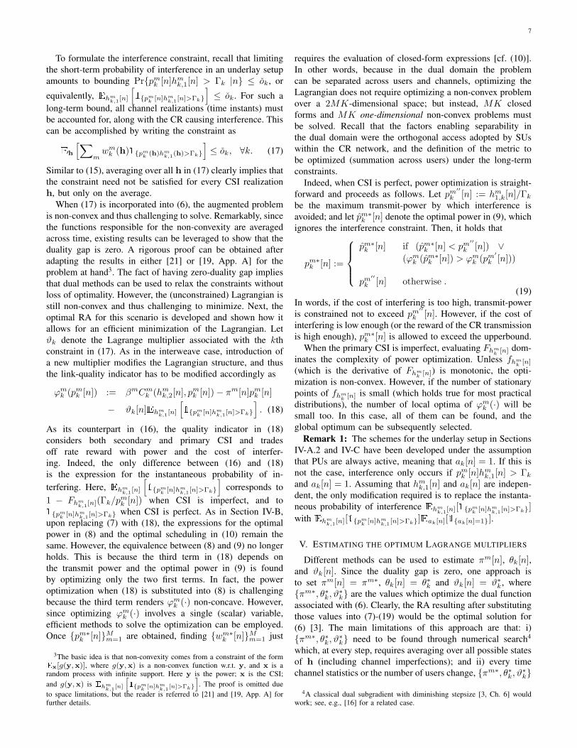
nh = 0,..., Nh−1. The following three S4), S5) and S6) are thecounterparts of S1), S2) and S3) under a long-term interferenceconstraint (LTIC). For further comparison, three more areconsidered: S7) a scheme with no instantaneous informationof the primary CSI, since it relies only on statistical CSI [1],[2]; S8) a scheme that solves (6) ignoring the interferenceconstraints [17]; and S9) a scheme that accounts for CSIimperfections, and solves (6) guaranteing that the averageinterfering power at the PUs is less than Γk [18], [27].

The results corroborate the analytical claims and illus-trate the advantages of the developed algorithms. The novelschemes satisfy the constraints, while those ignoring CSIerrors violate them; and outperform the suboptimal schemes,especially the one based on statistical knowledge of theCR-to-PU channels. It is worth noticing how S2 (long-termconstraint) yields a higher maximum than S1 (short-term).Indeed, S1 over-satisfies the long-term interference constraint,while S2 satisfies the constraint tightly. Finally, the resultsconfirm that the probability of interference estimated by thenovel algorithms using the stochastic updates of the beliefstate corresponds to the actual one. Since our results guaranteethat the long-term constraints are satisfied as n → ∞, smalldiscrepancies may occur when the number of simulated timeinstants is not high enough.

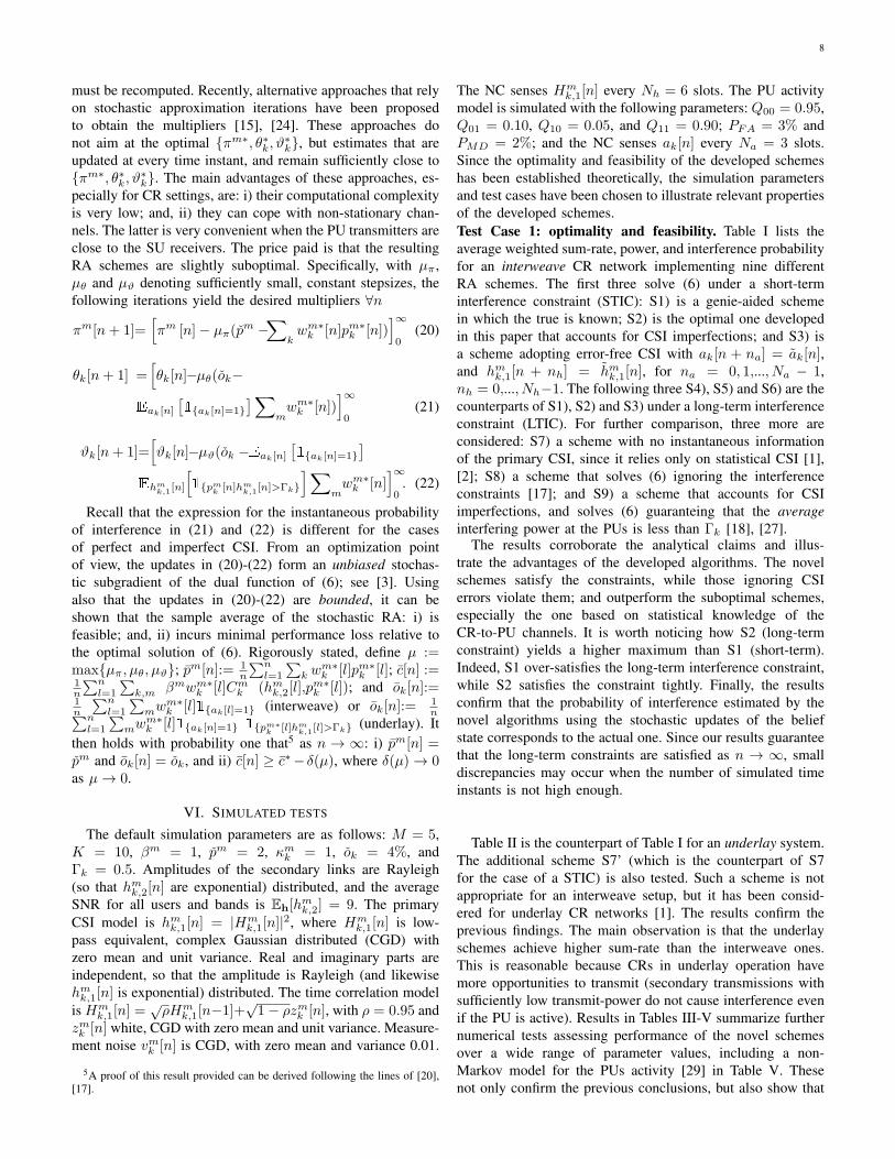
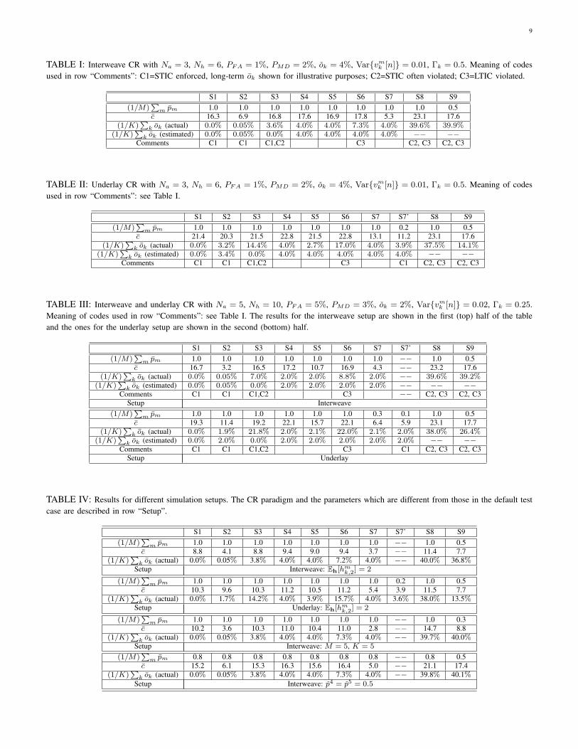
Table II is the counterpart of Table I for an underlay system.The additional scheme S7’ (which is the counterpart of S7for the case of a STIC) is also tested. Such a scheme is notappropriate for an interweave setup, but it has been consid-ered for underlay CR networks [1]. The results confirm theprevious findings. The main observation is that the underlayschemes achieve higher sum-rate than the interweave ones.This is reasonable because CRs in underlay operation havemore opportunities to transmit (secondary transmissions withsufficiently low transmit-power do not cause interference evenif the PU is active). Results in Tables III-V summarize furthernumerical tests assessing performance of the novel schemesover a wide range of parameter values, including a non-Markov model for the PUs activity [29] in Table V. Thesenot only confirm the previous conclusions, but also show that

9

TABLE I: Interweave CR with Na = 3, Nh = 6, PFA = 1%, PMD = 2%, ok = 4%, Var{vmk [n]} = 0.01, Γk = 0.5. Meaning of codesused in row “Comments”: C1=STIC enforced, long-term ok shown for illustrative purposes; C2=STIC often violated; C3=LTIC violated.

S1 S2 S3 S4 S5 S6 S7 S8 S9(1/M)

∑m pm 1.0 1.0 1.0 1.0 1.0 1.0 1.0 1.0 0.5

c 16.3 6.9 16.8 17.6 16.9 17.8 5.3 23.1 17.6(1/K)

∑k ok (actual) 0.0% 0.05% 3.6% 4.0% 4.0% 7.3% 4.0% 39.6% 39.9%

(1/K)∑

k ok (estimated) 0.0% 0.05% 0.0% 4.0% 4.0% 4.0% 4.0% −− −−Comments C1 C1 C1,C2 C3 C2, C3 C2, C3

TABLE II: Underlay CR with Na = 3, Nh = 6, PFA = 1%, PMD = 2%, ok = 4%, Var{vmk [n]} = 0.01, Γk = 0.5. Meaning of codesused in row “Comments”: see Table I.

S1 S2 S3 S4 S5 S6 S7 S7’ S8 S9(1/M)

∑m pm 1.0 1.0 1.0 1.0 1.0 1.0 1.0 0.2 1.0 0.5

c 21.4 20.3 21.5 22.8 21.5 22.8 13.1 11.2 23.1 17.6(1/K)

∑k ok (actual) 0.0% 3.2% 14.4% 4.0% 2.7% 17.0% 4.0% 3.9% 37.5% 14.1%

(1/K)∑

k ok (estimated) 0.0% 3.4% 0.0% 4.0% 4.0% 4.0% 4.0% 4.0% −− −−Comments C1 C1 C1,C2 C3 C1 C2, C3 C2, C3

TABLE III: Interweave and underlay CR with Na = 5, Nh = 10, PFA = 5%, PMD = 3%, ok = 2%, Var{vmk [n]} = 0.02, Γk = 0.25.Meaning of codes used in row “Comments”: see Table I. The results for the interweave setup are shown in the first (top) half of the tableand the ones for the underlay setup are shown in the second (bottom) half.

S1 S2 S3 S4 S5 S6 S7 S7’ S8 S9(1/M)

∑m pm 1.0 1.0 1.0 1.0 1.0 1.0 1.0 −− 1.0 0.5

c 16.7 3.2 16.5 17.2 10.7 16.9 4.3 −− 23.2 17.6(1/K)

∑k ok (actual) 0.0% 0.05% 7.0% 2.0% 2.0% 8.8% 2.0% −− 39.6% 39.2%

(1/K)∑

k ok (estimated) 0.0% 0.05% 0.0% 2.0% 2.0% 2.0% 2.0% −− −− −−Comments C1 C1 C1,C2 C3 −− C2, C3 C2, C3

Setup Interweave(1/M)

∑m pm 1.0 1.0 1.0 1.0 1.0 1.0 0.3 0.1 1.0 0.5

c 19.3 11.4 19.2 22.1 15.7 22.1 6.4 5.9 23.1 17.7(1/K)

∑k ok (actual) 0.0% 1.9% 21.8% 2.0% 2.1% 22.0% 2.1% 2.0% 38.0% 26.4%

(1/K)∑

k ok (estimated) 0.0% 2.0% 0.0% 2.0% 2.0% 2.0% 2.0% 2.0% −− −−Comments C1 C1 C1,C2 C3 C1 C2, C3 C2, C3

Setup Underlay

TABLE IV: Results for different simulation setups. The CR paradigm and the parameters which are different from those in the default testcase are described in row “Setup”.

S1 S2 S3 S4 S5 S6 S7 S7’ S8 S9(1/M)

∑m pm 1.0 1.0 1.0 1.0 1.0 1.0 1.0 −− 1.0 0.5

c 8.8 4.1 8.8 9.4 9.0 9.4 3.7 −− 11.4 7.7(1/K)

∑k ok (actual) 0.0% 0.05% 3.8% 4.0% 4.0% 7.2% 4.0% −− 40.0% 36.8%

Setup Interweave: Eh[hmk,2] = 2

(1/M)∑

m pm 1.0 1.0 1.0 1.0 1.0 1.0 1.0 0.2 1.0 0.5c 10.3 9.6 10.3 11.2 10.5 11.2 5.4 3.9 11.5 7.7

(1/K)∑

k ok (actual) 0.0% 1.7% 14.2% 4.0% 3.9% 15.7% 4.0% 3.6% 38.0% 13.5%Setup Underlay: Eh[h

mk,2] = 2

(1/M)∑

m pm 1.0 1.0 1.0 1.0 1.0 1.0 1.0 −− 1.0 0.3c 10.2 3.6 10.3 11.0 10.4 11.0 2.8 −− 14.7 8.8

(1/K)∑

k ok (actual) 0.0% 0.05% 3.8% 4.0% 4.0% 7.3% 4.0% −− 39.7% 40.0%Setup Interweave: M = 5, K = 5

(1/M)∑

m pm 0.8 0.8 0.8 0.8 0.8 0.8 0.8 −− 0.8 0.5c 15.2 6.1 15.3 16.3 15.6 16.4 5.0 −− 21.1 17.4

(1/K)∑

k ok (actual) 0.0% 0.05% 3.8% 4.0% 4.0% 7.3% 4.0% −− 39.8% 40.1%Setup Interweave: p4 = p5 = 0.5

10

TABLE V: Interweave CR with different models for the activity of the PUs. MM represents the Markov model considered in this paper.PM represents the pareto model considered in [29]. The stationary distribution of ak is the same in both cases. The simulation setup is thesame than that in Table I. Meaning of codes used in row “Comments”: see Table I.

MM: S4 MM: S5 MM: S6 PM: S4 PM: S5 PM: S6(1/M)

∑m pm 1.0 1.0 1.0 1.0 1.0 1.0

c 22.8 21.5 22.8 22.8 21.3 22.8(1/K)

∑k ok (actual) 4.0% 3.6% 17.0% 4.0% 3.4% 17.1%

(1/K)∑

k ok (estimated) 4.0% 4.0% 4.0% 4.0% 4.0% 4.0%Comments C3 C3

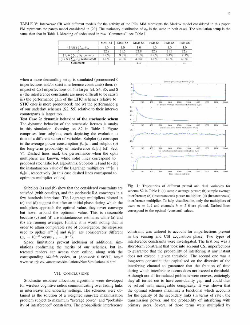
when a more demanding setup is simulated (pronounced CSIimperfections and/or strict interference constraints) then: i) theimpact of CSI imperfections on c is larger (cf. S4, S5, and S6);ii) the interference constraints are more difficult to be satisfied;iii) the performance gain of the LTIC schemes relative to theSTIC ones is more pronounced; and iv) the performance gainof our underlay schemes (S2, S5) relative to their interweavecounterparts is larger too.Test Case 2: dynamic behavior of the stochastic schemes.The dynamic behavior of the stochastic iterates is analyzedin this simulation, focusing on S2 in Table I. Figure 1comprises four subplots, each depicting the evolution overtime of a different subset of variables. Subplot (a) correspondsto the average power consumption pm[n], and subplot (b) tothe long-term probability of interference ok[n] (cf. SectionV). Dashed lines mark the performance when the optimalmultipliers are known, while solid lines correspond to theproposed stochastic RA algorithms. Subplots (c) and (d) depictthe instantaneous value of the Lagrange multipliers πm[n] andθk[n], respectively (in this case dashed lines correspond to theoptimum multiplier values).

Subplots (a) and (b) show that the considered constraints aresatisfied (with equality), and the stochastic RA converges in afew hundreds iterations. The Lagrange multipliers plotted in(c) and (d) suggest that after an initial phase during which themultipliers approach the optimal value, they never convergebut hover around the optimum value. This is reasonablebecause (c) and (d) are instantaneous estimates while (a) and(b) are running averages. Finally, it is worth noting that inorder to attain comparable rate of convergence, the stepsizesused to update πm[n] and θk[n] are considerably different(µπ = 10−2 versus µθ = 10−1).

Space limitations prevent inclusion of additional sim-ulations confirming the merits of our schemes, but in-terested readers can access them online, along with thecorresponding Matlab codes, at [Accessed: 01/05/12] http://www.tsc.urjc.es/∼amarques/simulations/NumSimulations14.html.

VII. CONCLUSIONS

Stochastic resource allocation algorithms were developedfor wireless cognitive radios communicating over fading linksin interweave and underlay settings. The schemes were ob-tained as the solution of a weighted sum-rate maximizationproblem subject to maximum “average power” and “probabil-ity of interference” constraints. The probabilistic interference

0 200 400 600 800 1000 1200 1400 1600 1800 20000

1

2

3

4

5(a) Sample Average Powers: pm[n]

0 200 400 600 800 1000 1200 1400 1600 1800 20000

0.1

0.2

0.3

0.4(b) Sample Average Interference (Estimated): ok [n]

0 200 400 600 800 1000 1200 1400 1600 1800 20000

0.5

1

1.5(c) Instantaneous Power Multipliers: πm[n]

0 200 400 600 800 1000 1200 1400 1600 1800 20000

1

2

3

4(d) Instantaneous Inteference Multipliers: θk[n]

Time iteration index [n]

Fig. 1: Trajectories of different primal and dual variables forscheme S2 in Table I: (a) sample average power; (b) sample averageinterference; (c) (instantaneous) power multiplier; (d) (instantaneous)interference multiplier. To help visualization, only the multipliers ofusers m = 1, 2 and channels k = 5, 6 are plotted. Dashed linescorrespond to the optimal (constant) values.

constraint was tailored to account for imperfections presentin the sensing and CSI acquisition phase. Two types ofinterference constraints were investigated. The first one was ashort-term constraint that took into account CSI imperfectionsto guarantee that the probability of interfering at any instantdoes not exceed a given threshold. The second one was along-term constraint that capitalized on the diversity of theinterfering channel to guarantee that the fraction of timeduring which interference occurs does not exceed a threshold.Although not all formulated problems were convex, enticinglythey all turned out to have zero-duality gap, and could thusbe solved with manageable complexity. It was shown thatthe optimal schemes maximize a functional which accountsfor the quality of the secondary links (in terms of rate), thetransmission power, and the probability of interfering withprimary users. Several of those terms were multiplied by

11

Lagrange multipliers whose value depended on the historyof the system and the requirements of the primary and sec-ondary networks. Stochastic algorithms were introduced to: i)estimate and predict the instantaneous (short-term) probabilityof interference; and, ii) estimate the optimum value of themultipliers. Future directions include accounting for sensingimperfections, as well as jointly optimizing the sensing andresource allocation tasks.

REFERENCES

[1] J.A. Ayala Solares, Z. Rezki, and M. S. Alouini, “Optimal powerallocation of a sensor node under different rate constraints,” Proc. ofIEEE Intl. Conf. on Commun., Otawa, Canada, 2012.

[2] S. Barbarossa, A. Carfagna, S. Sardellitti, M. Omilipo, and L.Pescosolido, “Optimal radio access in femtocell networks based onMarkov modeling of interferers’ activity,” Proc. of IEEE Intl. Conf. onAcoustics, Speech and Signal Process., Prague, Czech Rep., May. 22- 27,2011.

[3] D. Bertsekas, A. Nedic, and A. E. Ozdaglar, Convex Analysis andOptimization, Athena Scientific, 2003.

[4] Y. Chen, Q. Zhao, and A. Swami, “Joint design and separation principlefor opportunistic spectrum access in the presence of sensing errors,” IEEETrans. Inf. Theory, vol. 54, no. 5, pp. 2053-2071, May 2008.

[5] Y. Chen, G. Yu, Z. Zhang, H.-H. Chen, and P. Qiu, “On cognitive radionetworks with opportunistic power control strategies in fading channels,”IEEE Trans. Wireless Commun., vol. 7, no. 7, pp. 2752–2761, Jul. 2008.

[6] E. Dall’Anese, S.-J. Kim, G. B. Giannakis, and S. Pupolin, “Power controlfor cognitive radio networks under channel uncertainty,” IEEE Trans.Wireless Comm., vol. 10, no. 10, pp. 3541–3551, Oct. 2011.

[7] P. Di Lorenzo and S. Barbarossa, “A bio-inspired swarming algorithmfor decentralized access in cognitive radio,” IEEE Trans. Signal Process.,vol. 59, no. 12, pp. 6160 – 6174, Dec. 2011.

[8] A. Ghasemi and E. S. Sousa, “Fundamental limits of spectrum-sharingin fading environments,” IEEE Trans. Wireless Commun., vol. 6, no. 2,pp. 649-658, Feb. 2007.

[9] A. Goldsmith, Wireless Communications, Cambridge Univ. Press, 2005.[10] A. Goldsmith, S. A. Jafar, I. Maric and S. Srinivasa, “Breaking spectrum

gridlock with cognitive radios: An information theoretic perspective,”Proc. IEEE, vol. 97, no. 5, pp. 894–914, May 2009.

[11] S. Haykin, “Cognitive radio: Brain-empowered wireless communica-tions,” IEEE J. Selected Areas Commun., vol. 23, no. 2, pp. 201–220,Feb. 2005.

[12] Y. Y. He and S. Dey, “Power allocation in spectrum sharing cognitiveradio networks with quantized channel information,” IEEE Trans. Com-mun., vol. 59, no. 6, pp. 1644–1656, Jun. 2011.

[13] S. A. Jafar and S. Srinivasa, “Capacity limits of cognitive radio withdistributed and dynamic spectral activity,” IEEE J. Sel. Areas Commun.,vol. 25, no. 3, pp. 529-537, Apr. 2007.

[14] X. Kang, Y.-C. Liang, A. Nallanathan, H. K. Garg, and R. Zhang, “Op-timal power allocation for fading channels in cognitive radio networks:Ergodic capacity and outage capacity,” IEEE Trans. Wireless Commun.,vol. 8, no. 2, pp. 940-950, Feb. 2009.

[15] A. G. Marques, X. Wang, and G. B. Giannakis, “Dynamic resourcemanagement for cognitive radios using limited-rate feedback,” IEEETrans. Signal Process., vol. 57, no. 9, pp. 3651–3666, Sep. 2009.

[16] A. G. Marques, G. B. Giannakis, and J. Ramos, “Optimizing orthogonalmultiple access based on quantized channel state information,” IEEETrans. Signal Process., vol. 59, no. 10, pp. 5023 – 5038, Oct. 2011.

[17] A. G. Marques, L. M. Lopez-Ramos, G. B. Giannakis, J. Ramos, and A.Caamano, “Optimal cross-layer resource allocation in cellular networksusing channel and queue state information,” IEEE Trans. Vehic. Tech.,vol. 61, no. 6, pp. 2789 – 2807, Jul. 2012.

[18] L. Musavian and S. Aissa, “Fundamental capacity limits of cognitiveradio in fading environments with imperfect channel information,” IEEETrans. Commun., vol. 57, no. 11, pp. 3472–3480, Nov. 2009.

[19] K. Rajawat, N. Gatsis, and G. B. Giannakis, “Cross-Layer designsin coded wireless fading networks with multicast,” IEEE/AMC Trans.Networking, vol. 19, no. 5, pp. 1276–1289, Oct. 2011.

[20] A. Ribeiro, “Ergodic stochastic optimization algorithms for wirelesscommunication and networking,” IEEE Trans. Signal Process., vol. 58,no. 12, pp. 6369–6386, Dec. 2010.

[21] A. Ribeiro and G. B. Giannakis, “Separation principles in wirelessnetworking,” IEEE Trans. Info. Theory, vol. 56, no. 9, pp. 4488–4505,Sep. 2010.

[22] H. A. Suraweera, P. J. Smith, and M. Shafi, “Capacity limits and per-formance analysis of cognitive radio with imperfect channel knowledge,”IEEE Trans. Vehic. Tech., vol. 59, no. 4, pp. 1811 – 1822, May 2010.

[23] R. Urgaonkar and M. Neely, “Opportunistic scheduling with reliabilityguarantees in cognitive radio networks,” IEEE Trans. Mobile Comp., vol.8, no. 6, pp.766–777, Jun. 2009.

[24] X. Wang, “Joint sensing-channel selection and power control for cogni-tive radios,” IEEE Trans. Wireless Commun., vol. 10, no. 3, pp. 958–967,Mar. 2011.

[25] X. Wang, G. B. Giannakis, and A. G. Marques, “A unified approachto QoS-guaranteed scheduling for channel-adaptive wireless networks,”Proc. IEEE, vol. 95, no. 12, pp. 2410–2431, Dec. 2007.

[26] Q. Zhao and B. M. Sadler, “A survey of dynamic spectrum access,”IEEE Signal Process. Mag., vol. 24, pp. 79-89, May 2007.

[27] R. Zhang, “On peak versus average interference power constraintsfor protecting primary users in cognitive radio networks,” IEEE Trans.Wireless Commun., vol. 8, no. 4, pp. 2112-2120, Apr. 2009.

[28] R. Zhang, Y.-C. Liang, and S. Cui, “Dynamic Resource Allocationin Cognite Radio Networks: A convex optimization perspective,” IEEESignal Process. Mag., vol. 27, no. 5, pp. 102–114, May 2010.

[29] X. Zhang and H. Su, “Opportunistic spectrum sharing schemes forCDMA-based uplink MAC in cognitive radio networks,” IEEE J. Sel.Areas Commun., vol. 29, no. 4, pp. 716-730, Apr. 2011.

Antonio G. Marques (M’07) received the Telecom-munication Engineering degree and the Doctoratedegree (together equivalent to the B.Sc., M.Sc., andPh.D. degrees in electrical engineering), both withhighest honors, from the Carlos III University ofMadrid, Madrid, Spain, in 2002 and 2007, respec-tively.

In 2003, he joined the Department of SignalTheory and Communications, King Juan Carlos Uni-versity, Madrid, Spain, where he currently developshis research and teaching activities as an Associate

Professor. Since 2005, he has also been a Visiting Researcher at the Depart-ment of Electrical Engineering, University of Minnesota, Minneapolis.

His research interests lie in the areas of communication theory, signal pro-cessing, and networking. His current research focuses on stochastic resourceallocation and network optimization, cognitive radios, and wireless ad hocand sensor networks.

Dr. Marques’ work has been awarded in several conferences and workshops.

Luis M. Lopez-Ramos (S’10) received the B.Sc.degree (with highest honors) in telecommunicationsengineering from the King Juan Carlos Universityof Madrid, Madrid, Spain, in 2010. He is currentlyworking toward the M.Sc. degree in multimediaand communications with Carlos III University ofMadrid. Since then, he has worked as a ResearchAssistant at the Department of Signal Theory andCommunications, King Juan Carlos University. Hisresearch interests include signal processing for wire-less networks, computer vision, cognitive radios and

stochastic resource allocation schemes.

12

G. B. Giannakis (Fellow’97) received his Diplomain Electrical Engr. from the Ntl. Tech. Univ. ofAthens, Greece, 1981. From 1982 to 1986 he waswith the Univ. of Southern California (USC), wherehe received his MSc. in Electrical Engineering,1983, MSc. in Mathematics, 1986, and Ph.D. inElectrical Engr., 1986. Since 1999 he has been aprofessor with the Univ. of Minnesota, where he nowholds an ADC Chair in Wireless Telecommunica-tions in the ECE Department, and serves as directorof the Digital Technology Center.

His general interests span the areas of communications, networking andstatistical signal processing - subjects on which he has published more than325 journal papers, 525 conference papers, 20 book chapters, two editedbooks and two research monographs. Current research focuses on compressivesensing, cognitive radios, cross-layer designs, wireless sensors, social andpower grid networks. He is the (co-) inventor of 21 patents issued, and the(co-) recipient of 8 best paper awards from the IEEE Signal Processing (SP)and Communications Societies, including the G. Marconi Prize Paper Awardin Wireless Communications. He also received Technical Achievement Awardsfrom the SP Society (2000), from EURASIP (2005), a Young Faculty TeachingAward, and the G. W. Taylor Award for Distinguished Research from theUniversity of Minnesota. He is a Fellow of EURASIP, and has served theIEEE in a number of posts, including that of a Distinguished Lecturer for theIEEE-SP Society.

Javier Ramos received the B.Sc. and M.Sc. degreesin telecommunications engineering from the Poly-technic University of Madrid, Madrid, Spain, andthe Ph.D. degree in 1995. Between 1992 and 1995,he was involved with several research projects withPurdue University, West Lafayette, IN, working onsignal processing for communications. In 1996, hewas a Postdoctoral Research Associate with PurdueUniversity. From 1997 to 2003, he was an AssociateProfessor with Carlos III University of Madrid.Since 2003, has been with the King Juan Carlos

University, Madrid, where he is currently a Professor and the Dean of theSchool of Telecommunications Engineering. His research interests includebroadband wireless services and technologies and distributed sensing. Dr.Ramos received the Ericsson Award for the Best Ph.D. Dissertation on MobileCommunications in 1996.