resource allocation in heterogeneous scenarios · pdf fileresource allocation in heterogeneous...
TRANSCRIPT

Resource Allocation in HeterogeneousScenarios
vorgelegt von
Diplom-Ingenieur
Ingmar Blau
aus Uberlingen
Von der Fakultat IV - Elektrotechnik und Informatik
der Technischen Universitat Berlin
zur Erlangung des akademischen Grades
Doktor der Ingenieurwissenschaften
- Dr.-Ing. -
genehmigte Dissertation
Promotionsausschuss:
Vorsitzender: Prof. Dr.-Ing. Adam Wolisz
Berichter: Prof. Dr.-Ing. Dr. rer. nat. Holger Boche
Berichter: Prof. Dr.-Ing. Hans Dieter Schotten
Berichter: Dr.-Ing. habil. Gerhard Wunder
Tag der wissenschaftlichen Aussprache: 09.02.2010
Berlin 2010
D 83


Zusammenfassung
Diese Arbeit befasst sich mit der Ressourcenzuweisung und Luftschnittstellenauswahl in draht-
losen, heterogenen Mehrzellsystemen. Sie spiegelt dabei ein Geschaftsmodel wider, in dem
ein Betreiber mehrere Mobilfunknetze mit uberlappender Netzabdeckung steuert und die Frei-
heit besitzt Nutzer einem System seiner Wahl zuzuweisen. Last-basierte Auswahlstrategien nut-
zen diesen Freiheitsgrad um Uberlastungssituationen in einer Luftschnittstelle auszugleichen,
falls in einem uberlappenden System noch genugend Ressourcen zur Verfugung stehen. Diese
Ansatze sind weit verbreitet, jedoch vernachlassigen die meisten wichtige Diversitatsquellen:
Unterschiedliche Ubertragungstechnologien, Tragerfrequenzen, Kodierungs- und Modulations-
verfahren fuhren dazu, dass Systeme Nutzer mit unterschiedlicher Effizienz unterstutzen. Die-
se wird dabei maßgeblich von der angefragten Dienstklasse und den Kanaleigenschaften der
Nutzer beeinflusst und ist meißt unabhangig von der Systemlast. Hauptziel der Arbeit ist die
Analyse, wie solche Effekte optimal fur die Ressourcenallokation ausgenutzt werden konnen
und welche Gewinne sich hierdurch erreichen lassen.
Im ersten Teil werden unter Anwendung der Dualitatstheorie ein analytisches Modell sowie
Regeln zur optimalen Ressourcenzuweisung in langsam veranderlichen Szenarien hergeleitet.
Die Untersuchungen sind hierbei auf interferenzbegrenzte Systeme und solche mit orthogona-
ler Ressourcenzuweisung wie z.B. UMTS und GSM beschrankt. Weiterhin werden dezentral
operierende Algorithmen entwickelt. Diese sind an den nur eingeschrankt moglichen Signali-
sierungsaustausch zwischen Nutzern und Basisstationen angepasst und maximieren die Anzahl
unterstutzbarer Nutzer oder allgemeine Nutzenfunktionen.
Danach erfolgt die Erweiterung des Ansatzes fur Systeme die sich als parallele Ubertragungs-
kanale modellieren lassen, wie z.B. OFDM. Eine neue Klasse von Nutzenfunktionen wird abge-
leitet, die es erlaubt das im allgemeinen nicht konvexe Optimierungsproblem der Nutzenfunk-
tionsmaximierung konvex darzustellen. Die neue Klasse schließt hierbei eine bereits bekannte,
Log-konvexe, Nutzenklasse mit ein.
Im letzten Abschnitt werden der Einfluss von sich schnell verandernden Kanalen und die
Unkenntnis ihrer Wahrscheinlichkeitsdichtefunktionen auf die optimale Nutzerallokation un-
tersucht. Unter der Annahme, dass alle Luftschnittstellen uber Warteschlangenpuffer verfugen
und dass Nutzenfunktionen in Abhangigkeit von Erwartungswerten formuliert sind, werden Al-
gorithmen entwickelt, die die Nutzenfunktionen eines heterogenen Systems maximieren. Aus-
schlaggebend ist hierbei die geschickte Dimensionierung der Flusskontrolle der Datenpakete.
i

ii
Sie ist so gestaltet, dass sich die Puffer wie duale Parameter einer stochastischen Subgradienten-
methode verhalten und dass durch geeignete Parameterwahl die Paketverzogerung der Nutzer
eingestellt werden kann.

Abstract
In this thesis, resource allocation as well as air interface selection in heterogeneous wireless
multi-cell scenarios are covered. These scenarios correspond to the business case where an
operator is in charge of multiple wireless systems with overlapping coverage and, presuming
that service requests can be supported in several underlying radio access networks, has the free-
dom to assign users to an air interface of its choice. Load balancing schemes, which are widely
used, exploit this freedom in order to prevent overload situations in one technology in case suffi-
cient resources are available in an alternative one. However, most of them neglect an important
source of diversity: air interface specific technologies, carrier frequencies, modulation and cod-
ing schemes provoke that some radio access networks are better suited to support users with
certain channel characteristics and service requests than others, often independent of network
loads. This work analyzes how these effects can be exploited in an optimum way and which
gains can be achieved.
In the first part of the thesis, an analytic model and close to optimum assignment rules for
slowly varying environments are derived based on duality theory. It covers interference limited
air interfaces and those with orthogonal resources such as UMTS and GSM. Decentralized
close to optimum algorithms which are adapted to the limited information exchange between
different technologies and which maximize performance measures such as the weighted number
of assignable users or general system utilities are developed.
The analysis is then extended to radio air interfaces which can be described as parallel
broadcast channels such as OFDM. There, a new class of utility functions is proposed which
guarantees existence of a convex representation of the generally non-convex utility maximiza-
tion problem. The new utility class thereby encloses a known log-convexity class.
In the last chapter the influence of quickly changing environments and ignorance of the
channels’ probability density functions is investigated. There, assuming that the heterogeneous
system’s underlying air interfaces are equipped with queues and that the performance metric is
formulated with respect to time averages, algorithms that maximize the scenario’s sum utility
are derived. Hereby, a flow control is designed which causes the queues to evolve similarly
to dual parameters of a stochastic subgradient procedure and, using a special parameterization,
allows to individually balance users’ delays.
iii


Acknowledgment
I would like to express my sincere gratitude to my advisor, Prof. Holger Boche. He gave
me the opportunity to work at the Fraunhofer German Sino Lab for Mobile communications
(MCI), which I experienced as a stimulating research environment with excellent conditions. I
am very grateful to Prof. Hans Schotten, who spent his valuable time to act as second referee
and reader of this thesis. My deepest gratitude goes to Dr. Gerhard Wunder. His thoughtful
guidance, caring supervision, encouragement and critics was from essential importance for me
to accomplish this thesis.
I am also grateful to all my colleagues at MCI, Heinrich Hertz Institut (HHI) and Technische
Universitat Berlin, who were always open for informative discussions. My special thanks here
go to Dr. Thomas Michel, Dr. Peter Jung and Dr. Nicola Vucic.
My most gratitude goes to my parents for their support. And last, but far from least, I
would like to thank Karolin Blattmann. Without her never ending support, understanding and
encouragement, this work would not have come to fruition.
v


Table of Contents
1 Introduction 1
1.1 Related Work . . . . . . . . . . . . . . . . . . . . . . . . . . . . . . . . . . . 1
1.2 Outline of the Thesis . . . . . . . . . . . . . . . . . . . . . . . . . . . . . . . 3
1.3 Notation . . . . . . . . . . . . . . . . . . . . . . . . . . . . . . . . . . . . . . 5
2 Heterogeneous Access Management in Slowly Varying Environments 7
2.1 System Model . . . . . . . . . . . . . . . . . . . . . . . . . . . . . . . . . . . 7
2.1.1 Fixed Versus Time Variant System Model . . . . . . . . . . . . . . . . 8
2.1.2 Air Interfaces . . . . . . . . . . . . . . . . . . . . . . . . . . . . . . . 9
2.1.3 Service Requests . . . . . . . . . . . . . . . . . . . . . . . . . . . . . 11
2.1.4 Simulation Setup . . . . . . . . . . . . . . . . . . . . . . . . . . . . . 11
2.2 Optimal Service Allocation at Fixed Service Mixes . . . . . . . . . . . . . . . 13
2.2.1 System Model and Definitions . . . . . . . . . . . . . . . . . . . . . . 14
2.2.2 Optimization Problem and Dual Representation . . . . . . . . . . . . . 15
2.2.3 Minimizing the Dual Function Using Subgradients . . . . . . . . . . . 17
2.2.4 Ellipsoid Method . . . . . . . . . . . . . . . . . . . . . . . . . . . . . 19
2.2.5 User Capacity Regions . . . . . . . . . . . . . . . . . . . . . . . . . . 19
2.2.6 Simulation Results . . . . . . . . . . . . . . . . . . . . . . . . . . . . 26
2.3 Cost Based User Assignment for Services with Minimum QoS Requirements . 29
2.3.1 Cost and Feasibility Regions . . . . . . . . . . . . . . . . . . . . . . . 30
2.3.2 Optimization Problem and Relaxation . . . . . . . . . . . . . . . . . . 31
2.3.3 Bounds . . . . . . . . . . . . . . . . . . . . . . . . . . . . . . . . . . 33
2.3.4 Interpretation of the Lagrange Multipliers . . . . . . . . . . . . . . . . 38
2.3.5 Cost Based Algorithm . . . . . . . . . . . . . . . . . . . . . . . . . . 39
2.3.6 Simulation Results for Static Scenarios . . . . . . . . . . . . . . . . . 43
2.3.7 Simplex Algorithm . . . . . . . . . . . . . . . . . . . . . . . . . . . . 44
2.3.8 Simulations in Varying Environments . . . . . . . . . . . . . . . . . . 47
2.4 Distributed Utility Maximization . . . . . . . . . . . . . . . . . . . . . . . . . 49
2.4.1 Utility Concept and α-Proportional Fairness . . . . . . . . . . . . . . . 50
2.4.2 Rate Approximation in Interference Limited RANs . . . . . . . . . . . 52
2.4.3 Problem Formulation . . . . . . . . . . . . . . . . . . . . . . . . . . . 53
2.4.4 Decentralized Algorithms . . . . . . . . . . . . . . . . . . . . . . . . 58
vii

viii TABLE OF CONTENTS
2.4.5 Soft QoS Support . . . . . . . . . . . . . . . . . . . . . . . . . . . . . 63
2.4.6 Simulation Results . . . . . . . . . . . . . . . . . . . . . . . . . . . . 64
2.5 Summary . . . . . . . . . . . . . . . . . . . . . . . . . . . . . . . . . . . . . 68
3 MSE Based Utility Maximization in Parallel Broadcast Channels 71
3.1 Introduction . . . . . . . . . . . . . . . . . . . . . . . . . . . . . . . . . . . . 71
3.2 System Model . . . . . . . . . . . . . . . . . . . . . . . . . . . . . . . . . . . 73
3.3 Problem Statement . . . . . . . . . . . . . . . . . . . . . . . . . . . . . . . . 74
3.4 Utility Optimization Based on CMSEs . . . . . . . . . . . . . . . . . . . . . . 75
3.4.1 Multiuser CMSE Region . . . . . . . . . . . . . . . . . . . . . . . . . 75
3.4.2 Consequences for the MIMO MSE Region . . . . . . . . . . . . . . . 79
3.4.3 Convexity of the BC Utility Region . . . . . . . . . . . . . . . . . . . 80
3.4.4 A New Class of Utility Functions: the Square Root Law . . . . . . . . 82
3.5 Minimum Sum Power under CMSE Constraints . . . . . . . . . . . . . . . . . 85
3.6 Algorithms and Simulation Results . . . . . . . . . . . . . . . . . . . . . . . . 85
3.6.1 Sum Utility Maximization . . . . . . . . . . . . . . . . . . . . . . . . 86
3.6.2 Sum Power Minimization . . . . . . . . . . . . . . . . . . . . . . . . 88
3.6.3 Simulation Results . . . . . . . . . . . . . . . . . . . . . . . . . . . . 89
3.7 Suboptimum Resource Allocation in PBCs . . . . . . . . . . . . . . . . . . . . 89
3.8 PBCs in Heterogeneous Multi-Air Interface Networks . . . . . . . . . . . . . . 91
3.9 Summary . . . . . . . . . . . . . . . . . . . . . . . . . . . . . . . . . . . . . 96
4 Queue Based Utility Maximization in Heterogeneous Wireless Scenarios 99
4.1 System Model . . . . . . . . . . . . . . . . . . . . . . . . . . . . . . . . . . . 101
4.2 Problem Formulation . . . . . . . . . . . . . . . . . . . . . . . . . . . . . . . 103
4.3 Queue Based Flow Control and Scheduling . . . . . . . . . . . . . . . . . . . 103
4.4 Stochastic Subgradient Interpretation . . . . . . . . . . . . . . . . . . . . . . 104
4.5 Tuning of Equilibrium Buffer States . . . . . . . . . . . . . . . . . . . . . . . 109
4.6 Adaptive Tuning of Queues . . . . . . . . . . . . . . . . . . . . . . . . . . . . 111
4.7 Simulation Results . . . . . . . . . . . . . . . . . . . . . . . . . . . . . . . . 112
4.8 Summary . . . . . . . . . . . . . . . . . . . . . . . . . . . . . . . . . . . . . 117
5 Conclusions and Outlook 119
5.1 Conclusions . . . . . . . . . . . . . . . . . . . . . . . . . . . . . . . . . . . . 119
5.2 Outlook . . . . . . . . . . . . . . . . . . . . . . . . . . . . . . . . . . . . . . 122
Acronyms 123
Publications 125
Bibliography 127

List of Figures
2.1 Playground of heterogeneous GSM, UMTS scenario . . . . . . . . . . . . . . 9
2.2 SINR-rate mapping curves for UMTS and GSM/EDGE . . . . . . . . . . . . . 13
2.3 Exemplary capacity region for 2 RANs and 2 services . . . . . . . . . . . . . . 17
2.4 Approximation of user capacity regions . . . . . . . . . . . . . . . . . . . . . 24
2.5 Performance of Algorithm 1 . . . . . . . . . . . . . . . . . . . . . . . . . . . 27
2.6 Simulated capacity regions for UMTS and GSM/EDGE cells . . . . . . . . . . 28
2.7 Comparison of service aware and unaware load balancing . . . . . . . . . . . . 29
2.8 Illustration of split user bound . . . . . . . . . . . . . . . . . . . . . . . . . . 37
2.9 CDF of assignable users for cost based vs. load balancing algorithm . . . . . . 44
2.10 Number of supported users in a heterogeneous UMTS/GSM scenario . . . . . . 48
2.11 UMTS resource-rate mapping: quality of linear approximation . . . . . . . . . 53
2.12 Utility curves for BE services . . . . . . . . . . . . . . . . . . . . . . . . . . . 64
2.13 Performance of decentralized utility maximization algorithm . . . . . . . . . . 66
2.14 Optimal air interface selection on the playground . . . . . . . . . . . . . . . . 67
2.15 Sum utility and upper bound with 6 dB slow-fading. . . . . . . . . . . . . . . . 68
3.1 Illustration of Lemma 2’s proof . . . . . . . . . . . . . . . . . . . . . . . . . . 78
3.2 Illustration of an exemplary complementary BC MSE region . . . . . . . . . . 79
3.3 Complementary MSE MAC region . . . . . . . . . . . . . . . . . . . . . . . . 80
3.4 Function principle of the gradient projection algorithm . . . . . . . . . . . . . 86
3.5 Convergence speed of Algorithm 7 . . . . . . . . . . . . . . . . . . . . . . . . 89
3.6 Convergence speed of Algorithm 8 . . . . . . . . . . . . . . . . . . . . . . . . 90
3.7 Achievable boundary points on non-convex rate regions . . . . . . . . . . . . . 94
3.8 Influence of the subcarriers’ number on the activation of users . . . . . . . . . 96
4.1 System model of heterogeneous scenarios with queues . . . . . . . . . . . . . 102
4.2 Sum utility: influence of step size and delay on the algorithms’ performance . . 114
4.3 Influence of step size s(t) and k on the evolution of queues of Algorithm 9 . . . 115
4.4 Influence of step size s(t) and k on delays of RAT 2 of Algorithm 9 . . . . . . . 115
4.5 Influence of f (w, q(t)) = wq(t) on queues and delays for Algorithm 10 . . . . . 116
4.6 Influence of adaptive weight control in Algorithm 11 . . . . . . . . . . . . . . 117
ix


List of Tables
2.1 Standard parameters used in the MRRM Simulator. . . . . . . . . . . . . . . . 12
4.1 Average data rates in dependence of distance for WiMAX and HSDPA . . . . . 113
xi


Chapter 1
Introduction
Today’s wireless communication infrastructure is characterized by a heterogeneous compila-
tion of different Radio Access Technologies (RATs), each designed according to state-of-the-
art transmission concepts and tailored to actual business models at the time of establishment.
Although operators are continuously introducing new technologies to the market, there is still a
strong interest in exploiting legacy systems efficiently, not only to increase the return on invest
but also to allow for gradual employment of new wireless systems. Accompanied by multi-
standard capabilities of modern terminals this opens up the way for exploiting a new degree
of diversity for resource assignment: operators have now the freedom to support users by a
radio access technology of their choice presuming that users are within the coverage of mul-
tiple wireless accesses all supporting the requested service. The optimum exploitation of this
characteristic, denoted air interface diversity in the following, will be investigated in this thesis.
1.1 Related Work
Heterogeneous resource management appears in versatile forms in the literature and is closely
related to resource allocation problems of individual radio access technologies and cross-layer
optimization [SRK03]. A wide variety of strategies and rich mathematical theory, includ-
ing convex [Ber95a], stochastic [KY03] and global optimization [HT93], dynamic program-
ming [Ber95b] and game theory [FT91] has been applied to tackle similar resource assignment
problems. In addition, classic engineering approaches exist, which are tailored to the necessities
of specific technologies and scenarios.
An early, practical example allowing exploitation of air interface diversity is given by the
Third Generation Partnership Project (3GPP) standard for the second and third generation of
wireless communication systems, i.e. Global System for Mobile Communications (GSM)/Enhanced
Data Rates for GSM Evolution (EDGE) and the Universal Mobile Telecommunications System
(UMTS)/High Speed Downlink Packet Access (HSDPA) [Net], [3GP08]. This standard pro-
vides mechanisms to exchange load information and allows for Inter-system Hand-overs (ISHOs)
1

2 Chapter 1. Introduction
between the two heterogeneous air interfaces. In the literature these mechanisms are commonly
used to avoid overload situations in a wireless technology, generated by asymmetric requests
or system capacities, by initiating ISHOs or directing call setup requests to alternative radio
access technologies where still sufficient resources are available. Many versions of these load
balancing and heterogeneous resource management strategies for services with fixed rate re-
quirements such as voice and/or elastic data traffic exist, among those [PDJMT04], [Hil05],
[PDKS06], [PRSA07]. The latter aim at achieving balanced exploitation of resources thereby
reducing blocking, dropping or outage probabilities. However, they neglect the fact that the sum
load in a heterogeneous scenario may depend on the compilation of user assignments in indi-
vidual RATs and that the network selection should depend on the traffic characteristics, radio
link quality and user preferences [ZM04].
One of the first attempts to extend pure load balancing to a strategy considering these effects
for the RAT selection is presented in [FZ05]. There, the authors observe that RATs support
service classes with different efficiencies and that, for maximizing the total number of assignable
users at a predetermined service compilation, optimum service mixes exist for each technology.
A similar observation is exploited in [HPZ05] for maximizing a heterogeneous networks’s sum
utility. Linear programming is applied there to formulate an analytic model and an algorithmic
solution based on average service costs in each technology. On the contrary, the fact that the
suitability of air interfaces may depend on the channel gain and therefore on users’ positions
is exploited in [PRSA06] and a service independent path loss threshold for the air interface
selection in a heterogeneous UMTS/GSM scenario is proposed. However, none of the works
mentioned above considers both, channel and service class, for the Radio Access Network
(RAN) selection; a drawback which is managed in this thesis.
While the latter approaches focus on static scenarios, a greedy policy including service and
channel dependent costs is presented in [CC06] for the RAT selection in dynamic settings us-
ing graph theory. Dynamic programming represents a promising framework for integrating the
stochastic nature of the channel, mobility and the request situation into the RAT selection pro-
cess as presented in the works [SNLW08] and [FL07]. It additionally allows the incorporation
of ISHO costs in the problem formulation. Solving dynamic problems, however, is expensive
in terms of computational cost and thus better suited for offline calculations. Especially, in case
the channel state is considered in the optimization, the state space quickly becomes extremely
large and requires efficient clustering for its management [BW09].
Game theory, used e.g. in [HEBJ08], represents an attractive methodology when distributed
operation is an algorithms’ key requirement and if only limited signaling information can be
exchanged between air interfaces. Nevertheless, often only convergence to equilibria which are
not optimal from a network perspective is achieved.
Since heterogeneous access selection embeds the resource allocation of underlying air inter-
faces, the literature on resource assignment strategies of the comprised technologies is closely
related to it. Results on network utility maximization in static, interference limited air-interfaces

1.2. Outline of the Thesis 3
are presented in [SWB06], [Chi05a]. There, prerequisites, which are loosened for the subclass
of Parallel Broadcast Channels (PBCs) in this thesis, for the convexity of sum utility regions
and distributed algorithms for the resource assignment are derived. Those strategies heavily ex-
ploit convex reparameterizations of the underlying problem and duality theory [PC06]. Based
on super-modular game theory, similar findings as in [SWB06] are also presented in [HBH06].
Resource assignment in air interfaces with orthogonal resources such as Time Division Multi-
ple Access (TDMA), Frequency Division Multiple Access (FDMA) or Orthogonal Frequency
Division Multiplex (OFDM) can often be formulated or approximated as convex optimization
problems [SL05a], [SMC06]. Related work on load balancing and cell-selection algorithms in
multi-cell Wireless Local Area Network (WLAN) networks using convex optimization theory
can be found in [CRdV06].
Likewise, works on utility maximization in time variant scenarios where the optimization
metrics are formulated as time averages as in [ES07], [NML08] and [KW04], constitute a valu-
able basis for this thesis. The former two papers suggest queue based scheduling and flow
control policies and prove close to optimality of the resource allocation by Lyapunov tech-
niques. The latter applies stochastic optimization theory in a setup without queues to achieve
proportional fair assignments; both models are combined in the thesis allowing to tune the
users’ delays in addition to maximizing the sum utility in a heterogeneous scenario as will be
explained in more detail in the following section.
1.2 Outline of the Thesis
Using the literature cited in the precedent section as point of origin, this thesis covers the de-
sign and analysis of resource allocation strategies for wireless scenarios consisting of multiple,
heterogeneous radio access technologies. All RANs are assumed to operate orthogonal to each
other, have (partly) overlapping coverage and terminals to support all technologies. Throughout
the work a top down approach is chosen: starting from a practically relevant problem for-
mulation it is aimed to derive general, analytic and practically feasible solutions based on a
mathematically sound framework.
The thesis is divided into three main chapters. Following the introduction, Chapter 2 deals
with the problem of RAT and cell selection as well as resource allocation in heterogeneous
scenarios consisting of air-interfaces with orthogonal and interference limited resources in
slowly varying environments. Algorithms are derived for service requests with fixed Quality
of Service (QoS) requirements for maximizing either the total number of assignable users at a
given service mix or the weighted number of assignable users in multi-RAN networks. Hereby,
convex optimization and continuous relaxation techniques are applied; for the latter bounds on
the maximum degradation from the optimum are deduced. The algorithmic framework is then
further extended to include services with flexible data rates such as Best Effort (BE) data traffic
by introducing a general utility concept. The proposed algorithm’s completely decentralized
4 Chapter 1. Introduction
operation, low signaling efforts between the RANs’ Base Stations (BSs) and users in addition
to close to optimum operation make it a promising strategy for practical applications. The
performance of the derived algorithms is evaluated in simulations for a heterogeneous UMTS
GSM/EDGE scenario.
Chapter 3 focuses on the resource allocation in PBCs. PBCs are suitable for either modeling
heterogeneous scenarios with potentially coupled resource constraints between different tech-
nologies; they may also serve as general descriptions of underlying radio access technologies
such as OFDM, where each channel represents a subcarrier. In the first part of the chapter the
square-root utility class is derived. It allows the formulation of a convex reparametrization of
the in general non-convex utility maximization as well as the dual sum power minimization
problem in PBCs and represents an extension of the log-convex class in [SWB06] which is a
strict subset of the former. For utility functions of the square-root class algorithmic solutions
in the non-convex domain are presented which are shown to converge to the global optimum in
polynomial time. The second part presents a more practically oriented assignment procedure in
heterogeneous scenarios including OFDM based technologies thereby extending the approach
in [SMC06]: confining assignments to those with no more than one user per subcarrier, good
approximations for the modified problem exist for arbitrary concave and strictly increasing util-
ities. Aside, the effect of constraining each user’s activity to one air interface at a time on the
performance is discussed.
The influence of the time variant nature of the channel on the heterogeneous resource al-
location and air interface diversity in quickly changing environments is covered in Chapter 4.
There, the question of optimum flow control and resource allocation of packet based traffic is
studied in RANs which are equipped with queues and employ scheduling protocols. Instead of
instantaneous utilities, optimized in Chapters 2 and 3, sum utilities depending on average data
rates are covered. An algorithmic concept for utility maximization which learns the ergodic
rate regions over time and bases its decisions for flow control and resource allocation solely
on the instantaneously assigned rates and buffer states is presented. Its optimality is proven by
showing that buffers evolve similarly to dual parameters in an equivalent stochastic optimiza-
tion problem, thereby identifying the queue based procedures proposed in [ES07] and [NML08]
as stochastic subgradient methods with constant step size. Exploiting this observation, queue
based algorithms that mimic stochastic subgradient procedures with adaptable step size and
perform better compared to those with constant step size are designed. In addition, the new
algorithms allow to balance the packets’ delays by basing flow control and scheduling on func-
tions of the buffer states. Thereby, out-of-sequence problems are prevented which may arise if
a user’s packets are routed through different RANs.

1.3. Notation 5
1.3 Notation
Vectors and matrices are denoted by bold letters. Hereby, a vector a is understood as column
vector a = (a1, . . . , aN), N ∈ N and N the set of natural numbers; a matrix A has the form:
A =
A1,1 . . . A1,M
.... . .
...
AI,1 . . . AI,M
The hermitian transpose of a vector or matrix is indicated by (·)H. For vector norms the follow-
ing defintion is introduced:
‖x‖l =
∑
n
|xn|l
1/l
, l ∈ N (1.1)
A vector with all entries equal to one is given by 1 with appropriate size corresponding to
the context. Calligraphic letters M denote sets with cardinality |M| = M and conv(M) their
convex hull. The operator [·]ba is equivalent to max(min(·, b), a) and the expectation of a random
variable is denoted by E[·]. For x ∈ R y = ⌈x⌉ (y = ⌊x⌋) is the smallest (largest) integer
y ∈ N which is larger (smaller) than or equal to x. The summation over sets is defined as
X = ∑
nXn = {x : x =∑
n xn, xn ∈ Xn}. a◦b signifies the Hadamard product and a ≻ (�) ≺ (�)b
element-wise greater (equal) smaller (equal). For the above defined matrix A with real entries
A � 0 is equivalent to A ∈ RI×M+ and A ≻ 0 has the same meaning as A ∈ RI×M
++ for R the set
of real numbers. a−1 = (a−11, . . . , a−1
N ) represents a vector with inverse entries. The composition
of functions is defined by (g ◦ f )(x) := g( f (x)) and for the inverse g−1(x) of function g(x) holds
g(g−1(x)) = x. If not stated differently, log(·) is the natural logarithm and rank(A) the rank of
matrix A.


Chapter 2
Heterogeneous Access Management in
Slowly Varying Environments
This chapter deals with RAT selection and resource allocation in heterogeneous scenarios con-
sisting of air interfaces with interference limited and orthogonal resource assignment. After in-
troducing the system model in Section 2.1 an algorithm for finding the optimum service mixes
in individual cells, which maximize the total supportable arrival rate of calls with fixed QoS
requirements at a given service mix, is derived in Section 2.2. In Section 2.3 the assignments
are improved by considering users’ channel gains in addition to the requested service type for
the resource allocation in order to maximize the weighted sum of assignable users. An opti-
mization framework which includes also services with flexible QoS requirements and operates
in a completely distributed way is then presented in Section 2.4. More detailed introductions
are presented at the beginning of each section which follow after the definition of the general
system model.
2.1 System Model
In this Section a general system model for heterogeneous multi-RAN, multi-service scenarios
is defined which is valid throughout this chapter if not stated differently.
The downlink direction of a wireless scenario where a single operator is in charge of multiple
radio access networks or air interfaces with at least partly overlapping coverage is considered. A
RAN or air interface is defined as the part of the infrastructure in a communication system which
lies between mobile terminals and the core network and implements a RAT. Interchangeably
with term RAT/RAN, originating from the European Telecommunications Standards Institute
(ETSI) [ETS06], the term air interface which is the prevalent term outside of Europe such as in
the Telecommunication Industry Association (TIA) is used. The set of air interfaces is denoted
byA and each air interface may consist of a set of cells or BSsMa, a ∈ A. For ease of notation
the set of all BSs in the heterogeneous scenario is defined byM := ∪a∈AMa independently of
7

8 Chapter 2. Heterogeneous Access Management in Slowly Varying Environments
the underlying technology.
Commercial wireless systems usually operate on individual frequency bands. Thus, orthog-
onality between signals of different air interfaces is a valid assumption and inter-system interfer-
ence can be precluded. However, users may be affected by intra-cell and inter-cell interference
within one radio technology. Assignable resources such as power budgets, subcarriers or time
slots cannot be shared between different BSs. To allow for the coordination of the heterogeneous
user assignment it is assumed that some form of information exchange exists between differ-
ent radio access networks. The latter can be realized by Multiple Radio Management (MRM)
protocols as introduced in [SBEW09]. It is addressed directly in the sections if considered.
The system model is further characterized by defining an area called playground which
lies in the coverage area of at least one air interface of the heterogeneous scenario. Inside the
playground users i ∈ I request services si ∈ S not specifying a desired radio access technology.
Without loss of generality it is assumed that the users are equipped with multi-mode terminals
supporting all radio access technologies a ∈ A and also that each RAN offers all services
s ∈ S. The latter gives operators the freedom to assign users to air interfaces of their choice
in case sufficient resources and coverage is available. The performance gain that is based on
exploiting this freedom is denoted as air interface diversity. Throughout Chapter 2 users may be
assigned to no more than one technology at a time, a characteristic that arises from the separated
infrastructure of different RANs. Nevertheless, multi-RAN operation may be beneficial from a
theoretic perspective, which is shown in Chapters 3 and 4. An exemplary heterogeneous multi-
cell scenario for a GSM/EDGE and UMTS air interface used in most simulations is depicted in
Figure 2.1. More details on the air interfaces are given in Section 2.1.4.
2.1.1 Fixed Versus Time Variant System Model
The characteristics of wireless scenarios, such as channel, user positioning, mobility and re-
quest situation, are usually varying over time. Depending on the frequency and relevance of
these effects a probabilistic system description may be advantageous for close-to-reality mod-
eling. Since analyzing such a probabilistic model often becomes very complex, two different
approaches are used in this chapter: the snapshot model and the probabilistic model. In the
former model it is assumed that the scenario’s variation over time is negligable compared to the
operation time of a policy and validity of a performance measure under investigation, thus jus-
tifying the assumption of fixed channel gains and request situation for analytical modeling. On
the contrary, the probabilistic model is based on a spacial birth and death process of the requests
over time. More precisely, requests of service class s ∈ S emerge corresponding to a Poisson
process with mean measure rs in the scenario. Their duration is assumed to be exponentially
distributed with mean ds and probability density function
f (x) =1
ds
e−x
ds . (2.1)

2.1. System Model 9
Investigation area Movement area
Colocated directional GSM/UMTS BS
Main transmission direction
Figure 2.1: Playground containing 42 GSM and 42 UMTS BSs with directional transceivers
(left). Each red triangle marks the position of each technology’s three directional BSs which
are colocated; the arrows point in the main transmission directions. The hexagons indicate the
theoretic separation into cells, whereby only service requests from users assigned to the yellow
ones are considered for the simulation results. The black rectangle limits the area in which users
move and request services. An exemplary cell with one BS of each technology is shown on the
right.
For this model it is noted that if all requests are accepted the number of users Is in the system
follows a Poisson distribution with probability mass function
P(Is = k) = e−rsds(rsds)
k
k!. (2.2)
The initial position of emerging users is drawn from a uniform distribution over the area of the
playground. It also characterizes the mean of users’ associated channel processes for static re-
quests. Although mobility is not modeled analytically it is considered in simulations in Section
2.2.6 and 2.4.6.
2.1.2 Air Interfaces
The set of air interfaces under consideration is assumed to belong to two subclasses, RANs with
orthogonal resource assignment modes a ∈ Aorth, such as TDMA or FDMA, and interference
limited air interfaces a ∈ Ain f e.g. Code Division Multiple Access (CDMA) based.

10 Chapter 2. Heterogeneous Access Management in Slowly Varying Environments
Orthogonal RANs
For the class of orthogonal systems a fixed transmission power per BS is assumed. The band-
width, i.e. time or frequency slots, is the resource distributable between users. In this class of
systems constant inter-cell interference is considered which is supported by the fact that com-
mercial TDMA systems like GSM/EDGE usually have low frequency reuse; i.e. neighboring
BSs operate on different frequency bands. Thus, inter-cell interference originates only from
further distant BSs and the influence of the users positions within the cell of interest on the
inter-cell interference can be neglected. The Signal to Interference and Noise Ratio (SINR)
between user i ∈ I and a BS m ∈ Ma, a ∈ Aorth of this class
βi,m =gi,mPm
ηorth
∀m ∈ Ma, a ∈ Aorth
thus depends on the channel gain gi,m, the BS power Pm and the sum of the constant inter-cell
interference and the thermal noise variance ηorth, but is independent of the assigned resource.
The amount of bandwidth assigned to user i by BS m is denoted by ti,m. It is limited by the total
distributable bandwidth per BS Tm and the constraint
∑
i∈Iti,m = tm ≤ Tm ∀m ∈ Ma, a ∈ Aorth. (2.3)
Due to the orthogonality of users’ signals and the fact that the bandwidth is the distributable
resource the relation between a user’s data rate Ri,m and the assigned resource is linear for this
class of RANs:
Ri,m = Ri,mti,m ∀i,m ∈ I,Ma, a ∈ Aorth (2.4)
Here, Ri,m := fa(βi,m), m ∈ Ma denotes the feasible link rate per time or frequency slot between
user i and BS m. The function fa(·) represents a positive, non-decreasing SINR-rate mapping
curve corresponding to the coding, modulation and transmission technology of RAN a ∈ Aorth,
which is usually obtained from measurements. The rate should therefore not be confused with
the information theoretic rate but rather be understood as a practical measure which may toler-
ate a certain probability of error. From an information theoretic point of view one could also
substitute the Shannon capacity, which represents an upper bound on the error free transmis-
sion rate, instead. However, the noise plus interference must then follow a Gaussian circularly
symmetric distribution in order to obtain reasonable results.
Interference Limited RANs
In interference limited air interfaces it is assumed that all users share the same bandwidth and
that resources are distributed by means of BSs’ m ∈ Mb, b ∈ Ain f power assignment. The latter

2.1. System Model 11
is limited by a sum power constraint
∑
i∈Ipi,m = Pm ≤ Pm ∀m ∈ Mb, b ∈ Ain f , (2.5)
where pi,m is the non negative power that BS m assigns to user i ∈ I. Users are sensitive to
intra-cell and inter-cell interference in interference limited systems and the SINR between BS
m and user i ∈ I is defined by:
βi,m =gi,m pi,m
ρgi,m
∑
j,i p j,m +∑
n,m gi,nPn + ηin f
m, n ∈ Mb, b ∈ Ain f , i, j ∈ I (2.6)
In (2.6) ηin f is the thermal noise variance and 0 ≤ ρ ≤ 1 denotes a non-orthogonality factor.
It may be used to model reduced inter-cell interference if users are separated through carefully
designed spreading sequences as e.g. in CDMA. A user’s data rate is given as a function of its
SINR in this class of systems:
Ri,m = fb(βi,m), i,m ∈ I,Mb, b ∈ Ain f
Like in Section 2.2.5, fb(·) depends on the transmission technology and is usually obtained from
measurements.
Although the spreading sequences used in the CDMA based UMTS downlink are orthogonal
Walsh codes, their orthogonality is often lost in real world scenarios through time dispersive
channels [PM02]. Based on this fact (2.6) represents a well accepted model also for CDMA
based RANs and is used to model UMTS in this thesis.
2.1.3 Service Requests
All services s ∈ S considered in this chapter can be divided into two classes: those with fixed
QoS constraints and those with elastic requirements. For the former class the QoS constraint
can be mapped to a minimum data rate which has to be guaranteed with fixed probability of
error in the scenario. This class refers to circuit switched services, such as voice traffic, where
a fixed minimum data rate is required and higher data rates do not improve the service quality.
Elastic BE services, on the other hand, are assumed to operate within a range of data rates,
including streaming or data services. Delay and jitter, which are also commonly used in the
definition of QoS measures, are not considered.
2.1.4 Simulation Setup
The simulations in this chapter are restricted to heterogeneous scenarios consisting of one inter-
ference limited air interface UMTS and one orthogonal GSM/EDGE system. All multi-cell sim-
ulations are performed using an event driven Multiple Radio Resource Management (MRRM)

12 Chapter 2. Heterogeneous Access Management in Slowly Varying Environments
Table 2.1: Standard parameters used in the MRRM Simulator.
Max. power UMTS: Pm = 20W
Max. power GSM: Pm = 15W
Time-slots GSM: Tm = 21
Antenna pattern: Sector 90◦ [TR101]
Path loss GSM [dB], (r distance in [m]): gdb = 132.8 + 38 lg(r − 3) [ETS99]
Path loss UMTS [dB]: gdb = 128.1 + 37.6 lg(r − 3) [TR101]
SINR-rate mapping UMTS: Cb = 1.14e9, Db = 8.7e − 4
Thermal noise GSM: −105 dBm
Thermal noise UMTS: −100 dBm
Inter-cell interference GSM: −105 dBm
Orthogonality factor UMTS: ρ = 0.4
Simulator for heterogeneous access management. The C++ based environment was developed
in cooperation with Alcatel-Lucent and supports cellular UMTS/HSDPA, GSM/EDGE air in-
terfaces, a Worldwide Interoperability for Microwave Access (WiMAX) hot-spot and different
service classes such as Voice over Internet Protocol (VoIP), streaming, circuit switched voice
and BE data services. The layout of the simulation scenario consisting of 42 colocated UMTS
and GSM/EDGE cells is shown in Figure 2.1, where on each site, marked by the red triangles,
3 BSs with directional antennas of both RANs are positioned. The distance between the sites
is 2400 m. All RAN specific parameters are listed in Table 2.1. For the UMTS network the
SINR-rate mapping curve from the MRRM Simulator specification [KSB+08] is used. It is
based on link level simulations from [Agi99] and, motivated by the SINR-rate approximations
for adaptive modulation schemes in [Gol05], can be fitted to the analytic expression
fb(β) = Cb log2(1 + Dbβ), (2.7)
which is used in Section 2.4.2. Since for the GSM/EDGE rate mapping no analytic fitting
is needed, in the following analysis the curves from [KSB+08], originating from link level
simulations, are used. Mappings for both air interfaces are depicted in Figure 2.2. In UMTS the
SINR-rate mapping is independent of the service type and limited by a maximum transmission
rate of 384kbit/s. Its observable almost linear shape is exploited in Section 2.4. The data
rate R in Figure 2.2 (right) denotes the rate per standardized time slot in the GSM/EDGE air
interface. Due to the standard [ETS99] no sharing of time slots is possible in these systems
for users requesting circuit switched voice services. Thus, the maximum rate per slot is limited
by 12.2kbit/s for these services which is reflected by the green curve in the same figure. The
application of advanced coding and modulation techniques for data services as well as time
slot sharing between multiple data users results in the blue curve. One may expect that non
differential SINR rate mappings, either discrete or shaped as step function, better model real
world scenarios because only a fixed set of modulation constellations and codes exists in GSM
and UMTS systems. This is, however, not always the case, since these mappings neglect the

2.2. Optimal Service Allocation at Fixed Service Mixes 13
0 0.05 0.1 0.15 0.20
50
100
150
200
250
300
350
400
R
[kb
it/s
]
S INR
UMTS
0 100 200 300 400 5000
5
10
15
20
25
30
35
40
45
50
R[k
bit/s/s
lot]
S INR
Data services
Voice services
Figure 2.2: SINR-rate mapping curves for UMTS (left) GSM/EDGE (right) BSs.
influence of forward error correction schemes which usually smoothen out the curves, at the
same time warranting the practical relevance of the continuous mappings in Figure 2.2. In the
simulation results only data originating from the investigation area, depicted in Figure 2.1, is
considered thus avoiding distractions caused by the border cells. Service requests are modeled
by the probabilistic model defined in Section 2.1.1 and users’ mobility, which is restricted to
the movement area, is implemented corresponding to [TR101].
2.2 Optimal Service Allocation at Fixed Service Mixes
In this section the problem of user allocation in a heterogeneous multi-RAN, multi-service
scenario is covered, aiming at maximizing the total number of assignable users at a given service
mix. This problem represents the following business case: an operator knows the user capacity
region of the cells of individual air interfaces and possesses information about the compilation
of the system wide requested services, denoted as service mix. A user capacity region, formally
introduced in Section 2.2.5, is defined by the set of all arrival rates which can be supported at
a desired level of QoS in dependence of the service compilation. Based on this information
it is intended to find a simple user assignment strategy which maximizes the total number of
assignable users for an expected service mix.
A similar problem is addressed in [FZ05] for a heterogeneous scenario. There, the authors
observe that optimal service mixes which maximize the total number of assignable users under
a total service mix requirement exist for each air interface. They also propose an algorithmic
solution which, however, does not exploit convexity arguments and relies on constructing the
aggregate capacity region of the heterogeneous system point by point. A close to optimum so-
lution is then obtained by a global search through a table which maps all points on the boundary
of the system capacity region to service mixes of the individual RANs.
Contrary to the approach in [FZ05], convexity arguments are used in this section to solve a
similar problem. The latter can be formulated as a convex max-min problem for which efficient

14 Chapter 2. Heterogeneous Access Management in Slowly Varying Environments
algorithms exploiting Lagrangian duality are derived. Furthermore, the formulation provides
general insights into the structure of heterogeneous assignment problems.
After the introduction of problem specific definitions of system model in Section 2.2.1 the
formal optimization problem and an algorithmic solution for arbitrary convex user capacity
regions are presented in Sections 2.2.2, 2.2.3 and 2.2.4. The formal definition of interference
limited and orthogonal air interfaces’ user capacity regions follows in Section 2.2.5. In the
latter also a simplex like shape of the regions is revealed and its implications for the optimum
resource allocation are analyzed. The performance of the algorithm and a simplified version
thereof are then investigated in Section 2.2.6.
2.2.1 System Model and Definitions
A heterogeneous scenario consisting of multiple, possibly cellular, air interface is considered,
where users’ requests for different services emerge corresponding to a spacial birth and death
process, defined in the probabilistic system model in Section 2.1.1, with expected arrival rates
r = (r1, . . . , rs, . . . , rS ).
These requests are partitioned by appropriate call assignment procedures between BSs of all
RANs with arrival rates
rm = (rm,1, . . . , rm,s, . . . , rm,S ), ∀m ∈ M
and rs =∑
m∈M rm,s, ∀s ∈ S∗; in analogy the sum arrival rate of all services at BS m is defined by
rm =∑
s∈S rm,s, ∀m ∈ M. The service mix for a specific BS m is represented by the normalized
arrival vector
αm = (αm,1, . . . , αm,s, . . . , αm,S ) =
(
rm,1
rm
, . . . ,rm,s
rm
, . . . ,rm,S
rm
)
. (2.8)
Similarly, the system service mix is denoted by
α = (α1, . . . , αs, . . . , αS ) =
(
r1∑
s rs
, . . . ,rs
∑
s rs
, . . . ,rS
∑
s rs
)
. (2.9)
Without specifying the scenario’s underlying radio access technologies, all feasible service ar-
rival rates define the user capacity region Cm. The corresponding rate assignments violate the
BSs’ resource constraints with a probability Pout,m that is smaller than a maximum outage prob-
ability threshold Pout in order to meet all users’ minimum QoS requirements. This definition
is formalized in (2.34) and (2.35) for BS of interference limited and orthogonal RANs, respec-
tively. Independent of the specific shape of the regions, which are assumed to be convex, the
∗It is noted that the setM covers all combinations of single/multi- cell/RAT scenarios.

2.2. Optimal Service Allocation at Fixed Service Mixes 15
user capacity region of the whole heterogeneous system is obtained by the summation over the
individual sets
C =∑
m∈MCm, (2.10)
which is also a convex set. For heterogeneous single-cell scenarios (2.10) follows directly from
the assumption that there is no inter-RAN interference and that resources cannot be shared
between different air interfaces. The same holds for orthogonal RANs based on the constant
inter-cell interference assumption in Section 2.1.2 in multi-cell setups. For interference limited
air interfaces it is assumed that all BS m ∈ Mb, b ∈ Ain f are fully loaded and that they therefore
transmit with close to maximum power Pm on average to reach the aggregate region’s bound-
ary. Then, the inter-cell interference is almost constant which renders the capacity region Cm
independent of neighboring cells n , m ∈ Mb, b ∈ Ain f and (2.10) follows.
2.2.2 Optimization Problem and Dual Representation
Based on the definitions above the formal formulation to the problem introduced at the begin-
ning of this section can be stated:
max ‖r‖1 (2.11)
subj. to r ∈ Crs
∑
s∈S rs
= αs ∀s ∈ S,
with α the desired/expected overall service mix. The constraint on the service mix can equiva-
lently be integrated in the form of a max-min representation:
max minsα−1
s rs (2.12)
subj. to r ∈ C
Both problem formulations are convex and can be solved with standard tools from convex opti-
mization [Ber95a], [BV04]. However, to gain better insights into the structure of the solution the
attention is restricted to the max-min formulation (2.12) and an algorithmic framework based
on duality is developed below. In order to achieve this goal an auxiliary constraint is added to
(2.12), which results in an equivalent problem:
max u (2.13)
subj. to r ∈ Cα−1
s rs ≥ u ∀s ∈ S

16 Chapter 2. Heterogeneous Access Management in Slowly Varying Environments
The Lagrangian function [Ber95a], which belongs to the latter representation and merges the
problem’s objective and service mix constraints in one equation, results in the following expres-
sion by keeping the feasibility constraints r ∈ C explicit:
L(u, r,µ) = u +∑
s∈Sµs(α
−1s rs − u) (2.14)
= u
1 −∑
s∈Sµs
+∑
s∈Sµsα
−1s rs
Hereby, µ = (µ1, . . . , µS ) � 0 are dual parameters, which can be interpreted as penalty weights
in case a constraint is violated in (2.14). Based on (2.14) the Lagrangian dual function is defined
as:
g(µ) = supu,r∈C
L(u, r,µ) (2.15)
A direct consequence of the dual parameters’ non-negativity is the fact that the dual function
(2.15) represents an upper bound to the solution of (2.13). Furthermore, it follows, in connec-
tion with convexity of (2.13) and since Slater’s condition holds that the solution of the primal
problem (2.12) and the minimum of the dual function are equal. Slater’s constraint qualifica-
tions is fulfilled if a feasible rate allocation which is strictly within non-trivial capacity regions
exists [Ber95a], [BV04]:
‖r∗‖1 = minµ�0
g(µ) = g(µ∗) (2.16)
For any reasonable solution of (2.16) the dual (2.15) has to be bounded above, a prerequisite
which only holds for†∑
s∈Sµs = 1. (2.17)
Thus, (2.17) represents an additional optimality constraint, and by substitution into the dual
function transforms the evaluation of the latter to a weighted sum rate maximization problem
g(µ) = maxr∈C
∑
s∈Sµsα
−1s rs, (2.18)
where α−1s µs, s ∈ S represent the weights. Due to the independence of Cm of the resource
allocation in other cells Cn, n , m ∈ M (2.18) decouples into individual weighted sum rate
maximization problems for each BS
g(µ) =∑
m∈Mmaxrm∈Cm
∑
s∈Sµsα
−1s rs,m, (2.19)
which can be solved distributedly by using standard tools from convex optimization if the rate
regions Cm, m ∈ M are known.
†Otherwise u→ ±∞ would attain the supremum of (2.15).

2.2. Optimal Service Allocation at Fixed Service Mixes 17
0 1 2 3 4 50
1
2
3
4
5
r1
r 2
C
1C
2C
3
r1
r2
rµ
µ
µ
0 1 2 3 4 50
1
2
3
4
5
r1
r 2
C
1
C2
C3
r1*
r2*
r*α1 = α2 = α
α
µ∗
µ∗
µ∗
α∗1
α∗2
Figure 2.3: Exemplary capacity region for 2 services and 2 RANs/BSs: (left) construction of
rate the allocation that solves (2.19) for weights µ ◦ α−1 = (1, 1). (right) construction of the
solution to (2.16) which results in α = (0.5, 0.5): The optimum is achieved if µ∗ is used for
the weighted rate maximization in (2.19). This results in optimum services α∗1, α∗
2for RAN
1 and RAN 2 and α in total. The sum rate that would be achieved with equal service mixes
α1 = α2 = α in all RANs is marked by the rectangle and results in a rate much lower than ‖r∗‖1.
An example of user capacity regions, service mixes, maximum weighted sum rate points
and the solution of (2.11) is shown in Figure 2.3 for M = S = 2. In the figure one observes
that the maximum weighted sum rate points of the individual Cm and C are boundary points
of the corresponding regions which are characterized by the fact that the normal vectors of
the supporting hyperplanes are equal to the normalized weight vector µ ◦ α−1. However, the
corresponding service mixes are generally different αm , αn , α.
2.2.3 Minimizing the Dual Function Using Subgradients
Under the assumption that an algorithmic solution to maximize the weighted sum rate problem
(2.19) for individual BSs exists, one has still to find an efficient procedure to minimize the
dual function. Since the definition of g(·) includes a maximum operation, differentiability of
the dual function cannot be guaranteed. Thus, a gradient ∂g(µ)/∂µ may not exist and gradient
based descent methods cannot be applied in general. For non-differentiable functions that are
continuous and convex a subgradient always exists, for which similar descent procedures are
known. A subgradient is equivalent to the gradient for all µ+ where g(·) is differentiable. There,
it defines the unique supporting hyperplane of g(·) at a given µ+. At any µ+ for which g(·) is
not differentiable, such as corner points, multiple supporting hyperplanes may exist. Here, any
vector ν ∈ RS is a subgradient of the convex function g(·) at point µ+ if the following condition
holds [Ber95a]:
g(µ) ≥ g(µ+) + (µ − µ+)Hν, ∀µ � 0, ‖µ‖1 = 1 (2.20)

18 Chapter 2. Heterogeneous Access Management in Slowly Varying Environments
Next, a subgradient is derived for the dual function (2.15). It is assume that
r+ = arg maxr∈C
∑
s∈Sµ+s α
−1s rs (2.21)
for given weights µ+. Then, for the dual the following holds:
g(µ) ≥ L(r+,µ) =∑
s∈Sµsα
−1s r+s (2.22)
=∑
s∈Sµ+s α
−1s r+s +
∑
s∈S(µs − µ+s )α−1
s r+s
= g(µ+) +∑
s∈S(µs − µ+s )α−1
s r+s
Thus, [ν]s = α−1s r+s represents the sth element of a subgradient by (2.20) and the following
update procedure is known to provably converge to the minimum of the dual function [Ber95a]:
µ(n+1) = P‖µ‖1=1[µ(n) − s(n)(α−1 ◦ r+(µ(n)))] (2.23)
In (2.23) P‖µ‖1=1[·] represents the projection operation on the constraint (2.17) and s(n) is the
step size at the nth iteration. It is selected corresponding to the Armijo rule [Ber95a]:
s(n) = θdn (2.24)
with dn being the smallest integer for which
g(µ(n)) − g(µ(n+1)) ≥ ζ θdn ‖ α−1 ◦ r+(µ(n)) ‖22 (2.25)
holds, with constants 0 < θ, ζ < 1. The optimum weights and rates µ∗, r∗ are attained in case∑
s∈S(µs − µ∗s)α−1s r∗m ≥ 0 ∀µ � 0, ‖µ‖1 = 1.
The update procedure of the weights (2.23) allows for a geometrical interpretation: due to
convexity of C one observes in Figure 2.3 that by decreasing a service’s weight µs also the
corresponding rate rs decreases and vice versa. This property is exploited in (2.23) as well: if a
service’s current weight results in a too large (small) weighted rate α−1s rs regarding the desired
service mix, the weight µs is decreased (increased) in the next iteration and thus leads to a sum
rate vector which has a service mix which is closer to the desired α provided the step size is not
too large.
Following the idea of [LJ06] it is noted that the projection operation in (2.23) becomes
obsolete in case (2.17) is directly integrated in (2.22), which reduces the dimensionality of the

2.2. Optimal Service Allocation at Fixed Service Mixes 19
subgradient to S − 1:
g(µ) ≥ g(µ+) +∑
s∈S\{1}(µs − µ+s )(α−1
s r+s − α−11 r1) (2.26)
= g(µ+) + (−µ+\{1})(
(α−1\{1} ◦ r+\{1}) − 1α−1
1 r+1
)
Here, x\{1} denotes the vector x without its first element and
ν\{1} = (α−1\{1} ◦ r+\{1}) − 1α−1
1 r+1 (2.27)
the corresponding subgradient with ν\{1} ∈ RS−1.
2.2.4 Ellipsoid Method
In this section a subgradient procedure for the minimization of the dual function is presented
which solves the user assignment problem (2.11) in Section 2.2.2. An intuitive update procedure
for the minimization has already been presented in (2.23). As an alternative algorithm, the
ellipsoid method for which faster convergence in the simulations is observed is introduced here.
The ellipsoid method represents a generalization of the bisection method to multiple dimensions
and relies on isolating the optimum solution in ellipsoids with shrinking volume. The procedure
is presented in Algorithm 1 and explained next: at the beginning the algorithm is initiated by
generating an S − 1 dimensional ellipsoid covering the feasible weight space µ\{1} :∑S
s=2 µs ≤1, µs ≥ 0. In each iteration the dual function g(·) is then evaluated for the weight vector µ+ which
represents the center of the current ellipsoid. One half-space of the latter can be ruled out from
the set of possible optimal weight vectors based on the corresponding subgradient ν\{1}(r+(µ+\{1}))
and (2.20). The smallest ellipsoid covering the remaining half space is calculated next and
represents the updated ellipsoid for the following iteration. The procedure is terminated if
the largest distance from the center to the boundary of the ellipsoid, i.e. the spectral radius
ρ(E), is smaller than a threshold ǫ. Further details on the ellipsoid method including analytical
formulations for its convergence speed can be found in [FR], [Boy06].
Although Algorithm 1 converges to the optimum weights µ∗ the corresponding rate vectors
r(µ∗) and service mixes may not be unique if not all user capacity regions Cm,m ∈ M are strictly
convex. In this case the optimum allocation, which complies with the service mix constraint
can be calculated by solving a set of linear equations, corresponding to (2.56) in Section 2.2.5.
2.2.5 User Capacity Regions
While the derivations in Section 2.2.3 and Algorithm 1 hold for arbitrary convex sets, the prob-
lem of maximizing the weighted sum rate over individual user capacity regions (2.19) has not
been addressed so far. The latter, in addition to analyzing basic properties thereof, is investi-
gated in this paragraph for interference limited and orthogonal RANs defined in Section 2.1.2.

20 Chapter 2. Heterogeneous Access Management in Slowly Varying Environments
Algorithm 1 Ellipsoid Method
initialize n = 0,E(n) = (1 − 1S
)IS−1, µ+s =
1S∀s ∈ S
while max ρ(E(n)) > ǫ do
(1) calculate∑
m r+m(µ+) according to (2.21) (or (2.55) for simplex capacity regions)
(2) calculate and normalize subgradient based on (2.27)
ν =ν\{1}
√
νH\{1}E
(n)ν\{1}
(2.28)
(3) update ellipsoid
µ(n+1)
\{1} =µ(n)
\{1} −1
SE(n)ν,
µ1 =1 −S−1∑
s=1
µ(n+1)s
E(n+1) =(S − 1)2
(S − 1)2 − 1(E(n) − 2
SE(n)ννHE(n))
(2.29)
(4) n = n + 1
end while
Thereby, it is shown that the corresponding regions can be approximated by convex simplexes.
This greatly simplifies solving the maximization problem. Furthermore, the relation between
outage and blocking probability is established.
Interference Limited RANs
For interference limited air interfaces it is assumed that the QoS measure of a service class
s ∈ S is characterized by a minimum SINR requirement γs and the feasibility constraint βi,m ≥γs ∀i, s,m ∈ Is,m,S,M, with Is,m being the set of users which request service s and are assigned
to BS m. Since the inter-cell interference is independent of the resource allocation the SINR
equation (2.6) simplifies to
βi,m =gi,m pi,m
ρgi,m
∑
j,i p j,m + ηi,m
m ∈ Mb, b ∈ Ain f , i, j ∈ I, (2.30)
with
ηi,m = ηin f +∑
n,m
gi,nPn. (2.31)
Then, assuming fixed channel gains and that users i ∈ Im request service in BS m, feasibility of
a static request situation can be determined by evaluating the required powers of the individual
users and checking the sum power constraint of the corresponding BS. Solving (2.30) for pi,m

2.2. Optimal Service Allocation at Fixed Service Mixes 21
causes the implicit equation
pi,m =γi,m
1 + ργi,m
∑
i∈Im
pi,m +ηi,m
gi,m
∀i,m ∈ Im,Mb, b ∈ Ain f . (2.32)
Summing both sides of (2.32) over i ∈ Im, then solving for the sum power Psum,m =∑
i∈Impi,m∀m ∈
Mb, b ∈ Ain f and substituting the latter into the power constraint (2.5) results in a feasibility
condition which is independent of the powers:
0 ≤ Psum,m =1
1 −∑
i∈I ργi,m
∑
i∈Im
γi,m
1 + ργi,m
ηi,m
gi,m
≤ Pm ∀m ∈ Mb, b ∈ Ain f (2.33)
Equation (2.33) reveals the interference limitation of the model: only requests with ρ∑
i∈Imγi,m ≤
1 lead to a positive sum power and can be supported even in case no sum power limitation exists.
For this reason the feasibility constraint (2.33) is restricted to non-negativity.
Next, the probabilistic system model from Section 2.1.1 is investigated and, without loss
of generality, it is assumed that the average service duration is equal to one for all users. For
this model the number of users assigned to a BS is Poisson distributed with an average number
equal to the arrival rate rs,m ∀s ∈ S, supposing that all requests are accepted. Channel gains are
also random. Consequently, the sum power (2.33) that is needed to support all service requests
is a random variable. Based on the sum power’s PDF ΠPsum,m(rm, x) the user capacity region
of BS m ∈ Mb, b ∈ Ain f is defined by all average service arrival rates rm where the outage
probability Pout,m(rm), i.e. the probability of violating the power constraint, is smaller than a
maximum outage probability Pout:
Cm = {rm � 0 : Pout,m(rm) ≤ Pout} (2.34)
with
Pout,m(rm) = 1 −∫ Pm
0
ΠPsum,m(rm, x)dx ∀m ∈ Mb, b ∈ Ain f (2.35)
Calculating ΠPsum,m(rm, x) analytically is difficult. However, under the assumption that the chan-
nel gains are IID and independent of the spacial birth and death process of the service requests
the expectation of the sum power can be approximated by the following expression:
E[Psum,m] = E
1
1 −∑
s∈S ργsIs,m
∑
s∈S
γs,Is,m
1 + ργs
E
[
ηi,m
gi,m
]
(2.36)
≈ E[
xm
1 − ρxm
]
E
[
ηi,m
gi,m
]
≈ E [xm]
1 − ρE [xm]E
[
ηi,m
gi,m
]

22 Chapter 2. Heterogeneous Access Management in Slowly Varying Environments
Here,
xm :=∑
s∈SγsIs,m (2.37)
is a Poisson process with
E [xm] =∑
s∈Sγsrs,m. (2.38)
In (2.36) the first approximation assumes that ργs ≪ 1 and the second one represents the first
order Taylor expansion about E[xm], which is tight in case Var[xm] is small. From (2.36) and
(2.38) above one observes that all arrival rates which result in the same expected sum power lie
approximately on a hyperplane. Thus, the capacity region is a simplex in case it is defined by
all arrival rates that meet the power constraint on average.
To extend this result to the more general definition of capacity regions (2.34) the variance
of the sum power is investigated next. Based on (2.33) and assuming ργs ≪ 1 the sum power
can be written as
Psum,m = zmym (2.39)
with
zm =1
1 − ρxm
(2.40)
ym =∑
s∈Sγs
Is,m∑
i=1
ηi,m
gi,m
(2.41)
and
E[zm] ≈ 1
1 − ρE[xm](2.42)
E[ym] = E
[
ηi,m
gi,m
]∑
s∈Sγsrs. (2.43)
For the variances it follows by approximating zm by the second oder Taylor expansion about
E[xm] that
Var[zm] ≈ ρ2∑
s γ2srs
(1 − ρ∑
s γsrs)4(2.44)
and from [Fel68] that
Var[ym] =∑
s∈Sγ2
sE[Is,m]Var
[
ηi,m
gi,m
]
+ γ2sVar[Is,m]E
[
ηi,m
gi,m
]2
(2.45)
=∑
s∈Sγ2
s
E
[
ηi,m
gi,m
]2
+ Var
[
ηi,m
gi,m
]
︸ ︷︷ ︸
δs,m
rs,m
holds. Furthermore, supposing that the correlation between zm and ym can be neglected the sum

2.2. Optimal Service Allocation at Fixed Service Mixes 23
power’s variance results in:
Var[Psum,m] ≈ E[zm]2Var[ym] + E[ym]2Var[zm] (2.46)
Using the approximations of the expectation and variance of the sum power and assuming that
power is dominated by a sum of IID variables now the central limit theorem can be applied to
approximate the outage probability, which leads to:
Pout,m = 1 −∫ Pm
0
ΠPsum,m(rm, xm)dx
≈ 1 +1
2
erf
−E[Psum,m]√
2Var[Psum,m]
− erf
Pm − E[Psum,m]√
2Var[Psum,m]
(2.47)
The representation above does not reveal whether the relation between arrival rate vectors which
result in the same outage probability, is linear. Simulations of (2.47) suggest, however, that
equal outage probabilities are achieved for arrival rates that lie close to a hyperplane. This
characteristic as well as the quality of the approximation are shown in the left plot of Figure 2.4
for a two service scenario. The real capacity region simulations in the figure result from Monte
Carlo simulations with Is,m being Poisson distributed and average rs,m as well asηi,m
gi,mdrawn from
an exponential distribution. The approximate regions base upon (2.47). As can be observed,
the approximate and real regions are linear and lie close together, thus justifying the assumption
that the capacity region Cm of an interference limited BS m can be approximated by a simplex
based on (2.34).
Orthogonal RANs
Similar to the interference limited RANs one can also approximate the user capacity regions
of air interfaces with orthogonal resource assignment strategies by simplexes. Assuming that
the QoS constraints of services in the corresponding RAN are represented by minimum rate
requirements Ri,m ≥ ζs∀i ∈ Is,m the feasibility of a static request situation can be checked by the
resource constraint (2.3) for BSs m ∈ Ma, a ∈ Aorth. Substituting (2.4) with Ri,m = ζs∀i ∈ Is,m
into the latter leads to a resource constraint in the following form:
Tsum,m =∑
s∈S
∑
i∈Is,m
ζs
Ri,m
≤ Tm ∀m ∈ Ma, a ∈ Aorth. (2.48)
Tsum,m is a random variable with PDF ΠTsum,m(rm, x) for the probabilistic system model. Its PDF
depends on the service arrival rates and allows the definition of the outage probability in analogy
with (2.35):
Pout,m(r) = 1 −∫ Tm
0
ΠTsum,m(rm, x)dx ∀m ∈ Ma, a ∈ Aorth (2.49)

24 Chapter 2. Heterogeneous Access Management in Slowly Varying Environments
0 10 20 30 40 50 60 70 80 900
10
20
30
40
50
60
70
80
90
real 2γ1 = γ2 = 0.01,E[ηi,m/gi,m] = 30
approx 2γ1 = γ2 = 0.01,E[ηi,m/gi,m] = 30
real 2γ1 = γ2 = 0.02,E[ηi,m/gi,m] = 20
approx 2γ1 = γ2 = 0.02,E[ηi,m/gi,m] = 20
real 2γ1 = γ2 = 0.04,E[ηi,m/gi,m] = 15
approx 2γ1 = γ2 = 0.04,E[ηi,m/gi,m] = 15
rm,1
r m,2
0 10 20 30 40 50 60 70 80 900
10
20
30
40
50
60
70
80
90
rm,1
r m,2
real 2ζ1 = ζ2 = 0.02,E[R−11,m
] = 40,E[R−12,m
] = 10
approx 2ζ1 = ζ2 = 0.02,E[R−11,m
] = 40,E[R−12,m
] = 10
real 2ζ1 = ζ2 = 0.02,E[R−11,m
] = 60,E[R−12,m
] = 15
approx 2ζ1 = ζ2 = 0.02,E[R−11,m
] = 60,E[R−12,m
] = 15
real 2ζ1 = ζ2 = 0.04,E[R−11,m
] = 40,E[R−12,m
] = 10
approx 2ζ1 = ζ2 = 0.04,E[R−11,m
] = 40,E[R−12,m
] = 10
Figure 2.4: Monte Carlo simulation and approximation of service arrival rates that result in
equal outage probabilities for two services. Each line corresponds to a constant outage prob-
ability of 5% for interference limited (left) and orthogonal air interfaces (right) with Pm = 20
and T = 21.
For the user capacity regions (2.34) holds. The expectation and the variance of the sum re-
sources can we written as
E[Tsum,m] =∑
s∈Sζsrs,mE
[
1
Rs,m
]
(2.50)
Var[Tsum,m] =∑
s∈Srsζ
2s
var
[
1
Rs,m
]
+ E
[
1
Rs,m
]2
and have a similar structure like interference limited BS in (2.36) and (2.46). Thus, by approx-
imation the outage probability of orthogonal BSs results in (2.47) if E[Tsum,m] and Var[Tsum,m]
are substituted for E[Psum,m] and Var[Psum,m] and the central limit theorem is applied. Arrival
rates that result in equal outage probabilities and therefore characterize the capacity regions of
BSs m ∈ Ma, a ∈ Aorth based on Monte Carlo simulations as well as on (2.47) with (2.50) are
shown in Figure 2.4 (right) for a two service scenario. Here, R−1s,m is assumed to be exponentially
distributed. The curves are also close to linear justifying the approximation of the user capacity
regions as simplexes for BSs of orthogonal RATs. In the simulations different values E[R−1s,m] are
used for the two services to reflect that service dependent coding and modulation schemes may
be used in systems like GSM/EDGE. This results in different slopes of the regions compared to
interference limited BSs although γ1/γ2 = ζ1/ζ2 holds for both RANs in the example.

2.2. Optimal Service Allocation at Fixed Service Mixes 25
Outage Versus Blocking Probability
The outage probability, defined in (2.35) and (2.49) for interference limited and orthogonal
RANs, respectively, is a system theoretic measure of high relevance. Nevertheless, it should
not be confused with the blocking probability often available in system simulations. The major
differences are investigated below.
For interference limited BSs the free process of the sum power is defined by Ptsum over
time t (index m will be omitted in the following) and restricted to the state space P ∈ R;
Ptsum is further assumed to be a Markov process which changes its state at any user arrival or
departure corresponding to the Poission birth and death process introduced in Section 2.1.1.
The outage probability is defined by the process’s probability to be outside the feasible state
space P f eas := {Psum : Psum ∈ R+, Psum ≤ P}
Pout = 1 − Π(
P f eas
)
, (2.51)
with Π(X) :=∫
x∈XΠ(x)dx denoting the sum probability of all states x ∈ X corresponding to the
stationary distribution Π(x).
Contrary to the free process, the sum power is restricted to P f eas in real communication
systems. In case a user’s arrival would lead to an infeasible power assignment the request is
rejected, which corresponds to a blocking event, and the process stays in its current state. This
observation reflects the major difference between the blocking and outage probability. However,
a relation between both measures exists:
The constrained process can be described by a truncated Markov process Ptsum. Following
Lemma A.3 of [BBK05] the latter has a stationary distribution Π(x) for the defined spacial birth
and death process which is completely characterized by the stationary distribution of the free
process:
Π(x) =Π
(
x ∩ P f eas
)
Π(P f eas)(2.52)
In this case the blocking probability of the truncated process is given by Corollary A.7 of
[BBK05]
Pb =Π
(
Ptsum ∈ P f eas, P
t+1sum < P f eas
)
Π(Ptsum ∈ P f eas)
(2.53)
and is therefore closely related to the outage probability.
The results presented above neglect the influence of channel’s fading processes and user
mobility. More elaborate models including these effects can be found in [BK07], [BPH06] for
single service CDMA scenarios.

26 Chapter 2. Heterogeneous Access Management in Slowly Varying Environments
Characteristics of Simplex Capacity Regions
Based on the analysis at the beginning of this section, it is assumed that the user capacity regions
Cm can be described by simplexes of the form
Cm =
rm :
∑
s∈Srs,mcs,m ≤ 1, rs,m ≥ 0
∀m ∈ M, (2.54)
where cs,m represents a service and BS/RAN dependent resource cost parameter. As observed
before these shapes often represent good approximations of user capacity regions for interfer-
ence limited and orthogonal RANs. Similar results are obtained for static scenarios without
considering the probabilistic birth and death process of requests in [FZ05], [SMH97]. Corre-
sponding to (2.19), the rate vector r+m, which maximizes the weighted sum rate over a simplex
region Cm for given weights µ, results for these shapes in:
r+s,m =
1
cs,m
, if s = arg maxs∈S
µs
cs,mαs
0, else
(2.55)
The optimum rate vector thereby corresponds to assigning only users of one service class to
a BS/RAN as long as the arg max operation in (2.55) has a unique solution. In case it is not
unique any linear combination of rates
rm :∑
s∈Smax,m
rs,m
cs,m
= 1, rs.,m ≥ 0 (2.56)
maximizes the weighted sum rate with Smax,m = {s ∈ S : s = arg maxs∈Sµs
cs,mαs}, ∀m ∈ M.
2.2.6 Simulation Results
In the first part of this section the performance of Algorithm 1 is evaluated for an exemplary
scenario consisting of 5 RANs and 3 services with simplex capacity regions. In the second part
the capacity regions of UMTS and GSM/EDGE BSs are simulated for a two service scenario
according to the specifications in Section 2.1. In addition, a simple procedure which is used
instead of Algorithm 1 for the RAN selection in the investigated setup is analyzed.
Performance of Algorithm 1
Algorithm 1 represents an efficient procedure for calculating the optimum service mixes in het-
erogeneous scenarios with many service classes and air-interfaces. In consideration of the latter
the performance of Algorithm 1 is evaluated for an exemplary scenario consisting of 5 RANs
and S = 3 services classes. Hereby, random 3-dimensional simplexes serve as capacity regions
for the individual RANs and an overall service mix α = 1 is requested for the heterogeneous

2.2. Optimal Service Allocation at Fixed Service Mixes 27
0 1 2 3 402
40
1
2
3
4
5
6
r1
r2
r 3
α
αm
10 20 30 40 50 60
0
0.1
0.2
0.3
0.4
0.5
0.6
0.7
0.8
µ1
µ2
µ3
ρ(E)
n
µ,ρ
(E)
Figure 2.5: Exemplary sum capacity region (left) and convergence speed (right) of Algorithm 1
for a 5 RAN 3 service scenario.
setup. The resulting sum capacity region, the optimum individual service mixes for each RAN
as well as the overall service mix are shown in Figure 2.5 (left). Convergence to the optimum
weights is achieved in few iterations as shown in Figure 2.5 (right).
Capacity Regions and Simplified Assignment
Next, the capacity regions of a single UMTS and GSM/EDGE BS are evaluated using the
MRRM Simulator and specifications given in Section 2.1.4. The regions reflect a two ser-
vice scenario supporting a voice service class which requires a fixed minimum data rate of
ζ1 = 12.2kbit/s at all time instances and a streaming service where a rate ζ2 = 22.4kbit/s,
averaged over a time window of 5 seconds, is requested by users. Users are generated corre-
sponding to the stochastic system model in the movement area and request service for 120s on
average. Users are immobile. It is noted that the outage probability as defined in (2.47) cannot
be measured by the MRRM Simulator and the service denial probability, defined by the prob-
ability that a user is either blocked or dropped, serves as feasibility measure instead. Hereby,
all service arrival rates which result in a service denial probability of less than 5% represent the
capacity region. In the simulator a blocking event occurs if an emerging service request cannot
be assigned to any BS of all RANs in its neighborhood without violating the BS’s resource
constraint. In this case the user is blocked from entering the system and the request is erased.
Similarly, a user is dropped in case the current request situation cannot be supported without
violating a BS’s resource constraint anymore. This usually happens if the channel gains or the
interference situation changes. Then, users which are assigned the most resources in the cor-
responding BS are dropped from the system until the resource constraints are met again. The
individual average capacity regions of an UMTS (green) and GSM/EDGE (black) cell in the
heterogeneous multi-cell scenario are shown in Figure 2.6. Both have the shape of simplexes as
expected from the approximations in Section 2.2.5. The asymmetry of the GSM/EDGE region
reflects the low efficiency of voice traffic in GSM, resulting from the fact that time slots cannot

28 Chapter 2. Heterogeneous Access Management in Slowly Varying Environments
0 5 10 15 20 25 300
5
10
15
20
25
30
rData
[Calls/s/Movm. Area]
r Voi
ce [C
alls
/s/M
ovm
. Are
a]
GSMUMTStotal (equal s. mix)total (opt. s. mix)
Figure 2.6: Simulated capacity regions for individual UMTS, GSM/EDGE BSs Cm for voice
services with minimum required rate of 12.2kbit/s and streaming data services with 24.4kbit/s
and maximum service denial probability of 5%. The sum region C resulting from equal service
mixes in both BSs (red) is a strict subset of the C resulting from optimal mixes (blue).
be shared between users of this class. Figure 2.6 also shows the achievable sum region if equal
(red) or optimal (blue) service mixes are assigned in individual BSs. Depending on the service
mix gains of up to 30% can be achieved.
Instead of using Algorithm 1 optimum service based user assignments can also be obtained
by using the following, slightly modified load balancing strategy for the presented two service
two RAN scenario: it assigns all streaming users to the BS with the best channel gain of the
GSM/EDGE air interface and voice users to the corresponding cell in the UMTS network by
default. In case the default BS cannot support the request the superimposed one of the alter-
native RAN, i.e. the colocated BS with equal antenna direction, is checked. If both requests
fail the procedure is repeated for the BS with the second best channel gain in the default RAN
and so on until either a feasible assignment is found or all neighboring cells have been checked
in both underlying radio networks. The performance of the modified strategy is evaluated in
Figure 2.7 for equal overall request rates for both services and compared to a standard load
balancing strategy. The latter acts in a similar way like the modified concept except that the
default RAT is chosen randomly for each request. As can be observed in the left graph, the
simple modification allows to increase the arrival rates by approximately 15% for the accepted
service denial probability of 5% and leads to an increase of the system throughput within the
same magnitude (right). The decrease of the sum throughput at high arrival rates reflects the
effect that voice users have a higher priority than streaming users in the MRRM Simulator, and
thus, the overall service mix changes with increasing dropping probability.

2.3. Cost Based User Assignment for Services with Minimum QoS Requirements 29
10 12 14 16 18 200
0.05
0.1
0.15
0.2
0.25S
ervi
ce D
enia
l Pro
b.
rVoice
[Calls/s/Movm. Area]
opt. s. mix
equal s. mix
10 12 14 16 18 200.8
0.85
0.9
0.95
1
1.05
1.1
1.15
1.2
1.25
rVoice
[Calls/s/Movm. Area]
Car
ried
Tra
ffic
[Mbi
t/s/C
ell A
rea]
opt. s. mix
equal s. mix
Figure 2.7: Modified and standard load balancing strategies for a heterogeneous multi-
cellUMTS, GSM/EDGE scenario with 2 services and system wide service mix α = (1, 1):
service denial probability (left), sum cell throughput (right).
2.3 Cost Based User Assignment for Services with Minimum
QoS Requirements
In the last section the problem of maximizing the total number of users at a given service mix
was covered in a heterogeneous multi-RAT scenario. Based on the observation that each RAT
supports services with different efficiencies, algorithmic solutions that calculate the optimum
service mixes for each technology were derived. Although these strategies allow for a more
efficient exploitation of wireless resources as well as achieve considerable gains compared to
pure load aware access selection procedures, they still neglect an important fact: the efficiency
at which a RAN can support service requests not only depends on the service class but also
on users’ individual request situations. Different carrier frequencies, BS positioning and an-
tenna configurations lead to RAT dependent channel characteristics. In connection with air
interface-specific coding and modulation schemes, resource partitioning, interference situations
and sensitivity to it, basing access selection upon users’ individual characteristics has a strong
impact on the performance of heterogeneous networks, even in case all users request the same
service. These additional influences, which represent exploitable sources of diversity, have
often been neglected for heterogeneous access selection, as reflected in the 3GPP standard’s
purely load based inter-RAN signaling [Net]. Although the importance of considering the path
loss for the cell selection in single-RAN multi-cell scenarios is well understood, i.e. assigning
users to a BS close to the user may be beneficial compared to choosing a further distant one,
the authors of [PRSA06] were one of first to suggest a path loss threshold as RAN selection
criteria in heterogeneous GSM/UMTS networks. The proposed threshold and selection policy,
however, is established by simulations, and the performance improvement explained by the fact
that strong interference at the cell border of the UMTS system is avoided by assigning users at
the cell border to GSM.

30 Chapter 2. Heterogeneous Access Management in Slowly Varying Environments
In this section the problem of cell and RAN selection as well as resource allocation in het-
erogeneous scenarios, consisting of interference limited and orthogonal RANs is investigated
aiming to maximize the weighted number of assignable users. Contrary to Section 2.2 a static
scenario is considered, which is characterized by a fixed service request situation with minimum
data rate requirements and constant channel gains. To check the feasibility of an assignment,
cost parameters which constitute measures on how many resources are needed to support a
request in a specific BS are derived for each user and cell. These scalar costs thereby inte-
grate all RAN, service and user specific characteristics such as channel gains, interference and
granularity of resources.
Under the assumption that users’ service requests cannot be split between multiple BSs/RATs
and that assignments where the QoS requirement is only partly met are not possible, the problem
of maximizing the weighted number of assignable users is equivalent to the General Assignment
Problem (GAP) which is known to be Non Polynomial (NP)-complete [FGMS06], i.e. no so-
lution in polynomial time is known. To circumvent the exponentially growing complexity of
directly solving the GAP by global optimization tools, an algorithm based on continuous relax-
ation is presented, which solves the problem approximately. The latter is a linear program for
which convergence is guaranteed in polynomial time. Furthermore, to evaluate the quality of
the proposed algorithm, an upper and lower bound on the optimal solution and thus on the per-
formance loss of the suboptimal algorithm are derived using Lagrangian duality. The presented
algorithm assigns at most M users less than the optimum one, making the lower bound with M
BSs, I users and M ≪ I astonishingly tight as shown below.
2.3.1 Cost and Feasibility Regions
The cost parameters are defined as the ratio of the needed resources to support a user’s minimum
rate requirement ζi and the total amount of resources that can be assigned to users for the specific
models of interference limited and orthogonal RANs of Section 2.1.
In interference limited air interfaces users’ minimum rates relate directly to required target
SINR values γi,m = f −1a (ζi) ∀m ∈ a ∈ Ain f . The corresponding powers, which meet the target
SINR values with equality, can be calculated independently for each user and are only coupled
through a BS’s sum transmission power, assuming that the inter-cell interference is constant, as
justified in Section 2.2.1. By rearranging terms in the SINR equation (2.30) one obtains (2.32),
which is repeated here for convenience:
pi,m =γi,m
1 + ργi,m
∑
i∈Ipi,m +
ηi,m
gi,m
∀i,m ∈ I,Ma, a ∈ Ain f
The costs in interference limited RANs can therefore be defined as
pi,m
Pm
≤ γi,m
1 + ργi,m
(
1 +ηi,m
Pmgi,m
)
:= ci,m ∀i,m ∈ I,Ma, a ∈ Ain f . (2.57)

2.3. Cost Based User Assignment for Services with Minimum QoS Requirements 31
Likewise, the cost parameter in orthogonal RANs can be calculated. In these systems the re-
quired minimum data rates correspond to a certain amount of time slots and are obtained from
(2.4). The division of the required by the total number of available slots results in the cost values
in orthogonal air interfaces:
ci,m :=ζi
Ri,mTm
∀i,m ∈ I,Mb, b ∈ Aorth (2.58)
Based on the definition above c ∈ R I×M+ defines the cost matrix with entries [c]i,m = ci,m.
Combining the cost definition with the RANs’ resource constraints (2.3) and (2.5) leads to the
observation that any subset of users Im can be supported by BS m if and only if
∑
i∈Im
ci,m ≤ 1. (2.59)
It is noted that the if and only if condition holds despite defining the costs based on an upper
bound in (2.57). This is a direct consequence since (2.57) holds with equality in case (2.59)
does.
The simple cost definition and corresponding feasibility constraints are only possible under
the assumption that each base station has only one distributable resource such as power in case
of interference limited air interfaces and time or frequency slots for orthogonal ones and that
the inter-cell interference is constant. Then, the amount of resources needed to support a user
does not depend on the compilation of resources assigned to other users in the air interface.
For instance, in interference limited RANs with multiple transmit antennas a user’s interference
not only depends on the sum of the transmitted interfering power but also on its compilation.
Then, the problem transforms in a sum-of-ratio formulation from fractional programming and
is generally hard to solve (see also Chapter 3).
2.3.2 Optimization Problem and Relaxation
In this section the static optimization problem of maximizing an operator’s utility function, i.e.
the weighted number of assignable users, and its relaxation is presented. The weights hereby
allow the priorization of certain services or user classes and from a cross-layer perspective
may also represent the coupling between the physical and higher layers. In heterogeneous
multi-system scenarios it is generally not an option to split service requests and assign users to
multiple air interfaces at the same time due to separated architectures and enhanced signaling
efforts. Also multi-link operation, used e.g. for soft handovers, where users are connected
to multiple BSs of one air interface at the same time, is only standardized for few RATs and
specific services classes and thus not considered in this analysis. In addition, assigning users
only partially is not desired due to strict minimum QoS requirements. Under these premises the

32 Chapter 2. Heterogeneous Access Management in Slowly Varying Environments
optimization problem results in:
yopt = maxv
∑
i,m∈I,Mwivi,m
subj. to∑
i∈Ivi,mci,m ≤ 1 ∀m ∈ M
∑
m∈Mvi,m ≤ 1 ∀i ∈ I
vi,m ∈ {0, 1} ∀i,m ∈ I,M
(2.60)
In (2.60) wi denotes the weight of user i ∈ I and v ∈ RI×M is the assignment matrix with entries
[v]i,m = vi,m = 1 if user i is assigned to BS m ∈ M and vi,m = 0 otherwise. The first set of
constraints in (2.60) reflects the BSs’ resource limitations while the second prevents assigning
a user to multiple BSs at the same time. In order to avoid only partial fulfilling of users’ service
requests the third constraint is used. It leads to the combinatorial nature of the problem and
exponentially growing complexity in the degrees of freedom.
Problem (2.60) can be identified as a GAP, a generalization of the Multiple Knapsack
Problem (MKP), which is NP-complete and APX-hard ‡ [FGMS06]. Thus, using suboptimum
algorithms is often inevitable to solve it.
A well known technique for finding approximate solutions to combinatorial problems is
continuous relaxation. It is applied in e.g. [JMO03] and is also used in the following. The
combinatorial problem (2.60) can be transformed into a convex optimization problem by re-
laxing the third constraint, which corresponds to a scenario where also partial assignments and
splitting of users is feasible. The latter can be formulated as:
y∗ = maxv
∑
i,m∈I,Mwivi,m
subj. to∑
i∈Ivi,mci,m ≤ 1 ∀m ∈ M
∑
m∈Mvi,m ≤ 1 ∀i ∈ I
vi,m ≥ 0 ∀i,m ∈ I,M,
(2.61)
with v∗ ∈ RI×M+ the optimum relaxed assignment matrix and [v∗]i,m = v∗i,m. Based on the relaxed
problem the notion of split and partially assigned users is formalized:
• User i is called a partially assigned user in case 0 <∑
m∈M v∗i,m < 1 holds for the optimum
assignment that solves the relaxed optimization problem (2.61). The corresponding set of
partially assigned users is defined by Ipart = {i : i ∈ I, 0 <∑
m∈M v∗i,m < 1}
‡APX-hard means that there does not even exist an approximation scheme that comes arbitrarily close to the
optimum value in polynomial time. For the GAP only a 2-approximation exists. This means the tightest lower
bound of an polynomial approximation is half of the optimum solution.

2.3. Cost Based User Assignment for Services with Minimum QoS Requirements 33
• The set of split users is defined by Isplit = {i : i ∈ I,∑m∈M v∗i,m = 1, ∃m ∈ M : 0 < v∗i,m <
1} and users i ∈ Isplit are denoted as split.
• The sets of users which are either partially assigned or split is given by Ipart,split = Ipart ∪Isplit.
An efficient algorithm for solving (2.61) is presented in Section 2.3.5. Based on its solution,
which may contain partially assigned or split users, a feasible assignment v of the integer prob-
lem (2.60) can be constructed by not assigning any user i ∈ Ipart,split. This leads to an assignment
vi,m =
1, if v∗i,m = 1
0, else(2.62)
and results in the utility
y =∑
i,m∈I,Mwivi,m. (2.63)
2.3.3 Bounds
Although only loose approximations exist for the GAP in general, upper and lower bounds can
be developed for the scenario under investigation. Thereby, tight results are obtained as long as
all users have equal weights.
Upper Bound
The following statements are direct consequences resulting from a comparison of (2.60) and
(2.61):
• The relaxed problem (2.61) aims to maximize the same objective as (2.60) but over an
extended space of variables v which includes all possible solutions of (2.60). Thus, its
solution is an upper bound of the combinatorial problem.
• If v∗i,m ∈ {1, 0} ∀i,m ∈ I,M, then the maximum solution to (2.61) is also the optimum
solution to (2.60).
• In case wi = 1∀i ∈ I holds the solution of (2.60) is integer. Thus, since the assignment v∗
results in an upper bound to the combinatorial problem, no better solution than the largest
integer, which is smaller than the optimum relaxed utility, exists:
yopt ≤ ⌊y∗⌋. (2.64)
The upper bound of the problem gives valuable information about checking the quality of avail-
able suboptimal solutions. Nevertheless, it reveals few insights into the general performance
of a polynomial time approximation. Thus, a lower bound on the performance of a suboptimal

34 Chapter 2. Heterogeneous Access Management in Slowly Varying Environments
algorithm is of interest. It can be obtained by upper bounding the number of partially or split
users Ipart,split.
Lower Bound
In order to find a lower bound to the approximate solution (2.63) the Lagrangian function and the
Karush-Kuhn-Tucker (KKT) conditions of the relaxed optimization problem can be exploited
[Ber95a], [BV04]. The Lagrangian function to (2.61) is given by
L(v, λ,µ,σσσ) =∑
i,m∈I,Mwivi,m −
∑
m∈Mλm
∑
i∈Ici,mvi,m − 1
−∑
i∈Iµi
∑
m∈Mvi,m − 1
+
∑
i,m∈I,Mσi,mvi,m,
(2.65)
where λ ∈ RM+ , µ ∈ RI
+ and σσσ ∈ RI×M+ are the non-negative dual variables. Since (2.61) is a
convex problem and Slater’s condition holds, the following KKT conditions are necessary and
sufficient for the optimum solution:
∂L(v, λ)
∂vi,m
= wi − λmci,m − µi + σi,m = 0 ∀i,m ∈ I,M (2.66)
λm(∑
i∈Ici,mvi,m − 1) = 0 ∀m ∈ M (2.67)
µi(∑
m∈Mvi,m − 1) = 0 ∀i ∈ I (2.68)
σi,mvi,m = 0 ∀i,m ∈ I,M (2.69)
In many air interfaces a user’s channel gain directly influences the resource costs. Then, due
to uncorrelated fading processes and unequal path loss exponents in different air interfaces it is
a valid assumption that all entries of the cost matrix c are independently drawn from a set of
random distributions. This assumption is helpful if the rank of the cost matrix is of interest and
will be referred to as random afflicted costs. The following proposition can now be given:
Proposition 1. If all entries of c are random afflicted, then the optimum assignment of the
relaxed optimization problem (2.61) has at most M − 1 split users with probability one.
Proof. It is assumed that user i ∈ Isplit is split between two BSs mi and ni ∈ M. In this case
v∗i,mi, v∗i,ni
> 0 and σ∗i,mi= σ∗i,ni
= 0 with (·)∗ denoting the optimum parameters. Substituting this
into (2.66) leads to
wi − µ∗i = λ∗mici,mi= λ∗ni
ci,ni. (2.70)
Thus, a user can only be split if its costs weighted by λ are equal in multiple BSs.
Extending this observation to all users i ∈ Isplit that are assumed to be split between two
BSs mi, ni ∈ M a modified cost matrix csplit ∈ RIsplit ,M
+ can be defined. Each row of csplit has two

2.3. Cost Based User Assignment for Services with Minimum QoS Requirements 35
non-zero entries, ci,miin the mth
icolumn and −ci,ni
in the nthi
column. Based on the modified cost
matrix the second equality in (2.70) can be written in matrix form:
csplitλ∗= 0 (2.71)
As can be observed, the solution of (2.71) is only non-trivial if
rank(csplit) ≤ M − 1. (2.72)
Due to the assumption of random affliction the matrix csplit has full rank with probability one,
and thus, there are at most M − 1 split users in an optimum assignment. In the example above
users were split between two air interfaces only. It is noted, however that the rank argumentation
is also valid if users are split between more than two base stations. �
Next, the partially assigned users are investigated and the following holds:
Proposition 2. For random afflicted costs the number of partially assigned users at the optimum
of (2.61) is limited to Ipart ≤ M − Isplit with probability one.
Proof. Based on (2.68) it follows that µ∗i = 0 ∀i ∈ Ipart and from (2.69) that for all users
∀i ∈ Ipart ∃ m ∈ M : σ∗i,m = 0. Substituting both into (2.66) it is a direct consequence that for
each user i ∈ Ipart there exists at least one BS m ∈ M where
λ∗m =wi
ci,m
(2.73)
holds. Due to random affliction of the costs the latter equation holds for at most M users and
thus the number of split users is limited to Ipart ≤ M. Since for each split user there is already
one element of λ∗ predetermined so that (2.71) holds only M − Isplit degrees of freedom are left
for compliance with (2.73), which concludes the proof. �
From Propositions 1 and 2 it can be directly concluded that there always exists an optimum
assignment with at most M split or partially assigned users if the matrix csplit has full rank.
The assumption of random afflicted costs is not suitable for all air interfaces, however. In
air interfaces like GSM, where time-slots cannot be shared between voice users and the slot
length is fixed, resource costs may be bound to a finite set of discrete values. In this case
the independence of all rows in csplit cannot be guaranteed with probability one anymore and
there may exist an arbitrary number of split users in an optimum solution. Then, an equivalent
assignment with at most M − 1 split users, that results in the same optimum utility, can always
be found. This property is shown next:
Proposition 3. Assume v∗ maximizes (2.61) and Isplit is the corresponding set of split users
with Isplit > M − 1. Then, there always exists a feasible assignment v# resulting in the same
optimum with I#split
the set of split users and I#split≤ M − 1.

36 Chapter 2. Heterogeneous Access Management in Slowly Varying Environments
Proof. The proof relies on showing that all assignments of split users with Isplit > M − 1, that
solve the relaxed problem, lie on a hyperplane. It is shown by geometric arguments that there
always exists a point on the latter which corresponds to a solution with at most M−1 split users.
First, it is assumed that an optimal solution of (2.61) has Isplit > M − 1 split users, each
assigned to two base stations with
v∗i,mi> 0, v∗i,ni
> 0, v∗i,mi+ v∗i,ni
= 1, ∀i ∈ Isplit (2.74)
and that mi, ni ∈ M are the BSs between which user i ∈ Isplit is split. Next, the KKT conditions
(2.66)-(2.69) are investigated aiming to describe all possible partitions of split users v∗i,m, i ∈
Isplit that do not violate the conditions and thus solve the relaxed optimization problem. Since
the optimum dual parameters are fixed (2.66) is satisfied. Also σ∗i,mi= σ∗i,ni
= 0 ∀i ∈ Isplit holds
and therefore (2.69). Following these observations the amount of resources Γm =∑
i∈Isplitci,mv∗i,m,
which is assigned to split users in BS m, is defined. To describe all possible partitioning of
split users that result in the optimum solution the assignment vector vsplit ∈ RIsplit
+ with entries
[vsplit]i := vi,miis introduced. Furthermore, substituting vi,ni
= 1 − vi,mi∀i ∈ Isplit into (2.68)
guarantees that the latter equation is always met. Thus, any assignment vsplit for which
Γm =∑
i:mi=m,i∈Isplit
ci,mvi,m +∑
j:n j=m, j∈Isplit
c j,m(1 − v j,m j) ∀m ∈ M (2.75)
holds also satisfies (2.67) and is optimal. Constructing csplit similarly as in the proof of Propo-
sition 1, (2.75) can be written in matrix form:
Γ′ = cH
splitvsplit (2.76)
Here, Γ′ ∈ RM+ has entries
Γ′m = Γm −∑
j:n j=m, j∈Isplit
c j,m ∀m ∈ M. (2.77)
Exploiting the fact that rank(csplit) ≤ M − 1 one observes that an infinite number of optimum
solutions to (2.76) exists with at least Isplit −M + 1 degrees of freedom. Since (2.76) is linear all
solutions vsplit are characterized by a hyperplane in an Isplit-dimensional space. This is illustrated
for Isplit = 3 in Figure 2.8 for one degree of freedom on the left hand side and two degrees of
freedom on the right one. The vertices of the cube with edge length one in the plots represent
assignments where all split users i ∈ Isplit are assigned or erased completely to one BS (v∗i,mi=
{1, 0}). At piercing points of the hyperplane with a face or an edge of the cube the number of split
users is reduced to two or one in the 3-dimensional example. Also, in higher dimensional spaces
piercing points with faces or edges are equivalent to solutions were users are assigned or erased
completely from a BS (and therefore erased or assigned completely to the complementary BS).

2.3. Cost Based User Assignment for Services with Minimum QoS Requirements 37
11
1 1v1,m v1,m
v2,m v2,m
v3,m v3,m
Figure 2.8: Possible resource assignments of split users that solve (2.61) for Isplit = 3 and one
(left), two (right) degrees of freedom. All optimum solutions lie on the line segment (left) or
hyperplane (right) inside the cube. Any piercing point of the hyperplane with a face or edge
corresponds to assignments with two or one split users, respectively.
Generally speaking, each degree of freedom allows to reduce the number of split users by one,
which proves the existence of a solution with at most M − 1 split users if an intersection of the
hyperplane and the cube can be guaranteed. The existence of the latter follows directly from
the fact that the original solution v∗ lies inside the cube and on the hyperplane at the same time.
So far, the proof assumed that users are not split between more than two BSs. To proof
the general case one can extend Isplit and csplit by pseudo users: Without loss of generality it
is assumed that user j is split between 3 air interfaces m, n, l. Then, one can model user j in a
modified set I′split
as two users j1, j2 with v j1,m = t, 0 < t < 1 and v j2,n + v j2,l + t = 1. Using the
argumentation from above a representation equivalent to (2.76) can be formulated:
Γ′′ = cH
splitv′split, (2.78)
with v′split= (vsplit, t). The remainder of the proof is equivalent to the case where users are only
split between two BSs. �
A similar observation can be made for the partially assigned users:
Proposition 4. There always exists an optimum assignment which solves (2.61) with at most
M − Isplit partially assigned users.
Proof. By observing that the sum utility is independent how a split user is partitioned between
multiple BSs one can always find an assignment where vsplit is chosen in a way so that there are
no resources left for partially assigned users in the BSs which correspond to the entries of vsplit.
Thus, at most M − Isplit BSs may have residual resources which can be assigned to one partially
assigned user each. �

38 Chapter 2. Heterogeneous Access Management in Slowly Varying Environments
Based on the precedent observations the following theorem can be stated:
Theorem 1. There exists always a solution to the relaxed optimization problem (2.61) with at
most M partially assigned or split users Ipart,split ≤ M, that can be achieved in polynomial time.
Thus, the suboptimal solution (2.63) can be bounded below by
y ≥ ⌈y∗ − M⌉, (2.79)
if wi = 1 ∀i ∈ I and else
y ≥ y∗ − M maxi∈I
wi. (2.80)
Proof. Equations (2.79) and (2.80) follow directly from Propositions 1, 2, 3 and 4. Polyno-
mially growing complexity of finding an assignment with at most M split or partially assigned
users can be guaranteed since the relaxed problem is convex. In case the solution is not unique
finding a corresponding assignment from the relaxed solution represents a linear problem which
is also convex. �
2.3.4 Interpretation of the Lagrange Multipliers
The following section intends to shed light on the relaxed optimization problem from an intu-
itive point of view after it was proven in Section 2.3.3 that close to optimum user assignments
can be found based on solutions of problem (2.61). First, general characteristics of optimum
BS/air interface selections are derived, thereby limiting the observations to a scenario with two
BSs and
ci,mλ∗m > ci,nλ
∗n m, n ∈ M. (2.81)
Exploiting the KKT conditions it follows from (2.66) that at the optimum of the relaxed problem
wi − µ∗i = ci,mλ∗m − σ∗i,m = ci,nλ
∗n − σ∗i,m (2.82)
holds. Furthermore, since all dual parameters λ∗m are non-negative by definition σ∗i,m > σ∗i,n ≥ 0
follows. Thus, for (2.69) to hold v∗i,m = 0 is required and assigning user i to BS m cannot be
optimal. This example extends to general assignments, in case the optimum dual parameters are
known, and identifies the BS with the minimum weighted costs as optimum cells where users
should be assigned:
mi = arg minm∈M
λ∗mci,m (2.83)
This characteristics suggests interpreting λ as measures of a BSs’ load since low λm increase
the attractivity of assignments based on (2.83).
Next, the dual parameters µ are investigated. Their entries range between zero and wi and
are independent of the air interface. As seen in the proof of Proposition 2 µ∗i = 0 holds if the

2.3. Cost Based User Assignment for Services with Minimum QoS Requirements 39
user is only partly assigned and if µi = wi the cost of the user has to be zero.
The interpretations of the Lagrange multiplies can help to design further simplified assign-
ment algorithms. For example, if averaged values of λ∗ are known for the BSs of all air inter-
faces, the assignment of users could be performed in a completely distributed way based on the
weighted costs without solving the optimization problem for each set of user requests.
2.3.5 Cost Based Algorithm
In this section an algorithmic procedure for maximizing the weighted number of assignable
users is derived which complies with the performance bounds of Theorem 1 and thus converges
in close vicinity of the optimum solution of the combinatorial problem (2.60). The algorithm
consists of two parts: first a procedure that solves the relaxed problem (2.61) is presented which
calculates the optimum dual parameters λ∗. Based on the latter heuristics are then used to
construct a feasible solution of problem (2.60).
A variety of algorithms and ready to use tools are known in the literature to solve convex
optimization problems with different complexity and convergence characteristics. Nevertheless,
an algorithmic framework in the dual domain is derived to gain deeper insights into the structure
of the problem in the following. As in Section 2.2.2 the ellipsoid method [FR] is applied. For
this procedure fast convergence to the optimum is observed in simulations. The dual function is
defined by the supremum of the Lagrangian (2.65) over the primal variables and can be written
as:
g(λ,µ,σσσ) = supv
L(v, λ,µ,σσσ)
= supv
∑
i∈I
∑
m∈M
(
wi − λmci,m − µi + σi,m
)
vi,m +∑
m∈Mλm +
∑
i∈Iµi (2.84)
It represents an upper bound to the primal problem (2.61) [BV04]. Since the latter is convex and
Slater’s condition holds the duality gap, i.e. the difference between the bound and the primal
problem, is zero and its solution is equal to the minimum of the dual function (2.84):
y∗ = minλ,µ,σσσ�0
g(λ,µ,σσσ). (2.85)
Thus, minimizing (2.84) over the dual variables represents a valid alternative to solve (2.61).
Equation (2.84) reveals a necessary optimality condition with central role for the user assign-
ment. The minimum in (2.85) can only be attained in case the dual function (2.84) is bounded
above. This, however, is only guaranteed if
wi − λmci,m − µi + σi,m = 0 ∀i,m ∈ I,M (2.86)
holds; a constraint which is already presented in (2.82) for a two BS example originating from

40 Chapter 2. Heterogeneous Access Management in Slowly Varying Environments
the KKT conditions. By rearranging terms in (2.86) the following constraint is obtained:
µi = wi − λmci,m + σi,m ≥ 0 ∀i ∈ I (2.87)
The inequality above guarantees the required non-negativity of the dual parameters µ and re-
veals an additional optimality criteria: in case wi−minm∈M λmci,m < 0 it follows from (2.87) that
σi,m > 0 ∀m ∈ M which prohibits assigning user i to any BS at all for optimum λ∗. Contrary to
this observation, in case wi − minm λ∗mci,m > 0 then µ∗i > 0 follows which guarantees that user i
is assigned completely by (2.68) for optimum λ∗.
Substituting (2.87) into the dual (2.84) results in
g(λ,σσσ) =∑
m∈Mλm +
∑
i∈I
[
wi − λmci,m +σσσi,m
]
0 (2.88)
which can be directly minimized over σσσ:
g(λ) = minσσσ≥0
g(λ,σσσ) =∑
m∈Mλm +
∑
i∈I:minm λmci,m≤wi
wi −minm∈M
λmci,m
=∑
m∈Mλm
1 −
∑
i∈Im(λ)
ci,m
+
∑
i∈∪m∈MIm(λ)
wi (2.89)
In (2.89)
Im(λ) =
{
i : i ∈ I, i < In,m, m = arg minm∈M
ci,mλm, wi > λmci,m
}
(2.90)
defines the set of users that would be assigned to BS m in case λ is optimal. To minimize
(2.89) and therefore solve (2.85) the subgradient based ellipsoid method is applied. A valid
subgradient ν can be calculated directly by differentiating the dual function corresponding to
Danskin’s Theorem [Ber95a]. Its elements hereby result in
[ν(λ)]m =∂g(λ)
∂λm
= 1 −∑
i∈Im(λ)
ci,m (2.91)
and their sign indicates whether assigning the set of users Im(λ) is feasible or violates the BS’s
resource constraint corresponding to (2.59). The subgradient ν is generally not unique, and
multiple solutions exist in case ∃ i ∈ I : λmci,m = λnci,n, n , m ∈ M. Nevertheless, for each
subgradient and λ ∈ RM+
g(λ) ≥ g(λ) + (λ − λ)ν(λ) (2.92)
has to hold by definition (2.20), and thus allows to rule out a half-space of the set of weights λ
which does not decrease the dual function.
The ellipsoid method exploits this characteristic and was introduced in Section 2.2.4. Its
function principle is repeated here for convenience. To minimize the dual function over λ first
an ellipsoid is constructed which includes all feasible λ � 0. From this set one half-space is

2.3. Cost Based User Assignment for Services with Minimum QoS Requirements 41
Algorithm 2 Ellipsoid Method
initialize: n = 0
λ(0)= 1
2λmax corresponding to (2.94)
E(0) = 1
|| 12λmax ||22
IM
while ρ(E(n)) > ǫ do
(1) calculate Im(λ(n)) ∀m ∈ M, λ(n)m ≥ 0 corresponding to (2.90) and set
vi,m =
{1, if i ∈ Im
0, else
(2) calculate the subgradient ∀m ∈ M
[ν]m =
∑
i∈Ici,mvi,m − 1 ∀m : λ(n)
m ≥ 0
κ else
(2.93)
(3) update ellipse
E(n+1) =|M|2 − 1
|M|2
(
E(n) +2
|M| − 1
ννH
νHE(n)−1ν
)
with new centroid
λ(n+1)= λ(n)
+1
|M| + 1
E(n)−1
ν√νHE(n)−1
ν
(4) n = n + 1
end while
deleted in each iteration based on (2.92) and the smallest ellipsoid which covers the remaining
half-space is constructed. Thus, the ellipsoid’s volume is shrinking in each iteration and always
includes the optimum solution. The procedure, adapted to the relaxed optimization problem
(2.61), is summarized in Algorithm 2. Here, similar to Algorithm 1, ǫ is a small positive scalar
which defines the stopping criteria of the procedure, n denotes the iteration index and ρ(E) the
absolute value of the largest eigenvalue of E. The initial ellipse which has to include all λ that
could be optimal can be defined as follows: under the assumption that there is the possibility
of assigning at least one user to each BS λm ≤ maxi∈Iwi
ci,mhas to hold based on (2.87) and the
following definition is made:
λmax := 1M maxi,m∈I,M
wi
ci,m
(2.94)
Then, the ball with center 12λmax and radius ‖1
2λmax‖2 includes all feasible λ that could be optimal.
Since the initial ball covers λ ≺ 0 non-negativity of λ(n) cannot be guaranteed in step (3) in
Algorithm 2. Thus, the case differentiation in step (2) is introduced which guarantees that the
negative half space is erased from the ellipse by setting the corresponding component of the
subgradient equal to κ, a very large positive scalar, in case λ(n) has negative entries. Based on
this rather technical preliminary Algorithm 2 provably converges to the optimum λ∗ and the

42 Chapter 2. Heterogeneous Access Management in Slowly Varying Environments
Algorithm 3 Polynomial Assignment
(1) Evaluate Im(λ∗) ∀m ∈ M based on (2.90)
for i ∈ Mi(λ∗), withMi(λ
∗) = {i ∈ I : λ∗mci,m = λ∗nci,n = minm∈M λ
∗mci,m ≤ wi, n , m ∈ M} do
(2) Reassign user i to subset Imi(λ∗),mi = arg minm∈Mi
ci,m
end for
for m ∈ M do
(3) Index elements in Im(λ∗) with increasing cost weight ratiosci,m
wi, with nth element index
πn
(4) csum = 0, n = 1
while n ≤ Im do
if csum + cπn,m ≤ 1 then
(5) Assign user with index πn to BS m
(6) csum = csum + cπn,m, n = n + 1
end if
end while
end for
solution y∗ of the relaxed problem (2.61).
Nevertheless, the close to optimum user assignment that corresponds to λ∗ is still unknown.
In general, sets of users (2.90), which comply with the integer constraint in the combinatorial
problem (2.60) by definition, may not be unique and it is likely that any selection Im(λ∗)m ∈ Mleads to a violation or under exploitation of the resource constraint (2.67) of some of the BSs.
In this case, it is required to split users between multiple BSs and/or assign a user partially.
Since this is not an option for the original optimization problem (2.60) heuristic strategies for
obtaining user assignments complying with the integer constraint are presented next.
In case Im(λ∗)∀m ∈ M are unique no split users exist in the solution of the relaxed problem
and the combinatorial problem (2.60) decouples in M independent Knapsack problems:
y∗m = max∑
i∈Im(λ∗)
wi ∀m ∈ M (2.95)
Knapsack problems are also NP-complete in general [KPP04]. However, a good approximation
to their solution is achieved by first ordering the elements in the subsets with decreasing weight-
cost ratios wi/ci,m∀i ∈ Im(λ∗) and then, starting with the element with the highest weight-cost
ratio, assigning users until no complete user can be assigned without violating (2.59). It is
noted that this procedure solves the Knapsack problem exactly in case all users have equal
weights [KPP04].
In the general case of the subsets Im(λ∗) m ∈ M being not unique the following procedure
is used: First, all users i which could be element in more than one subset are assigned to the
subset Im with the highest weight-cost ratio, which leads to non overlapping subsets Im. Then,
the procedure above is applied. This strategy is referred to as polynomial assignment and it is
summarized in Algorithm 3.
It is often possible to further improve the assignment. In case users’ weights differ filling

2.3. Cost Based User Assignment for Services with Minimum QoS Requirements 43
the unused resources with previously not assigned users with low costs is an option. Sometimes
remaining resources can be rearranged by interchanging users between BS so that additional
users fit into the system. However, nothing can be said about the performance of this additional
steps in general. Simulations, where rearranging users is applied are denoted as heuristically
improved results in Section 2.3.6.
2.3.6 Simulation Results for Static Scenarios
In this section the performance of the proposed algorithms in Section 2.3.5 and its bounds are
evaluated using a static simulation environment in Matlab. A single-cell downlink scenario
consisting of one colocated UMTS and GSM BS with omnidirectional antennas is considered.
A fixed number of 20 streaming users requesting a minimum data rate of 12.2kbit/s, and 20
which request a minimum rate of 128kbit/s, are equally distributed on a circular playground
with radius 1200m. The UMTS and GSM BSs are positioned at its center. Furthermore, equal
weights wi = 1 ∀i ∈ I are assumed for all users. All remaining parameters correspond to the
system model introduced in Section 2.1. In the simulations the performance of the following 3
algorithms and the bounds are compared:
• Polynomial assignment: The proposed Algorithm 2 in connection with 3 from Section
2.3.5.
• Heuristically Improved Algorithm (HIA): After the execution of the polynomial assign-
ment Algorithm 2 and 3 the sum of unused resources of both BS is sometimes greater
than the cost of a non-assigned user. In this case there is a chance that shifting of users
rearranges the left resources in a way that additional users can be assigned. Due to com-
plexity limitations only a simple reassignment procedure is tested: for each assigned user
it is checked if it would fit into the alternative RAN and if the freed resource plus the
unused resource in the current BS allows the assignment of an additional user.
• Load balancing: The set of users I is randomly split into two subsets IGS M and IUMTS
with equal size. In each RAN the assignment is performed corresponding to steps (3)-
(6) in Algorithm 3 using the disjoint sets IUMTS and IGS M instead of Im(λ∗). If one air
interface is not fully loaded after the assignment procedure, the policy attempts to assign
as many additional users from the set of non assigned users from the alternative RAN to
both BSs.
Simulation results are presented in Figure 2.9. Here, the Cumulative Density Function (CDF)
of the number of assignable users is shown for the three algorithms. The results are based on
1000 random user constellations and corresponding cost matrices. The suboptimal algorithms
which are based on continuous relaxation and the lower bounds top the load balancing strategy
considerably as can be observed. The HIA leads to further improvements and performance
close to the upper bound.

44 Chapter 2. Heterogeneous Access Management in Slowly Varying Environments
18 20 22 24 26 28 30 32 34 360
0.1
0.2
0.3
0.4
0.5
0.6
0.7
0.8
0.9
1
Assigned Users
CD
F
Upper bound
HIA
Polynomial assignment
Lower bound
Load balancing
Figure 2.9: CDF of the number of assignable users in a static, heterogeneous scenario consisting
of a colocated UMTS and GSM BS.
2.3.7 Simplex Algorithm
Although the simulation results in Section 2.3.6 are promising and give an impression of the
relative performance gains that are achievable with cost based user assignments, they are based
on an idealized system model in a static environment and the do not consider practical limita-
tions, such as measuring inaccuracy. In real world scenarios, however, user mobility, fading and
changes of the request situation lead to system models which vary over time. Although tools
for a probabilistic treatment of those scenarios exist, e.g. dynamic programming [BW09], they
are usually prohibitive for online applications because of their computational complexity.
This section aims to adapt the cost based concept to more realistic scenarios under consid-
eration of the time varying, probabilistic system model from Section 2.1.1. By introducing a
bipartite procedure an adaptation to the random nature of this model is proposed. It consists of
a static snapshot optimization which is applied to an actual realization of the cost and request
matrix. For this snapshot of the current system status a close to the optimum assignment is
calculated which corresponds to an equivalent static scenario. Special attention is paid to ro-
bustness of the new approach. Obviously, validity of the solution is lost immediately after a
change of the cost or the request matrix. Since changes are often small, however, the deviation
increases slowly over time. Nevertheless, updates of the snapshot optimization are required
and the algorithm’s performance depends on the frequency of its execution and corresponding
triggers. The performance of the snapshot optimization is compared for two different sets of
triggers.

2.3. Cost Based User Assignment for Services with Minimum QoS Requirements 45
Snapshot Optimization
For reasons that will become clear later in this section the ellipsoid method in Algorithm 2 is
replaced by a stepwise subgradient procedure to minimize the dual function of the relaxed op-
timization problem (2.61). Thereby, it is exploited that the dual function (2.89) is the piecewise
maximum over hyperplanes. Its minimum is attained at one of its vertices due to its convexity.
A vertex of the dual function (2.84) is characterized by λ for which all components of the sub-
gradient (2.91) are non-unique. Based on these characteristics an algorithm is presented which
moves from one vertex to one of its neighbors in each step. The neighboring vertex which
decreases the dual function the most is chosen. In case the dual cannot be reduced further the
minimum is reached. Neighboring vertices, which lead to a decrease of the dual function, can
be easily found based on the subgradient (2.93) and by increasing or decreasing an element λm
of λ one by one until a user i ∈ I leaves or enters the set Im, respectively:
λ+m(λ) = λ : mini∈Im(λ)
minn,m∈M
λnci,n
ci,m
, λ > λm (2.96)
λ−m(λ) = λ : maxi∈∪n,mIn(λ)
maxn,m∈M
λnci,n
ci,m
, λ < λm
Altogether, there are 2M neighboring vertices of which M have to be checked in each iteration.
In real world scenarios the number of vertices which must be checked can often be reduced by
separating the set of BS and users geographically e.g. in subsets corresponding to one colocated
BS of each RAN and users that are within their coverage.
The procedure described above is summarized in Algorithm 4. It can be initialized with
arbitrary λ, although in this case the updated λ may not correspond to a vertex but to an edge
of the dual function. Nevertheless, convergence of the procedure is guaranteed by convexity of
the dual function and by the fact that its value decreases in each iteration. Algorithm 4 offers
some major advantages compared to the ellipsoid method used in Algorithm 2. Among those
is the algorithm’s robustness to varying or erroneous cost matrices, which is a key requirement
in real world scenarios. The varying nature of the costs hereby result from users’ mobility,
fading, changing request situations and measurement uncertainty. The vertex based Algorithm
4 is always able to converge to the minimum of the dual function independent of precedent
iterations that were based on outdated or erroneous cost data. On the contrary, this does not
hold for the ellipsoid method: here, in case the optimum solution is once erased from the set of
possible solutions by mistake during the iterating process, convergence to the optimum solution
is precluded. An additional advantage of Algorithm 4 is its ability to utilize a solution that was
obtained in a previous run as starting point of a new execution. As long as variations of the cost
matrix are small, which is usually the case if the optimization is executed at frequent intervals,
the procedure benefits from the fact that changes of the optimum assignment are small and
convergence is achieved in few iterations. Furthermore, by iterating from one vertex to another
the problem of step size selection is circumvented which often represents a limitation of classic

46 Chapter 2. Heterogeneous Access Management in Slowly Varying Environments
Algorithm 4 Simplex Algorithm
(1) initialize λ(0) arbitrary or use result from last run if available
n=0
while g(λ(n)) > g(λ(n−1)) or n < 2 do
for m = 1 to M do
(2) evaluate mth element of the subgradient νm(λ(n)) based on (2.91)
(3) modify the weight vector λm ∈ RM+ with elements [λm]k based on (2.96)
[λm]k =
λ+m(λ(n)) if k = m, νm(λ(n)) < 0
λ−m(λ(n)) if k = m, νm(λ(n)) > 0
λ(n)
kif k , m else
end for
(4) using (2.89) set
λ(n+1)= arg max
m∈Mg(λm)
n = n + 1
end while
(5) return λ(n−1)
subgradient procedures [Ber95a]. After the convergence of Algorithm 4 users are assigned
corresponding to Algorithm 3 in Section 2.3.5.
Triggers for the Simplex Approach
Having introduced the snapshot optimization now two different triggers for its execution are
presented. Both are adapted to the heterogeneous multi-cell scenario from Section 2.1 and
initiate the execution of Algorithm 4 and 3 only in one superimposed cell at a time. Hereby, a
superimposed cell corresponds to one colocated UMTS and GSM/EDGE BS and the subset of
users which is currently assigned to it. The execution of the snapshot optimization results in
one of three options for all currently assigned users in the superimposed cell: a user stays either
assigned to its current BS, is vertically handed over to the colocated BS of the alternative RAN
or a dropping procedure is initiated.
In the cost based strategy 1, the snapshot optimization is triggered by each call setup in the
superimposed cell which is closest to the new service requesting user. It is executed without
considering the new user, who may be blocked thereafter if no assignment is possible. This
strategy is characterized by not actively dropping an ongoing call, since the new call is not con-
sidered and a feasible assignment already existed before its execution. The call setup procedure
for the new call request is independent of the snapshot optimization and is explained in Section
2.3.8.
The cost based strategy 2 triggers the snapshot optimization whenever an existing call can
no longer be supported by its currently serving BS and no handover to a neighboring cell of

2.3. Cost Based User Assignment for Services with Minimum QoS Requirements 47
the same RAN is possible. Then, the snapshot optimization is triggered in the corresponding
superimposed cell and may either lead to a feasible assignment for all users or initiate the
dropping procedure described in Section 2.3.8.
2.3.8 Simulations in Varying Environments
In this section simulation results for Algorithm 4 and 3 in connection with the cost based strat-
egy 1 and 2 are be compared to a load balancing algorithm and separated system operation
for a time varying, heterogeneous scenario consisting of a multi-cell UMTS and GSM/EDGE
network with colocated base stations. Details on the scenario as well as the C++ based event
driven MRRM Simulator are given in Section 2.1. In the scenario all users request a circuit
switched voice service which is characterized by a minimum data rate of ζ = 12.2kbit/s and an
average duration of 120s. All requests are generated based on the probabilistic system model in
Section 2.1.1 with equal call arrival rates in both air-interfaces. In contrast to earlier simulations
all users are assumed to move at a speed of 120km/h.
Next, details on investigated strategies are given. The load balancing strategy provides
the same MRRM functionality as both cost based approaches. It incorporates directed retry
at the call setup and possible ISHOs before a user is dropped. More precisely, at a call setup
feasibility of assigning the new call to the closest BS of an arbitrarily chosen default air-interface
is checked first. If this fails, the neighboring BSs of the same RAN are considered. In case non
of them can accept the call the request is directed to the alternative RAN, where first the closest,
then the neighboring BSs are checked for an assignment. If all attempts fail the call is blocked
from the system. This procedure, called directed retry, is commonly used for call setups by
the load balancing and cost based strategies 1,2. It differs from the separated system operation,
where a new call is blocked directly in case the closest BS of the default RAN and its neighbors
cannot accept the call.
In case a user cannot be supported by its currently assigned BS anymore and no handovers
inside the current RAN are possible the load balancing algorithm triggers an ISHO request in the
colocated BS and neighboring ones in the alternative RAN. If at least one BS in the alternative
RAN can accept the call it is handed over to the one with the strongest channel gain that can
accept it. This ISHO procedure is also applied by the cost based strategies 1 and 2. Only the
separated system operation directly drops the call.
Figure 2.3.8 (left) shows the average number of assigned users per superimposed cell, i.e.
the average utility of the combinatorial problem (2.60) with equal weights, for separated system
operation and for the three MRRM strategies: load balancing, cost based strategy 1 and 2.
No resources are reserved for handovers at call setup leading to a dropping probability which
exceeds the blocking probability by approximately one order of magnitude at vehicular mobility
with 120km/h. The sum of both, denoted as service denial probability, is presented in Figure
2.3.8 (right).

48 Chapter 2. Heterogeneous Access Management in Slowly Varying Environments
500 600 700 800 900 1000 1100 1200 130035
40
45
50
55
60
65
70
75
80
85
Input Traffic [kbps per su. cell]
Num
ber
of U
sers
[per
su.
cel
l]
Separated System
Load Balancing
Cost Based Strategy 1
Cost Based Strategy 2
2.5%
2.5%
2.5% Blocking+Dropping
500 600 700 800 900 1000 1100 1200 13000
0.05
0.1
0.15
0.2
0.25
Input Traffic [kbps per cell area]
Blo
ckin
g +
Dro
ppin
g P
roba
bilit
y
Figure 2.10: Average number of supported users (left) and service denial probability (right) in
a heterogeneous multi-cell UMTS/GSM scenario per superimposed cell.
Accepting a service denial quota of 2.5% could be a reasonable system configuration for
operators. At this point, the cost based strategies 1 and 2 show gains of 15-20% with regard
to the utility which is represented by the amount of users in the system, in comparison to the
MRRM strategy load balancing. The performance gain of the cost based strategies arises from
frequent user reassignment to their optimal air interface and relies on the channel and service
dependent suitability of the UMTS and GSM air interface. The GSM resource costs are less
distance sensitive compared to the ones of the UMTS air interface. Thus, it is observed that the
cost based strategies minimize the resource consumption by increasing the UMTS user density
around the cell center, while distant users are preferably assigned to GSM.
At vehicular mobility the differences between both cost based strategies are relatively small
since the snapshot procedure is called sufficiently often with 0.7 and 0.4 calls per second per
cell for strategies 1 and 2, respectively. At lower user speeds the triggers of strategy 2 occur
less frequently which leads to larger performance gaps between both cost based strategies and
better performance of cost based strategy 1.
To allow for a fair comparison between the cost based strategies and load balancing one has
to consider the signaling and computational efforts as well. The cost based strategy 1 and 2 need
6 iterations on average per optimization call to calculate the optimum air interface weights and
initiate 3.0 ISHOs per superimposed cell per second compared to 0.3 ISHOs when applying the
load balancing strategy. Although these expenses seem to be high for practical scenarios and
costs for handovers and signaling as well as signaling delays are neglected, the results can be
used as benchmarks to evaluate the performance of further simplified MRRM strategies.

2.4. Distributed Utility Maximization 49
2.4 Distributed Utility Maximization for Services with Fixed
and Elastic QoS Constraints
In Sections 2.2 and 2.3 allocation strategies for services, characterized by fixed QoS require-
ments, have been developed for heterogeneous scenarios. In this section also BE services are
considered in addition, thereby extending ideas of the cost based approach. An algorithmic
framework that operates in a decentralized way is proposed which overcomes major drawbacks
of the cost based assignments by drastically reducing the signaling efforts and not initiating
ISHOs by default.
Contrary to services with fixed QoS requirements, BE users are characterized by their ability
to operate flexibly in a wide range of data rates; possibly without any minimum QoS require-
ments. For this class of users the weighted number of users cannot be used as performance
metric anymore as done in the previous sections; a property which extends to the investigated
multi-service scenarios. Therefore, a utility concept, which represents a flexible performance
metric equally applicable for BE users and those with minimum QoS requirements, is em-
ployed. To be more precise, utilities represent QoS indicators in dependence of users’ data
rates in the investigated scenario and, by the ability to choose appropriate utility functions, give
operators the freedom to tune the operation point of the heterogeneous system with regard to
fairness/throughput and user/service priorities.
Related work on utility maximization in non-heterogeneous interference limited systems
is carried out in [SWB07] and [Chi05a], where the generally non-convex utility maximization
problem is turned into a convex representation for a certain class of utility functions exploit-
ing characteristics of the spectral radius and the posinomial transform. A similar problem is
addressed in [HBH06], [SBH08] using super-modular game theory. Contrary to these works
which consider link wise utilities and homogeneous scenarios, a model with user wise utili-
ties that are functions of the sum of a user’s individual link rates is considered in this section;
this practical assumption in addition to heterogeneity significantly complicates the analysis and
neither of the approaches in [SWB07], [Chi05a], [HBH06] or [SBH08] can be applied.
In this section the user assignment in heterogeneous multi-cell scenarios consisting of inter-
ference limited and orthogonal RANs such as UMTS and GSM/EDGE, respectively, is formu-
lated as a utility maximization problem constrained by the resource limitations (such as power
or bandwidth) of the individual BSs as well as users’ minimum data rate requirements. All re-
sults hold for general, concave utility functions. Nevertheless, the analysis is focused on utility
functions which comply with the concept of α-proportional fairness, introduced in [MW00],
without loss of generality. The latter allows to variably shift the operation point of the scenario
between maximum sum throughput, proportional fairness to the point of max-min fairness by
a single, parameterizable utility function. A key characteristic often simplifying the design of
efficient algorithms is convexity of the underlying problem. For the utility maximization prob-
lem a convex formulation is constructed by introducing an approximation of users’ data rates

50 Chapter 2. Heterogeneous Access Management in Slowly Varying Environments
in interference limited RANs. It is tailored to the investigated UMTS system introduced in
Section 2.1.2 and results in convex achievable rate regions of the corresponding BSs. By using
structural properties, a decentralized algorithm that solves the optimization problem for static
scenarios is presented and simple assignment rules are derived using the dual representation of
the utility problem in analogy to the snapshot optimization in Section 2.3. The insights gained
from the static analysis are then transferred to dynamic scenarios and a simplified, distributed
protocol is designed. Both algorithms allow operators to arbitrarily tune the fairness-throughput
tradeoff online without requiring any system changes.
Contrary to the static algorithm which relies on updating the dual parameters in direction
of a subgradient and requires exchanging signaling information in each iteration, a user selects
a close to optimum cell only once in the dynamic procedure when entering the system. It
thereby bases its decision only on own measurements and a single scalar parameters which
each BS broadcasts to the user once before its call setup. Independently of the users’ RAN/cell
selections each BS controls its resource allocation autonomously of its neighbors. Although
the convergence of the dynamic algorithm cannot be guaranteed close to the global optimum
operation is observed in case a sufficient number of users requests service and the variation
of the channel gains, originating from users’ mobility and fading, are low. This is verified by
the derivation of an upper performance bound and comparison to simulation results. Still, also
for low service request rates and stronger channel variations considerable throughput and sum
utility gains are obtained in comparison to a load balancing strategy.
The section is organized as follows: after the introduction of the utility concept and the rate
approximation in Sections 2.4.1 and 2.4.2 the optimization problem is formulated in Section
2.4.3. Algorithms that solve the problem in a decentralized way for static and dynamic scenar-
ios are presented in Section 2.4.4. There also the upper performance bound for the dynamic
scenario is derived. In Section 2.4.6 the performance of the dynamic algorithm is eventually
evaluated and compared to a load balancing approach.
2.4.1 Utility Concept and α-Proportional Fairness
Instead of maximizing a fixed metric like the system throughput the optimization problem is
formulated in terms of utility functions, which relate assigned resources, system parameters as
the SINR or the data rate to benefits such as revenues, fairness or user satisfaction. Thereby,
the utility measure is defined for a static system with fixed request situation and channel gains.
For the probabilistic system model of Section 2.1.1 with random arrivals, user mobility and
fading processes the utility represents an instantaneous objective which is evaluated at certain
points in time similar to the snapshot model in Section 2.3.7. More precisely, the investigations
are focused on utility functions which are concave, twice continuously differentiable, strictly

2.4. Distributed Utility Maximization 51
increasing, and dependent on the user’s data rate in the following form:
U =∑
i∈Ib
ψi
∑
m∈MRi,m
(2.97)
Hereby, Ib ⊆ I represents the set of users requesting BE services andM the set of BS of all
RATs. The rate assigned by BS m ∈ M to user i ∈ I is given by Ri,m = [R]i,m and R ∈ RI×M.
Without loss of generality ψi(·) in (2.97) is defined by:
ψαi (Ri) =
wi log(Ri) if α = 1
wi
1 − αR1−αi otherwise
(2.98)
and
Ri =∑
m∈MRi,m ∀i ∈ I. (2.99)
Equation (2.98) corresponds to the well established weighted α-proportional fairness [MW00]
and is from special interest for operators since it allows for flexible tuning of the system’s
fairness in a wide range. Without considering users with fixed QoS constraints a rate allocation
R∗ is said to be α-proportional fair, if for any feasible allocation R
∑
i∈Ib
Ri − R∗iR∗
α
i
≤ 0 (2.100)
holds [MW00]. The parameter α in (2.98) hereby tunes the fairness-throughput trade-off: for
α = 0 the system throughput is maximized, which may result in assignments where only very
few users are served and which is quite unfair. A selection α = 1 leads to proportional fairness
which is equivalent to assigning equal shares of resources to all users in the scenario. And for
α → ∞ the assignment converges to a max-min fair allocation, where all users are assigned
equal data rates and the overall system throughput may be low [MW00].
It is noted that defining the utility with respect to the sum of a user’s link rates in (2.97) is
more relevant for practical application than e.g. the sum utilities of individual links
Ulink =∑
i
∑
m
ψ(Ri,m) (2.101)
used in [SWB07], [HBH06]. It is this so-called non-separable utility formulation which leads to
the desired characteristic that most users establish only a single link, as shown in Section 2.4.3.
Contrary to this, the separable utility in (2.101) favors assignments with multi-link operation
which is often non-feasible in practical heterogeneous scenarios. This characteristic is a direct
consequence of the utility function’s concavity and Jensen’s inequality: assuming that a user
i is assigned a certain sum rate Ri = Ri,m + Ri,n which can be split between two links Ri,m
and Ri,n, it is beneficial with regard to the separable sum utility to activate both links because

52 Chapter 2. Heterogeneous Access Management in Slowly Varying Environments
ψ(Ri,m) + ψ(Ri,n) ≥ ψ(Ri) holds.
2.4.2 Rate Approximation in Interference Limited RANs
In Section 2.1.2 a linear connection between a user’s data rate and the assigned time slots is
established for orthogonal air interfaces. This relation does not hold for interference limited
RANs in general and is accompanied by non-convex rate and utility regions [OY07], [SB07].
Although convexity of the utility region is proven in [Chi05a] for link-wise α-proportional fair
utilities with α ≥ 1 and based on the high SINR approximation
Ri,m = C log(βi,m) (2.102)
this model is not suitable for the interference limited UMTS system from Section 2.1.
It is a direct consequence of strictly increasing utilities that transmitting at maximum power
Pm = Pm, m ∈ Mb, b ∈ Ain f is optimal to maximize the sum utility in interference limited single
cell scenarios. This property generally does not hold for multi-cell RANs of this class. However,
it represents a reasonable assumption when the request and channel situation is symmetric in
all interference limited cells. This holds for the system model under investigation on average.
Based on the latter and assuming that the SINR is not too high, the assigned data rate in the
corresponding BSs can then be approximated by using (2.7) from Section 2.1.4:
Ri,m = Cb log
(
1 + Db
gi,m pi,m
ρgi,m(Pm − pi,m) +∑
n,m gi,nPn + ηin f
)
(2.103)
= Cb log
(
1 + Db
pi,m
Ii,m − ρpi,m
)
(2.104)
≈ ∆b
Υi,m︸︷︷︸
Ri,m
pi,m (2.105)
with
Υi,m =ρgi,mPm +
∑
n,m∈Mbgi,nPn + ηin f
gi,m
. (2.106)
The approximation of users’ data rates in (2.105) represents the first order Taylor expansion
about p = 0 for ∆b = CbDb and is thus a linear function of the assigned power. Clearly, this
approximation holds only for low data rates. To obtain tight approximations for a wider range
of rates which are typically assigned in UMTS, using a higher slope ∆b > CbDb proves practi-
cal. The real rate mapping from Section 2.1.4 and the approximation (2.105) are plotted over
the weighted power p/Υ for a UMTS BS in Figure 2.11 and with ∆b chosen so that the approx-
imation intersects the real rate curve at the origin and 100kbit/s. Thus, it covers the range of

2.4. Distributed Utility Maximization 53
0 0.02 0.04 0.06 0.08 0.10
20
40
60
80
100
120
140
160
p/Υ
R[k
bit/s
]
Linear approx.: R = 1.53e6 p/Υ
R = 1.14E9 log2(1 + 8.7E − 4 β)
Figure 2.11: UMTS resource-rate mapping: quality of linear approximation (2.105).
rates that are typically assigned to users in UMTS in the investigated scenario quite well§. Ob-
viously, the linear relation between the data rate and assigned power is only a model, but works
fine for the current problem as can be observed in the figure. Based on the approximation a BS’s
resource constraint (2.5) in the interference limited RAN can be written only in dependence of
the users’ data rates:∑
i∈I
Ri,m
Ri,m
≤ Pm ∀m ∈ Mb, b ∈ Ain f (2.107)
2.4.3 Problem Formulation
Having introduced the system model and the utility concept now the formal problem formula-
tion is presented. It is aimed to find the user assignment in a heterogeneous multi-cell scenario
that maximizes the sum utility of all BE users under the constraint that all voice users i ∈ Iv
comply with their minimum data rate requirements ζi. Based on the earlier presented assump-
tions, the problem can be formulated as
maxR
∑
i∈Ib
ψi
∑
m∈MRi,m
subj. to∑
i∈I
Ri,m
Ri,m
≤ Γm ∀m ∈ M∑
m∈MRi,m ≥ ζi ∀i ∈ Iv
Ri,m ≥ 0 ∀i,m ∈ I,M
(P1)
§It is noted that p/Υ corresponds to the complementary mean square error which is introduced in Chapter 3
and relates to the SINR by the following bijective mapping pi,m/Υi,m =βi,m
βi,m+1.

54 Chapter 2. Heterogeneous Access Management in Slowly Varying Environments
with Γm denoting available resources:
Γm =
Tm ∀m ∈ Ma, a ∈ Aorth
Pm ∀m ∈ Mb, b ∈ Ain f
(2.108)
Problem (P1) consists of a concave objective over linear constraints and is thus convex. Con-
sequently, a variety of ready-to-use algorithms exists to solve it [BV04]. However, neither give
these algorithms insights into the problem structure nor do they point to a decentralized solu-
tion. To overcome this limitations a different approach based on duality [Ber95a], [BV04] is
developed here: instead of solving (P1) directly it is transformed into an alternative problem
which is known to have the same solution as (P1) but can be solved in a decentralized way. To
obtain an expression for the dual transform the Lagrangian function of (P1) is needed, which
represents the sum of the objective and the by dual parameters weighted constraints:
L(R, λ,µ,σσσ) =∑
i∈Ib
ψi
∑
m∈MRi,m
−∑
m∈Mλm
∑
i∈Ib
Ri,m
Ri,m
− Γm
+∑
i∈Iv
µi
∑
m∈MRi,m − ζi
+∑
i∈I
∑
m∈Mσi,mRi,m
(2.109)
Here λ ∈ RM+ ,µ ∈ RI
+,σσσ ∈ RI×M+ are non-negative dual parameters. The dual function of (P1)
can be written as [BV04]:
g(µ, λ,σ) = maxR
L(R,µ, λ,σσσ) (2.110)
Due to non-negativity of the dual parameters one observes that (2.110) is always larger than or
equal to the solution of (P1). Thus, minimizing the unconstrained dual function over the dual
parameters
minµ,λ,σσσ≥0
g(µ, λ,σσσ) = minµ,λ,σσσ≥0
maxR
L(R,µ, λ,σσσ)︸ ︷︷ ︸
inner problem
(2.111)
yields an upper bound on the original optimization problem (P1) and is called the dual problem
of (P1). Furthermore, by convexity of (P1) and since Slater’s condition [BV04] holds, the
bound is tight and (2.111) and (P1) have the same solution. The motivation to use the dual
formulation is the possibility to decouple the optimization problem into an inner maximization
problem over the primal variables R and an outer minimization over the dual parameters which
is called outer loop below. Additionally, the dual problem allows to exploit structural properties
which greatly simplify the algorithm design. The inner problem can be solved by each BS
individually. In addition, there exists a very limited number of degrees of freedom for the

2.4. Distributed Utility Maximization 55
selection of meaningful dual parameters in the outer loop. To be more precise, only λ has to be
optimized iteratively in the outer minimization. A rate allocation R(λ) that maximizes the inner
problem can be calculated directly for a given λ independently of σσσ and µ. Before providing
further details the KKT conditions are given which are necessary and sufficient for the optimum
solution of (P1) (or equivalently (2.111)) [BV04] and which are exploited later:
∂L(R,µ, λ,σσσ)
∂Ri,m
= 0 ∀i,m ∈ I,M (2.112)
λm(∑
i∈I
Ri,m
Ri,m
− Γm) = 0 ∀m ∈ M (2.113)
µi(ζi −∑
m∈MRi,m) = 0 ∀i ∈ Iv (2.114)
σi,mRi,m = 0 ∀i,m ∈ I,M (2.115)
Inner Problem
Rearranging terms in (2.109) results in:
L(R,µ, λ,σσσ) =∑
i∈Ib
ψi
∑
m∈MRi,m
+∑
i∈Iv
∑
m∈MRi,m
(
σi,m −λm
Ri,m
+ µi
)
+∑
i∈Ib
∑
m∈MRi,m
(
σi,m −λm
Ri,m
)
+∑
m∈MλmΓm −
∑
i∈Iv
µiζi
(2.116)
From (2.116) one observes that (2.110) is only finite if and only if
σi,m −λm
Ri,m
+ µi = 0 ∀m, i ∈ M,Iv, (2.117)
λm
Ri,m
> σi,m ∀m, i ∈ M,Ib, (2.118)
and hence it follows that (2.117) and (2.118) are necessary conditions to obtain a meaning-
ful solution in (2.111). Furthermore, the first KKT condition (2.112) has to hold for any rate
assignment that solves (2.110) which after substituting (2.117) into (2.116) simplifies to:
∂L
∂Ri,m
= ψ′i(∑
m∈MRi,m) + σi,m −
λm
Ri,m
= 0 ∀m, i ∈ M,Ib (2.119)
Here, ψ′i(x) = ∂ψ′i(x)/∂x holds and (2.119) are necessary and sufficient conditions for the max-
imum of the Lagrangian function which is independent of the voice users. Although the op-

56 Chapter 2. Heterogeneous Access Management in Slowly Varying Environments
timization of the dual parameters is formally performed in the outer problem, one observes
already here that only certain σσσ can lead to the optimum solution of (P1). More precisely, for a
given λ only one element σi,m can be chosen independently for each user i so that (2.119) is not
violated. All other elements σi,n, n , m result directly from σi,m by (2.119). This is shown in
the following example: assume one element σi,m and λ are given for user i from the outer loop.
Then, for the rate assignment that maximizes the inner problem ui := ψ′i(∑
m∈M Ri,m) = λm
Ri,m−σi,m
has to hold (from (2.119)). Since (2.119) is a necessary condition also for all n , m it follows
that σi,n = ui(σi,m) + λm
Ri,n, n , m which is therefore uniquely determined by σi,m. This observa-
tion reduces the degrees of freedom to select meaningfulσσσ to one scalar element per user in the
outer loop. From (2.119) it further follows that σi,m = 0 can only hold for m ∈ Mopt,i(λ), with
Mopt,i(λ) =
{
m′i ∈ M : m′i = arg minm∈M
λm
Ri,m
}
. (2.120)
This is a direct consequence of the dual parameters’ non-negativity and ui based on (2.119).
Having σ∗i,m = 0, however, is a necessary condition for R∗i,m > 0 since for any optimum rate
assignment of (P1) the last KKT condition (2.115) has to be fulfilled. Therefore, regardless of
the outer optimization it can already be state here that σi,n > 0 ∀n <Mopt,i(λ), i ∈ Ib and only
rate assignments
Ri,m
≥ 0 ∀m ∈ Mopt,i(λ)
= 0 else(2.121)
have to be considered for BE users as solution for (P1). If the maximum slope of the utility
function ψ′(0) is smaller than minmλm
Ri,m, however, then σi,m > 0 ∀m ∈ Mopt,i follows from
(2.119) and user i is not assigned any resources in this case. The KKT conditions lead to similar
optimality conditions for voice users: from (2.117) as well as the argumentation above it follows
that
µi = minm∈M
λm
Ri,m
∀i ∈ Iv (2.122)
and that (2.121) in connection with (2.120) is also a necessary condition for the voice users.
Although it is noted here that the solution of (2.110) is uniquely determined for a given
λ (see proof of Theorem 2 in Section 2.4.4), the corresponding rate assignment may not be
unique. Multiple rate assignments which maximize the Lagrangian exist in the rare case when
∃{m, n ∈ M,m , n : λm/Ri,m = λn/Ri,n} and thus |Mopt,i(λ)| > 1. For users i ∈ I with
|Mopt,i(λ)| = 1 it follows by (2.119) and the discussions on σσσ that the unique rate assignment
Ri,m(λ) =
ψ′−1i
(
λm
Ri,mi
)
if ψ′i,m(0) >λm
Ri,m
,m ∈ Mopt,i(λ), ∀i ∈ Ib
ζi if m ∈ Mopt,i(λ), ∀i ∈ Iv
0 else
(2.123)

2.4. Distributed Utility Maximization 57
maximizes the inner problem and solves (2.110). Thereby the rates only depend on λ, with
ψ′−1(·) the inverse of the derivative of the utility function ψ′(ψ′−1(x)) = x.
Equation (2.123) gives some valuable insights into the optimum BS/RAN selection of users
and the corresponding resource assignment. First, it can be shown that almost all users are
assigned to exactly one BS since |Mopt,i(λ)| = 1 in general. Secondly, this BS can be determined
independently by each user if λ is known and under the assumption that each user i can measure
Ri.m ∀m ∈ M. Both characteristics rely on the linear connection between the data rate and the
assigned resources as well as on the user based utilities. They greatly simplify the distributed
solution of (P1). Contrary to this characteristic, one would obtain R∗i,m > 0 ∀i,m ∈ I,Mb, b ∈Ain f under the high SINR assumption (2.102) in [Chi05a], which implies that all users have
active connections to all BSs in interference limited air interfaces. Third, the maximum slope
of the utility function ψi(0) defines a threshold which can be tuned to switch off BE users with
low Ri,m, as described in Section 2.4.6.
Outer Problem
Since for µ (2.117) has to hold, λ and formally σσσ are the only dual parameters that have to be
considered in the outer optimization. In order to minimize the dual (2.110) clearly all entries of
σσσ have to be as small as possible and chosen in a way that (2.119) holds. Thus,
σi,m′i= 0 ∀{i,m′i : i ∈ Ib,m
′i ∈ Mopt,i(λ),
λm′i
Ri,m′i
≤ ψ(0)} (2.124)
holds. Substituting (2.124) into the dual function a subgradient approach can be applied to
minimize the latter over λ [Ber95a], which is shown next. Assuming that
R = arg maxR
L(R, λ)
solves the inner problem for a given λ obtained by (2.123), the following holds for the dual
function [Ber95a]:
g(λ) ≥ L(R, λ) = L(R, λ) +∑
m∈M(λm − λm)(Γm −
∑
i∈I
Ri,m
Ri,m
) (2.125)
The last equation is obtained by adding and subtracting the term
∑
m∈Mλm(Γm −
∑
i∈I
Ri,m
Ri,m
)
and the assumption that σi,mRi,m = 0 ∀i,m ∈ I,M. Furthermore, from definition (2.20) follows
that ν ∈ RM, with [ν]m = (Γm −∑
i∈IRi,m
Ri,m) in (2.125) is a subgradient.
A descriptive explanation of the subgradient approach can be stated: for a given λ , λ∗ the

58 Chapter 2. Heterogeneous Access Management in Slowly Varying Environments
Algorithm 5 Decentralized Utility Maximization
(1) each BS initializes λ(0)m , νm = 1 ∀m ∈ M, n = 0.
while ‖ν‖2 > ǫ and n < nmax do
(2) each BS broadcasts λ(n)m to all users.
(3) each user i ∈ I evaluatesMopt,i(λ(n)) with (2.120) and announces an assignment request
to m′i(λ(n)) ∈ Mopt,i(λ
(n)). If |Mopt,i(λ(n))| > 1 it picks one BS of the set randomly.
(4) based on the assignment requests each BS calculates the rate assignment that max-
imizes its sum utility and that fulfills the voice user’s rate constraints corresponding to
(2.123).
(5) each BS evaluates its subgradient component νm = (Γm −∑
i∈IRi,m
Ri,m) and updates its dual
weight λ(n+1)m = λ
(n)m − s(n)νm n = n + 1.
end while
(6) assign users to m′i(λ(n)) with Ri,m corresponding to (3),(4).
rate assignment R , which maximizes the Lagrangian function, may either violate the feasible
rate region constraint or may not exploit the available resources. Both cannot be optimal since
the first case is not feasible and in the latter case the assignment of more resources to any BE user
would increase the sum utility. In both cases the subgradient gives the direction how λ should be
updated so that the resource constraints are less violated or more resources are assigned. At the
global optimum of (P1) all entries of the subgradient are zero and all resource constraints are
met with equality. The subgradient is used in the decentralized algorithm, presented in Section
2.4.4.
2.4.4 Decentralized Algorithms
After formulation of the dual problem and analyzing its characteristics two decentralized algo-
rithms are now presented to solve (P1) in a static and a dynamic scenario. In the static setup all
user requests and channel gains are assumed to be fixed, while in the dynamic one the request
situation, the channel gains and user mobility are subject to stochastic processes. The static
algorithm hereby serves as a motivation for the dynamic one which is adapted for practical
applications with the advantage of requiring almost no signaling information.
Static Scenario
Based on the optimality conditions of the inner problem and the subgradient of the outer loop
in Section 2.4.3 the static Algorithm 5 is formulated, where n denotes the index of the iteration,
s(n) is the step size in the nth iteration and ǫ a constant used for the stopping criteria. The
algorithm is closely related to the simplex Algorithm 4 in Section 2.3.7 and can be operated in
a decentralized way. It consists of an iterative procedure where in each cycle at first all BSs
broadcast the BS weights λm to all users. Then, each user i ∈ I evaluates λm/Ri,m for all m ∈ Mand sends an assignment request (and the corresponding Ri,m or ζi) to a BS m′i ∈ Mopt,i(λ).
Next, each BS m individually calculates the rate assignment which maximizes the Lagrangian

2.4. Distributed Utility Maximization 59
for all users that sent an assignment request to it. The rate assignment depends on the current
λ(n)m and may lie either inside, on the boundary or outside the feasible rate region of BS m and
thereby either under-exploit, meet with equality or violate its resource constraint, respectively.
Correspondingly, BS m will update λm by s(n) in direction of the negative subgradient and the
cycle starts again by broadcasting the updated BS weights. Since the BE users’ data rates are
continuous functions of λ which results in strictly convex dual functions, no vertex search can
be applied to update the dual parameters as used in Algorithm 4. This makes the step size
selection a crucial factor for the convergence speed of this Algorithm.
Although Algorithm 5 may not converge to the optimum rate assignments in case ∃i ∈ I :
|Mopt,i(λ∗)| > 1, the following theorem can be formulated:
Theorem 2. Assume that the step size s(n) is selected corresponding to the Armijo rule (see
(2.24),(2.25) in Section 2.2.3 or [Ber95b]) and that a feasible allocation for the voice users
exists, then Algorithm 5 converges to the optimum dual weights λ∗.
In case |Mopt,i(λ∗)| = 1 ∀i ∈ I the corresponding rate assignment of Algorithm 5 is also
optimal.
In case ∃i ∈ I : |Mopt,i(λ∗)| > 1 an optimum rate assignment that solves (P1) can be
obtained by solving the set of linear equations:
∑
m∈Mopt,i
R∗i,m = ψ′−1
(
min
{
minm
λ∗m
Ri,m
, ψ′i(0)
})
, ∀i ∈ Ib
∑
m∈Mopt,i
R∗i,m = ζi, ∀i ∈ Iv
∑
i∈IR∗i,m = Γm, ∀m ∈ M
(2.126)
In case all Ri,m ∈ I,M are random afflicted, the set of split users Isplit = {i ∈ I :
|Mi,opt(λ∗)| > 1} has a cardinality |Isplit| ≤ M − 1
Proof. First, it is shown that any rate assignment which corresponds to steps (3) and (4) of
Algorithm 5 maximizes the inner problem of (2.111) independently of the sets’Mopt,i(λ) car-
dinality. This property follows from the necessary condition (2.119), which can be rewritten
as
Ri =∑
m
Ri,m = ψ′−1(
λm
Ri,m
− σi,m
︸ ︷︷ ︸
ci
)∀m, i ∈ M,Ib
and since∑
m∈M Ri,m = ζi∀i ∈ Iv has to hold by (2.114). Substituting both into (2.116) together
with (2.117) results in the dual function
g(λ) =∑
i∈Ib
ψ(ψ′−1(ci)) −∑
i∈Ib
ciψ′−1(ci) +
∑
m∈MλmΓm −
∑
i∈Iv
µiζi, (2.127)

60 Chapter 2. Heterogeneous Access Management in Slowly Varying Environments
which is independent of the users’ BS selections even if they are not unique. Step (5) corre-
sponds to an update of λ in direction of the negative subgradient which was derived in Section
2.4.3. Since (P1) is a convex optimization problem and Slater’s condition holds, it is proven
in [Ber95a] that the dual problem (2.111) has the same solution as (P1). Furthermore, the
dual function decreases in each iteration based on the subgradient update and provably con-
verges to the globally optimal parameters if the step size is selected corresponding to the Armijo
rule [Ber95a]. Thus, convergence to λ∗ is guaranteed.
The second part is a direct consequence of the rate assignments’ uniqueness for |Mopt,i(λ∗)| =
1 ∀i ∈ I.
The third part of the proof also follows from the observation that the value of the dual
function (2.110) is independent of which BS mi ∈ Mopt,i(λ∗) is selected by user i if ∃ i ∈ I :
|Mopt,i(λ∗)| > 1 in step (3). Since it clearly matters for complying with the feasible rate region
constraints, however, the optimum rate assignment of users that are in multi-link operation
results from solving the set of KKT conditions. These reduce to (2.126) since λ∗m > 0 ∀m ∈M, µ∗i > 0 ∀i ∈ Iv for any non-trivial solution.
The proof’s last part which limits the number of split users to at most M − 1 is similar to the
one of Proposition 1: assigning user i ∈ I to two BS mi, ni ∈ M is only optimal in case
λ∗mi
Ri,mi
=λ∗ni
Ri,ni
(2.128)
holds based on (2.117) for i ∈ Iv and based on (2.119) for i ∈ Ib. Assuming that all users
i ∈ Isplit are assigned to at least two BSs mi, ni each, (2.128) can be written in matrix form:
Cλ∗ = 0 (2.129)
with the ith row of matrix C ∈ RIsplit×M having non-zero entries R−1i,mi
and −R−1i,ni
in the mthi
and
nthi
column, respectively. Due to the assumption of random affliction C has full rank and a
non-trivial solution to (2.129) exists only for |Isplit| ≤ M − 1.
�
Dynamic Scenario
In a dynamic scenario where users and service requests follow the stochastic mobility and traf-
fic model defined in Section 2.1.1, the application of Algorithm 5 may be a good choice from
a theoretic perspective. Practically, however, the procedure is too expensive, since, having the
optimum user assignment at any point in time, it would have to be executed each time a user’s
channel gain or interference situation changes (and therefore R) and when a service request ar-
rives or leaves the system. Each execution may thereby trigger reassignments of a whole set of
users and a considerable amount of signaling information would have to be exchanged between
users and BSs in each iteration similar to the cost based approaches presented in Section 2.3.7.

2.4. Distributed Utility Maximization 61
Algorithm 6 a BS/RAN Selection of user i ∈ I(1) User i measures its channel gains and evaluates Ri,m for all BS m ∈ M(2) User i evaluatesMopt,i(λ) with (2.120) based on the broadcasted λ and sends an assign-
ment request to a BS m ∈ Mopt,i.
Algorithm 6 b Resource Assignment of BS m
(1) Initialize νm = 1, n = 1 if not initialized: λ(n)m = 1
while ‖νm‖2 > ǫ do
(2) For all users i that are assigned to BS mMopt,i = {m} is set and Ri,m(λ(n)) are calculated
based on (2.123)
(3) BS m evaluates its subgradient νm = (Γm−∑
i∈I:Mi,opt={m}Ri,m
Ri,m) and updates its dual weight
λ(n+1)m = λ
(n)m − s(n)νm; n = n + 1
end while
(3) Rates Ri,m are assigned to users corresponding to (2) and the updated λ(n)m is broadcasted
In addition, to perform real user and rate assignments one has to wait for convergence of Algo-
rithm 5, due to the possible violation of the feasibility constraints during the iterating process.
To overcome this limitations the following adaptation of Algorithm 5 to a dynamic procedure
is suggested, which can be split into two almost independently operating parts: the BS/RAN
selection of users and the resource assignment inside each BS.
A user’s heterogeneous cell/RAN selection procedure is described in Algorithm 6a. It
is similar to the one in the static setup: all BSs broadcast λ and a new user selects a BS
m ∈ Mopt,i(λ). However, unlike in Algorithm 5 where all users directly update their cell/RAN
selection if λ is updated the selection is conducted only once by each user at the beginning of
its service request or if it would be dropped from the air interface where it is currently assigned
to. Thereby, each user performs the selection independently using only local information (users
can measure or estimate Ri,m for all BSs) and the BS weights λ similar to the static procedure.
After a user selected a BS or in case the request, the channel or the interference situation has
changed, an update of the resource assignment is triggered in the corresponding BS. Thereby,
the triggers are independent for each BS and no information from neighboring cells is needed
for the resource assignment. Also, contrary to the static Algorithm 5, the resource update will
not trigger the cell/RAN selection of users and users stay assigned to their current BS in general.
Only if a user cannot be supported by a BS anymore and no intra-system hand-over is possible
the user will execute Algorithm 6a again possibly leading to a single ISHO to an alternative
RAT.
The resource assignment in a BS is updated following the iterative procedure in Algorithm
6b. Algorithm 6b maximizes the sum utility of the BS over all BE users that are assigned to
it and assures that all voice users comply with their minimum rate requirement. The rates are
assigned in a way that all available resources are exploited and that the resource constraint of
the BS is met with equality before λ is broadcasted again. This stands in clear contrast to the

62 Chapter 2. Heterogeneous Access Management in Slowly Varying Environments
static algorithm where λ is updated based on the subgradient and a certain step size. It is noted
that for convergence of procedure 6b a unique mapping between λm and the assigned rates must
exist which is guaranteed for twice differentiable, increasing strictly concave utility functions.
Thus, one would have to use Algorithm 5 instead or modify 6 for linear utility functions which
correspond to maximizing the sum throughput.
Since in Algorithm 6 each user only actively selects a BS once at its call setup and the pro-
cedure does not trigger reassignments of other users in general, almost no signaling information
needs to be exchanged between users and BSs. The simplicity of Algorithm 6, however, comes
at the cost of its optimality. The influence of new users on λ, mobility and the restriction that
users stay in the actual air interface if possible lead to situations where a user j may find itself
assigned to a BS m j <Mopt, j(λ). Wrong assignments will lead to deviations of λ and it cannot
be guaranteed that the procedure approaches λ∗, which would be the optimum weight vector for
the current request and channel situation in the scenario.
Utility Bound
In Section 2.4.6 the performance of Algorithm 6 is evaluated and, instead of comparing it to
Algorithm 5, whose implementation in the MRRM Simulator is impractical, a simple upper
bound on the maximum utility is derived here for comparison. The bound allows to evaluate
the maximum degradation of an assignment obtained with the dynamic procedure from the
optimum solution of (P1). Since the latter overestimates (P1) it represents also an upper bound
for Algorithm 5, which may differ from the solution of (P1) by not enabling splitting of users.
This may be required in case ∃i ∈ I : |Mopt,i(λ∗)| > 1.
It is assumed that the dynamic algorithm approaches λ+ and a rate assignment Rǫ at a certain
point in time where users i ∈ I are assigned to BSs mǫi∈ M. Then, there exists a corresponding
dual function g(λ+) which is an upper bound on (P1):
g(λ+) = maxR
L(R, λ+) = L(R+, λ+) ≥ L(R∗, λ∗) ≥ L(Rǫ , λ+) =∑
i∈Ib
ψi
∑
m∈MRǫ
i,m
(2.130)
Thus, the deviation to the global optimum of a rate assignment Rǫ can be bounded by the
difference of L(R+, λ+) and L(Rǫ , λ+)
∆L =∑
i∈Ib∩Iǫ
ψi(R+i,m) − ψi(R
ǫi,m) −
∑
m∈Mλ+m
∑
i∈Iǫ
(R+i,m − Rǫ
i,m
Ri,m
)
, (2.131)
with Iǫ = {i ∈ I,mǫi<Mopt,i(λ
+)}. Only the rates R+ are needed for the evaluation of the bound
which can be easily calculated by (2.123).

2.4. Distributed Utility Maximization 63
2.4.5 Soft QoS Support
In problem formulation (P1) voice users’ minimum QoS requirements are incorporated as con-
straints including the possibility that the problem is infeasible for high voice user loads or
through voice users in deep fades. In these cases no reasonable resource allocation can be ex-
pected from Algorithms 5 and 6, thus demanding prevention of those situations. In addition,
it is noted that at least one BE user has to be assigned to each BS for the calculation of the
corresponding λm by Algorithm 6; reasonable assignments are improbable otherwise.
It is observed in simulations that the occurrence probability of the latter events is low for
moderate arrival rates of all service classes, and feasibility of an assignment is additionally
checked by the MRRM Simulator before a call is accepted. Nevertheless, an alternative concept
is outlined here to handle these situations.
Users with fixed QoS requirements can also be integrated as utility users which results in
the following problem formulation:
maxR
∑
i∈Iψi
∑
m∈MRi,m
(2.132)
subj. to∑
i∈I
Ri,m
Ri,m
≤ Γm ∀m ∈ M (2.133)
Ri,m ≥ 0 ∀i,m ∈ I,M (2.134)
To find an (close to) optimum assignment for (2.132) Algorithms 5 and 6 can be used as well.
Solutions of (P1) and (2.132) usually lie close together in case appropriate utility functions for
the voice users are chosen, although meeting the required rates with equality cannot be guar-
anteed even if a feasible solution for the constraint problem exists. Thus, problem formulation
(2.132) represents an option if the rate constraints of voice users are ”soft”, where supporting
a service at possibly lower QoS than originally requested is favored to not supporting the user
at all. To achieve similarity of the solutions of (P1) and (2.132) one can exploit the fact that a
utility user’s data rate corresponds to the point on the utility curve where its slope is equal to
λ/R according (2.123). Thus, by having a strong bending of the voice users’ utility functions at
the required rate ζ in connection with much weaker curvature of the BE users’ utility curves, the
rate assignments of voice users stays close to the required rates for a large range of λ/R while
the same range of the ratio’s variation strongly influences the BE users’ rate assignments. This
characteristic is illustrated in Figure 2.12 where two utility functions, one for the voice (green)
and one for the BE users (red), are depicted. The dashed tangents indicate the rate assignments
for two exemplary values of λ/R. One observers that the shape of the utilities give voice users
a soft priority as well: in Figure 2.12 the exemplary tangent with high slope results in almost
zero rate for the BE user while the voice user would be assigned a rate close to its desired rate
ζ = 12.2kbit/s.
To formulate soft constraints one can revert to the concept of α-proportional fairness and

64 Chapter 2. Heterogeneous Access Management in Slowly Varying Environments
0 50 100 150−50
0
50
100
150
200
250
300
350
400
ψ(R) =√
Rkbit/s
+ 1 − 1
ψ(R) = 11−α
(R
12.2kbit/s
)1−α, α = 100
high λ/R
low λ/R
R[kbit/s]
U
Figure 2.12: Utility curves used in the simulations (blue) and an exemplary utility for soft
rate constraints (green) with two λ/R realizations and corresponding rate assignments (dashed
lines).
utility functions in the form:
ψi(Ri)) = wi
1
1 − α
(
Ri
ζi
)1−α
, α ≫ 1 (2.135)
Hereby, α-proportional fairness is of special interest through its convergence to max-min fair-
ness for α→ ∞ which allows to penalize deviations from the desired constraint arbitrarily hard.
Although there always exists a solution to (2.132) it is noted that in case a voice user request
is infeasible the utility maximization based on α-proportional fairness will not switch off any
user through its infinite slope at the origin for α > 0. The notion of soft QoS constraints in
connection with α-proporitonal originates from [SFB08]. Nevertheless, it is noted here that the
thesis’ author proposed the usage of strongly bended utility functions for confining utility users’
rates to small intervals already in [BSK07].
2.4.6 Simulation Results
In this section the performance of Algorithm 6 is evaluated and compared to a standard load
balancing algorithm for the heterogeneous UMTS GSM/EDGE scenario defined in Section 2.1.
All simulations are performed with the MRRM Simulator introduced in Section 2.1.4 and all
users are assumed to move corresponding to the pedestrian mobility model in [TR101] with
3km/h.

2.4. Distributed Utility Maximization 65
The load balancing strategy and Algorithm 6 are quite similar and differ only in the BS/RAN
selection procedure which are triggered at a call setup or at an ISHO request. All other mech-
anisms, i.e intra-system handovers and the triggers, correspond to the standards and stay un-
touched. Both algorithms perform the resource assignment inside a BS by Algorithm 6b which
maximizes the assigned users’ sum utility of each BS. The load balancing strategy performs
the BS/RAN selection corresponding to the following procedure, in case a new user requests
service or an ISHO: at first the user short-lists one BS of each air interface, thereby selecting
those with the strongest pilot signals which could accept the call in the users vicinity. Usually,
these are the closest UMTS and GSM BSs to the user. Then, the user sends the request to the
BS with the lower load value. The load values lv,m, lb,m are obtained by signaling and are defined
for voice and BE requests, respectively, as follows:
lv,m =
∑
i∈Iv
ti,m
Tm
∀m ∈ Ma, a ∈ Aorth
∑
i∈Iv
pi,m
Pm
∀m ∈ Mb, b ∈ Ain f
(2.136)
lb,m =1
|Ib|∑
i∈Ib
(
1
Ri,m
)
∀m ∈ M (2.137)
The normalized rate mapping used for assignments in the UMTS air interface and its linear
approximation corresponding to (2.105) are shown in Figure 2.11. The approximation’s slope
is chosen so that it intersects with the real rate mapping curve at the origin and at 100kbit/s and
corresponds to ∆b = 1.53e6bit/s. For the GSM air interface the mapping depicted in Figure 2.2
(right) is used.
The shifted version of the α-proportional fair curve with α = 1/2, shown in Figure 2.12
(red), serves as utility function. It represents a rather throughput oriented metric than propor-
tional fairness through its low curvature:
ψ(Ri) =
√
Ri
kbit/s+ 1 −
√1 (2.138)
The shifting operation in (2.138) results in a finite slope of the curve at the origin which is
essential to enable switching off users. Otherwise, a user in a deep fade may be assigned almost
all resources, if limx→0 ψ′(x) = ∞.
In the simulation scenario there are on average 10 voice service call setup requests per
second inside the movement area which corresponds to approximately 36 active voice users and
a voice traffic load of 440kbit/s per cell area on average. Additionally, a varying number of BE
users request service. In Figure 2.13 (left) the throughput of the BE users is shown resulting
from the real SINR-rate mapping and its approximation over the average number of active BE
users. As can be observed, Algorithm 6 achieves up to 30% more throughput compared to the
load balancing strategy. The real and approximated rates match very well in the region for low

66 Chapter 2. Heterogeneous Access Management in Slowly Varying Environments
10 20 30 40 50 60 70
1400
1600
1800
2000
2200
2400
2600
2800
Algorithm 6
Load based
Alg. 6 approx.
Load based approx.
Su
mB
Eth
rou
gh
pu
t[k
bit/s
per
cell
area
]
BE users [av. number per cell area]10 20 30 40 50 60 70
4000
6000
8000
10000
12000
Algorithm 6
Load based
Alg. 6 boundSu
mU
tili
tyB
Eu
sers
[per
cell
area
]
BE users [av. number per cell area]
Figure 2.13: Performance of Algorithm 6 in comparison to load balancing as well as quality
of linear rate approximation and the upper utility bound without considering slow fading. BE
throughput with and without linear approximation (2.105) (left). Sum utility U and upper bound
U + ∆L (right).
user request rates, but also at high loads the deviations are small compared to the gains. The
sum utility per cell area and the upper bound are shown in Figure 2.13 (right). The utility gain
of Algorithm 6 is approximately 25% compared to load balancing. Of special interest is the
distance of the sum utility to its upper bound: the latter is almost zero at high call arrival rates,
indicating that Algorithm 6 performs close to the optimum and no significant gains could be
achieved by using Algorithm 5 instead. At lower rates this observation does not hold. Here, the
dynamic procedure pays the price for its simplicity with regard to performance loss. The main
reason for the loss results from the fluctuation of λ. At low request rates a user’s call setup or
service termination has a great impact on the resource allocation of the other users in the cell and
therefore leads to strong variations of λ over time. The latter directly influences the set of users’
optimum BSs Mopt(λ) and thus often leads to the case where users find themselves assigned
to a currently non-optimal BS. Then, the dynamic algorithm loses performance since the cell
selection is only allowed once per user in general. Higher utility values could be obtained here
by allowing users to perform ISHOs so that each user would be assigned toMopt(λ) again. This
characteristic is also reflected in the looseness of the bound. Unlike low request rates, if the
average number of users in a cell is high, the influence of a single user’s arrival or departure
from a cell on λ is diminishing and a user’s optimum BS hardly changes over time. In this case,
the performance is almost optimal and the bound is very tight. The tightness also indicates that
the influence of the users pedestrian mobility and therefore the variation of R (and Mopt) is
negligible in this scenario.
For the heterogeneous UMTS GSM/EDGE system the following interpretation of the op-
timum assignment strategy can be given: one observes that R is a monotonically increasing
function of a user’s SINR for both air interfaces. Thus, for a given λ the optimum BS/RAN
selection mopt,i = arg minm λm/Ri,m(βi,m) reduces to an SINR threshold. The latter depends on
the air interface and the service type through R(β) and on λ which can be interpreted as a mea-

2.4. Distributed Utility Maximization 67
−3000 −2000 −1000 0 1000 2000 3000
−3000
−2000
−1000
0
1000
2000
3000
X Coordinate [m]
Y C
oord
inat
e [m
]
0
0.2
0.4
0.6
0.8
1
GSM Optimal
UMTS Optimal
TransceiverPosition
Figure 2.14: RAN assignment of BE users without slow-fading: 1→ 100% assigned to UMTS
0→ 100% assigned to GSM.
sure for the BS’s load. The threshold characteristic can be observed in Figure 2.14 where the
BE user assignment is shown by color shades with regard to the selected RAT: Algorithm 6
assigns users to UMTS that are in the red area close to the BSs and users in the blue area to
GSM/EDGE. The border of both areas is characterized by the threshold SINR of each RAN
which has a lobe pattern because of the directional antenna characteristics. Due to a symmetric
request distribution and colocated BS sites the pattern looks very regular in Figure 2.14, and
thus, results in similar λm for BSs of one RAT. Nevertheless, Algorithm 6 also flexibly adapts
itself to a close to optimum configuration in case of arbitrary, not necessary colocated, BS po-
sitioning and varying load situations without any change in configuration of the algorithm. The
optimum area pattern looks of course different. Contrary to the BE users Algorithm 6 assigns
almost all voice users to UMTS in the presented scenario. This is due to the fact that time-slot
sharing is not possible in GSM for voice users, which is reflected in the low maximum of the
SINR rate mapping curve in the right graph of Figure 2.2. Thus, a much lower λ of the GSM
BS compared to the λ of the UMTS BS would be required to make GSM attractive for an as-
signment. This instance may suggest that also the major part of the gain of Algorithm 6 is based
on the low effectivity of voice in GSM, which is not avoided in load balancing. Simulations,
however, show that in similar scenarios with pure BE service requests gains of more than 20 %
are obtained.
To demonstrate that the utility bound can be tight and to visualize the assignment policy of
Algorithm 6 qualitatively no slow-fading has been active in the simulations so far. In Figure
2.15 the sum utility and the bound is shown for the scenario above, however, this time with slow
fading corresponding to Section 2.1.4 in both air interfaces with a variance of 6dB. Considering

68 Chapter 2. Heterogeneous Access Management in Slowly Varying Environments
10 20 30 40 50 60 70
4000
6000
8000
10000
12000
Algorithm 6
Load based
Alg. 6 boundS
um
Uti
lity
BE
use
rs[p
erce
llar
ea]
BE users [av. number per cell area]
Figure 2.15: Sum utility and upper bound with 6 dB slow-fading.
load balancing the slow-fading hardly influences the strategy’s performance. For Algorithm 6,
however, the users’ mobility in connection with the slow-fading has a non-negligible impact.
Now, even small changes in position may result in large differences of the channel gains and
thus R which lead to more wrongly assigned users and looseness of the bound. Nevertheless,
still a gain of approx 20 % is achieved in the scenario. Similarly, the performance of Algorithm
6 decreases and the bound gets less tight without slow-fading in case the velocity is increased.
For completeness it is noted here that in case users do not change their position the tightness
of the bound under slow-fading is similar to the one shown in Figure 2.13 (right).
The observations made in Section 2.4.3 and in the simulations open up the way to design
even more simplified algorithms that may be interesting for practical applications. For given
scenarios fixed BS weights λ or service dependent SINR, channel or even distance thresholds
could be applied for the cell/RAN selection or as triggers for inter-system hand-overs. When
users are subject to strong channel variations originating e.g. from mobility or fading during a
service request, updating the cell/RAN selection by executing Algorithm 6a at more frequent
intervals is an option to improve the performance and to get close to the optimum again.
2.5 Summary
In this chapter an optimization framework for wireless heterogeneous multi-cell scenarios in
slowly varying environments was developed and three different strategies for an efficient ex-
ploitation of air interface diversity were presented.
The first one in Section 2.2 revealed that the aptitude to support users with fixed QoS con-
straints strongly depends on the requested service mix and corresponding radio access tech-
nologies. For the problem of maximizing the number of users at a requested service mix it was
shown that this effect can be efficiently exploited and that an optimum service mix for individual
RANs exists. Furthermore, by reformulation as dual max-min problem the latter decoupled into
individual weighted sum rate maximization problems for each BS/RAN. Algorithm 1 was then

2.5. Summary 69
derived for the calculation of the optimum weights, which characterize the optimum services
mixes in individual cells. Contrary to known strategies for calculating the optimum service
mixes in heterogeneous scenarios in the literature, the presented algorithm stands out for its
simplicity and guaranteed convergence in polynomial time.
Identifying that user capacity regions can be often approximated by simplexes for the pre-
sented models of interference limited and orthogonal air interfaces allowed to design further
simplified procedures: in the special case of a heterogeneous UMTS GSM/EDGE scenario with
one voice and one data service with fixed QoS requirements assigning all voice users to the
UMTS network and data users to the GSM/EDGE system by default, only using the alternative
RAN if the default cell cannot accept the request, was shown to result in the optimum service
mixes by simulations.
The second strategy extended the service based optimization approach by considering user-
wise suitability in individual air interfaces in addition to the requested service type. The con-
cept of user costs, comprising the users’ channel gains, interference situation, service class
and characteristics of the radio access technologies was introduced and led to linear feasibil-
ity constraints of individual BSs. Based on the costs Algorithms 2 and 4 were presented for
maximizing the weighted total number of users with fixed QoS constraints in heterogeneous
scenarios. Due to the problem’s combinatorial nature, both algorithms did not always converge
to the global optimum. However, by introducing upper and lower performance bounds, user
allocations with at most M users less assigned compared to the optimum combinatorial solution
could be guaranteed. Continuous relaxation was employed for the derivation of the algorithms
and considerable gains in comparison to a load balancing strategy were achieved in static sce-
narios. These gains could be maintained in dynamic simulations even at vehicular user mobility,
although requiring frequent updates of the user assignment and ISHOs. To meet the increased
robustness demands in time varying systems Algorithm 4 which employs a simple subgradient
controlled vertex search procedure and which converged within few iterations was derived.
The last strategy presented in Section 2.4 extended the ideas of the cost based approach and
integrated BE users as well as α-proportional fairness. For this scenario an adaptable utility
maximization problem constrained by the fixed QoS users’ minimum rate requirements was
formulated and general insights into the structure of its solution were gained in the dual do-
main. Optimality of single link operation could be established for almost all users based on the
in approximation linear rate regions; a result which stands in clear contrast to those obtained in
interference limited RANs under the high-SINR approximation. These observations were then
used to develop decentralized algorithms for static scenarios and refined for dynamic settings.
In the dynamic setting users independently selected an air interface and cell based on their costs
and based on broadcasted BS weights λ at call setup. Hereby, λ, weighted by R−1, corresponded
to the utility function’ slope of assigned BE users and was updated independently by each BS
without requiring signaling between BSs at all. Although the procedure may result in subop-
timal assignments it wins over by its simplicity and low signaling efforts. Contrary to the cost

70 Chapter 2. Heterogeneous Access Management in Slowly Varying Environments
based approaches no additional snapshot optimizations, often accompanied by a multitude of
ISHOs, were needed. High gains in comparison to a simple load balancing algorithm were
obtained and close to optimum performance could be shown by simulations based on a duality
bound.

Chapter 3
MSE Based Utility Maximization in
Parallel Broadcast Channels
3.1 Introduction
The degrees of freedom for resource allocation often extend to multiple dimensions in modern
wireless communication systems thereby including time, frequency, power and spacial parti-
tioning. This multi-dimensional freedom does not only allow for better adaptation to the wire-
less channel and thus more efficient exploitation of wireless resources, but also leads to more
involved analysis how resources should be assigned in order to achieve certain measures of op-
timality. A key requirement for a profound analysis of a heterogeneous communication system
is the understanding of the underlying radio access technologies themselves. Therefore, this
chapter aims to gain deeper insights into the achievable rate and utility regions of RANs where
in addition to power allocation also the bandwidth assignment can be controlled. A model that
embraces this multidimensionality in a general way is the Parallel Broadcast Channel (PBC). It
represents an orthogonal concatenation of multiple interference limited communication chan-
nels, each one similar to the interference limited system model in Chapter 2. The subchannels
may be coupled by a common power budget, and in addition to power control also the user
assignment to the individual subchannels can be controlled.
A more general definition of the PBC and analogies to different communication channels
can be found in [Tse97]. Important for the practical relevance of the PBC in the context of
this thesis is its ability to model communication systems which base upon OFDM [Cha66],
a key concept employed in the current WLAN, WiMAX and Long Term Evolution (LTE) re-
leases [WLA07], [WiM04], [LTE08]. OFDM allows to partition the static, frequency selective
channel into orthogonal subbands for which flat fading conditions are usually assumed using
the Discrete Fourier Transform (DFT) at transmitters and receivers. Thus, OFDM falls within
the concept of PBCs in case transmission form a BS to users is considered. Details on OFDM
can be found in various text books such as [NP99], [HK06].
71
72 Chapter 3. MSE Based Utility Maximization in Parallel Broadcast Channels
A lot of research has been carried out on the characteristics of PBCs and on resource al-
location for OFDM systems in the last years. The PBC capacity region is derived in [HH75]
and [Tse97]. However, non-linear decoding techniques such as successive interference cancel-
lation [Cov72], [CT91] or dirty paper coding [Cos83] must be applied for reaching its boundary.
An optimum resource allocation strategy under the assumption that the number of subcarriers
goes to infinity and that at most one user is assigned to each carrier is presented in [SL05a].
Suboptimal schemes for the combinatorial problem of user assignments with a limited number
of subcarriers is covered in [WCLM99], [SL05b], [YL06], [SMC06].
For linear signal processing, which is a more practical assumption and considered in this
thesis, the PBC represents a special case of the interference channel whose capacity region is a
research topic open for the last 30 years [Car78], [ETW07]. Even for a single broadcast chan-
nel, which serves as model for interference limited systems such as CDMA based UMTS, the
achievable rate regions based on Shannon’s capacity are not convex in general [SB07]. Also
maximizing the sum rate is a difficult problem in case the cross-correlation between users’
codes, known as the non-orthogonality factor, is low [OY07]. For full cross correlation it is
shown in [LG01] that assigning a single user all resources for a certain period of time maxi-
mizes the sum rate in the context of time variant channels in connection with an average power
constraint.
To guarantee real time ability, global convergence and low computational complexity of
algorithms, transforming the resource allocation problem into a convex optimization problem
is often inevitable and a difficult task for system designers. If, however, a convex formulation
is found a multitude of ready-to-use algorithms exist that guarantee convergence to the global
optimum in polynomial time. Although important optimization problems like maximizing the
system throughput are in general non-convex, combining them with fairness in a utility frame-
work often opens up a way to transform them into convex ones. An important class of utility-
functions, for non-orthogonal, fully coupled interference-limited networks, which allows for a
convex problem formulation, is presented in [BWS07]. There, based on the Perron-Frobenius
theory, it is shown that for any utility function in dependence of the SINR, where the inverse is
log-convex, a convex problem representation of the power allocation problem can be found.
In this chapter a new class of utility functions which base upon the Mean Square Error
(MSE) instead of the SINR is derived for PBCs such as multiuser OFDM with a sum power
constraint. These networks represent a subclass of the fully coupled interference channel and are
also equivalent to block diagonal Multiple Input Multiple Output (MIMO) broadcast scenarios.
The new utility class allows to formulate equivalent, convex problems with regard to MSEs over
an extended set of variables and leads to necessary and sufficient conditions for optimality of the
original, non-convex problem in terms of power. The new class includes the log-convex set and
extends it towards more throughput oriented metrics. Although standard methods exist to solve
the problems in the convex form, a gradient projection approach in the non-convex domain is
presented. It is observed to converge faster to the global optimum.

3.2. System Model 73
The MSE represents an alternative metric to the SINR for describing a wireless system’s
QoS and is related to many important performance measures such as the data rate, SINR and bit
error rates by bijective mappings [Pal05]. Its structure often proves advantageous to the SINR
in formulating convex optimization problems [SS05], [CTJLa06], [SSB07]. Nevertheless, the
feasible MSE region is in general non-convex as shown in [SSB08], [HJ08].
3.2 System Model
A system of K parallel Broadcast (BC) channels over which a transmitter communicates with I
receivers is considered. The set of subchannels and users is denoted by K and I, respectively.
No assumptions are made on the number of users to be allocated to each of the subchannels.
The transmitter is restricted to linear signal processing. Denoting the channel gain matrix by
g ∈ RI×K+ with entries gi,k and the circular symmetric white Gaussian noise by n ∈ RI×K
+ with
entries ni,k ∼ CN(0, 1) the achievable SINR of receiver i on subchannel k is given by
βi,k =gi,k pi,k
gi,k
∑
j,i p j,k + 1,
where pi,k = [p]i,k with p ∈ RI×K+ is the power allocated to user i on subchannel k. Based on the
normalized MSE [VAT99], [SSB07]
MSEi,k = 1 − gi,k pi,k
gi,k
∑
j∈I p j,k + 1,
the Complementary Mean Square Error (CMSE) of user i on subchannel k is defined as
γi,k = 1 −MSEi,k =gi,k pi,k
gi,k
∑
i∈I pi,k + 1∀i, k ∈ I,K . (3.1)
All derivations base on the complementary MSE in this chapter since this allows for comparing
the results directly to those obtained in [SWB06]. Under the assumption that the optimum
linear Minimum Mean Square Error (MMSE) receive filter is applied, the following well-known
bijective mappings
γi,k =βi,k
1 + βi,k
, βi,k =γi,k
1 − γi,k
∀i, k ∈ I,K (3.2)
relate the SINR and the CMSE to one another.
Now, in analogy to the well-established sum MSE, the sum of the CMSEs is defined by
γγγ ∈ RI+ with elements
γi =∑
k∈Kγi,k i ∈ I. (3.3)
It is noted that all derivations can be equivalently formulated for the sum power constraint
Multiple Access Channel (MAC) based on duality [SB05], since the mapping between SINR
and the CMSE are bijective.

74 Chapter 3. MSE Based Utility Maximization in Parallel Broadcast Channels
3.3 Problem Statement
Users’ QoS demands can be described by some appropriate utility functions that map the used
resources on a real number. Here, the utility maximization (Problem 2) or sum power mini-
mization subject to utility constraints (Problem 3) with regard to CMSEs is of interest. This
stands in some contrast to typical direct formulations in the SINRs (or rates) but, from a coding
perspective, appears to be advantageous for PBC systems such as OFDM.
Problem 2 Given a twice continuously differentiable, strictly increasing utility function ψ :
R+ 7→ R, non-negative weights w ∈ RI+ and a maximum sum power P the following resource
allocation problem is considered:
max U := max∑
i∈Iwi
∑
k∈Kψi,k(γi,k(p1,k, ..., pI,k))
subj. to∑
i∈I
∑
k∈Kpi,k ≤ P
(P2)
For notational simplification the somewhat weaker problem where the user’s utility functions
are equal ψi,k = ψ ∀i, k ∈ I,K is investigated. Problem (P2) represents a sum-of-ratios problem
as in fractional programming, which is NP-complete in general [SS03]. However, the following
result is known:
The log-convexity class [BWS07], [Chi05b]:
The utility maximization problem
max∑
i∈Iwi
∑
k∈Kψ(βi,k(p1,k, ..., pI,k))
subj. to∑
i∈I
∑
k∈Kpi,k ≤ P
(3.4)
with regard to the SINR has a convex representation for any continuous, strictly increasing util-
ity function whose inverse is log-convex. This result can be obtained by using Perron Frobenius
theory [BWS07] or the posinomial transform [Chi05b], respectively. Important utility functions
such as the approximation of the Shannon rate at high SINR R ≈ log(β) and α-proportional util-
ities [MW00] with regard to the SINR
ψ(β) =1
1 − αβ1−α, α ≥ 1
fall into the log-convexity class, where α represents a non-negative scalar which tunes the con-
cavity of the utility curve.
By applying the posinomial transform this result can be directly extended to (P2) with resect
to CMSEs:
Lemma 1. The utility maximization problem (P2) has a convex representation for any strictly

3.4. Utility Optimization Based on CMSEs 75
increasing utility function ψ(γ) ∈ Ψl with
Ψl :={
ψ : R++ 7→ R , ψ−1(·) is log-convex}
(3.5)
Proof. By substituting pei,k= log(pi,k) ∀i, k ∈ I,K and the auxiliary constraint γe
i,k≤ log(γi,k) ∀i, k ∈
I,K , into (P2) one obtains:
U∗ = max∑
i∈Iwi
∑
k∈Kψ
(
eγei,k
)
(3.6)
subj. to γei,k − pe
i,k + log
∑
i∈Iepe
i,k + g−1i,k
≤ 0 ∀i, k ∈ I,K∑
i∈I
∑
k∈Kepe
i,k ≤ P
The objective in (3.6) is concave by ψ ∈ Ψl; the constraints are jointly convex in pei,k, γe
i,k∀i, k ∈
I,K . Thus, (3.6) represents a convex optimization problem. Equality of its solution and (P2)
follows from the fact that the auxiliary constraint has to be met with equality at the optimum.
Otherwise the utility could be further increased for strictly increasing utility functions. �
Problem 3 From an operator’s perspective it is not always desirable to maximize utilities for
constrained resources. The dual problem formulation of minimizing the needed resources for
minimum utility requirements ψi, i ∈ I has the same relevance:
min∑
i∈I,k∈Kpi,k
subj. to∑
k∈Kψ(γi,k(p1,k, ..., pI,k)) ≥ ψi ∀m ∈ I
(P3)
3.4 Utility Optimization Based on CMSEs
3.4.1 Multiuser CMSE Region
In this section the achievable CMSE region is studied and results concerning its convexity are
presented. First, a fixed sum power budget Pk is assumed for subchannels k ∈ K . Solving (3.1)
for the power of user i and summation over all users on this subchannel yields:
∑
i∈Iγi,k
(
Pk +1
gi,k
)
≤ Pk ∀k ∈ K . (3.7)

76 Chapter 3. MSE Based Utility Maximization in Parallel Broadcast Channels
Thus, the set of achievable CMSEs for a fixed sum power Pk on subchannel k can be written as
Gk(Pk) =
{
γγγk :∑
i∈Iγi,k
(
1 +1
gi,kPk
)
≤ 1
}
(3.8)
with γγγk ∈ RI+ and [γγγk]i = γi,k which is the intersection of a half-space with RM
+ and thus a
convex set. The set of achievable complementary sum MSEs for a fixed power allocation among
subchannels can be written as:
G(P1, ..., PK) =∑
k∈KGk(Pk) (3.9)
Obviously, (3.9) is a polytope and thus also convex, which allows to formulate a convex opti-
mization problem for arbitrary, concave utility functions over the set G(P1, ..., PK).
On the contrary, this property does not hold for the sum power constrained CMSE region:
G(P) =⋃
P1,...,PK :∑
k∈K Pk=P
G(P1, ..., PK) (3.10)
Lemma 2. The complementary MSE region under a sum power constraint G(P) defined in
(3.10) is not necessarily a convex set.
Proof. A pathological channel realization is studied, and by assuming convexity of G(P) it is
shown that this leads to a contradiction. A system with K = I = 2 is considered with normalized
sum power P = 1 and
g =
g1,1 g1,2
g2,1 g2,2
=
100 1
1 1
. (3.11)
Furthermore, p(1) and p(2) are power allocations with elements
p(1) =
p(1)
1,1p
(1)
1,2
p(1)
2,1p
(1)
2,2
=
0 0.5
0 0.5
and
p(2) =
p(2)
1,1p
(2)
1,2
p(2)
2,1p
(2)
2,2
=
0.1 0
0 0.9
.
The corresponding CMSEs result in
γγγ(1) =
023
and γγγ(2) =
0.91
0.47
.

3.4. Utility Optimization Based on CMSEs 77
Due to convexity of G(P) the linear combination
γγγ∗ =1
2(γγγ(1) + γγγ(2)) =
0.45
0.57
must be achievable with sum power P ≤ 1.
The set G(P) can be upper bounded by
G(P) ⊆⋃
0≤p≤1
{
γ ∈ R2+ : γ2 ≤ −γ1a(p) + b(p)
}
where
a(p) =g2,1 p
g2,1 p + 1
g1,1 p + 1
g1,1 p
and
b(p) =g2,1 p
g2,1 p + 1+
g2,2(1 − p)
g2,2(1 − p) + 1.
This is illustrated in Figure 3.1 (left). The function
γ2(p) = −γ1a(p) + b(p)
is concave in p ∈ [0, 1] and by using an upper bound on the achievable γ2 can be found for any
given value of γ1. Setting γ1 = γ∗1
and solving
γ2 = maxp∈[0,1]
−γ∗1a(p) + b(p)
leads to (see Figure 3.1 (right))
γ2 < γ∗2
which is a contradiction, since γ∗2
must be achievable due to the convexity of G(P). Thus, G(P)
is not a convex set. �
The relation between G(P), G(P1, P2) and Gk(Pk) is exemplarily illustrated in Figure 3.2.
The exemplary channel realization (3.11) is also suitable for analyzing the properties of the
CMSE region of the multiple access channel with individual power constraints, for which the
following Lemma holds:
Lemma 3. The complementary MSE region of the multiple access channel with user wise sum
power constraints, defined as
G(P1, . . . , PI) =
γγγMAC : γMAC
i,k =gi,k pi,k
∑
j∈I g j,k p j,k + 1,∑
k∈Kpi,k ≤ pi, pi,k ≥ 0 ∀i, k ∈ I,K
(3.12)
and γγγMAC ∈ RI+ with elements [γγγMAC]i =
∑
k∈K γMACi,k∀i ∈ I, is not necessarily a convex set.

78 Chapter 3. MSE Based Utility Maximization in Parallel Broadcast Channels
0 0.2 0.4 0.6 0.8 1 1.2 1.40
0.1
0.2
0.3
0.4
0.5
0.6
0.7
γ1
γ 2γ(1)
γ∗ = 12γ(1) + 1
2γ(2)
γ(2)
0 0.2 0.4 0.6 0.8 10.25
0.3
0.35
0.4
0.45
0.5
0.55
0.6
0.65
p
γ 2
γ∗2
γ2 = −γ∗1a(p) + b(p)
Figure 3.1: Illustration of Lemma 2’s proof: achievable region and convex-combination γγγ∗
(left). Gap between γ∗2
and γ2 = −γ∗1a(p) + b(p) (right).
Proof. Similar to the proof of Lemma 2 convexity of the MAC CMSE region is assumed for
K = I = 2 and a counter example constructed. Assuming that the channel matrix is given by
(2.31) and p1 = p2 = 0.5, then, the power allocation
p(1) =
p(1)
1,1p
(1)
1,2
p(1)
2,1p
(1)
2,2
=
0.5 0
0 0.5
.
and
p(2) =
p(2)
1,1p
(2)
1,2
p(2)
2,1p
(2)
2,2
=
0 0
0.25 0.25
.
result in
γγγMAC(1) =
0.98
0.34
and γγγMAC(2) =
0
0.4
.
Due to the assumed convexity of the region a power allocation that achieves
γγγMAC+ =1
2(γγγMAC(1) + γγγMAC(2)) =
0.49
0.37
must exist. Solving the problem
γγγMAC∗2 = max γMAC
2,1 + γMAC2,2 (3.13)
subj. to p1,1 + p1,2 ≤ 0.5
p2,1 + p2,2 ≤ 0.5
γMAC1,1 + γ
MAC1,2 = 0.49
pi,k ≥ 0 ∀i, k ∈ {1, 2}

3.4. Utility Optimization Based on CMSEs 79
0 0.2 0.4 0.6 0.8 1 1.20
0.2
0.4
0.6
0.8
1
γ1
γ 2
G(P)
G(P1, P2)
G1(P1)
G2(P2)
Figure 3.2: Illustration of the different complementary BC MSE regions for a specific choice of
P1 and P2 with P1 + P2 = P.
results in
p∗ =
0.01 0
0.04 0.46
and γMAC∗2
= 0.33 < γMAC+2
, however. Therefore, no feasible power allocation exists which
achieves γγγMAC+. This contradicts the assumption on convexity of the CMSE MAC region.
�
The complementary MSE MAC region and the construction of the contradiction in Lemma
3 is shown in Figure 3.3 for the example used in the proof.
3.4.2 Consequences for the MIMO MSE Region
An interesting consequence of Lemma 2 and 3 is the following corollary.
Corollary 1. The achievable region of individual users’ sum MSEs in the sum power con-
strained MIMO BC channel and MIMO MAC with user wise power constraints is not necessar-
ily a convex set.
Proof. This follows from the fact that any system of parallel BC channels and MACs can be
written as a block-diagonal MIMO BC channel and MAC, respectively and from Lemma 2 and
Lemma 3. �
In [JB03, Thm. 4] it is claimed that the 2-user MIMO MAC MSE region is a convex set.
A direct consequence of the proof techniques used in [JB03, Thm. 4,Thm. 5] would then be

80 Chapter 3. MSE Based Utility Maximization in Parallel Broadcast Channels
0 0.2 0.4 0.6 0.8 1 1.20
0.05
0.1
0.15
0.2
0.25
0.3
0.35
0.4
0.45
γ1MAC
γ 2MA
C
γMAC(1)
γMAC(2)
γMAC+
γMAC*
Figure 3.3: Complementary MSE MAC region for p1 = p2 = 0.5 and g from (3.11).
the convexity of the 2-user MIMO BC MSE region. Both, however, contradict Corollary 1.
The reason for the latter is that in [JB03] only feasibility of tuples with the same sum MSE are
considered, which is not sufficient for proving convexity of the whole region.
3.4.3 Convexity of the BC Utility Region
While convexity of the BC channel’s CMSE region is achieved with per subcarrier constraints
this does not hold for the region G(P) in general. However, there exists a class of utility func-
tions which allows a convex representation of the achievable utility region:
Lemma 4. For utility functions
ψ(γ) = γ1/α α ≥ 2, γ ≥ 0, (3.14)
the set
Q(P) =
q : qi =
∑
k
ψ(γi,k(p1,k, . . . , pI,k)),∑
i,k
pi,k ≤ P, pi,k ≥ 0 ∀i, k ∈ I,K
(3.15)
with q ∈ RI+ and [q]i = qi ∀i ∈ I is a convex set.
Proof. The mapping ψ(γ) is concave and strictly monotonously increasing. Thus, an inverse
function φ : q → γ with γi,k = φ(qi,k) = ψ−1(qi,k) ∀i, k ∈ I,K exists. By substituting the latter
into (2.2) the sum power constraint can be expressed using the following set of equations in

3.4. Utility Optimization Based on CMSEs 81
dependence of the extended set of non-negative variables qi,k and Pk, i, k ∈ I,K :
∑
i∈Iφ(qi,k)
(
1 +1
gi,kPk
)
≤ 1 ∀k ∈ K∑
k∈KPk ≤ P
(3.16)
Thus,
f (q, P) = φ(q)
(
1 +1
gP
)
being jointly convex in q, P is a sufficient condition for Q(P) being a convex set. Now the
Hessian of f (q, P) is considered, which is given by
H f (q,P) =
∂2φ(q)
∂q2 (1 + 1gP
) −∂φ(q)
∂q1
gP2
−∂φ(q)
∂q1
gP2 φ(q) 2gP3
.
Due to the assumptions made on ψ(γ)
tr(
H f (q,P)
)
≥ 0 (3.17)
holds. Hence,
det(
H f (q,P)
)
≥ 0 (3.18)
represents a sufficient condition for positive-semi-definiteness of H f (q,P) and thus convexity of
the set. Substituting the inverse of (3.14) into (3.18) the latter can be rewritten as
det(
H f (q,P)
)
= α2q2α−2 1
g2P4
︸ ︷︷ ︸
=:A
(
2(1 + gP)(1 − 1
α) − 1
)
︸ ︷︷ ︸
=:B
≥ 0.
Obviously, A ≥ 0 holds independent of α and B ≥ 0 is true if
α ≥ 2(1 + gP)
2(1 + gP) − 1(3.19)
and thus
α ≥ 2
which concludes the proof. �
Corollary 2 (high SINR). For gi,kPk ≫ 1 ∀i, k ∈ I,K G(P) converges to a convex set.
Proof. Substituting the high SINR assumption into (3.19)
limgP→∞
2(1 + gP)
2(1 + gP) − 1= 1

82 Chapter 3. MSE Based Utility Maximization in Parallel Broadcast Channels
holds, ensuring convexity of Q(P) for linear utilities such as ψ(x) = x in approximation. For the
latter utility function G(P) is equal to Q(P), which completes the proof. �
3.4.4 A New Class of Utility Functions: the Square Root Law
Using the insights gained from Lemma 4 now a more general class of utility functions for which
solvability of (P2) is guaranteed in polynomial time can be formulated.
Defining
ΨM ={
ψ : R+ 7→ R , (ψ ◦ g′)(x) concave and twice continuously differentiable}
, (3.20)
with g′(x) = x2, then, the optimization problem
max∑
i∈Iwi
∑
k∈Kψ(x2
i,k)
subj. to∑
i∈Ix2
i,k
(
1 +1
gi,kPk
)
≤ 1 ∀k ∈ K∑
k∈KPk ≤ P
(P2’)
with ψ ∈ ΨM is convex and has the same solution as (P2). This property is referred to as the
square root law.
Problem (P2’) represents a relaxed version of (P2) over an extended space of variables. The
relaxation is inherent in the first constraint in (P2’) which is equivalent to∑
i∈I pi,k ≤ Pk. As
direct consequence of the objective function’s monotonicity the constraint is met with equality
at the optimum and thus the solutions of (P2) and (P2’) are identical. Standard algorithms
from convex optimization theory can be applied to solve the latter in polynomial time [Ber95a].
However, the set of variables to be optimized is enlarged from IK to (I+1)K unknowns through
the relaxation. This is disadvantageous regarding complexity and convergence speed. It is
also noted that (P2’) reveals no information on the complexity of solving (P2) directly in the
domain of powers. Since (P2) is not convex, local, convex and/or gradient based optimization
algorithms may get stuck at local maxima or saddle points [Ber95a]. In addition, it is noted that
a unique bijective map which relates arbitrary points xi,k, Pk to pi,k exists only on the boundary
of the constrained set in (P2’). Nevertheless, the following theorem guarantees that any local
optimum of (P2) is also the global one and that no saddle points exist∗.
Theorem 3. Suppose ψ(γ) ∈ ΨM, then the KKT conditions are necessary and sufficient for the
solution of Problem (P2) in p.
∗In [BWS04] a similar theorem is proven for (3.4) and utilities of the log-convex class. There, necessity and
sufficiency of the KKT conditions in the powers is shown based on the existence of a unique, bijective mapping
between each power and utility vector. Since the utility region is convex the authors conclude that for any p , p∗
there always must exist a path in the power region with strictly increasing utility.

3.4. Utility Optimization Based on CMSEs 83
Proof. In the proof it is shown that any power allocation p∗ which complies with the KKT
conditions of (P2) is one-to-one related to an allocation x∗,P∗ for which the corresponding
optimality conditions of (P2’) hold. Since only a unique KKT point exists for (P2’) the same is
true for (P2). The KKT condition of (P2) are defined by [Ber95a]:
wiψ′(γi,k)
γi,k
pi,k
−
∑
j∈Iw jψ
′(γ j,k)γ2
j,k
p j,k
+ µ
︸ ︷︷ ︸
Qk
+ρi,k = 0 ∀i, k ∈ I,K (3.21)
µ(∑
i∈I
∑
k∈Kpi,k − P) = 0 (3.22)
ρi,k pi,k = 0 ∀i, k ∈ I,K (3.23)
µ ≥ 0 , ρi,k ≥ 0 ∀i, k ∈ I,K (3.24)
with ψ′(x) = ∂∂xψ(x) and µ ∈ R+, ρρρ ∈ RI×K
+ non-negative dual parameters. Next, it is shwon that
for x2i,k= γi,k(p),
∑
i∈I pi,k = Pk and λk =µPk
1−∑i∈I γi,k∀i, k ∈ I,K complying with (3.21)-(3.24) is
equivalent to complying with the KKT conditions of (P2’) where λλλ ∈ RK+ , δ ∈ R+, σσσ ∈ RK
+ are
dual parameters:
2xi,k
(
wiψ′(x2
i,k) − λk
(
1 +1
gi,kPk
))
= 0 ∀i, k ∈ I,K (3.25)
λk
P2k
∑
i∈I
x2i,k
gi,k
− δ + ρk = 0 ∀k ∈ K (3.26)
λk
∑
i∈Ix2
i,k
(
1 +1
gi,kPk
)
− 1
= 0 ∀k ∈ K (3.27)
δ
∑
k∈KPk − P
= 0 (3.28)
σkPk = 0 ∀k ∈ K (3.29)
δ ≥ 0 , λk ≥ 0 , ρk ≥ 0 ∀k ∈ K (3.30)
By setting x2i,k= γi,k ∀i, k ∈ I,K the first KKT conditions (3.21) and the term in brackets in
(3.25) are equal for λk = QkPk ∀k ∈ K . Therefore, if (3.21) holds also (3.25) does. Using (3.7)
and reformulating (3.27) results in λk(∑
i∈I pi,k − Pk) = 0 ∀k ∈ K , which, in connection with
(3.28) is equivalent to the power constraint (3.22). At any KKT point the power constraints
are met with equality, and therefore (3.27) holds for arbitrary λk ≥ 0. Otherwise, increasing
the user’s power would increase the utility because of the strictly increasing utility functions.
Concurrently, (3.27) can be rearranged to
Pk∑
i∈Iγi,k
gi,k
=1
1 −∑
i∈I γi,k
(3.31)

84 Chapter 3. MSE Based Utility Maximization in Parallel Broadcast Channels
which will be used in (3.33) to show equivalence of (3.21) and (3.26). Furthermore, (3.21) can
be solved for Q by exploiting the fact that Qk = wiψ′(γi,k)
γi,k
pi,k+ρi,k =
λk
Pk∀i, k ∈ I,K holds. With
reference to (3.23) one obtains:
λk
Pk
− µ
1 −∑
i∈I γi,k
= 0 ∀k ∈ K (3.32)
The equivalence of (3.21) and (3.26) follows from substituting (3.31) into (3.32). This results
inλk
Pk
− µPk∑
i∈Iγi,k
gi,k
= 0 (3.33)
which holds if (3.26) is fulfilled and δ is equal to µ. Analogy of the slackness conditions (3.23)
and (3.29) is an immediate consequence and at the same time concludes the proof by showing
that any p∗ that is a KKT point in (P2) is also a KKT point in (P2’) and vice versa. �
The following lemma clarifies the connection between the log-convexity class and utility
functions which comply with the square root law.
Lemma 5. The inverse of a function ψ(·) : R++ 7→ R is log-convex if and only if ψ(xn) is concave
in x > 0 for any n ≥ 1,n ∈ N.
Proof. First, it is supposed that ψ(ex) is concave in x which is equivalent to the inverse of ψ(·)being log-convex. For any x, x > 0 and 0 < α < 1 with ¯α = 1 − α, x := ey, x := ey and
x(α) := αx+ ¯αx is defined. Then, by exploiting the fact that the arithmetic mean is always equal
or larger than the geometric mean one obtains for n ≥ 1:
ψ(xn(α)) = ψ((
αey + ¯αey)n)
≥ ψ(eαny+ ¯αny)
≥ αψ(eny) + ¯αψ(eny)
= αψ(xn) + ¯αψ(xn)
Next, it is assumed that ψ(xn(α)) is concave for any n ≥ 1. In order to show concavity also
in the argument ex the following inequality is considered: by fixing ǫ > 0 and setting y, y > 0 to
an arbitrary value, then it holds for sufficiently large n(ǫ, y, y):
(
αeyn−1
+ ¯αeyn−1)n≤
(
α(1 + (1 + ǫ)yn−1) + ¯α(1 + (1 + ǫ)yn−1))n
=(
1 + α(1 + ǫ)yn−1 + ¯α(1 + ǫ)yn−1)n
≤ eα(1+ǫ)y+ ¯α(1+ǫ)y
Hereby, the first inequality is obtained using ex ≤ 1 + (1 + ǫ)x for x→ 0 and the second one by

3.5. Minimum Sum Power under CMSE Constraints 85
(1 + xn)n ≤ ex. Hence,
ψ(eα(1+ǫ)y+ ¯α(1+ǫ)y) ≥ ψ((
αeyn−1
+ ¯αeyn−1)n)
≥ αψ(
(eyn−1
)n)
+ ¯αψ(
(eyn−1
)n)
= αψ (ey) + ¯αψ(
ey)
follows for any ǫ > 0. In case of negative y, y < 0 a similar argument holds. Since the right
hand side is independent of ǫ one can take the limit ǫ ↓ 0 such that the left hand side converges
uniformly for any 0 ≤ α ≤ 1 within a closed interval bounded below by the right hand side.
Thus, the inequality is still satisfied in the limit. �
Consequently, the log convex class being a strict subset of the square root class Ψl ⊂ ΨM is
a direct consequence of Lemma 5 and the fact that ψ(x) = x1/2 ∈ ΨM and ψ(x) = x1/2< Ψl.
3.5 Minimum Sum Power under CMSE Constraints
To minimize the sum power for given CMSE constraints Problem (P3) can be recast in following
form:
min∑
k∈KPk
subj. to∑
i∈Iγi,k
(
1 +1
gi,kPk
)
≤ 1 ∀k ∈ K∑
k∈Kψ′(γi,k) ≥ ψi ∀i ∈ I
It is obvious that the derivations made for Problem (P2) equivalently hold for the sum power
minimization problem.
Theorem 4. Suppose that the utility ψ(γ) belongs toΨM, then the KKT conditions are necessary
and sufficient for the solution of Problem (P3).
Proof. Similar to the proof of Theorem 3. �
3.6 Algorithms and Simulation Results
Based on the analysis of (P2) and (P3) algorithms for their solutions are presented now, which
converge to the global optima in polynomial time. Hereby, the algorithm for maximizing the
sum utility operates in the non-convex domain of powers.

86 Chapter 3. MSE Based Utility Maximization in Parallel Broadcast Channels
0 0.2 0.4 0.6 0.8 10
0.1
0.2
0.3
0.4
0.5
0.6
0.7
0.8
0.9
1
p1
p2
power regionutility level curvespower updateprojection
p(0)
p*
Figure 3.4: Function principle of the gradient projection algorithm for K = 1, g1 = 0.5, g2 = 2
and maxp1+p2≤1
√γ1 +
√γ2 : starting at p(0) the power is updated in direction of the gradient
(black line) and projected (green line) on the feasible power set (bounded by red line). Conver-
gence at p∗ is achieved as soon as the negative gradient and projection are parallel.
3.6.1 Sum Utility Maximization
For the sum utility maximization (P2) Algorithm 7 which operates directly in the power domain
is presented. Its function principle consists of two major steps: in the first one the power vector
is updated in direction of the gradient ∆∆∆ ∈ RI×K+ of the objective in (P2) with elements
∆i,k =∂U(p)
∂pi,k
=∂∑
i∈I wi
∑
k∈K ψ(γi,k)
∂pi,k
∀i, k ∈ I,K ,
which may result in a violation of the power constraint. In the second step the power vector is
projected on the feasible power region P = {p � 0| ‖ p ‖1≤ P} by operation [·]P. Hereby, the
projection of p = [p]P is equivalent to solving the convex optimization problem:
p = arg minp∈P‖(p − p)‖2 (3.34)
Convergence of the algorithm is achieved as soon as the gradient stands perpendicular to the
boundary of the feasible power set and the power vector update and the projection result in the
point of origin. The operation of the gradient projection algorithm is shown in Figure 3.4.
In Algorithm 7 n denotes the iteration index and s(n) the step size for the power update. The
latter is selected corresponding to the Armijo rule [Ber95a] s(n) = θdn , where di is the smallest

3.6. Algorithms and Simulation Results 87
Algorithm 7 Maximum Utility
(1) set p(0) = P/(M + K)1,p(−1) = 0, n = 1
while ‖ p(n−1) − p(n−2) ‖2> ǫ do
(2) γ(n)
i,k=
p(n−1)
i,k∑
j∈I p(n−1)
j,k+ 1/gi,k
∀i, k ∈ I,K
(3) ∆(n)
i,k= wi
∂
∂γi,k
ψ(γ(n)
i,k)
γ(n)
i,k
p(n−1)
i,k
−∑
j∈Iw j
∂
∂γ j,k
ψ(γ(n)
j,k)
(γ(n)
j,k)2
p(n−1)
j,k
∀i, k ∈ I,K
(4) p(n) = [p(n−1) + s(n)∆∆∆(n)]P
(5) n = n + 1
end while
integer for which
U(p(n)) − U(p(n−1)) ≥ ζ θdi ‖ ∆∆∆(n) ‖22 (3.35)
holds, with constants 0 < θ, ζ < 1. A small constant ǫ serves as stopping criteria. Although
(P2) is not convex in general convergence of Algorithm 7 to the optimum can be proved:
Theorem 5. The gradient projection Algorithm 7 converges to the global optimum of (P2) if
ψ ∈ ΨM and if the step size is selected corresponding to the Armijo rule.
Proof. The convergence of Algorithm 7 to a stationary point p∗ follows directly from Proposi-
tion 2.3.1 in [Ber95a] for s(n) selected by the Armijo or corresponding to step size optimization.
At any stationary point p∗ = [p∗ + s∗∆∆∆∗]P must hold. By formulating the projection [p]P as
a convex optimization problem (3.34), the following KKT are necessary and sufficient for any
projected power vector p = [p]P:
2(p − p) − µ′1 + σ′ = 0 (3.36)
µ′(
‖ p ‖1 −P)
= 0 (3.37)
σ′i,k pi,k = 0 ∀i, k ∈ I,K (3.38)
µ′ ≥ 0 , σσσ′ � 0 (3.39)
Substituting the stationarity condition p = p∗ + s∗∆∆∆∗,p = p∗ into (3.36) results in
2s∗∆∆∆∗ − µ′1 +σσσ′ = 0. (3.40)
Equations (3.37)-(3.40), however, are equivalent to the KKT conditions (3.21)-(3.24) of (P2)
when µ′ = 2s∗µ holds, appropriate σσσ′ is selected and s∗ denotes the step size at the fix point.
Therefore, any fixed point of Algorithm 7 is a KKT point of (P2) which, following Theorem 3,
is unique and the global optimum. �

88 Chapter 3. MSE Based Utility Maximization in Parallel Broadcast Channels
Algorithm 8 Minimum Sum-Power
(1) set q(0) ∈ Ψ0, q(−1)
i,k= 0 ∀i, k ∈ I,K , n = 1
while ‖ q(n−1) − q(n−2) ‖2> ǫ do
(2) ∆(n)
i,k=
φ′(qi,k)
1 −∑
i∈I φ(qi,k)
(
1
gi,k
− Pk
)
(3) q(n)
i= [q
(n−1)
i+ s(n)∆∆∆
(n)
i]Ψi∀i ∈ I
(4) n = n + 1
end while
3.6.2 Sum Power Minimization
Although a gradient approach could directly be applied to (P3) in the powers, a gradient pro-
jection Algorithm in the domain of the utilities qi,k = ψ(γi,k) is proposed. This allows for a
projection operation as simple as the one used in Section 3.6.1 since the boundary of the fea-
sible utility set forms a hyperplane. With regard to γi,k = φ(qi,k) ∀i, k ∈ I,K problem (P3), by
using (3.31), transforms into
P∗ = minqi∈Ψi ∀i∈I
∑
k∈KPk(q1,k, . . . , qI,k) (3.41)
= minqi∈Ψi ∀i∈I
∑
k∈K
∑
i∈I φ(qi,k)/gi,k
1 −∑
i∈I φ(qi,k)
with Ψi = {qi : qi � 0,∑
k∈K qi,k ≥ ψi} ∀i ∈ I and qi ∈ RK+ . Obviously, (3.41) has the same
solution as (P3) and Algorithm 8 is proposed to solve it. Contrary to the utility maximization in
Section 3.6.1 a solution to (P3) may not exist. Thus, a feasible starting point q(0) ∈ Ψ0 within
the feasible set has to be selected first for the initialization of Algorithm 8 with:
Ψ0 =
q � 0|
∑
k∈Kqi,k ≥ ψi ∀i ∈ I,
∑
i∈Iφ(qi,k) < 1 ∀k ∈ K
In Algorithm 8 the index of the iteration is denoted by n, a constant for the stopping criteria by
ǫ, the components of the gradient by ∆i,k = ∂Pk/∂qi,k ∀i, k ∈ I,K and the step size which is
selected corresponding to the Armijo rule by s(n) in iteration n. In step (3) [·]Ψiis the projection
to the feasible set Ψi.
Theorem 6. The gradient projection Algorithm 8 converges to the global optimum of (P3) if
ψ ∈ ΨM, if the step size is selected corresponding Armijo rule and if a feasible starting point
exists.
Proof. Similar to Theorem 5 �

3.7. Suboptimum Resource Allocation in PBCs 89
0 5 10 15 20 25 30
415
420
425
430
435
Iteration
Sum
Util
ity
K=128, I=8
K=64, I=24
K=32, I=64
K=16, I=180
Figure 3.5: Convergence speed of Algorithm 7 for random channels and ψ(γ) = γ1/3.
3.6.3 Simulation Results
In this section simulation results for the utility maximization and sum power minimization
based on Algorithms 7 and 8 are presented. In Figure 3.5 the convergence of Algorithm 7
is shown for different numbers of users, subchannels and random channel gains. The utility
function ψ(γ) = γ1/3 is used as well as parameters θ = 0.5 and P = 10. Convergence is usually
achieved in few iterations. A similar performance can be observed for Algorithm 8 which is
presented in Figure 3.6. Here, the convergence speed for I = 20 users with random minimum
utility requirements with average ψi = 0.45K and the same utility function as for the utility
maximization are shown. Here, convergence is again achieved within few iterations.
3.7 Suboptimum Resource Allocation in PBCs
Maximizing the sum utility or weighted sum rate for PBCs is a non-convex problem for general
utilities ψ < ΨM and therefore difficult to solve. Nevertheless, under the additional constraint
that at most one user can be assigned to each subcarrier, resource allocation schemes exist which
come close to the optimum of maximum weighted sum rate problems as proposed in [SMC06].
Based on the additional constraint the optimization problem decouples into K independent sub-
problems in the dual domain which are still combinatorial, however, simple to solve. Further-
more, it can be easily checked if the solution of the modified problem also represents the global
optimum of the original, non-convex problem. The derivation of these properties is presented
next.
Formally, the maximum weighted sum rate problem in a PBC with the single user per sub-

90 Chapter 3. MSE Based Utility Maximization in Parallel Broadcast Channels
0 5 10 15 20 25 300
10
20
30
40
50
60
Iteration
Sum
Pow
er
K=16K=32K=64K=128
Figure 3.6: Convergence speed of Algorithm 8 for I = 20 and ψi = 0.45K.
carrier constraint results in
U∗ = maxp∈CP
∑
i∈IµiRi(p) (3.42)
with user’s rates calculated by Ri =∑
k∈K log(1 + gi,k pi,k) without loss of generality and
Cp =
p : p � 0,
∑
i∈I
∑
k∈Kpi,k ≤ P, pi,k p j,k = 0 ∀i , j, i, j ∈ I, k ∈ K
. (3.43)
the feasible power region. The last constraint in 3.43 guarantees that at most one user is assigned
to each subcarrier and prevents CP from being a convex set. The dual formulation of (3.42)
results in the following unconstrained min-max problem, which represents an upper bound to
the solution of(3.42) [Ber95a]:
U+d = minλP≥0
maxpi,k p j,k=0 ∀i, j
∑
i∈Iµi
∑
k∈Klog(1 + gi,k pi,k) − λP(
∑
i∈I
∑
k∈Kpi,k − P) (3.44)
= minλP≥0
∑
k∈Kmax
i∈Imaxp�0
{
µi log(1 + gi,k pi,k) − λP pi,k
}
︸ ︷︷ ︸
max P
+λPP
In (3.44) µ ∈ RI+ and λP ∈ R+ represent non-negative dual parameters. For given µ, λP the
max P problem in the dual formulation is convex and the optimum power allocation can be
calculated by the waterfilling solution pi,k(λP) = [µi − λP
gi,k]0. Consequently, also the optimum
user assignments which solve the second maximization and thereby comply with the single user

3.8. PBCs in Heterogeneous Multi-Air Interface Networks 91
per subcarrier constraint, ik(µ, λP) = arg maxi∈K µi log(1 + gi,k pi,k(λP)) − λP pi,k can be evaluated
for each subcarrier k ∈ K . To minimize the dual over λP a subgradient approach similar to the
one proposed in Algorithm 5 step (5) can be applied with subgradient −ν = ∑
k∈K pik(µ,λP),k − P
obtained by Danskin’s Theorem as in (2.91). This subgradient ν(λ+P), with λ+P the optimum
dual parameter which solves (3.44) reveals also important information on the duality gap, i.e.
the distance between the solution of the dual problem and (3.42): in case ν(λ+P) = 0 then λ+P
represents a geometric multiplier in the sense of [Ber95a] and U∗ = U+d
holds according to
Proposition 5.1.1 in [Ber95a]. For ν(λ+) , 0 any feasible resource assignment equal or close
to p(λ+P) is usually close to the optimum of (3.42). Its quality can be checked by evaluating the
dual for which U+d≥ U∗ always holds.
3.8 PBCs in Heterogeneous Multi-Air Interface Networks
Based on the approximation scheme for the weighted sum rate maximization from Section 3.7
PBC like systems such as OFDM based radio access networks can now be integrated into the
heterogeneous utility maximization framework of Chapter 2. For heterogeneous scenarios con-
sisting of an OFDM based air interface/BS and a setM of interference limited and/or orthogonal
RATs/BSs (in the context of Chapter 2) with at least partly overlapping coverage the following
optimization problem is formulated:
U∗ = max∑
i∈Iψi (Ri) (3.45)
subj. to Ri ≤∑
m∈MRi,m +
∑
k∈Klog(1 + gi,k pi,k) ∀i ∈ I
Rm ∈ Cm ∀m ∈ Mp ∈ CP
In (3.45) ψ(·) represents a strictly increasing, concave utility function, Ri the sum rate assigned
to user i and Cm the feasible rate region of BS m in an interference limited or orthogonal RAN
from Section 2.4.3:
Cm =
{
Rm : Rm � 0,Ri,m
Ri,m
≤ Γm
}
∀m ∈ M (3.46)
Here again optimizing in the dual domain is advantageous compared to direct optimization of
the non-convex problem (3.45). With µ ∈ RI+, λ = (λ1, . . . , λM, λP) ∈ RM+1
+ and σσσ ∈ RI×M+ the
dual parameters, the dual problem results in:
U∗d = minµ,λ,σσσ�0
g(µ, λ,σσσ) (3.47)

92 Chapter 3. MSE Based Utility Maximization in Parallel Broadcast Channels
with the dual function
g(µ, λ,σσσ) = maxRi≥0
∑
i∈Iψ(Ri) − µiRi (3.48)
+∑
m∈Mmax
Rm
∑
i∈I
(
µi −λm
Ri,m
+ σi,m
)
Ri,m +∑
m∈MλmΓm
+∑
k∈Kmax
i∈Imaxp�0
{
µi log(1 + gi,k pi,k) − λP pi,k
}
+ λPP.
As can be observed, the dual decouples into independent weighted sum rate maximization prob-
lems for each BS/subcarrier with dual parameters being the weights. For a reasonable minimiza-
tion over µ, λ,σσσ the maximum over the primal variables has to be bounded above. This is only
the case if the following holds:
µi −λm
Ri,m
+ σi,m = 0 ∀i,m ∈ I,M (3.49)
By solving (3.49) for λm, substitution into (3.48) one can directly minimize the dual over σσσ,
which results in
σi,m(µ) =
0 if i ∈ Im(µ)
µ jR j,m
Ri,m
− µi, j ∈ Im(µ) else∀m ∈ M (3.50)
with
Im(µ) = {i : i = arg maxj∈I
µ jR j,mΓm} ∀m ∈ M (3.51)
and the dual problem:
U∗d = minµ,λP�0
{
maxRi≥0
∑
i∈I(ψ(Ri) − µiRi) (3.52)
+∑
m∈Mmax
i∈I{µiRi,mΓm}
+∑
k∈Kmax
i∈Imaxp�0
{
µi log(1 + gi,k pi,k) − λP pi,k
}
+ λPP}
The minimization of (3.52) over λP is equivalent to that in (3.44) which is covered in Section
3.7. Using this procedure it is assumed that λ+P = λP(µ+) minimizes (3.52) for a given µ+ and
that
p+i,k(µ+, λP) =
[µ+i −λ+p
gi,k
]0 if i = ik(µ+, λ+P)
0 else.
(3.53)

3.8. PBCs in Heterogeneous Multi-Air Interface Networks 93
with ik(µ+, λ+P) being the user assigned to subcarrier k is the corresponding power allocation.
For the same µ+ the following primal variables maximize (3.52):
R+i (µ+i ) = ψ′−1(µ+i ) ∀i ∈ I (3.54)
with ψ′−1( ∂∂Riψ(x)) = x being the inverse of the first derivative of the utility function.
Then, based on the Lagrangian function L(·), the following inequality for the dual optimiza-
tion problem can be derived which inherits a subgradient:
g(µ) ≥ L(µ,R+,p+, λ+P) (3.55)
=∑
i∈I
(
ψ(R+i ) − µiR+i
)
+∑
m∈Mmax
i∈I{µiRi,mΓm}
+∑
k∈Kµik(µ+,λ+
P) log(1 + gi,k p+i,k(µ
+, λP)) − λ+P p+i,k(µ+, λP) + λ+PP
≥ g(µ+) +∑
i∈I(µ+i − µi)R
+i
+∑
m∈M(µim(µ+) − µ+im(µ+))Rim(µ+),mΓm (3.56)
+∑
k∈K(µik(µ+,λ+
P) − µ+ik(µ+,λ+
P)) log(1 + gik(µ+,λ+
P),k p+i,k(µ
+, λ+P)) (3.57)
with im(µ+) ∈ Im(µ+). Therefore, the components of a valid subgradient ν are given by:
νi(µ+) = Ri −
∑
m∈MRim(µ+),mΓm −
∑
k∈Klog(1 + gik(µ+,λ+) p
+ik(µ+, λ+P) ∀i ∈ I (3.58)
Similar to the subgradient procedures presented in Algorithm 5 in Section 2.4.4 the following
update procedure is guaranteed to converge to the solution of (3.52) if the step size s(n) at the nth
iteration is chosen corresponding to the Armijo Rule:
µ(n+1) = µ(n) + s(n)ν(µ(n)) (3.59)
At the optimum weight vector µ∗ the subsets Im(µ∗) ∀m ∈ M are likely to have a cardinality
larger than one. In this case, any rate allocation for which the following holds solves (3.47):
∑
i∈Im(µ∗)
Ri,m
Ri,m
= Γm ∀m ∈ M (3.60)
The solution is equivalent to the global optimum of (3.45) if a rate allocation is found with sub-
gradient ν(µ∗) = 0. In this case the optimum rate allocation lies on a part of the boundary that
coincides with its convex hull and is achievable by a weighted sum rate maximization. Never-
theless, due to non-convexity not all points on the boundary of the rate region can be reached
by the latter. This property is visualized in Figure 3.7 for an exemplary scenario consisting of

94 Chapter 3. MSE Based Utility Maximization in Parallel Broadcast Channels
0 2 4 6 8 10 120
2
4
6
8
10
12
R1
R2
C1
C2
CP
B(C) max weight
B(C) non max weight
µ*
utility level curves
R*
RC2*
RP*
RC1*
Figure 3.7: Exemplary rate regions for a heterogeneous scenario with two users and 3
RANs/BSs. Two regions are represented by simplexes (e.g. UMTS, GSM BSs) and one
by a non-convex set (e.g. an OFDM BS). The dashed lines indicate the construction of the
sum region C = C1 + C2 + CP. The red part of the boundary B(C) can be achieved with
maxR∈ClµR ∀l ∈ {1, 2, P}. To reach the green part of the boundary different weight vectors
µl for each BS have to be used: maxR∈ClµlR ∀l ∈ {1, 2, P}. At the optimum the supporting
hyperplanes of the utility level curves and the rate region coincide.
three RANs.
An important question for sum utility maximization problems in heterogeneous scenarios
including PBCs and user wise utility functions is whether assigning users to a single RAT/BS
is (close to) optimal or under which conditions individual users have to be active in multiple
RANs at the same time in order to maximize the sum utility. Theorem 2 in Section 2.4.4
showed that assigning at most M − 1 users to multiple BSs is required for maximizing the
sum utility in a heterogeneous scenario which consists of interference limited and orthogonal
RANs under the assumption of random afflicted R. However, this property does not extend to
heterogeneous scenarios including PBCs in general. Here, one can also find a (sub)optimum
solution by solving a weighted sum rate problem for all BSs/RANs in the dual domain as it
was shown at the beginning of this section. Graphically, the weighted sum rate maximization
is equivalent to maximizing the distance of a supporting hyperplane from the origin over the
rate region of the individual RANs. For simplex like rate regions this results in a corner or

3.8. PBCs in Heterogeneous Multi-Air Interface Networks 95
edge being optimal for most weight vectors and corresponds to having only a subset of users
which does not intersect with subsets of other simplex like RANs active in each RAN. In PBCs,
however, for a wide range of weight vectors optimality of an assignment requires all users to
be active at the same time. Thus, assigning users to multiple RANs is often a prerequisite for
optimum allocations in scenarios including PBCs. This property is analyzed in more detail in
the following.
It is assumed that all users’ channel gains gi,k are IID corresponding to a certain distribution
with expectation E[gi,k] = gi. Then, the probability of user i being assigned to subcarrier k is
given by
Pi,k =P[
µi log(1 − λP + gi,k)µi > µ j log(1 − λP + g j,k)∀ j , i ∈ I]
(3.61)
=1 − Π j,iP[
µi log(1 − λP + gi,k)µi < µ j log(1 − λP + g j,k)]
(3.62)
and the probability of user i being assigned to at least one subcarrier by
Pi = 1 − (1 − Pi,k)K . (3.63)
Thus, in case Pi,k > 0 for all weight vectors µ ≻ 0 with bounded entries, any user is assigned
to at least one subcarrier of the PBC with probability one if the number of subcarriers tends to
infinity
limK→∞
Pi = 1. (3.64)
In addition, user i may be active in one of the interference limited or orthogonal RANs. Graph-
ically, this property corresponds to the fact that the PBC’s rate region cuts all hyperplanes
spanned between the axes of the I-dimensional coordinate system perpendicularly for K → ∞.
Thus, each user’s rate is larger than zero at any maximum weighted sum rate point for weight
vectors non-parallel to the axes. Figure 3.8 shows simulated average rate regions and supporting
hyperplanes at intersections with the axes of an OFDM system for different numbers of subcar-
riers in a two user scenario. The total bandwidth is assumed to be constant and normalized to
one so that the normalized rate of user i on subcarrier k is given by Ri,k =1K
log(1 + gi,k pi,k).
The power pi,k is calculated corresponding to (3.53) and sum power constraint P = K. In the
simulations the channel gains gi,k are IID and they are drawn from exponential distributions as
in (2.1) with averages g1 = 1, g2 = 5. The average rate regions are calculated over 1000 random
sets of channel gain realizations. As can be observed in the figure, with increasing number of
subcarriers not only the rate regions grow but also the range of weight vectors which maximizes
the weighted sum rate and results in assignments Ri > 0 ∀i ∈ I increases. This renders the
assignment of users to multiple RANs more likely for allocations that maximize the weighted
sum rate. The performance loss incurred by restricting a user’s assignment to a single BS is
hard to predict and strongly depends on the curvature of the PBC’s rate region.
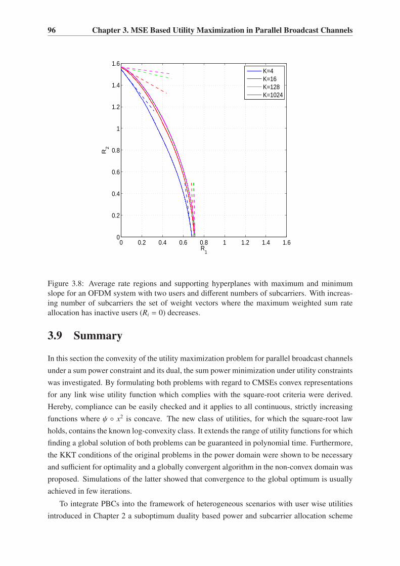
96 Chapter 3. MSE Based Utility Maximization in Parallel Broadcast Channels
0 0.2 0.4 0.6 0.8 1 1.2 1.4 1.60
0.2
0.4
0.6
0.8
1
1.2
1.4
1.6
R1
R2
K=4K=16K=128K=1024
Figure 3.8: Average rate regions and supporting hyperplanes with maximum and minimum
slope for an OFDM system with two users and different numbers of subcarriers. With increas-
ing number of subcarriers the set of weight vectors where the maximum weighted sum rate
allocation has inactive users (Ri = 0) decreases.
3.9 Summary
In this section the convexity of the utility maximization problem for parallel broadcast channels
under a sum power constraint and its dual, the sum power minimization under utility constraints
was investigated. By formulating both problems with regard to CMSEs convex representations
for any link wise utility function which complies with the square-root criteria were derived.
Hereby, compliance can be easily checked and it applies to all continuous, strictly increasing
functions where ψ ◦ x2 is concave. The new class of utilities, for which the square-root law
holds, contains the known log-convexity class. It extends the range of utility functions for which
finding a global solution of both problems can be guaranteed in polynomial time. Furthermore,
the KKT conditions of the original problems in the power domain were shown to be necessary
and sufficient for optimality and a globally convergent algorithm in the non-convex domain was
proposed. Simulations of the latter showed that convergence to the global optimum is usually
achieved in few iterations.
To integrate PBCs into the framework of heterogeneous scenarios with user wise utilities
introduced in Chapter 2 a suboptimum duality based power and subcarrier allocation scheme

3.9. Summary 97
under the constraint that at most one user can be assigned to each subcarrier was presented. It
was shown, that the corresponding assignments are globally optimal for the still non-convex
problem, if all constraints are met with equality. Nevertheless, by integrating a PBC like RAN
in a heterogeneous scenario in the context of Chapter 2, having each user active in the PBC
is likely to be required to achieve the maximum sum utility for large numbers of subcarriers.
Thus, the number of users for which an assignment to multiple RANs is required at the same
time cannot be bounded above as in heterogeneous scenarios with simplex like capacity regions.


Chapter 4
Queue Based Utility Maximization in
Heterogeneous Wireless Scenarios
Modern communication systems often incorporate queuing systems in connection with multi-
user scheduling in order to transform the quickly varying nature of the wireless channel into
diversity gains and increase the spectral efficiency. Hereby, scheduling represents a form of
time division multiplex, where the transmission resource is slotted into short intervals in time
and each interval is assigned to a subsets of users. Optimally, the slots are short enough to
follow the variations of the channel thereby enabling a dynamic adaption of the resource alloca-
tion in each slot and optimal exploitation of time diversity. To guarantee a maximum degree of
freedom for the scheduling decisions it is the the buffers’ function to have a sufficient amount
of users’ data packets in stock. In addition to the scheduling itself, flow control, which tunes
restocking of the buffers, represents a crucial factor for BE services with flexible data rates in
these systems. To allow for a reasonable performance evaluation of systems where the dynamic
resource allocation changes at high frequency an adaptation of the performance measures intro-
duced in the previous Chapters 2 and 3, where the channel was assumed to change slowly over
time, is required. The former defined notions of instantaneous or snapshot utilities lose their
relevance. In the context of scheduling the utility should reflect a user’s average performance
over a longer period of time than a single scheduling cycle. Based on this fact also channels’
probabilistic characteristics and the history of resource assignments represent crucial factors
for controlling the scheduling and flow control in each time slot and may have to be taken into
account for driving a wireless system at a desired operation point.
Although dynamic resource allocation in buffered systems in connection with scheduling
seems to be more costly than in the slowly varying RANs investigated in previous chapters,
many important results are available in the literature. Regarding queuing networks it is known
that maximum weighted sum rate scheduling over instantaneous rate regions at each time slot,
where the queue lengths represent the weights, is a throughput optimal strategy [TE92]. A
strategy is called throughput optimal if it keeps all queues stable for any vector of average
arrival rates that lies within the ergodic achievable rate region of the network. One important
99

100 Chapter 4. Queue Based Utility Maximization in Heterogeneous Wireless Scenarios
message revealed from this result is that throughput optimality can be achieved without knowing
the channel statistics and the achievable ergodic rate region. Relevant information regarding
previous resource assignments and channel realizations seem to be inherent in the buffer states.
A general formulation of throughput optimal scheduling strategies that use functions of the
buffer state as weights for the weighted sum rate maximization is derived in [ZW09].
Regarding BE services soft performance measures such as fairness gain importance. Here,
queue based maximum weighted sum rate scheduling in connection with queue based flow con-
trol is observed to come arbitrarily close to α-proportional fair allocations or maximize general
concave, strictly increasing utilities with regard to users’ average data rates [ES07], [Sto05],
[NML08]. While the former works use Lyapunov drift techniques to show convergence to the
optimum of their policies the framework of stochastic optimization theory is used in [KW04].
There, the authors show that instantaneous weighted sum rate maximization, using each user’s
mean rate, averaged over the previous time slots as inverse weights, as proposed in [Tse], leads
to proportional fair rate assignments without consideration of buffers. Previous work on static
rate regions in [LPW02] reveals that the weighted sum rate maximization employed by the
Transmission Control Protocol (TCP) Vegas in wireline networks with the window size as
weights, solves an equivalent sum utility maximization problem with the window size repre-
senting the dual parameters.
In this chapter, a heterogeneous scenario consisting of several radio access networks which
employ scheduling and which are equipped with buffers for each user are investigated. Contrary
to the slowly varying channels assumed in Chapters 2 and 3, quickly changing environments are
considered and optimum flow control, routing and scheduling policies are derived that maximize
the heterogeneous system’s sum utility for BE users with flexible QoS constraints. User wise
QoS measures with respect to average data rates serve as utility functions. It is assumed that
the instantaneous rate regions and the queue states are known, while no information on the
channel statistics and ergodic achievable rate regions is available, similar to the framework
in [ES07], [NML08]. More precisely, it is shown in Section 4.4 that the queue based algorithms
in [ES07], [NML08] are equivalent to dual stochastic subgradient procedures with constant step
size and that the queues take the role of the dual parameters. Based on this observation, which
allows to apply known results from stochastic optimization theory, a queue based algorithm
is derived which performs similarly to a subgradient algorithm with adaptable step size. The
advantages of the new algorithm in comparison to those proposed in [ES07] and [NML08] are
multifold: the adaptable step size allows to increase the algorithm’s convergence speed, which
is identified as a major drawback of queue based policies in [PEOM08]. There, the authors
suggested to maximize the instantaneous sum utility instead of using queue based approaches
to circumvent slow convergence. In addition, the average buffer lengths have to grow large for
the known queue based algorithms in order to get close to optimum assignments and thus cause
long delays. These drawbacks are overcome by the algorithms presented in this chapter.
Although virtual queue concepts are known [KS04] to reduce the length of the real equilib-

4.1. System Model 101
rium buffer states, these concepts are unable to balance user and air interface wise delays. The
equilibrium queue states are still proportional to the optimum dual parameters which depend on
the utility functions and the ergodic achievable rate regions. Thus, out-of-sequence problems
may occur in case a user’s packets are routed through different RANs. By introducing opti-
mum flow control, routing and scheduling policies that base their decisions upon functions of
the buffer states and the actual rate regions, this problem is also overcome in this chapter. The
functions constitute additional degrees of freedom that allow to control the equilibrium buffer
states individually for each user and air interface and therefore the delay while still maximizing
the system’s sum utility.
4.1 System Model
A time slotted scenario consisting of multiple wireless radio access technologies with M the
set of BSs of all RANs is considered. Hereby, each RAN is assumed to consist of a single BS
without loss of generality. Furthermore, it is assumed that all RANs have overlapping coverage
and that all users i ∈ I are able to cope with all technologies. The air interfaces are assumed
to be orthogonal to each other due to different carrier frequencies. A Heterogeneous Access
Management (HAM) unit, which is responsible for the flow control and routing of users’ pack-
ets, connects the wireline backbone network with the RANs’ BSs. Each BS m possesses one
buffer per user. The fill levels at time slot t are denoted by qm(t) = (q1,m(t), . . . qi,m(t), . . . , qI,m(t))
and storage for a vector wm(t) = (w1,m(t), . . .wi,m(t), . . . ,wI,m(t)) is provided. The vector’s en-
tries individually parameterize a function f (w, q) for each buffer and are used to decide on
resource allocation, flow control and routing decisions in Section 4.5 and 4.6. Depending on
the algorithm the parameters wi,m(t) = wi,m are either fixed or time dependent. An exemplary
heterogeneous system model is depicted in Figure 4.1 for two RATs with one BS each and
three users. Detailed properties of the scenario’s entities as well as on resource allocation, flow
control and routing are specified below:
• Resource allocation, scheduling (inside BSs):
At each time slot t BS m schedules packets with a rate ηm(t) ∈ RI+ with ηi,m = [ηm]i from
its buffers to users according to a policy φm(·):
ηm(t) = φm[ f (w1,m(t), q1,m(t)), . . . , f (wI,m(t), qI,m(t)),Cm(t)] (4.1)
The policy has access to BSs’ actual (functions of the) buffer states and can assign rates
within the actually feasible rate region Cm(t), which is assumed to be a convex set. For
resource allocation no information on the queues, weights or rate regions of RATs n ,
m ∈ M are known. Thus, each RAT is operated individually and may not be aware of
the heterogeneity of the overall scenario. This makes the scenario scalable and requires
almost no modifications of indivdial RANs if integrated in a heterogeneous system. It

102 Chapter 4. Queue Based Utility Maximization in Heterogeneous Wireless Scenarios
q1,m
qI,n
HAM
RAT m
RAT n
ηm
Cm
Packet source
w1,m wI,m
Routing
Flow control
Figure 4.1: System model of a heterogneous scenario consisting of a HAM unit and two RANs.
The HAM unit controls the users’ packet arrival rates and routes data to the indiviual BSs.
Thereby it bases its decisions on the actual (function of the) queue states and currently scheduled
rates. For scheduling, which is performed inside each BS, only information on the current buffer
states and the currently achievable rate region of the corresponding BS is available.
is also noted that no signaling information from the HAM is required, except in case an
update of the function f (·) occurs. A realization of the rate region Cm(t) depends on the
actual channel state and the RAT characteristics. Each realization is assumed to be IID
over time. The on average achievable ergodic rate regions, defined by
Cm = limT→∞
1
T
T∑
t=0
Cm(t) (4.2)
are assumed to be unknown.
• Flow control (inside the HAM unit):
At each time slot t the HAM unit requests packets with rate Rsum(t) = (R1(t), . . . ,Ri(t), . . . ,RI(t))
from the users’ packet sources through a wired link which does not represent a bottleneck
of the system. To make a flow control decision the HAM has access to f (wi,m(t), qi,m(t))
of all users and BSs and the rates which have been allocated at time slot t:
Rsum(t) = γ[ f (w1,1(t), q1,1(t)), . . . , f (wI,M(t), qI,M(t)), η1(t), . . . , ηM(t)]
Since links between the HAM unit and BSs are assumed to be wireline the amount of
signaling information that has to be reported from the BSs to the HAM unit is not regarded
a critical factor. In the oposing downlink direction where the data traffic is usually higher
because of unsymetric capacities in real world wireless networks, almost no signaling

4.2. Problem Formulation 103
information is required.
• Routing (inside the HAM unit):
The flow of packets of user i which enters the HAM unit at a rate Ri determined by the
flow control is split and routed to the queues of the individual BSs with rates Ri,m(t) and∑
m∈M Ri,m(t) = Ri(t). No extra information except the one available for the flow control
is needed to perform optimal routing decisions and no queuing of the packets inside the
HAM unit is required through instantaneous routing.
Based on the policies defined above the queues of users evolve corresponding to the following
model:
qi,m(t + 1) =[
qi,m(t) + Ri,m(t) − ηi,m(t)]
0 ∀i,m ∈ I,M (4.3)
4.2 Problem Formulation
Having introduced the system model the problem formulation is presented next. It is aimed to
find routing and flow control policies for the HAM unit and corresponding resource allocation
policies in the RANs’ BSs that maximize the sum utility of users over the unknown, ergodic
rate regions:
U∗ = max∑
i
ψ
∑
m
ηi,m
subj. to ηm ∈ Cm ∀m ∈ M(P4)
In (P4) ψ(·) is a concave, twice differentiable, strictly increasing utility function and since
Cm m ∈ M are convex the latter is a convex optimization problem that can be solved by a
multitude of algorithms such as those introduced in Chapter 2 and 3 in polynomial time in case
all Cm m ∈ M are known. However, due to the assumptions that the on average achievable
ergodic rate regions are unknown these algorithms cannot be applied. Formulating the problem
in terms of the realizations of the achievable rate regions (P4) results in
U∗ = max∑
i
ψ
∑
m
limT→∞
1
T
T∑
t=1
ηi,m(t)
subj. to ηm(t) ∈ Cm(t) ∀m ∈ M, t ≤ T
4.3 Queue Based Flow Control and Scheduling
Next, the queue based Algorithm 9 to solve problem (P4) under the requirements of the system
model is presented. This algorithm does not aim to tune the equilibrium buffer states of the
users and thus f (w, q) is set to f (wi,m(t), qi,m(t)) = qi,m(t) ∀i,m ∈ I,M. The scalar parameter

104 Chapter 4. Queue Based Utility Maximization in Heterogeneous Wireless Scenarios
Algorithm 9 Queue Based Utility Maximization
At each time slot t do
Resource Allocation:
Each BS m ∈ M allocates data rates that maximize the weighted sum rate over the rate
region’s actual realization with the buffer states as weights:
ηm(t) = arg maxηm∈Cm(t)
∑
i∈Iqi,m(t)ηi,m (4.4)
Flow control and Routing:
For each user i ∈ I packets are routed to BS m ∈ M with rate:
Ri,m(t) =s(t)
kψ′−1
(
1
kqi,mi(q)(t)
)
1m=mi(q) +
(
1 − s(t)
k
)
ηi,m(t) (4.5)
k ∈ R++ in Algorithm 9 is a positive constant which jointly controls the equilibrium buffer states
of all queues and s(t) a step size parameter. The indicator function is given by 1m=n which is
equal to one for m = n, zero for m , n, and
mi(q) = arg minm∈M
qi,m(t).
The inverse of the derivative of the utility function is denoted by ψ′−1(·) with ψ′−1(∂∂xψ(x)
)
= x.
The following result holds for Algorithm 9:
Lemma 6. Assuming that for the step size
0 ≤ s(t)
k≤ 1 ∀t ≤ T (4.6)
limt→∞
s(t)
k= 0 (4.7)
limT→∞
T∑
t=0
s(t)
k= ∞ (4.8)
limT→∞
T∑
t=0
(
s(t)
k
)2
< ∞ (4.9)
holds, then Algorithm 9 converges to the solution of problem (P4) with probability one.
Proof. The proof is a direct consequence of the derivations in Section 4.4. Equation (4.6) is
needed to guarantee non-negativity of the flow control. �
4.4 Stochastic Subgradient Interpretation
In this section the equivalence of Algorithm 9 and a dual stochastic subgradient procedure is
derived. To gain better intuition first fixed rate regions Cm(t) = Cm ∀m ∈ M are assumed and it

4.4. Stochastic Subgradient Interpretation 105
is shown that the flow control, routing and scheduling rules in Algorithm 9 maximize the dual
function of an auxiliary problem to (P4) which has the same solution. Furthermore, equivalence
of the buffers and the dual parameters follows and both evolve similarly in the direction of a
subgradient. This interpretation is then extended to time variant rate regions based on stochastic
subgradients.
Constant Rate Regions
The auxiliary problem is defined as:
max∑
i
ψ
∑
m∈MRi,m
subj. toRi,m
k≤ ηi,m
k∀i,m ∈ I,M
ηm ∈ Cm ∀m ∈ MRi,m ≥ 0 ∀i,m ∈ I,M
(P4’)
which is equivalent to (P4) for constant regions. Its dual function is given by
g(λ,σσσ) =maxR
∑
i
ψ
∑
m∈MRi,m
− 1
k
∑
m
λi,mRi,m +∑
m
σi,mRi,m
︸ ︷︷ ︸
flow control
+1
k
∑
m
maxηm∈Cm
∑
i
λi,mηi,m
︸ ︷︷ ︸
resource allocation
(4.10)
with R ∈ RI×M with [R]i,m = Ri,m and λ, σσσ ∈ RI×M+ non-negative dual parameters. A direct
consequence of duality theory is that
minλ,σσσ�0
g(λ,σσσ) (4.11)
and (P4’) have the same solution since Slater’s condition holds [Ber95a]. Furthermore, one
observes that (4.10) decouples into two maximization groups for given λ, flow control and
resource allocation: to maximize the flow control part in (4.10) over the rates the following has
to hold for a given λ+:
∑
m
Ri,m = ψ′−1
(
1
kλ+i,m − σi,m
)
∀i,m ∈ I,M. (4.12)

106 Chapter 4. Queue Based Utility Maximization in Heterogeneous Wireless Scenarios
Substituting (4.12) into the dual formulation allows to directly minimize the dual function over
σσσ, which results in setting:
σi,mi(λ+) = 0 ∀i ∈ I,mi(λ
+) = arg minm∈M
λ+i,m (4.13)
Furthermore, in case the BSs mi(λ+) are unique for all users i ∈ I, (4.12) can be solved for
Ri,m by exploiting the KKT conditions which correspond to the last constraint in (P4’): since
σi,mRi,m = 0 ∀i,m ∈ I,M must hold for any possibly optimum rate assignment and due to
non-negativity of the dual parameters σσσ � 0, λ � 0 only rate assignments
R+i,m(λ+) =
ψ′−1
(
1
kminm∈M
λ+i,m
)
if m = mi(λ+)
0 else
(4.14)
have to be considered. In case a user’s BS mi(λ+) is not unique and the set
Mi(λ+) = {m : m ∈ M,m = arg min
m∈Mλ+i,m} (4.15)
has a cardinality larger than one any rate assignment that satisfies
∑
m∈Mi(λ+)
R+i,m = ψ′−1(
1
kminm∈M
λ+i,m) (4.16)
and R+i,m = 0 ∀i,m ∈ M,I,m <Mi(λ+) maximizes the flow control part in (4.10) and complies
with the KKT conditions above.
The optimum resource allocation in (4.10) for a given λ+
η+i,m(λ+) = arg maxηm∈Cm
∑
i∈Iλ+i,mηi,m (4.17)
represents a weighted sum rate maximization which is assumed to be solvable inside the BSs
by an appropriate procedure for fixed capacity regions Cm(t) = Cm, ∀m ∈ M.
Based on the analysis above λ remains the only unknown in the dual function. To minimize
(4.11) over the latter and thus solve (P4’) an iterative algorithm based on a subgradient can be
used. A subgradient can be derived from the following observation: assuming that R+, η+ with
η ∈ RI×M with [η]i,m = ηi,m solve the inner maximization in (4.10) for a given λ+, then
g(λ) ≥ L(
R+, η+, λ)
(4.18)
= L(
R+, η+, λ+) − 1
k
∑
i∈I
∑
m∈M
(
λi,m − λ+i,m) (
R+i,m − η+i,m)

4.4. Stochastic Subgradient Interpretation 107
holds with the Lagrangian function
L(R, η, λ) =∑
i
ψ(Ri) −1
k
∑
i∈I
∑
m∈Mλi,m(Ri,m − ηi,m). (4.19)
Consequently, based on the definition in (2.20) in connection with (4.18)
1
k
(
R+ − η+) (4.20)
represents a subgradient and gives a descent direction of g(λ). Updating the dual parameters
corresponding to
λ(t + 1) =
[
λ(t) +s(t)
k
(
R+(λ(t)) − η+(λ(t)))]
0
(4.21)
is known to converge to the minimum of the dual function [Ber95a] and thus to the solution
of (4.11) and (P4’) if (4.7)-(4.9) hold for s(t)/k and if the flow control and scheduled rates are
bounded by some constants.
The update of the dual parameters (4.21) in connection with (4.14) and (4.17) form a dual
subgradient procedure that solves (P4’) for Cm(t) = Cm, ∀m ∈ M. This procedure, however,
is reproduced by Algorithm 9: by substituting the resource allocation (4.4) and flow control
(4.5) into the queuing equation (4.3) one observes that the buffers qi,m evolve similar to the dual
parameters λi,m in (4.21) and the weighted sum rate maximization in (4.4) is equal to (4.17).
Random Capacity Regions
Under the assumptions of Section 4.1 one can only evaluate η+m if the capacity regions are
fixed, and the interpretation of Algorithm 9 as dual subgradient procedure only holds under this
assumption. In case the rate regions’ realizations are random and IID, however, the following
property can be exploited: if for the subgradient at a given λ+
R+(λ+) − η+(λ+) = Et
[
R+(λ+) − η+(t, λ+)] (4.22)
holds with
η+m(t, λ+) = arg maxηm∈Cm(t)
∑
i∈Iλ+i,mηi,m, (4.23)
then one can represent
R+(λ+) − η+m(t, λ+) = R+(λ+) − η+m(λ+) + δM(t|λ+) (4.24)
as a noisy estimate of the subgradient with δM(t|λ+) being a random variable with zero mean
which complies with martingale difference noise properties [KY03]. Consequently, it follows

108 Chapter 4. Queue Based Utility Maximization in Heterogeneous Wireless Scenarios
from Theorem 2.1, Chapter 5 in [KY03] that
R+(λ+) − η+(t, λ+) (4.25)
is a stochastic subgradient of (P4’) for random capacity regions. Furthermore, the update pro-
cedure
λ(t + 1) = λ(t) +s(t)
k
(
R+(λ(t)) − η+(t, λ(t))) (4.26)
in connection with (4.23) and (4.14) converges to the optimum dual parameters
limt→∞λ(t) = λ∗ (4.27)
with probability one assuming that for the step size s(t)/k (4.7)-(4.9) hold. For the correspond-
ing flow control, routing and resource allocation
Et
[
η+i,m(t, λ∗)]
= R+i,m(
λ∗)
= η∗i,m = R∗i,m ∀i,m ∈ I,M (4.28)
follows, with (·)∗ denoting the optimum variables which also solve (P4):
∑
i
ψ
∑
m
η∗i,m
= U∗ (4.29)
Substituting the algorithm’s flow control and scheduling into the queuing equation one ob-
serves that Algorithm 9 mimics the stochastic subgradient procedure by replacing λ with q and
the proof of Lemma 6 follows directly. At the optimum the subgradient is zero so that for the
optimum buffer lengths
q∗i,m = k∂
∂xψ(x)|x=∑m∈M η∗
i,m∀i,m ∈ M (4.30)
holds.
Based on the derivations above one is now able to analyze the algorithms proposed in [ES07]
and [NML08] in the context of stochastic subgradient procedures. There, the authors proposed
algorithms that are equivalent to Algorithm 9 if s(t)/k = 1 is chosen for slightly different system
models. In [ES07] a single cell BC scenario is analyzed while in [NML08] a multihop network
is considered. In both works Lyapunov drift techniques are used to derive upper bounds on the
algorithms’ performance degradation from the global optimum in dependence of the constant
k. The latter directly influences the flow control and therefore also the equilibrium buffer states.
There it is observed that the degradation decreases with increasing k while the equilibrium
buffer lengths increase at the same time. For convergence to the global optimum the average
equilibrium buffer lengths must additionally converge to infinity ∗. The latter requirement is a
consequence of rate regions’ random nature and is explained in the following: for strictly convex
∗By interpreting the algorithms as stochastic subgradient procedures also the results on constant step size from
[KY03], Chapter 11.1.2 can be applied.

4.5. Tuning of Equilibrium Buffer States 109
ergodic rate regions global optimality of an assignment can only be achieved if the scheduling
operation is performed with the same, constant weight vector for each realization. If the buffers
represent the weights, thus, either the buffers’ lengths have to be large so that their variations,
caused by the random number of packets which leave the buffers, are small; or the flow control
must be able to instantaneously balance the buffers’ variations which are caused by the random
nature of the rate regions. For constant step sizes s(t)/k = 1 as in [ES07] and [NML08] the
former is the required to guarantee achieving the optimum. Contrary to this, the flow control
(4.5) in Algorithm 9 feeds back the actually scheduled rates for s(t)/k < 1. Thereby it balances
the variations of the buffers and for s(t)/k → 0 they stay constant independently of their lengths
and k. Thus, convergence to the global optimum can be guaranteed for Algorithm 9 also for
finite buffer lengths.
4.5 Tuning of Equilibrium Buffer States
In Section 4.4 it was observed that Algorithm 9 can be interpreted as a stochastic subgradient
algorithm with the queues resembling the dual parameters. This immediately reveals the follow-
ing disadvantages of Algorithm 9: the optimum dual parameters λ∗ and equivalently the queues
q∗ which solve (4.10) are predetermined by the average ergodic rate regions in connection with
the utility function and the scalar parameter k by (4.30). Thus, since a user’s equilibrium queue
lengths are equal in all RANs, q∗i,m = q∗i,n ∀n,m ∈ M, i ∈ I and equality of the scheduled rates
does not hold in general η∗i,m , η∗i,n ∀m , n ∈ M, i ∈ I, also the delays of a user’s packets
which are routed through different BSs may differ severely. The corresponding delays can be
calculated by Little’s Law:
di,m :=Et[qi,m(t)]
Et[ηi,m(t)]∀i,m ∈ I,M (4.31)
Different delays may result in out-of-sequence problems of a user’s packet stream. To overcome
these limitations Algorithm 10, which uses functions of the buffer state instead of pure queue
lengths as weights for the scheduling inside BSs, is derived. To guarantee its convergence to
the optimum rate assignments the algorithm is designed so that f (w, qi,m(t)) evolves exactly as
the dual parameters λi,m(t) ∀i,m ∈ I,M of the equivalent stochastic subgradient procedure
(or equivalently to qi,m(t) of Algorithm 9). Hereby, q(t) ∈ RI×M+ with [q]i,m = qi,m denotes the
buffer states obtained if Algorithm 10 (or 11) is applied and q(t) those obtained by Algorithm
9 for better readability. By parameterizing the function f (w, q) through wi,m ∀i,m ∈ I,Mthe users’ individual equilibrium buffer lengths and corresponding delays can be influenced
in each BS. No extra signaling is needed to operate Algorithm 10 once the parameters are
known inside BSs and the HAM. To guarantee equivalence of f (w, q(t)) = q(t) ∀t ≥ 0 the flow
control has to be adapted in Algorithm 10. There g(w, q) denotes the inverse of f (w, q) and
g (w, f (w, q(t))) = q(t) holds.

110 Chapter 4. Queue Based Utility Maximization in Heterogeneous Wireless Scenarios
Algorithm 10 Modified Algorithm
Resource Allocation: Each RAT m allocates data rates so that the weighted sum rate is
maximized
ηm(t) = arg maxr∈Cm(t)
∑
i∈If(
wi,m, qi,m(t))
ri,m (4.32)
Flow Control and Routing: For each user i
Ri,m(t) =
[
g
(
wi,m, f(
wi,m, qi,m(t))
+s(t)
kψ′−1
(1
kminm∈M
f(
wi,m, qi,m(t)))
− s(t)
kηi,m(t)
)
− qi,m(t) + ηi,m(t)
]
0
(4.33)
is routed to queue qi,m
Lemma 7. Assuming that f (wi,m, qi,m(t)) = wi,mqi,m(t), wi,m ≥ s(t)
k∀i,m ∈ I,M, t ≥ 0 and that
(4.7)-(4.9) hold, then Algorithm 10 converges to optimum sum utility U∗ of (P4) with probability
one, similar as Algorithm 1, but, with equilibrium buffer states:
q∗i,m =1
wi,m
q∗i,m ∀i,m ∈ I,M (4.34)
Proof. It is assumed that wi,mqi,m(t0) = qi,m(t0)∀i,m ∈ I,M holds. For better readability the
indices i,m are omitted. Then, (4.33) results in
R(t) =s(t)
kwψ′−1
(
1
kminm∈M
wq(t)
)
+
(
1 − s(t)
kw
)
η(t) (4.35)
under consideration that the flow control is non-negative for w ≥ s(t)
k. Substituting (4.35) into
the queuing equation (4.3) multiplied by w results in
wq(t + 1) = w[
q(t) + R(t) − η(t)]
0(4.36)
=
[
q(t) +s(t)
k
(
ψ′−1
(
1
kminm∈M
q(t)
)
− η(t)
)]
0
= q(t + 1)
Thus, w(q(t)) evolves exactly as q(t) for all t ≥ t0. Furthermore, the resource allocation η(t) of
Algorithms 9 and 10 are similar and thus the proof of Lemma 6 can be applied. �
Remark: Lemma 7 holds also for non-linear functions f (w, q) as long as one can guarantee
that the flow control and routing is feasible and λi,m(t) = f (wi,m, qi,m(t)) ∀i,m ∈ I,M, t ≥ 0.
For f (w, q) = wq,w <s(t)
k(indices omitted) this cannot be guaranteed since negative flow
control may be necessary to guarantee that equality of f (w, q(t)) = q(t) holds for all t ≥ 0†.
†It is noted that the conditions on f (w, q) have no connection to those in [ZW09], which guarantee throughput
optimality of scheduling policies like (4.32) in networks without flow control.

4.6. Adaptive Tuning of Queues 111
Algorithm 11 Adaptive Algorithm
Resource Allocation: Each BS m allocates data rates so that the weighted sum rate is maxi-
mized
ηm(t) = arg maxr∈Cm(t)
∑
i
wi,m(t)qi,m(t)ri,m (4.37)
Flow Control and Routing: For each user i
Ri,m(t) =
s(t)
k
(
ψ′−1(1
kminm∈M wi,m(t)qi,m(t)
) − ηi,m(t))
− sw(t)(qi,m(t) − qi,m)qi,m(t)
wi,m(t) + sw(t)(qi,m(t) − qi,m)+ ηi,m(t)
(4.38)
with sw(t) ≥ 0 chosen so that Ri,m(t) ≥ 0 and wi,m(t + 1) ≥ 0 ∀i,m ∈ I,M holds
Weight Update:
wi,m(t + 1) = wi,m(t) + sw(t)(
qi,m(t) − qi,m
)
(4.39)
One important observation in Lemma 7 is that w is not bounded above. Thus, the average
queue lengths q can be made arbitrarily small.
4.6 Adaptive Tuning of Queues
In the last section Algorithm 10 was presented which enables individual tuning of the users
equilibrium buffer states. Since the optimum q∗, or λ∗, are usually not known at the initia-
tion of an algorithm it is difficult to select wi,m for achieving convergence to a desired equi-
librium buffer length qi,m ∀i,m ∈ I,M and corresponding delay. To overcome this limita-
tion and to guarantee limt→∞ qi,m = qi,m ∀i,m ∈ I,M a second dynamic control mecha-
nism is integrated into Algorithm 10 which adaptively tunes wi,m(t) and results in Algorithm
11. In the modified procedure, sw(t) represents the step size parameter for tuning w(t) and
f (wi,m(t), qi,m(t)) = wi,m(t)qi,m(t) is chosen. Furthermore, the flow control of Algorithm 11 is
designed in a way that wi,m(t)qi,m(t) = λi,m(t) holds and λ(t) given by (4.26).
Lemma 8. Assuming that wi,m(t) ≥ s(t)
k∀ t ≥ 0 and that (4.7)-(4.9) hold, then Algorithm 11
converges to
limt→∞
∑
i
ψ
∑
m
Et[ηi,m(t)]
= U∗ with probability one. (4.40)
Furthermore, if η∗i,m > 0 ∀i,m ∈ I,M, then there exists a sequence of sw(t) for which
limt→∞
qi,m(t) = qi,m ∀i,m ∈ I,M with probability one. (4.41)
Proof. The first part of Lemma 8 follows by substituting (4.38) and (4.37) into (4.3). Then, one
obtains the update equation for the stochastic subgradient (4.26) by replacing wi,m(t)qi,m(t) with
λi,m(t) ∀i,m ∈ I,M. Together with the requirements for the step size s(t) convergence of the

112 Chapter 4. Queue Based Utility Maximization in Heterogeneous Wireless Scenarios
procedure to the global optimum follows according to Lemma 6 with probability one.
To prove the lemma’s second part the following Lyapunov function is introduced:
L(q(t)) =∑
i∈I
∑
m∈M(qi,m(t) − qi,m)2, t ≥ t0 (4.42)
Negativity of its expected drift ∆L(q(t)) = E[L(q(t + 1)) − L(q(t))] for any buffer state q(t) , q
and equality to zero for q∗ is sufficient for limt→∞ q(t) = q to hold [KY03]. By substituting
(4.37) and (4.38) into the queuing equation (4.3) and the assumption that η(t) = η∗ for t ≥ t0 the
expected drift results in
∆L(q(t)) =∑
i∈I
∑
m∈M∆q2
i,m(t)
sw(t)2
(
wi,m(t) + sw(t)∆qi,m(t))2− 2sw(t)
wi,m(t) + sw(t)∆qi,m(t)
(4.43)
with ∆qi,m(t) = qi,m(t + 1) − qi,m(t) ∀i,m ∈ I,M for t ≥ t0. It is strictly negative under the
assumption that wi,m(t) ≥ s(t)/k ∀t ≤ T and
0 ≤ sw(t) ≤ mini∈I
minm∈M
2wi,m(t). (4.44)
The requirement η∗i,m > 0 ∀i,m ∈ M ensures that any queue length can be reduced by switch-
ing off the flow control and that there always exists a feasible step size sw(t) > 0 ∀t ≥ t0
with probability one. Thus, a sequence of sw(t) which complies which limt→∞ sw(t) = 0,
limT→∞∑T
t=0 s2w(t) < ∞ and limT→∞
∑Tt=0 sw(t) = ∞ can be always found. The latter conditions
are equivalent to fulfilling the step size requirements of Theorem 2.1, Chapter 5 in [KY03],
and in connection with the negative drift guarantee convergence of limt→∞ qi,m(t) = qi,m for all
i,m ∈ I,M. This concludes the proof. �
4.7 Simulation Results
In this section the performance of Algorithms 9-11 is evaluated for a heterogeneous scenario
consisting of two colocated BSs employing different radio access technologies. Within a dis-
tance of 300-1800 meters to the BSs there are 6 users requesting packet based services with
flexible data rates. In both BSs it is assumed that only one user is scheduled per time slot. The
data rate which user i ∈ I would be assigned in BS m ∈ M on average if scheduled in each
time slot is denoted by Ri,m and depends on the RAT and the user’s distance to the BSs. They
are listed in Table 4.1. The rates correspond to those achievable in a WiMAX and HSDPA BS,
respectively and originate from [KSB+08] with units optionally in Mbit/s or in number of queue
slots emptied per time slot. For the latter to hold, it is assumed that packets with a size of 2 kbit
in sum fit into one queue slot and that scheduling intervals are 2 ms.
The data rate between the HAM unit and buffers inside BSs is limited by 100Mbit/s per link.
One major reason for the high spectral efficiency of HSDPA and WiMAX are the RANs’ pos-

4.7. Simulation Results 113
Table 4.1: Average data rates in dependence of distance for WiMAX and HSDPA
Index i=1 i=2 i=3 i=4 i=5 i=6
Distance [m] 300 600 900 1200 1500 1800
RAT 1: Ri,1 [Mbit/s] 5.70 4.80 3.00 2.22 1.32 0.72
RAT 2: Ri,2 [Mbit/s] 4.00 3.60 2.40 1.10 0.50 0.10
sibilities to exploit diversity gains originating from fast fading. In the simulations this effect is
modeled by assuming a linear relation between users’ data rates and the fast fading realizations
of the channels with respect to their average values. A realization of the rate region is given by
Cm(t) =
ηm :
∑
i∈I
ηi,m
Rfad,i,m(t)≤ 1, ηi,m ≥ 0
∀m ∈ {1, 2} (4.45)
where Rfad,i,m(t) is a random realization of an exponentially distributed variable with average Ri,m
according to (2.1). No closed form expression for Cm can be given since the regions strongly
depend on the distribution of Rm and on the number of users.
In all simulations long term proportional fair rate assignments are desired which correspond
to maximizing the following utility at time t:
U(t) =∑
i∈Ilog
1
t
t∑
τ=1
ηi,1(τ)
Mbit/s+ηi,2(τ)
Mbit/s
(4.46)
In Figure 4.2 the influences of the parameter k and the step size on the performance of Al-
gorithm 9 is evaluated. For fixed step size s(t)/k = 1, which corresponds to the algorithms
presented in [ES07] and [NML08], the tradeoff between convergence speed and close to opti-
mum operation becomes visible in the blue and red curves which represent the sum utility for
k = 1400 and k = 70 over time, respectively. While a faster increase of U(t) at low t and quick
convergence is obtained for k = 70 it comes at the cost of a severe degradation of the sum utility
compared to the one achieved for k = 1400 and constant step size. Algorithm 9 in connection
with flexible step size selection s(t) = k/t0.3 and k = 70 combines achieving the maximum sum
utility and fast convergence. This is reflected by the green curve in the figure. The influence of
k and s(t) on the evolution of the queues and delays is shown in Figure 4.3 and 4.4. The delay
is defined in dependence of the scheduled rates’ moving average:
di,m(t) =qi,m(t)
1T
∑τ=T−1τ=0 ηi,m(T − τ)
∀i,m ∈ I,M, t ≥ T, T = 100.
As one could expect, the simulation with k = 1400 results in 20 times higher equilibrium queue
lengths and also delays compared to the simulations with k = 70. The large variations of the
queue lengths compared to their average values are responsible for the performance degradation
of the constant step size simulation with k = 70 . These directly influence the scheduling

114 Chapter 4. Queue Based Utility Maximization in Heterogeneous Wireless Scenarios
0.5 1 1.5 2 2.5 3 3.5 4 4.5 5
x 104
1.5
2
2.5
3
3.5
t [scheduling slots]
U(t
)
Alg 9 k=1400 s(t)/k=1
Alg 9 k=70 s(t)/k=1
Alg 9, 10, 11 k=70 s(t)=k/t0.3
Alg 9 delay k=70 s(t)=k/t0.3
Alg 9 separate k=70 s(t)=k/t0.3
Figure 4.2: Influence of step size, k, delay in the flow control and separated user assignments
on the evolution of the sum utility for Algorithm 9, 10 and 11. Utilizing a decreasing step size
s(t)/k = t−0.3 in Algorithms 9, 10 and 11 outperform the fixed step size s(t)/k = 1 operation
of Algorithm 9 in terms of sum utility and convergence speed. In case the information for
calculating the flow control is outdated or under the constraint that users can be assigned to at
most one air interface the performance degrades.
process and prevent the queues from converging to the optimum weights even on average. In
the simulation with decreasing step size the variations are strongly damped and convergence to
the optimum weights is achieved. Here, the variations of the queue which are caused by the
scheduling are compensated through the flow control.
Figure 4.2 shows the evolution of the sum utility for two additional simulations. The green
curve corresponds to Algorithm 9 with k = 70, s(t)/k = t−0.3 and the assumption that only
outdated information on the scheduled data rates is available for the flow control. For this
simulation the flow control is calculated by
Ri,m(t) =s(t)
kψ′−1
(
1
kqi,m∗
i(t)(t)
)
1m=m∗i(t) +
(
1 − s(t)
k
)
ηi,m(t − 1)
instead of using (4.5) in Algorithm 9. The delay leads to a performance degradation, which is
smaller than the loss at fixed step size operation and k = 70, however‡.
‡Analyzing the influence of the delay on the algorithm’s performance and on global stability analytically is
difficult [LS04], specifically for random rate regions. It requires solving a set of delay differential equations. Thus,
often linearization of the equations is used in the literature, which, however, guarantees only local stability in the

4.7. Simulation Results 115
1 2 3 4 5
x 104
0
500
1000
1500
2000
t [scheduling slots]
q 2
k=1400, s(t)/k=1
1 2 3 4 5
x 104
0
20
40
60
80
100
120
140
160
t [scheduling slots]
q 2
k=70, s(t)/k=1
1 2 3 4 5
x 104
0
20
40
60
80
100
120
t [scheduling slots]
q 2
k=70, s(t)/k=t−0.3
User 1
User 2
User 3
User 4
User 5
User 6
Figure 4.3: Influence of step size s(t) and k on the evolution of queues of RAT 2 of Algorithm
9. Small step sizes reduce the ratio of queues’ variance and equilibrium length.
1 2 3 4 5
x 104
0
2000
4000
6000
8000
10000
12000
t [scheduling slots]
d 2 [slo
t dur
atio
n]
k=1400, s(t)/k=1
1 2 3 4 5
x 104
0
100
200
300
400
500
600
700
800
900
1000
t [scheduling slots]
d 2 [slo
t dur
atio
n]
k=70, s(t)/k=1
1 2 3 4 5
x 104
0
100
200
300
400
500
600
t [scheduling slots]
d 2 [slo
t dur
atio
n]
k=70, s(t)/k=t−0.3
Figure 4.4: Influence of step size s(t) and k on users’ delays in RAT 2 for Algorithm 9 (legend
as in Figure 4.3).
The magenta curve corresponds to the performance of Algorithm 9 with k = 70, s(t)/k =
t−0.3 and the additional constraint that each user is assigned to at most one air-interface. Assign-
ing the nearest 4 users to RAT 1 and the remaining 2 to RAT 2 maximizes the sum utility in the
investigated scenario in this case, but at large performance losses compared to having all users
active in both RATs and therefore full diversity. An analytical analysis of the performance gain
of possibly having all users active in all RATs compared to restricting each user to one tech-
nology requires knowledge about the underlying rate regions. Since the latter strongly depend
on the number of users, the RAN characteristics and fading distributions no general results are
presented here.
The performance of Algorithm 10 with k = 70 and s(t)/k = t−0.3 for the same scenario
vicinity of the optimum solution [ZWL07].

116 Chapter 4. Queue Based Utility Maximization in Heterogeneous Wireless Scenarios
1 2 3 4 5
x 104
0
5
10
15
20
25
30
35
40
0 1 2 3 4 5
x 104
0
20
40
60
80
100
120
1 2 3 4 5
x 104
0
10
20
30
40
50
60
70
80
90
100
t [scheduling slots]t [scheduling slots]t [scheduling slots]
q1
wq
1
d1
[sch
edu
lin
gsl
ots
]
1 2 3 4 5
x 104
0
5
10
15
20
25
30
35
40
1 2 3 4 5
x 104
0
20
40
60
80
100
120
1 2 3 4 5
x 104
0
10
20
30
40
50
60
70
80
90
100
t [scheduling slots]t [scheduling slots]t [scheduling slots]
q2
wq
2
d2
[sch
edu
lin
gsl
ots
]
Figure 4.5: Influence of f (w, q(t)) = wq(t) on the evolution of queues, weighted queues and
delays of RAT 1 and 2 for Algorithm 10 with s(t)/k = t−0.3, k = 70. While the weighted queues
evolve similarly to the ones if Algorithm 9 is applied the real buffers and delays scale with the
inverse of the weights w1 = (1.00, 1.19, 1.90, 2.57, 4.32, 7.92), w2 = (1, 1, 1, 100, 100, 100).
(legend as in Figure 4.3)
and f (wi,m, qi,m(t)) = wi,mqi,m(t) ∀i,m ∈ I,M is shown in Figure 4.5 for the first and second
air interface, respectively. Here, the inverse of each user’s averaged sum rate 1/(Ri,1 + Ri,2)
normalized so that the smallest entry is equal to one serve as weight vector for the first BS in
the simulations w1 = (1.00, 1.19, 1.90, 2.57, 4.32, 7.92). The latter are expected to balance the
users equilibrium queue lengths in this BS since proportional fair assignments result in optimum
dual parameters which are proportional to the inverse of the average rate. For the second BS
w2 = (1, 1, 1, 100, 100, 100) is used which reduces the equilibrium buffer states of users 4-6
to one percent of the values obtained in Figure 4.3 with Algorithm 9. As can be observed in
Figure 4.5 the weighted queue lengths f (wi,2, qi,2(t)) = wqi,2(t) of BS 2 evolve similarly to the
queues in Figure 4.3, the real buffers and the delays are reduced by a factor w, however.
Figure 4.6 shows the evolution of the real and weighted queues as well as the delays if
Algorithm 11 is applied. Again k = 70, s(t)/k = t−0.3 is used and delays of di,m = 5 schedul-

4.8. Summary 117
1 2 3 4 5
x 104
0
2
4
6
8
10
12
14
16
18
20
0 1 2 3 4 5
x 104
0
20
40
60
80
100
120
1 2 3 4 5
x 104
0
2
4
6
8
10
12
14
16
18
20
t [scheduling slots]t [scheduling slots]t [scheduling slots]
q1
wq
1
d1
[sch
edu
lin
gsl
ots
]
1 2 3 4 5
x 104
0
2
4
6
8
10
12
14
16
18
20
1 2 3 4 5
x 104
0
20
40
60
80
100
120
1 2 3 4 5
x 104
0
2
4
6
8
10
12
14
16
18
20
t [scheduling slots]t [scheduling slots]t [scheduling slots]
q2
wq
2
d2
[sch
edu
lin
gsl
ots
]
Figure 4.6: Influence of adaptive weight control in Algorithm 11 with f (w(t), q(t)) = w(t)q(t),
s(t)/k = t−0.3, sw(t) = 0.03t−0.1, k = 70 and desired delays di,m(t) = 5 time slots ∀i,m ∈ I,M.
(legend as in Figure 4.3)
ing slots equivalent to 10ms are desired for all users in both BSs. To integrate the required
delays in Algorithm 11 desired equilibrium buffers q corresponding to sliding averages with
qi,m(t) = di,m1T
∑T−1τ=0 ηi,m(t − τ), T = 100,∀i,m ∈ I,M are used. The step size sw(t) is cho-
sen corresponding to sw(t) = 0.03t−0.1. As can be observed in the figure, the weighted queues
evolve similarly to the real and weighted ones obtained by Algorithm 9 and 10 in Figures 4.3
and 4.5, respectively. The delays, however, converge to the desired values di,m = 5∀i,m ∈ I,Malthough this corresponds to different equilibrium buffer states in the BSs.
4.8 Summary
In this chapter decentralized algorithms for the utility maximization in heterogeneous queuing
scenarios in quickly changing environments were proposed. These algorithms, consisting of
flow control, routing and resource allocation thereby base their decisions upon functions of the

118 Chapter 4. Queue Based Utility Maximization in Heterogeneous Wireless Scenarios
buffer states and instantaneous rate regions and converge to rate assignments that correspond to
the optimum sum utilities over the unknown, ergodic rate regions.
Contrary to known algorithms, which are identified as stochastic subgradient procedures
with constant step size in Section 4.4, the proposed Algorithms 9, 10 and 11 are similar to
stochastic subgradient procedures with tunable step size. This proves advantageous with regard
to the convergence speed and the delay in the simulations: by choosing small step sizes the
equilibrium buffer lengths and thus the delays can be jointly reduced almost arbitrarily without
any performance loss.
By using functions of the buffer states for flow control, routing and resource allocation,
Algorithms 10 and 11 are able to tune users’ individual delays in all BSs. Thereby they prevent
out-of-sequence problems of users’ packet flows.

Chapter 5
Conclusions and Outlook
5.1 Conclusions
In this thesis the resource allocation in wireless scenarios which consisted of several radio ac-
cess networks with overlapping coverage and where operators have the freedom to assign users
to a technology of their choice was analyzed. Emphasis was put on the design of algorithmic
solutions that consider practical limitations of real world scenarios. Where global optimality of
the procedures could not be proved, bounds on the optimum solution were provided to allow
for expedient performance evaluations and comparisons.
The first part of the thesis was dedicated to multi-system scenarios in slowly changing en-
vironments. By exploiting the fact that some air interfaces support certain service classes more
efficiently than others - a characteristic resulting e.g. from technology dependent coding and
modulation schemes - an algorithmic concept which maximizes the total number of assignable
users was proposed. Rewriting the underlying optimization problem as a max-min formulation
constituted the key property for the derivation of an intuitive and quickly converging algorithm.
In the analyzed model users had fixed QoS requirements and the feasible rate regions of individ-
ual BS were assumed to be known. Gains of approximately 15% could be obtained compared
to a simple load balancing strategy.
Having used the air interfaces’ service dependent suitability in the previous analysis, users’
individual channel gains were then also considered. The latter provided an additional source of
diversity since air interfaces are subject to e.g. different propagation losses based on different
carrier frequencies and diverse sensitivity to interference. A cost model was introduced which
comprisesd all relevant air interface and service specific characteristics in one scalar parame-
ter per user and BS. Then, an algorithm was derived for maximizing the weighted number of
assignable users in a heterogeneous multi-cell UMTS GSM/EDGE scenario. Due to the practi-
cally motivated constraint that users cannot be assigned to multiple radio access networks at the
same time an approximate algorithm was derived using continuous relaxation. This provably
resulted in an assignment with at most M users less than at the global optimum. The algorithm
119

120 Chapter 5. Conclusions and Outlook
was then adapted to the probabilistic nature of service requests, channels and users’ mobility
by a more robust design. The latter approached the vicinity of the optimum by a subgradient
directed vertex search and increased the number of supportable users by approximately 20%
even in single service setups.
While the former analysis was restricted to services with fixed QoS constraints BE users
were integrated by introducing a utility concept. It represents a framework to flexibly measure
the quality of an assignment with regard to fairness, system throughput, user priorities or com-
binations thereof. Extending the ideas of the cost based concept, an optimum cell selection and
resource allocation rule which maximized the BE users’ sum utility and guaranteed service to
the users with fixed QoS constraints at the same time was derived. Although the corresponding
algorithm operated in a completely distributed way it still required a non negligible amount
of signaling between users and BSs. Thus, an adaptation of the procedure which reduced the
required signaling to a single reciprocal information exchange between the BSs and a new user
at its service setup request was proposed. The reduction of the signaling effort came at the cost
of the algorithms’ optimality which could not be guaranteed anymore. However, close to the
optimum operation was observed in simulations by comparing it to an upper bound in a hetero-
geneous UMTS GSM/EDGE system. The scenario’s utility and throughput increased by up to
30% compared to a load balancing strategy.
To further extend the previously introduced air interface models where either the bandwidth
or the power represented the assignable resource, parallel broadcast channels were investigated.
They allow for both, power allocation and subcarrier selection and serve as general model
for wireless systems like OFDM. Using a complementary mean square error representation
the square root law was derived. It holds for all utility functions whose concatenations with
f (x) = x2 are concave and guarantees the existence of a convex representation of the utility
maximization problem and the sum power minimization with regard to CMSEs. The new class
thereby represents an extension of the log-convex utility class. Furthermore, an algorithm in the
non-convex domain of powers was proposed and its convergence to the global optimum proven.
OFDM like systems were then integrated into the previously analyzed heterogeneous scenar-
ios and a suboptimum assignment strategy proposed which restricted the number of assignable
users to one on each subcarrier. Contrary to pure UMTS GSM/EDGE scenarios, close to opti-
mality of assigning each user to a single cell was lost in setups comprising all three radio access
technologies. More precisely, the property that for optimum assignments all users are likely to
be active in the OFDM system was shown.
The last part of the thesis covered the utility maximization in heterogeneous scenarios in
quickly changing environments where BSs were equipped with queues. There, it was assumed
that the achievable rate regions represented random realizations of an underlying probabilistic
channel model and it was aimed to maximize an average utility metric over time. An algo-
rithmic framework whose information was limited to queue states and the actual realization of
the rate regions was derived. The latter was shown to be equivalent to a stochastic subgradient

5.1. Conclusions 121
procedure with flexible step size and with buffers representing the dual parameters of the under-
lying optimization problem. The ability to adapt the step size proved advantageous with regard
to known buffer based concepts from the literature: it resulted in faster convergence speed,
lower delays and the fact that the global optimum could be attained for finite equilibrium buffer
lengths. The concept was then extended to allow for individual tuning of user’s delays and thus
circumventing out-of-sequence problems, which may occur in case a user’s packets are routed
to different BSs and subject to different delays.
Summarizing the results three main questions were answered in this thesis:
Why ... should air interface selection improve a heterogeneous system’s performance?
• It allows to balance air interface loads in case of asymmetric request situations or network
capacities.
• Intelligent air interface selection is able to exploit the fact that the efficiency to support
users strongly depends on the service class as well as channel characteristics and differs
between technologies. Thus, the heterogeneous system’s spectral can be increased.
• In quickly changing environments, where a user’s performance depends on random chan-
nel realizations, having the choice between multiple sources increases diversity, even if
the average efficiencies are equal for users.
How... can air interface diversity be exploited and what do optimum assignments look like?
• To maximize the supportable number of users or a parameterizable system utility (approx-
imately) convex problem reparameterizations can often be found. They allow to design
decentralized algorithms adapted to the architecture of the underlying radio networks and
the over time varying request situations.
• In air interfaces such as GSM/EDGE and UMTS simplex like rate regions result in opti-
mal allocations where almost all users are assigned to at most one air interface. In these
scenarios, the air interface selection reduces to service and air interface specific SINR
thresholds, which depend on the system configuration and the desired optimization met-
ric.
• In heterogeneous systems, where the underlying technologies employ scheduling, buffer
based flow control and scheduling policies can be designed which learn unknown ergodic
rate regions and perform similar to stochastic subgradient procedures with adaptable step
size.
Which... gains can be expected?
• All proposed algorithms increased the heterogeneous systems’ performances by up to
30% compared to simple load balancing strategies. For most assignments either optimal-
ity could be proven or bounds to the optimum solution were provided.

122 Chapter 5. Conclusions and Outlook
5.2 Outlook
Although this thesis provided insights into the structure and algorithms for the optimum air
interface selection and resource allocation the following research topics are of interest:
• Which impact does the requirement of assigning each user to at most one technology
at a time have on the system performance? This question was answered for simplex
like rate regions in the thesis. Analyzing this for general convex regions will require to
investigate the regions’ shapes and curvatures which depend on the channel distributions
and numbers of users.
• In queuing systems zero variance of the buffers is required to maximize the sum utility by
buffer based scheduling policies if the rate regions are strictly convex. It was shown that
the variance of the buffers’ fluctuation can be reduced by considering actually scheduled
rates in the flow control. In the proposed algorithms the influence of the scheduled rates
on the flow control was tuned by the step size. In real world scenarios only delayed
information on the scheduled rates may be available for flow control thereby prohibiting
elimination of the variance. Although simulations with delayed information still showed
considerable utility gains compared to known queue based strategies, the optimum step
size which minimizes the buffers’ variance is still unknown. Its calculation will require
solving non-linear delay differential equations.

Acronyms
3GPP Third Generation Partnership Project
APX Approximable
BC Broadcast
BE Best Effort
BS Base Station
CDF Cumulative Density Function
CDMA Code Division Multiple Access
CMSE Complementary Mean Square Error
DFT Discrete Fourier Transform
EDGE Enhanced Data Rates for GSM Evolution
ETSI European Telecommunications Standards Institute
FDMA Frequency Division Multiple Access
GAP General Assignment Problem
GSM Global System for Mobile Communications
HAM Heterogeneous Access Management
HIA Heuristically Improved Algorithm
HSDPA High Speed Downlink Packet Access
IID Independent and Identically Distributed
ISHO Inter-system Hand-over
KKT Karush-Kuhn-Tucker
123

124 Chapter 5. Conclusions and Outlook
LTE Long Term Evolution
MAC Multiple Access Channel
MIMO Multiple Input Multiple Output
MKP Multiple Knapsack Problem
MMSE Minimum Mean Square Error
MRM Multiple Radio Management
MRRM Multiple Radio Resource Management
MSE Mean Square Error
NP Non Polynomial
OFDM Orthogonal Frequency Division Multiplex
PBC Parallel Broadcast Channel
PDF Probability Density Function
QoS Quality of Service
RAN Radio Access Network
RAT Radio Access Technology
SINR Signal to Interference and Noise Ratio
TCP Transmission Control Protocol
TDMA Time Division Multiple Access
TIA Telecommunication Industry Association
UMTS Universal Mobile Telecommunications System
VoIP Voice over Internet Protocol
WLAN Wireless Local Area Network
WiMAX Worldwide Interoperability for Microwave Access

Publications
[1] I. Blau and G. Wunder. Optimal service allocation in multi-system scenarios with lin-
ear subsystem capacity regions. In The 9th Symposium on Wireless Personal Multimedia
Communications (WPMC ’06), San Diego, USA, 17th-20th September 2006.
[2] I. Blau and G. Wunder. User allocation in multi-system, multi-service scenarios: Upper
and lower performance bound of polynomial time assignment algorithms. In 41st Confer-
ence on Information Sciences and Systems (CISS ’07), Baltimore, USA, March 2007.
[3] I. Blau, G. Wunder, I. Karla, and R. Siegle. Cost based heterogeneous access management
in multi-service, multi-system scenarios. In Proc. IEEE 18th International Symposium on
Personal, Indoor and Mobile Radio Communications (PIMRC ’07), pages 1–5, 3–7 Sept.
2007.
[4] I. Blau, G. Wunder, I. Karla, and R. Sigle. Cost optimization MRRM algorithm procedure
for several service classes. European Patent 08F49485-HHI. (pending).
[5] I. Blau, G. Wunder, I. Karla, and R. Sigle. Dynamical utility based radio resource assign-
ment algorithm. European Patent 08F49460-HHI. (pending).
[6] I. Blau, G. Wunder, I. Karla, and R. Sigle. Resource allocation method and apparatus
thereof. U.S. Patenet 803562. (pending).
[7] I. Blau, G. Wunder, I. Karla, and R. Sigle. Resource cost considering radio access selec-
tion algorithm based on the location of mobile users. European Patent 08F49460-HHI.
(pending).
[8] I. Blau, G. Wunder, I. Karla, and R. Sigle. Decentralized utility maximization in hetero-
geneous multi-cell scenarios. In Proc. IEEE 19th International Symposium on Personal,
Indoor and Mobile Radio Communications (PIMRC ’08), Cannes, France, 2008.
[9] I. Blau, G. Wunder, I. Karla, and R. Sigle. Decentralized utility maximization in het-
erogeneous multi-cell scenarios with interference limited and orthogonal air-interaces.
EURASIP Journal on Wireless Communications and Networking, 2009, 2009. Article
ID 104548.
125

126 PUBLICATIONS
[10] I. Blau, G. Wunder, and T. Michel. Utility optimization based on MSE for parallel broad-
cast channels: The square root law. Wireless Personal Communications, 2009.
[11] G. Wunder, I. Blau, and T. Michel. Utility optimization based on MSE for parallel broad-
cast channels: The square root law. In 45th Annual Allerton Conference on Communica-
tion, Control, and Computing, Urbana, USA, 2007.

Bibliography
[3GP08] 3GPP system architecture evolution: Report on technical options and conclusions
(release 7). Technical Report TR 23.882, Third Generation Partnership Project,
2008.
[Agi99] Pascal Agin. Summary of UTRA/FDDD link-level performance results. Technical
Report REF:TD/SYT/pag/740.99, Version 1.0, Alcatel Internal report, 1999.
[BBK05] F. Baccelli, B. Blaszczyszyn, and M.K. Karray. Blocking rates in large CDMA
networks via a spatial erlang formula. Technical report, HAL - CCSD, Unite de
recherche INRIA Rocquencourt, 2005.
[Ber95a] D. P. Bertsekas. Nonlinear Programming. Athena Scientific, Belmont, Mas-
sachusetts, 2rd. edition, 1995.
[Ber95b] Dimitri P Bertsekas. Dynamic Programming and Optimal Control, volume I.
Athena Scientific, Massatchusetts, 1995.
[BK07] B. Blaszczyszyn and M. K. Karray. Performance evaluation of scalable conges-
tion control schemes for elastic traffic in cellular networks with power control. In
Proc. INFOCOM 2007. 26th IEEE International Conference on Computer Com-
munications, pages 170–178, 2007.
[Boy06] Stephen Boyd. Lecture Notes on EE364b Convex Optimization II. Stanford Uni-
versity, 2006.
[BPH06] S. Borst, A. Proutiere, and N. Hegde. Capacity of wireless data networks with
intra- and inter-cell mobility. In Proc. 25th IEEE International Conference on
Computer Communications INFOCOM 2006, pages 1–12, April 2006.
[BSK07] I. Blau, R. Sigle, and I. Karla. MRRM algorithms for packet switched traffic based
on utility maximization. Internal report STU/RBN/T/07/0026, Alcatel Lucent,
2007.
[BV04] S. Boyd and L. Vandenberghe. Convex Optimization. Cambridge University Press,
2004.
127

128 BIBLIOGRAPHY
[BW09] J. Buhler and G. Wunder. An optimization framework for heterogeneous access
management. In Proc. IEEE Wireless Communications and Networking Confer-
ence (WCNC ’09), Budapest, April 2009.
[BWS04] H. Boche, M. Wiczanowski, and S. Stanczak. Characterization of optimal resource
allocation in cellular networks. In Proc. IEEE 5th Workshop on Signal Processing
Advances in Wireless Communications, pages 454–458, 2004.
[BWS07] H. Boche, M. Wiczanowski, and S. Stanczak. On optimal resource allocation in
cellular networks with best-effort traffic. IEEE Transactions on Wireless Commu-
nications, 2007. revised.
[Car78] A. Carleial. Interference channels. Information Theory, IEEE Transactions on,
24(1):60–70, Jan 1978.
[CC06] B. Chen and M. Chan. Resource management in heterogenous wireless networks
with overlapping coverage. In First International Conference on Communication
System Software and Middleware (Commsware ’06), 2006.
[Cha66] R. W. Chang. Synthesis of band-limited orthogonal signals for multi-channel data
transmission. Bell System Technical Journal, 46:1775–1796, 1966.
[Chi05a] M. Chiang. Balancing transport and physical layers in wireless multihop networks:
Jointly optimal congestion control and power control. IEEE Journal on Selected
Areas in Communications, 23(1), January 2005.
[Chi05b] M. Chiang. Geometric Programming for Communication Systems. now Publishing
Inc., 2005.
[Cos83] M. Costa. Writing on dirty paper (corresp.). Information Theory, IEEE Transac-
tions on, 29(3):439–441, May 1983.
[Cov72] T. M. Cover. Broadcast channels. IEEE Transactions on Information Theory,
18(1):2–14, 1972.
[CRdV06] J.K. Chen, T.S. Rappaport, and G. de Veciana. Iterative water-filling for load-
balancing in wireless lan or microcellular networks. In Proc. VTC 2006-Spring
Vehicular Technology Conference IEEE 63rd, volume 1, pages 117–121, 2006.
[CT91] T. M. Cover and J. Thomas. Elements of Information Theory. John Wiley, 1991.
[CTJLa06] M. Codreanu, A. Tolli, M. Juntti, and M. Latva-aho. Weighted sum MSE mini-
mization for MIMO broadcast channel. In Proc. IEEE 17th International Sympo-
sium on Personal, Indoor and Mobile Radio Communications (PIMRC ’06), pages
1–6, 11–14 Sept. 2006.

BIBLIOGRAPHY 129
[ES07] A. Eryilmaz and R. Srikant. Fair resource allocation in wireless networks using
queue-length-based scheduling and congestion control. IEEE/ACM Trans. Net-
working, 15(6):1333–1344, Dec. 2007.
[ETS99] Radio network planning aspects. Technical Report TR 101 362 V8.3.0 (GSM
03.30 version 8.3.0 Release 1999), European Telecommunications Standards In-
stitute, 1999.
[ETS06] Digital cellular telecommunications system (phase 2+); universal mobile telecom-
munications system (UMTS); vocabulary for 3GPP specifications. Technical Re-
port TR 121 905 V7.2.0, European Telecommunications Standards Institute, 2006.
[ETW07] R. Etkin, D. N. C. Tse, and H. Wang. Gaussian interference channel capacity
to within one bit. http://www.citebase.org/abstract?id=oai:arXiv.org:cs/0702045,
2007.
[Fel68] W. Feller. An Introduction to Probability Theory and Its Applications, Volume 1.
Wiley, January 1968.
[FGMS06] L. Fleischer, M.X. Goemans, V.S. Mirrokni, and M. Sviridenko. Tight approxi-
mation algorithms for maximum general assignment problems. In Proceedings of
the 17th ACM-SIAM Symposium on Discrete Algorithms, 2006.
[FL07] A. Farbod and B. Liang. Efficient structured policies for admission control in
heterogeneous wireless networks. Mob. Netw. Appl., 12(5):309–323, 2007.
[FR] R. M Freund and C. Roos. The ellipsoid method.
www.isa.ewi.tudelft.nl/∼roos/courses/wi485/ellips.pdf.
[FT91] D. Fudenberg and J. Tirole. Game Theory. MIT Press, October 1991.
[FZ05] A. Furuskar and J. Zander. Multiservice allocation for multiaccess wireless sys-
tems. IEEE Transactions on Wireless Communications, 4(1), January 2005.
[Gol05] A. Goldsmith. Wireless Communications. Cambridge University Press, New York,
NY, USA, 2005.
[HBH06] J. Huang, R. Berry, and M. Honig. Distributed interference compenzation for
wireless networks. IEEE Journal on Selected Areas in Communications, 24(5),
May 2006.
[HEBJ08] S. Horrich, S.E. Elayoubi, and S. Ben Jemaa. A game-theoretic model for radio
resource management in a cooperative WIMAX/HSDPA network. In Proc. IEEE
International Conference on Communications (ICC ’08), pages 2592–2596, 19–
23 May 2008.

130 BIBLIOGRAPHY
[HH75] D. Hughes-Hartogs. The capacity of the degraded spectral Gaussian broadcast
channel. PhD thesis, Inform. Syst. Lab., Stanford Univ. Stanford, CA, 1975.
[Hil05] M. Hildebrand. Optimized Network Accecss in Heterogeneous Wireless Networks.
PhD thesis, Universitat Kassel, 2005.
[HJ08] R. Hunger and M. Joham. On the convexity of the MSE region of single-antenna
users. In Proc. IEEE Global Telecommunications Conference IEEE GLOBECOM
2008, pages 1–5, Nov. 30 2008–Dec. 4 2008.
[HK06] L. Hanzo and T. Keller. OFDM and MC-CDMA. John Wiley, 2006.
[HPZ05] C. Ho, F. Pingyi, and C. Zhigang. A utility-based network selection scheme for
multiple services in heterogeneous networks. In Proc. International Conference
on Wireless Networks, Communications and Mobile Computing, volume 2, pages
1175–1180 vol.2, 2005.
[HT93] R. Horst and H. Tuy. Global Optimization. Springer, 2., rev. ed edition, 1993.
[JB03] E. Jorswieck and H. Boche. Transmission strategies for the MIMO MAC with
MMSE receiver: average MSE optimization and achievable individual MSE re-
gion. IEEE Trans. on Signal Processing, 51(11):2872–2881, November 2003.
special issue on MIMO wireless communications.
[JMO03] J. Jalden, C. Martin, and B. Ottersten. Semidefinte programming for detection
in linear systems - optimality conditions and space-time decoding. In Acoustics,
Speech, and Signal Processing, 2003.
[KPP04] H. Kellerer, U. Pferschy, and D. Pisinger. Knapsack Problems. Springer, Berlin,
Germany, 2004.
[KS04] S. S. Kunniyur and R. Srikant. An adaptive virtual queue (AVQ) algorithm for
active queue management. IEEE/ACM Trans. Networking, 12(2):286–299, 2004.
[KSB+08] I. Karla, R. Sigle, I. Blau, U. Bergemann, and C. Reinke. MRRM simulator spec-
ification, version 2.8. Technical report, Alcatel Lucent, 2008.
[KW04] H. Kushner and P.A. Whiting. Convergence of proportional-fair sharing algo-
rithms under general conditions. IEEE Trans. Wireless Commun., 3(4):1250–1259,
July 2004.
[KY03] H. Kushner and G. Yin. Stochastic approximation and recursive algorithms and
applications. Springer, 2 edition, 2003.

BIBLIOGRAPHY 131
[LG01] L. Li and A. Goldsmith. Capacity and optimal resource allocation for fading
broadcast channels .i. ergodic capacity. IEEE Trans. Inform. Theory, 47(3):1083–
1102, March 2001.
[LJ06] J. Lee and N. Jindal. Symmetric capacity of MIMO downlink channels. In Proc.
IEEE International Symposium on Information Theory (ISIT ’06), pages 1031–
1035, 2006.
[LPW02] S. H. Low, L. Peterson, and L. Wang. Understanding TCP Vegas: a duality model.
J. ACM, 49(2):207–235, 2002.
[LS04] S. H. Low and R. Srikant. A mathematical framework for designing a low-loss,
low-delay internet. Networks and Spatial Economics, 4(1):75–101, March 2004.
[LTE08] UTRA-UTRAN long term evolution (LTE) and 3GPP system architecture evolu-
tion (SAE). Technical report, Third Generation Partnership Project, 2008.
[MW00] J. Mo and J. Walrand. Fair end-to-end window-based congestion control.
IEEE/ACM Trans. on Networking, 8(5):556–567, 2000.
[Net] Technical Specification Group Radio Access Networks. Improvement of RRM
across RNS and RNS/BSS (release 5). Technical Report TR 25.881 V5.0.0, Third
Generation Partnership Project.
[NML08] M. J. Neely, E. Modiano, and Chih-Ping Li. Fairness and optimal stochastic con-
trol for heterogeneous networks. IEEE/ACM Trans. Networking, 16(2):396–409,
April 2008.
[NP99] R.Van Nee and R. Prasad. OFDM for Wireless Multimedia Communications.
Artech House, Incorporated, 1999.
[OY07] C. Oh and A. Yener. Downlink throughput maximization for interference lim-
ited multiuser systems: TDMA versus CDMA. IEEE Trans. Wireless Commun.,
6(7):2454–2463, July 2007.
[Pal05] D. P. Palomar. Convex primal decomposition for multicarrier linear MIMO
transceivers. IEEE Trans. Signal Processing, 53(12):4661–4674, Dec. 2005.
[PC06] D. P. Palomar and M. Chiang. A tutorial on decomposition methods for network
utility maximization. IEEE J. Select. Areas Commun., 24(8):1439–1451, 2006.
[PDJMT04] A. Pillekeit, F. Derakhshan, E. Jugl, and A. Mitschele-Thiel. Force-based load bal-
ancing in co-located UMTS/GSM networks. In Vehicular Technology Conference
IEEE, 2004.

132 BIBLIOGRAPHY
[PDKS06] G. Piao, K. David, I. Karla, and R. Sigle. Performance of distributed MxRRM. In
Personal, Indoor and Mobile Radio Communications (PIMRC’06), 2006.
[PEOM08] A. ParandehGheibi, A. Eryilmaz, A. Ozdaglar, and M. Medard. On resource al-
location in fading multiple access channels - an efficient approximate projection
approach. Technical report, arXiv:0810.1234v1 [cs.IT], submitted to IEEE Trans-
actions on Information Theory, 2008.
[PM02] K. I. Pedersen and P.E. Mogensen. The downlink orthogonality factors influence
on wcdma system performance. In Vehicular Technology Conference, 2002. Pro-
ceedings. VTC 2002-Fall. 2002 IEEE 56th, volume 4, pages 2061–2065 vol.4,
2002.
[PRSA06] J. Perez-Romero, O. Salient, and R. Agusti. Enhanced radio access technology
selection exploiting path loss information. In Proc. IEEE 17th International Sym-
posium on Personal, Indoor and Mobile Radio Communications (PIMRC ’06),
11–14 Sept. 2006.
[PRSA07] J. Perez-Romero, O. Sallent, and R. Agusti. On the optimum traffic allocation in
heterogeneous CDMA/TDMA networks. IEEE Transactions on Wireless Commu-
nications, 6(9), September 2007.
[SB05] M. Schubert and H. Boche. QoS-Based Resource Allocation and Transceiver Op-
timization. Number 6 in Now the essence of knowledge. S. Verdu, Princeton Uni-
versity, foundations and trends in communications and information theory edition,
2005.
[SB07] S. Stanczak and H. Boche. On the convexity of feasible QoS regions. IEEE Trans.
on Inform. Theory, February 2007.
[SBEW09] R. Sigle, O. Blume, L. Ewe, and W. Wajda. Multi-radio infrastructure for 4G. Bell
Labs Technical Journal, 13(4):257– 276, 2009.
[SBH08] C. Shi, R.A. Berry, and M.L. Honig. Distributed interference pricing for OFDM
wireless networks with non-separable utilities. In Proc. 42nd Annual Conference
on Information Sciences and Systems (CISS ’08), pages 755–760, 19–21 March
2008.
[SFB08] S. Stanczak, A. Feistel, and H. Boche. QoS support with utility-based power
control. In Proc. IEEE International Symposium on Information Theory (ISIT
’08), pages 2046–2050, 6–11 July 2008.

BIBLIOGRAPHY 133
[SL05a] G. Song and Y. Li. Cross-layer optimization for OFDM wireless networks-part
I: theoretical framework. IEEE Trans. Wireless Commun., 4(2):614–624, March
2005.
[SL05b] G. Song and Y. Li. Cross-layer optimization for OFDM wireless networks-part
II: algorithm development. IEEE Trans. Wireless Commun., 4(2):625–634, March
2005.
[SMC06] K. Seong, M. Mohseni, and J.M. Cioffi. Optimal resource allocation for OFDMA
downlink systems. In Proc. IEEE International Symposium on Information The-
ory, pages 1394–1398, 9–14 July 2006.
[SMH97] A. Sampath, N.B. Mandayam, and J.M. Holtzman. Erlang capacity of a power
controlled integrated voice and data CDMA system. In Proc. IEEE 47th Vehicular
Technology Conference, volume 3, pages 1557–1561, 1997.
[SNLW08] E. Stevens-Navarro, Y. Lin, and V. W. S. Wong. An MDP-based vertical handoff
decision algorithm for heterogeneous wireless networks. IEEE Transactions on
Vehicular Technology, 57(2):1243–1254, 2008.
[SRK03] S. Shakkottai, T.S. Rappaport, and P.C. Karlsson. Cross-layer design for wireless
networks. IEEE Commun. Mag., 41(10):74–80, 2003.
[SS03] S. Schaible and J. Shi. Fractional programming: The sum-of-ratios case. Opti-
mization Methods and Software, 18:219–229, April 2003.
[SS05] S. Shi and M. Schubert. Convexity analysis of the feasible MSE region of sum-
power constrained multiuser MIMO systems. In Proc. IEEE 16th International
Symposium on Personal, Indoor and Mobile Radio Communications (PIMRC ’05),
volume 1, pages 112–116, 11–14 Sept. 2005.
[SSB07] S. Shi, M. Schubert, and H. Boche. Downlink MMSE transceiver optimization
for multiuser MIMO systems: Duality and sum-MSE minimization. IEEE Trans.
Signal Processing, 55(11):5436–5446, Nov. 2007.
[SSB08] S. Shi, M. Schubert, and H. Boche. Downlink MMSE transceiver optimization
for multiuser MIMO systems: MMSE balancing. IEEE Trans. Signal Processing,
56(8):3702–3712, Aug. 2008.
[Sto05] A. Stolyar. Maximizing queueing network utility subject to stability: Greedy
primal-dual algorithm. Queueing Systems, 50(4):401–457, 2005.
[SWB06] S. Stanczak, M. Wiczanowski, and H. Boche. Resource Allocation in Wireless
Networks - Theory and Algorithms. Lecture Notes in Computer Science (LNCS
4000). Springer-Verlag, 2006.

134 BIBLIOGRAPHY
[SWB07] S. Stanczak, M. Wiczanowski, and H. Boche. Distributed utility-based power
control: Objectives and algorithms. IEEE Trans. on Signal Processing, 2007.
[TE92] L. Tassiulas and A. Ephremides. Stability properties of constrained queueing
systems and scheduling policies for maximum throughput in multihop radio net-
works. IEEE Trans. Automat. Contr., 37(12):1936–1948, Dec. 1992.
[TR101] Selection procedures for the choice of radio transmission technologies of the
UMTS. Technical Report TR 101 112 V3.1.0 (UMTS 30.03 version 3.1.0), Euro-
pean Telecommunications Standards Institute, November 2001.
[Tse] D. N. C. Tse. Multi-user diversity and proportional fairness. U.S. Patent
6,449,490.
[Tse97] D. N. C. Tse. Optimal power allocation over parallel gaussian broadcast channels.
In Proc. IEEE International Symposium on Information Theory 1997, page 27, 29
June–4 July 1997.
[VAT99] P. Viswanath, V. Anantharam, and D. N. C. Tse. Optimal sequences, power control
and user capacity of synchronous CDMA systems with linear MMSE multiuser
receivers. IEEE Trans. Inform. Theory, 45:1968–1983, 1999.
[WCLM99] C. Y. Wong, R.S. Cheng, K.B. Lataief, and R.D. Murch. Multiuser OFDM with
adaptive subcarrier, bit, and power allocation. IEEE J. Select. Areas Commun.,
17(10):1747–1758, Oct. 1999.
[WiM04] IEEE standard for local and metropolitan area networks part 16: Air interface for
fixed broadband wireless access systems. Technical Report Revision of IEEE Std
802.16-2001, Institute of Electrical and Electronics Engineers, 2004.
[WLA07] IEEE standard for information technology - telecommunications and information
exchange between systems-local and metropolitan area networks-specific require-
ments - part 11: Wireless LAN medium access control (MAC) and physical layer
(PHY) specifications. Technical report, Institute of Electrical and Electronics En-
gineers, 12 2007.
[YL06] W. Yu and R. Lui. Dual methods for nonconvex spectrum optimization of multi-
carrier systems. IEEE Trans. Commun., 54(7):1310–1322, July 2006.
[ZM04] F. Zhu and J. McNair. Optimizations for vertical handoff decision algorithms. In
Wireless Communications and Networking Conference (WCNC ’04) IEEE, vol-
ume 2, pages 867–872 Vol.2, March 2004.
[ZW09] C. Zhou and G. Wunder. A fundamental characterization of stability in broadcast
queueing systems. submitted, 2009.

BIBLIOGRAPHY 135
[ZWL07] G. Zhang, Y. Wu, and Y. Liu. Stability and sensitivity for congestion control
in wireless mesh networks with time varying link capacities. Ad Hoc Networks,
5(6):769–785, 2007.