RESOURCE CAPACITY ALLOCATION OF INPATIENT CLINICS AMC

Academic Medical Centre Amsterdam

September 2011 – May 2012

F.J. Mak BSc S0092991

Supervisors E.W. Hans PhD MSc University of Twente A. Braaksma MSc Academic Medical Centre Amsterdam N. Kortbeek MSc University of Twente

University of Twente School of Management and Governance Department of Industrial Engineering and Business Information Systems

University of Twente Academic Medical Centre Amsterdam University of Twente

Management summary

An ageing population, more advanced treatments and a high standard of care led the past decadeto an enormous increase in demand for care and costs. Health care managers face the challengingtask to organize their processes more effectively and efficiently [17]. Within the Academic MedicalCentre of Amsterdam (AMC) the sense of urgency to change is gradually accepted. Different typesof research projects are started in order to improve the overall performance and to provide insightin the relations of complex hospital processes.

High fluctuations in the demand for care and beds in the clinical wards of the surgical division ofthe AMC have led to the development of two models. The model of Smeenk et al. [29] makes itpossible to predict the number of beds that are occupied each hour of the day given the MasterSurgical Schedule (MSS). The model of Burger et al. [9] uses the output of the model of Smeenkto determine the optimal number of dedicated nurses per ward and the number of nurses per flexpool. A flex pool consists of nurses that still need to be assigned to a ward at the start of a shiftgiven the dedicated nurses already assigned and the number of patients present.

The models of Smeenk et al. and Burger et al. focus on the clinical wards while the MSS iscreated in the OR department. In this research we develop an integral method that encompassesresource capacity planning decisions in the OR department and the clinical nursing wards. We haveformulated the following research objective:

To develop a method which determines the best combination of patient case mix, OR capacity, careunit and nurse staffing decisions in such way that total cost margins are maximised while satisfyingproduction agreements and resource, capacity, and quality constraints.

We express our research objective as a mathematical optimisation problem in which we minimisethe resource usage in the OR department and clinical wards, while selecting the most profitablecase mix. We define several quality and resource constraints. To evaluate the total costs of theobjective function we have defined several cost parameters.

The solution method we present encompasses a decomposition approach in which we use severalmodels and optimisation tools based on state of the art literature. Our solution approach consistof the following six steps:

1. Set the desired patient case mix and the length of the MSS.

2. Solve an Integer Linear Program (ILP) to create a master surgical schedule and assign electiveand acute patient types to wards, while minimising the number of ORs, wards, and theexpected number of nurses and beds required.

3. Evaluate the access time service level of the created block schedule with the model of Kortbeeket al. [19].

4. Determine the number of beds required per ward while satisfying target rejection and mis-placement rates with the model of Smeenk et al. [29].

5. Iteratively use the model of Burger et al. (Step 6) to determine the best flex pool-wardcombination.

i

6. Determine the optimal number of dedicated nurses per ward and the total number of nursesin a flex pool given various target service levels with the model of Burger et al. [9].

To test our approach we performed experiments with real data obtained from the surgical divisionwithin the AMC. Our experiments show that our solution approach reduces variation in demandfor beds and thereby levels the workload. When we consider a cyclic MSS of four weeks we canreduce the number of beds by 5.2% compared to our model representation of the current situation.From our results we conclude that nurses can be utilised more efficiently by considering less wardswith more beds per ward. When we consider three wards with at most 50 beds we require 11.1%less FTE nurses compared to our model representation of the current situation. When we considera flex pool of nurses between two wards we can achieve an additional reduction of 1.7% in FTEcompared to our model representation of the current situation. The benefits of a flex pool mainlydepend on how the MSS is organised, the flex pool-ward assignment and the chosen values of theservice levels.

Our solution approach encompasses a large variety of resource capacity planning decisions that arerelated to each other. Due to the large number of planning decisions and the complexity betweenthem it is very ambitious to find one optimal solution. The MSS that results from solving ourILP does reduce the expected number of beds and thereby reduces variation in demand for care.Possible improvements lie in the development of an MSS that further improves alignment in demandfor beds with the required number of nurses and a tool to automatically select the optimal casemix. The patient-to-ward assignment can be improved by taking the surgery, and, admission anddischarge distributions into account.

To conclude, the approach we present provides hospital managers with a tool to evaluate andoptimise the resource requirements in the OR department and the clinical wards given a patientcase mix and the length of the MSS. This tool can be used to (re)design, evaluate and improvecurrent hospital processes and is, due to its generic nature, applicable in a wide variety of hospitals.

ii

Preface

I am proud to present this graduation report, which contains my research carried out at the Aca-demic Medical Centre (AMC) Amsterdam. This report is the last piece of a puzzle, completing myMaster’s degree in Industrial Engineering and Management. Almost nine months ago, when I firstcame to the AMC I had high expectations. After a cumbersome first three months, in which I haddifficulties defining the scope and accepting an uncertain outcome, I finally found my way with asend result this graduation report. I would like to thank several people that supported me duringthis project.

First, I thank Erwin Hans for providing the opportunity to perform my assignment in the AMCand his role as first supervisor. I enjoyed your enthusiasm and your constructive feedback duringthe various meetings we had. I thank Nikky Kortbeek and Aleida Braaksma of the AMC for theirextensive supervision. Both have encouraged my academic thinking and helped to improve thequality of this research. I enjoyed the weekly sessions and appreciated the discussions we had. Iespecially thank Aleida for her detailed feedback regarding my report, which definitely improvedafter each revision. Next, I thank Piet Bakker and Delphine Constant for the possibility to executemy research in the AMC and their contribution during the monthly meetings. I thank all co-workersat KPI for the pleasant time. I enjoyed the cosy atmosphere and the famous "tweede donderdagvan de maand" drinks.

Finally, I thank my parents for their continuous support throughout my student career. I am gladthat you always encouraged me to make my own choices. Last, but certainly not least, I thank mygirlfriend, Jojanneke, for supporting me throughout this project. You were always there for me andhelped me stay motivated.

Amsterdam, May 2012

Frank Mak

iii

Contents

Management summary i

Preface iii

1 Introduction 1

1.1 Research context: AMC . . . . . . . . . . . . . . . . . . . . . . . . . . . . . . . . . . 1

1.2 Problem statement . . . . . . . . . . . . . . . . . . . . . . . . . . . . . . . . . . . . . 2

1.3 Research objective . . . . . . . . . . . . . . . . . . . . . . . . . . . . . . . . . . . . . 4

1.4 Research demarcation . . . . . . . . . . . . . . . . . . . . . . . . . . . . . . . . . . . 6

1.5 Research questions . . . . . . . . . . . . . . . . . . . . . . . . . . . . . . . . . . . . . 6

2 Context analysis 9

2.1 Division B: surgical specialties . . . . . . . . . . . . . . . . . . . . . . . . . . . . . . 9

2.2 Patient flow . . . . . . . . . . . . . . . . . . . . . . . . . . . . . . . . . . . . . . . . . 9

2.3 OR department . . . . . . . . . . . . . . . . . . . . . . . . . . . . . . . . . . . . . . . 10

2.4 Inpatient care units . . . . . . . . . . . . . . . . . . . . . . . . . . . . . . . . . . . . . 14

2.5 Conclusions . . . . . . . . . . . . . . . . . . . . . . . . . . . . . . . . . . . . . . . . . 18

3 Literature 19

3.1 Techniques for resource capacity planning . . . . . . . . . . . . . . . . . . . . . . . . 19

3.2 Methods OR department . . . . . . . . . . . . . . . . . . . . . . . . . . . . . . . . . 20

3.3 Methods clinical wards . . . . . . . . . . . . . . . . . . . . . . . . . . . . . . . . . . . 21

3.4 Decomposition approaches . . . . . . . . . . . . . . . . . . . . . . . . . . . . . . . . . 22

3.5 Conclusions . . . . . . . . . . . . . . . . . . . . . . . . . . . . . . . . . . . . . . . . . 23

4 Solution approach 25

4.1 Optimisation problem . . . . . . . . . . . . . . . . . . . . . . . . . . . . . . . . . . . 25

4.2 Decomposition approach . . . . . . . . . . . . . . . . . . . . . . . . . . . . . . . . . . 32

4.3 Software implementation . . . . . . . . . . . . . . . . . . . . . . . . . . . . . . . . . . 38

4.4 Verification & validation . . . . . . . . . . . . . . . . . . . . . . . . . . . . . . . . . . 39

4.5 Conclusions . . . . . . . . . . . . . . . . . . . . . . . . . . . . . . . . . . . . . . . . . 39

5 Computational results 41

5.1 Data gathering . . . . . . . . . . . . . . . . . . . . . . . . . . . . . . . . . . . . . . . 41

5.2 Demarcation experiments . . . . . . . . . . . . . . . . . . . . . . . . . . . . . . . . . 41

5.3 Experimental set-up . . . . . . . . . . . . . . . . . . . . . . . . . . . . . . . . . . . . 42

5.4 Experimental design . . . . . . . . . . . . . . . . . . . . . . . . . . . . . . . . . . . . 43

5.5 Results . . . . . . . . . . . . . . . . . . . . . . . . . . . . . . . . . . . . . . . . . . . . 49

5.6 Conclusions . . . . . . . . . . . . . . . . . . . . . . . . . . . . . . . . . . . . . . . . . 57

6 Conclusions & recommendations 59

6.1 Conclusions . . . . . . . . . . . . . . . . . . . . . . . . . . . . . . . . . . . . . . . . . 59

6.2 Discussion . . . . . . . . . . . . . . . . . . . . . . . . . . . . . . . . . . . . . . . . . . 60

6.3 Recommendations . . . . . . . . . . . . . . . . . . . . . . . . . . . . . . . . . . . . . 61

6.4 Further research . . . . . . . . . . . . . . . . . . . . . . . . . . . . . . . . . . . . . . 62

Bibliography 62

A Mathematical optimisation problem and ILP 67

A.1 Notation . . . . . . . . . . . . . . . . . . . . . . . . . . . . . . . . . . . . . . . . . . . 67

A.2 Notation . . . . . . . . . . . . . . . . . . . . . . . . . . . . . . . . . . . . . . . . . . . 69

B Data analysis 71

C Financial parameters 73

D Class diagram Delphi 75

E Detailed results 77

Chapter 1

Introduction

An ageing population, more advanced treatments and a high standard of care led the past decadeto an enormous increase in demand for care and costs. Health care managers face the challengingtask to organize their processes more effectively and efficiently [17]. Within the Academic MedicalCentre of Amsterdam (AMC) the sense of urgency to change is gradually accepted. Different typesof research projects are started in order to improve the overall performance and to provide insightin the relations of complex hospital processes.

High fluctuations in the demand for care and beds in the clinical wards of the AMC have led tothe development of two models by Smeenk et al. [29] and Burger et al. [9] to evaluate the effect ofresource capacity planning decisions on the nursing wards. In this report we continue this researchby developing a method that optimises resource capacity planning of the OR department and theinpatient clinical wards of Academic Medical Centre Amsterdam.

We structured this chapter as follows. We introduce the Academic Medical Centre Amsterdamand the department of Quality and Process Innovation in Section 1.1. Section 1.2 states the prob-lem. Section 1.3 provides the objective of this research, which we further clarify by means of atheoretical framework. We demarcate our research in Section 1.4. We conclude this chapter withour research questions in Section 1.5.

1.1 Research context: AMC

This research is carried out in the Academic Medical Centre of Amsterdam (AMC) within the de-partment of Quality and Process Innovation (KPI, Dutch for: Kwaliteit en Proces Innovatie). AMCis one of the eight academic teaching hospitals in the Netherlands and is specialised in providing topclinical care. The AMC is assigned one of the eleven trauma centres and thus has a coordinatingrole in allocating acute patients.

The department KPI falls under direct control of the Board of the Hospital. This departmentwas founded in 2008 to support other departments and nursing wards in the hospital by monitoringand improving their processes. One of the objectives of KPI is to develop generic quantitativemodels that can be generally applied within the AMC. These quantitative models encourage trans-parency and provide opportunities for internal benchmarking. Furthermore, this approach willresult in standardisation of processes which improves overall efficiency while maintaining quality ofcare [2].

1

1.2. PROBLEM STATEMENT CHAPTER 1. INTRODUCTION

1.2 Problem statement

In this section we define the problem. First, we give the motivation for this research and the problemdescription in Section 1.2.1. Next, we conduct a stakeholders analysis in Section 1.2.2.

1.2.1 Research motivation and problem description

The nursing wards in the Surgical Division experience high fluctuations in demand for beds andcare. This demand is highly influenced by the Master Surgical Schedule (MSS) and the Length ofStay (LOS) of patients. An MSS is a schedule that defines the number and type of available ORs,the opening hours and the surgeons or specialist groups to whom the OR time is assigned [15].According to literature, sixty to seventy percent of all hospital admissions are caused by surgicalinterventions [15]. In surgical nursing wards this percentage is thought to be even higher. Therelationship between the MSS and bed capacity usage at wards is not transparent for most hospitalmanagers, which makes it difficult to match the appropriate amount of staff to the actual demandfor care. Understaffing of nurses yields quality loss and leads to increased mortality [26] while over-staffing leads to extra costs for the hospital. Furthermore, in the near future a shortage of nursesin the Netherlands is to be expected [1].

Due to rising expenditures hospital managers are continuously pressured to improve the hospi-tal’s operational efficiency. Hospitals need to survive in a competitive environment in which theirincome increasingly depends on the composition and volume of the case mix. Some patient typesyield more revenue than others and are therefore more beneficial to treat.

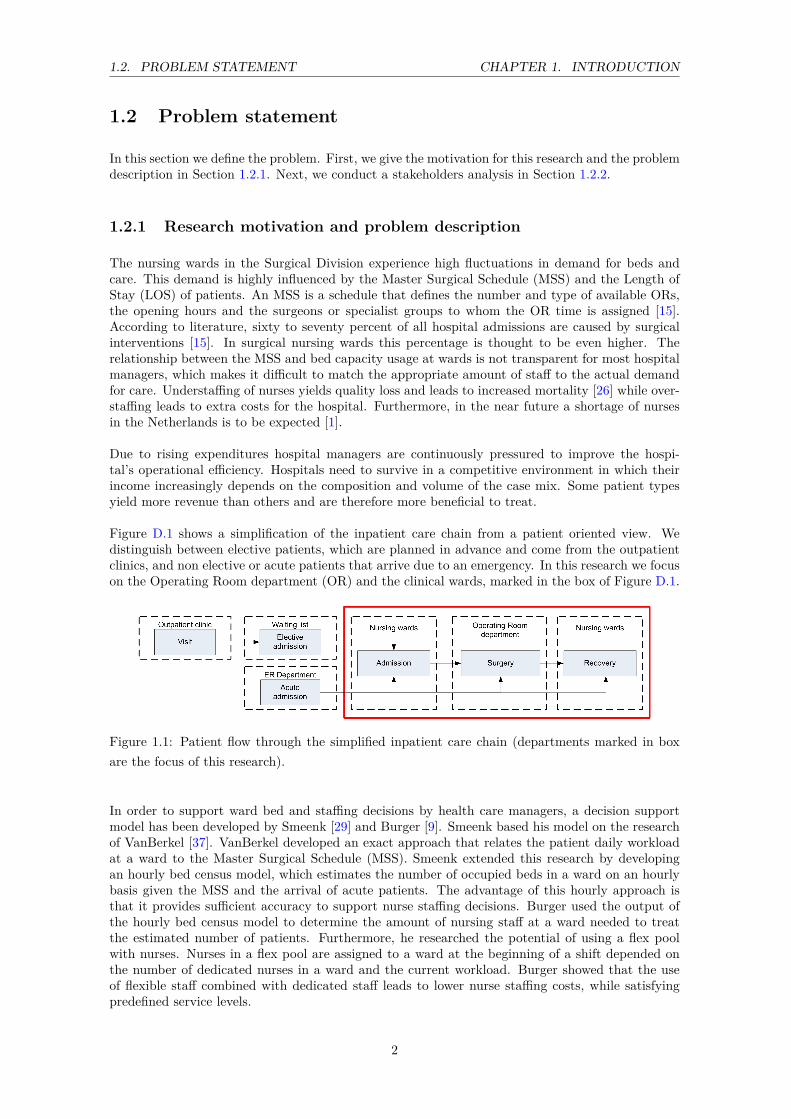
Figure D.1 shows a simplification of the inpatient care chain from a patient oriented view. Wedistinguish between elective patients, which are planned in advance and come from the outpatientclinics, and non elective or acute patients that arrive due to an emergency. In this research we focuson the Operating Room department (OR) and the clinical wards, marked in the box of Figure D.1.

Figure 1.1: Patient flow through the simplified inpatient care chain (departments marked in boxare the focus of this research).

In order to support ward bed and staffing decisions by health care managers, a decision supportmodel has been developed by Smeenk [29] and Burger [9]. Smeenk based his model on the researchof VanBerkel [37]. VanBerkel developed an exact approach that relates the patient daily workloadat a ward to the Master Surgical Schedule (MSS). Smeenk extended this research by developingan hourly bed census model, which estimates the number of occupied beds in a ward on an hourlybasis given the MSS and the arrival of acute patients. The advantage of this hourly approach isthat it provides sufficient accuracy to support nurse staffing decisions. Burger used the output ofthe hourly bed census model to determine the amount of nursing staff at a ward needed to treatthe estimated number of patients. Furthermore, he researched the potential of using a flex poolwith nurses. Nurses in a flex pool are assigned to a ward at the beginning of a shift depended onthe number of dedicated nurses in a ward and the current workload. Burger showed that the useof flexible staff combined with dedicated staff leads to lower nurse staffing costs, while satisfyingpredefined service levels.

2

1.2. PROBLEM STATEMENT CHAPTER 1. INTRODUCTION

The models developed by Smeenk [29] and Burger [9] provide health care managers with a toolto evaluate resource capacity planning decisions on the clinical wards."Resource capacity planningaddresses the dimensioning, planning, scheduling, monitoring, and control of renewable resources"as stated in Hans et al. [16]. By limiting the scope of a project to a single department suboptimalconclusions may be drawn, particularly when the influences of other departments are ignored [37].The next step is to extend the research of Smeenk and Burger by developing a tool that supportshealth care managers in their resource capacity decisions that have an effect on the OR departmentand the clinical wards.

1.2.2 Stakeholder Analysis

We conduct a stakeholder analysis in order to identify the objectives of the various actors in thecare chain (Figure D.1). We discuss the main involved stakeholders (see also Figure 1.2):

Figure 1.2: Overview of the various stakeholders in the inpatient care chain of the AMC.

Board of the hospital: The board is responsible for the long term strategic goals of the hospital.The strategic horizon encompasses decisions concerning one to five years ahead. The overall objec-tive of the board is to achieve high quality care, efficient use of resources, satisfied employees anda financially healthy organisation.

Marketing and control: Marketing and control determines the production volumes for eachspecialty group in cooperation with the different specialties. In addition they negotiate with healthcare insurers on the volume, quality and price of care.

Insurers: Insurers represents the interest of their policy holders. They negotiate with hospi-tals on the quality, volume and price of care.

Patients: Patients demand high quality care at an affordable price. Furthermore, patients arewilling to travel further to receive the best possible care. Access time (time from referral until theday of appointment) and waiting time (on the day of appointment) are increasingly important whenpatients select a hospital.

Specialists: The specialist in the outpatient clinic is responsible for the first contact with a patientand performs the surgery. Specialists deliver good quality of care and demand stable working hours.Because the AMC is an academic hospital the specialists are contracted in-house, compared to nonacademic hospitals where specialist are hired from medical partnerships.

OR management: The OR management is responsible for the strategic decisions that affectthe OR. On a tactical level they allocate capacity to the various specialties. Besides this, they are

3

1.3. RESEARCH OBJECTIVE CHAPTER 1. INTRODUCTION

responsible for coordinating the daily operations inside the OR Department.

OR planner: The OR planner is part of the OR department and responsible for the allocationof ORs, supporting staff and equipment to the specialties. Each specialty has various preferencesand demands. The OR planner strives to meet these preferences and allocate capacity in a fair andtransparent way.

OR personnel: OR personnel consists of an anaesthetist, assistant anaesthetists and surgeryassistants. The OR personnel assists the specialist during surgery. They want to have regularworking hours, smooth transitions between surgeries and a balanced workload.

Division management: A division manages a cluster of specialties in the hospital. The divi-sion management consists of a board and supporting staff. The board is responsible for the longterm vision of a division. The supporting staff performs administrative tasks and monitors thefinancial status for each specialty.

Ward management: The management of a ward is responsible for the daily operations on award. They decide how to allocate the staff to the various shifts and how many operational bedsare available. The ward management wants to provide good quality care, use their resources asefficiently as possible and keep their staff satisfied.

Specialty planner: The specialty planners of the nursing wards schedules patients into fixedsurgery blocks, and aims to maximise patient throughput and to minimise the number of cancelledsurgeries.

Nurses: Nurses have direct contact with patients and largely influence the satisfaction of the pa-tients. Nurses want to have steady working hours and a levelled workload. High variations indemand for care make it difficult for nurses to perform their tasks adequately.

The stakeholder analysis yields various objectives regarding the inpatient care chain:

• Maximise quality of care: Each stakeholder in the inpatient care chain demands a highquality of care. Budget restrictions and variable workloads restrict the solution space of thisobjective.

• Staying financially healthy: The hospital management needs to make sure that the hospitalstays financially healthy.

• Minimise access time: Patients do not want to wait a long time before they can undergosurgery. By using resources more efficiently, access time can be reduced, which is beneficialfor the patients and the hospital’s reputation.

• Minimise underutilisation of resources: The different management layers inside thehospital all want to use their resources efficiently and want to avoid underutilisation.

• Level the workload: A levelled workload leads to satisfied employees that can provide amore constant quality of care.

The above stakeholder analysis makes clear that there are various, conflicting objectives in theinpatient care chain. Due to these conflicting objectives optimisation of the inpatient care chain isvery complex.

1.3 Research objective

We conclude from the previous section that the objective of the hospital management is to createa levelled workload. This will yield a higher quality of care against lower costs. Section 1.2 shows

4

1.3. RESEARCH OBJECTIVE CHAPTER 1. INTRODUCTION

that it is interesting to extend the research of Smeenk [29] and Burger [9] to a model that optimisesresource capacity planning decisions in the OR department and the clinical wards. Furthermore, acost based approach is important for selecting the right mix of patient types. Combining this allleads to the following research objective:

To develop a method which determines the best combination of patient case mix, OR capacity, careunit and nurse staffing decisions in such way that total cost margins are maximised while satisfyingproduction agreements and resource, capacity, and quality constraints.

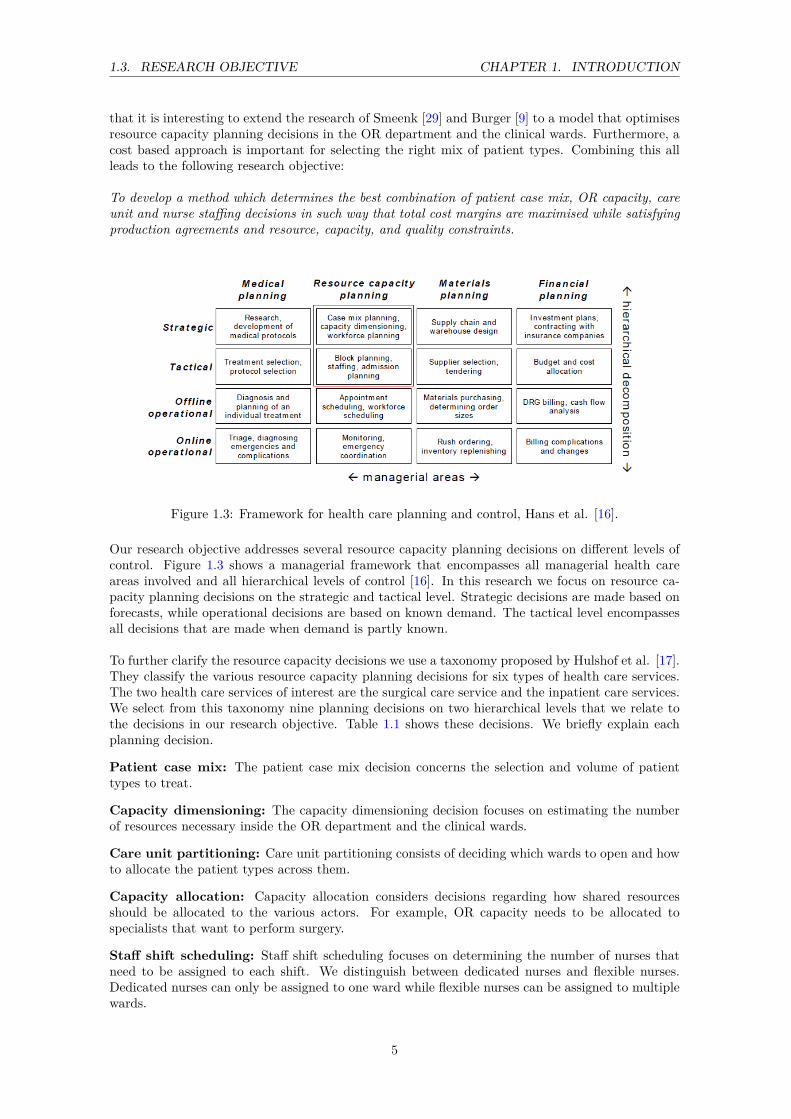
Figure 1.3: Framework for health care planning and control, Hans et al. [16].

Our research objective addresses several resource capacity planning decisions on different levels ofcontrol. Figure 1.3 shows a managerial framework that encompasses all managerial health careareas involved and all hierarchical levels of control [16]. In this research we focus on resource ca-pacity planning decisions on the strategic and tactical level. Strategic decisions are made based onforecasts, while operational decisions are based on known demand. The tactical level encompassesall decisions that are made when demand is partly known.

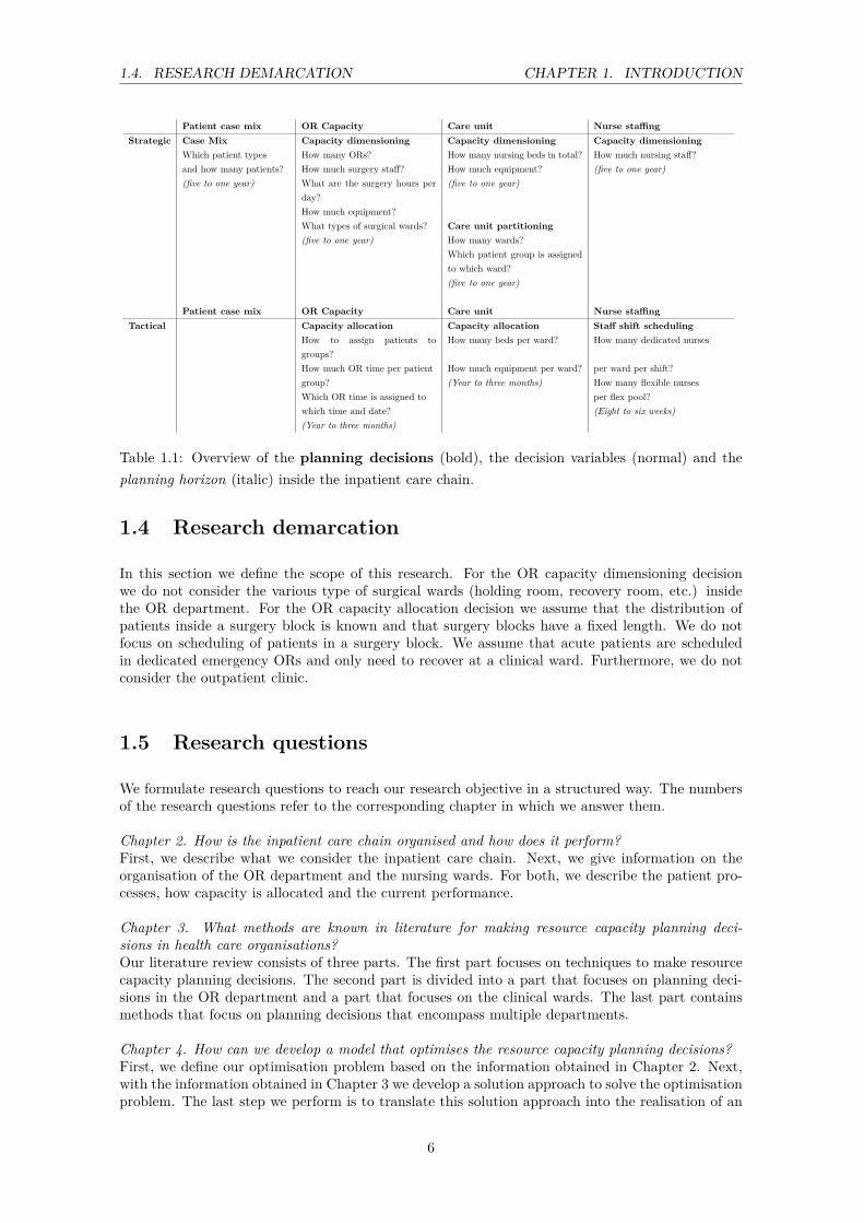
To further clarify the resource capacity decisions we use a taxonomy proposed by Hulshof et al. [17].They classify the various resource capacity planning decisions for six types of health care services.The two health care services of interest are the surgical care service and the inpatient care services.We select from this taxonomy nine planning decisions on two hierarchical levels that we relate tothe decisions in our research objective. Table 1.1 shows these decisions. We briefly explain eachplanning decision.

Patient case mix: The patient case mix decision concerns the selection and volume of patienttypes to treat.

Capacity dimensioning: The capacity dimensioning decision focuses on estimating the numberof resources necessary inside the OR department and the clinical wards.

Care unit partitioning: Care unit partitioning consists of deciding which wards to open and howto allocate the patient types across them.

Capacity allocation: Capacity allocation considers decisions regarding how shared resourcesshould be allocated to the various actors. For example, OR capacity needs to be allocated tospecialists that want to perform surgery.

Staff shift scheduling: Staff shift scheduling focuses on determining the number of nurses thatneed to be assigned to each shift. We distinguish between dedicated nurses and flexible nurses.Dedicated nurses can only be assigned to one ward while flexible nurses can be assigned to multiplewards.

5

1.4. RESEARCH DEMARCATION CHAPTER 1. INTRODUCTION

Patient case mix OR Capacity Care unit Nurse staffingStrategic Case Mix Capacity dimensioning Capacity dimensioning Capacity dimensioning

Which patient types How many ORs? How many nursing beds in total? How much nursing staff?and how many patients? How much surgery staff? How much equipment? (five to one year)(five to one year) What are the surgery hours per

day?(five to one year)

How much equipment?What types of surgical wards? Care unit partitioning(five to one year) How many wards?

Which patient group is assignedto which ward?(five to one year)

Patient case mix OR Capacity Care unit Nurse staffingTactical Capacity allocation Capacity allocation Staff shift scheduling

How to assign patients togroups?

How many beds per ward? How many dedicated nurses

How much OR time per patient How much equipment per ward? per ward per shift?group? (Year to three months) How many flexible nursesWhich OR time is assigned to per flex pool?which time and date? (Eight to six weeks)(Year to three months)

Table 1.1: Overview of the planning decisions (bold), the decision variables (normal) and theplanning horizon (italic) inside the inpatient care chain.

1.4 Research demarcation

In this section we define the scope of this research. For the OR capacity dimensioning decisionwe do not consider the various type of surgical wards (holding room, recovery room, etc.) insidethe OR department. For the OR capacity allocation decision we assume that the distribution ofpatients inside a surgery block is known and that surgery blocks have a fixed length. We do notfocus on scheduling of patients in a surgery block. We assume that acute patients are scheduledin dedicated emergency ORs and only need to recover at a clinical ward. Furthermore, we do notconsider the outpatient clinic.

1.5 Research questions

We formulate research questions to reach our research objective in a structured way. The numbersof the research questions refer to the corresponding chapter in which we answer them.

Chapter 2. How is the inpatient care chain organised and how does it perform?First, we describe what we consider the inpatient care chain. Next, we give information on theorganisation of the OR department and the nursing wards. For both, we describe the patient pro-cesses, how capacity is allocated and the current performance.

Chapter 3. What methods are known in literature for making resource capacity planning deci-sions in health care organisations?Our literature review consists of three parts. The first part focuses on techniques to make resourcecapacity planning decisions. The second part is divided into a part that focuses on planning deci-sions in the OR department and a part that focuses on the clinical wards. The last part containsmethods that focus on planning decisions that encompass multiple departments.

Chapter 4. How can we develop a model that optimises the resource capacity planning decisions?First, we define our optimisation problem based on the information obtained in Chapter 2. Next,with the information obtained in Chapter 3 we develop a solution approach to solve the optimisationproblem. The last step we perform is to translate this solution approach into the realisation of an

6

1.5. RESEARCH QUESTIONS CHAPTER 1. INTRODUCTION

actual model.

Chapter 5. How can we apply our modelling approach to the AMC?In this chapter we perform experiments on data obtained from the Division B of the AMC. First,we apply the model on the current situation. Next, we demonstrate the performance of our solutionapproach by various experiments.

Chapter 6. What are the managerial implications?We conclude this thesis by describing the managerial implications. We summarise our results intoconclusions and give recommendations. Because our research has limitations due to the complex-ity of the various planning decisions we reflect on our approach and provide directions for furtherresearch.

7

Chapter 2

Context analysis

In this research we focus on the clinical wards within the surgical division (Division B) of the AMC.First, Section 2.1 provides key figures of this division. Because hospitals are highly complex systemsand are poorly understood most of the time, these systems are best described by the flow of theirpatients [36]. Section 2.2 describes the patient flow of a patient through the inpatient care chain.Section 2.3 continues with process, control and performance information of the OR department.Section 2.4 contains process, control and performance information of the nursing wards in DivisionB. We end this chapter with conclusions in Section 2.5.

2.1 Division B: surgical specialties

The case study we conduct focuses on Division B, surgical specialties, of the AMC. Table 2.1displays key figures of this division for the year 2010. Currently, this division is in the process ofreorganisation in which the number of wards is reduced to five from seven.

Number of specialties 9Total number of patients per year 8501Total number of wards 7Average LOS in days 5.1Total number of nurses in FTE 161Total number of beds 176

Table 2.1: General characteristics of Division B: surgical specialties for the year 2010 (Source:Braaksma and Kortbeek [8]).

2.2 Patient flow

During the research of Smeenk and Burger [30] an extensive process description of the patient flow,OR department and two nursing wards within this division has been made. The other wards withinthis division have similar processes. We summarise parts of this description and provide additionalinformation. Figure 2.1 shows the different departments that are involved during the stay of thepatient. We make the distinction between elective patients (who are planned) and non elective or

9

2.3. OR DEPARTMENT CHAPTER 2. CONTEXT ANALYSIS

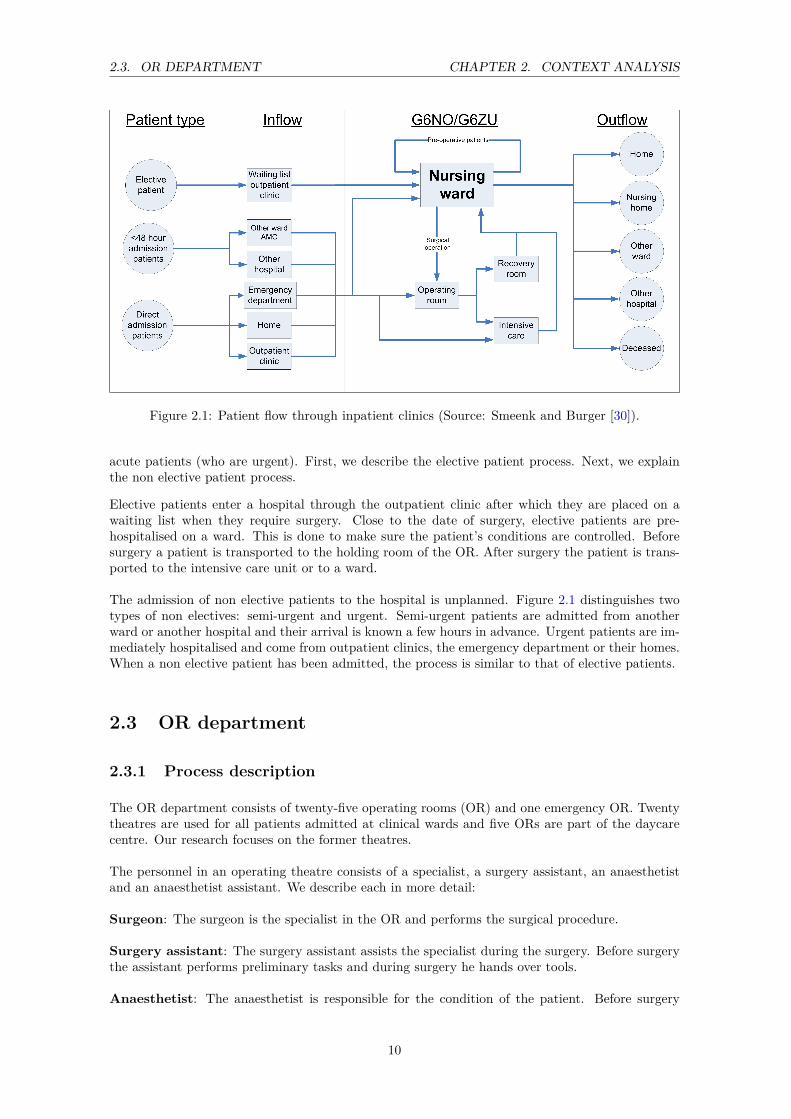
Figure 2.1: Patient flow through inpatient clinics (Source: Smeenk and Burger [30]).

acute patients (who are urgent). First, we describe the elective patient process. Next, we explainthe non elective patient process.

Elective patients enter a hospital through the outpatient clinic after which they are placed on awaiting list when they require surgery. Close to the date of surgery, elective patients are pre-hospitalised on a ward. This is done to make sure the patient’s conditions are controlled. Beforesurgery a patient is transported to the holding room of the OR. After surgery the patient is trans-ported to the intensive care unit or to a ward.

The admission of non elective patients to the hospital is unplanned. Figure 2.1 distinguishes twotypes of non electives: semi-urgent and urgent. Semi-urgent patients are admitted from anotherward or another hospital and their arrival is known a few hours in advance. Urgent patients are im-mediately hospitalised and come from outpatient clinics, the emergency department or their homes.When a non elective patient has been admitted, the process is similar to that of elective patients.

2.3 OR department

2.3.1 Process description

The OR department consists of twenty-five operating rooms (OR) and one emergency OR. Twentytheatres are used for all patients admitted at clinical wards and five ORs are part of the daycarecentre. Our research focuses on the former theatres.

The personnel in an operating theatre consists of a specialist, a surgery assistant, an anaesthetistand an anaesthetist assistant. We describe each in more detail:

Surgeon: The surgeon is the specialist in the OR and performs the surgical procedure.

Surgery assistant: The surgery assistant assists the specialist during the surgery. Before surgerythe assistant performs preliminary tasks and during surgery he hands over tools.

Anaesthetist: The anaesthetist is responsible for the condition of the patient. Before surgery

10

2.3. OR DEPARTMENT CHAPTER 2. CONTEXT ANALYSIS

Figure 2.2: Description of the OR process from a patient oriented view (Source: OK-handleiding[14]).

the anaesthetist checks the condition of the patient and decides if the patient is ready for surgery.During the surgery the anaesthetist continuously monitors the patient’s health and has the powerto abort the surgical procedure.

Anaesthetist assistant: The assistant of the anaesthetist supports the anaesthetist and haslimited decision power.

Figure 2.2 displays the different steps in the OR process. First, a call is made from the OR centreto the designated ward that a patient can be transported to the holding room. A nurse from theward brings the patient to the holding room where the patients wait until the operating theatreis available. When the operating theater is ready, the patient is transported into this theater andthe time-out procedure is started. The time-out procedure consists of verification of the patient,the surgical procedure, the location of the surgical procedure on the patient and it is checked ifall surgical tools needed during surgery are present. Once the time-out procedure is completed theanaesthetist anaesthetises the patient and released him for surgery. When the specialist is finishedthe patient is transported back to the IC or the recovery room of the OR department.

2.3.2 Resource capacity planning and control

In this section we discuss the strategic patient case mix decision and the planning stages concerningthe dimensioning and allocation of OR capacity.

2.3.2.1 Patient case mix

The patient case mix decision concerns the selection and volumes of patient types to treat. Thisdecision ideally depends on the revenue of a patient type, the waiting lists, the facilities and thecontract agreements made with insurers. In the current situation this decision is largely basedon choices made in the pasts. The contract agreements normally take place a few months beforethe start of a new calendar year. In the AMC the department of Marketing and Control (MC)negotiates with insures on behalf of the specialties.

2.3.2.2 OR capacity decisions

We define OR capacity by the following resources: total number of ORs, total amount of staff,opening hours and specialised equipment like x-ray machines. Capacity dimensioning consists ofdeciding how much OR capacity is needed to treat all patients. Capacity allocation consists ofdividing the available capacity over the various specialties. Table 2.2 describes the stages in whichOR capacity is allocated to the specialties in the AMC.

Capacity allocation On a tactical level the OR centre receives a request for OR capacity fromeach division for the upcoming year. This request is based on the annual budget that a division hasavailable to spend on OR capacity. The board of the OR centre balances all requests and assignseach division a total number of surgery hours. These surgery hours are translated to a fixed numberof Operating Room Days (ORDs) per year per specialty. In this phase the total annual OR capacityis assigned to the specialties.

11

2.3. OR DEPARTMENT CHAPTER 2. CONTEXT ANALYSIS

Actor Action Time Period Planning phaseOR Centre Total yearly OR days per

specialtyThree months before anew year

Tactical

OR Centre OR days assigned to spe-cialties

Three months before sur-gical session

Tactical

Specialty planner OR days assigned to sub-specialties

Six weeks before surgicalsession

Tactical

Surgeon Patient planned intoblocks of subspecialties

Thursday week before sur-gical session

Offline operational

OR Centre Creation of definite surgi-cal schedule

Thursday week before sur-gical session

Offline operational

OR Centre Daily scheduling of surg-eries

On day of the surgical ses-sion

Online operational

Table 2.2: Overview of the AMC planning stages of OR capacity (Source: Smeenk and Burger,OK-handleiding [30, 14]).

Next, the ORDs assigned to each specialty are transformed by the OR centre into a Master SurgicalSchedule (MSS) that states the number of surgery blocks a specialty can use for each day of a year.This MSS has a rolling horizon of twelve months and does not change in the last three monthsbefore execution. The speciality planner of a division receives the final schedule three months be-fore execution and subdivides the ORDs into full, morning and afternoon ORDs. Each specialtyplanner of the division uses her own method to plan surgery blocks. For example, the specialtyplanner of General Surgery uses a basic assignment method [29] to divide the available ORDs to thesubspecialties. Other specialty planners assign blocks to surgeons and some directly plan patientson a first come first serve basis. During interviews with the specialty planners we received variousremarks about the high variation in number of ORDs that a specialty receives from the OR centreeach month. This high variation makes it difficult to predict the number of ORDs available and tocreate a standardised planning method.

Operational planning The operational level consists of an offline and online operational planning.On an offline operational level the patients are planned into sub specialty blocks by the specialistthat performs the surgery. Once the surgeries are planned, the OR schedule is updated and finishedby the OR centre. The last surgery in the operational schedule can be marked Pro Memorie (PM)when there is high variance in scheduled surgery times or when there is a schedule that is too tight.A surgery marked PM has a high probability to be cancelled when other surgeries are delayed.The OR centre is responsible for the online operational planning in which non elective patients arescheduled.

Non elective patients at the OR department are classified by four categories: acute, urgent, semi-urgent and semi-elective. The first two categories preferably undergo surgery in the emergency OR.When the emergency OR is occupied the OR centre can decide to break into an elective sched-ule. The semi-urgent and semi-elective surgeries are preferably performed in ORs assigned to thatspecific specialty.

2.3.3 Performance

In this section we evaluate the performance of the OR department. We use available informationfrom the management information system Cognos. Because a detailed in-depth research in the ORdepartment is not possible within the available time frame we focus on describing the performanceindicators present of this information system. First, we introduce five definitions which are needed

12

2.3. OR DEPARTMENT CHAPTER 2. CONTEXT ANALYSIS

to understand the performance indicators. Next, we describe the performance indicators and showthe values for the year 2010.

We have the following definitions:

• Budgeted hours: Total surgery hours per year assigned to each specialty by the OR centre.These budgeted hours are allocated but not scheduled yet.

• Realised budgeted hours: Total hours actually scheduled in the Master Surgical Scheduleby the OR centre. This value may differ from the budgeted hours.

• Planned hours: The total amount of hours per year that a specialty planner or specialistactually plans with elective patients.

• Realised hours: The total amount of hours per year that a specialty uses the OR duringnormal working hours. This value does not include overtime, but does includes the treatmentof acute patients during regular surgery hours.

• Overtime hours: The total amount of surgery hours per year that a specialty used inovertime.

We give a numerical example of how the definitions can be interpreted. For example, a specialtyrequests 110 surgery hours but receives 100 budgeted hours from the OR centre. From this 100budgeted hours, 90 hours are actually assigned by the OR centre to ORDs. The other 10 hours arenot assigned due for example a shortage of nursing assistants. A specialty plans 70 hours of the 90realised budgeted hours, while it in reality uses 80 hours to perform all planned and non electivesurgeries. Off these 80 hours 5 hours are used during overtime.

We consider the following performance indicators:

Budget realisation: This is the percentage of budgeted hours that is actually scheduled by theOR centre to the various specialties. We determine this indicator by dividing the realised budgethours by the budgeted hours.

Planning utilisation: This performance indicator states the percentage of hours actual plannedcompared to the budget realisation. We calculate this indicator by dividing the planned hours bythe realised budgeted hours.

Realised utilisation: This performance indicator states how efficient the OR is used duringassigned hours. We calculate this indicator by dividing the realised hours by realised budget hours.

Overtime utilisation: This performance indicator states how much of the OR time assignedis spend on overtime. We determine this indicator by dividing the overtime hours by realised bud-get hours added with the over time hours.

Cancellation rate: Total number of surgeries cancelled by the hospital divided by the totalnumber of scheduled surgeries.

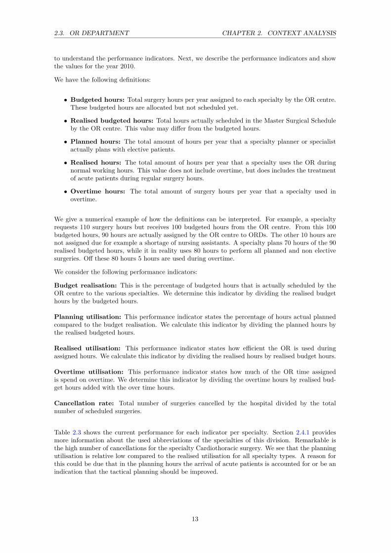
Table 2.3 shows the current performance for each indicator per specialty. Section 2.4.1 providesmore information about the used abbreviations of the specialties of this division. Remarkable isthe high number of cancellations for the specialty Cardiothoracic surgery. We see that the planningutilisation is relative low compared to the realised utilisation for all specialty types. A reason forthis could be due that in the planning hours the arrival of acute patients is accounted for or be anindication that the tactical planning should be improved.

13

2.4. INPATIENT CARE UNITS CHAPTER 2. CONTEXT ANALYSIS

Indicator CAP CHI CHP MZK ORT UROBudgeted hours 5766 6847 1426 566 1836 1588Budget realisation 91.4% 89.6% 92.2% 92.2% 75.5% 92.0%Planned utilisation 72.7% 80.3% 79.3% 79.5% 77.8% 69.1%Realised utilisation 83.0% 87.0% 83.7% 82.5% 86.9% 86.2%Overtime utilisation 10.8% 4.4% 3.7% 3.6% 4.7% 3.6%Cancellation rate 12.8% 5.0% 5.7% 3.9% 7.8% 6.9%

Table 2.3: Overview of the performance of the OR department for each specialty for the year 2010(Source: Cognos 2011).

2.4 Inpatient care units

In this section we discuss the nursing wards within division B. Section 2.4.1 discusses the actorsinvolved and the patient process. Section 2.4.2 describes how the capacity of a nursing ward isallocated and the assignment of nurses to shifts. Section 2.4.3 states the current performance ofthe nursing wards in terms of misplacements and the realised bed census.

2.4.1 Process

The surgical specialties division consists of seven wards to which nine different patient types areassigned. Table 2.4 provides an overview of these types and their designated wards for the year2010.

Cluster Specialty Patientgroup WardCAP CAP Cardiothorcal surgery G3ZCHI CHI General surgery G6NCHI CHI General surgery G6ZCHI CHIss Short stay surgery G5NCHP CHP Plastic surgery G5ZMZK MZK Oral pathology and maxilla surgery G6ZMZK ORT Orthopedic surgery G7ZTRA TRA Traumatology G7NURO URO Urology G5NCHI VAA Vascular surgery G5Z

Table 2.4: General characteristics of patient groups of the Division B: surgical specialties for theyear 2010 (Source: Braaksma and Kortbeek [8]).

A ward can be characterised by the number of beds, the patient types and the total amount ofavailable personnel. The wards all have twenty four operational beds except for ward G5 Noord,which has thirty operational beds [8]. Each patient group requires a different type of medical careand has an unique length of stay (LOS). The staff at a ward can be categorised into nursing, med-ical, and administrative staff, of which nursing is the largest group. The working hours at a wardare divided into three shifts: day, evening, and night. For a more extensive description of staff,working hours and tasks we refer to the process description by Smeenk and Burger [30].

From a patient-oriented view we can distinguish three steps, admission, stay, and discharge. Apatient is admitted at a ward either because he is scheduled for surgery, another procedure, or he

14

2.4. INPATIENT CARE UNITS CHAPTER 2. CONTEXT ANALYSIS

needs urgent medical care. The LOS of a patient is the time between admission and discharge.During the stay of a patient he undergoes surgery and recovers. When the doctor declares thepatient healthy he is discharged from the ward and can go home.

2.4.2 Resource capacity planning and control

We define the capacity of a ward by the following three resources: the number of available beds,specialised equipment and assigned staff. How this capacity is utilised depends on the allocationof beds and the scheduling of nurses. Section 2.4.2.1 discusses control decisions related to the careunits. Section 2.4.2.2 states the decisions related to nurse scheduling.

2.4.2.1 Care unit decisions

In this section, we discuss the resource capacity planning decisions in the care units. First, weprovide information on the allocation of patients to care units. Next, we briefly describe how thecapacity is determined. We end this section by describing the operational admission planning andcontrol.

Care unit partitioning Care unit partitioning consists of two interrelated decisions. How manywards do we need to open and how should we assign the different patient types to them? Thisdecision is made by the division management. Traditionally, each specialty is allocated to an ownward [31]. In the AMC, specialties with a low number of patients per type are combined andspecialties with a high number of patients per type have their own individual ward.

Capacity dimensioning Capacity dimensioning of a ward consists of determination of the numberof operational beds and equipment necessary to treat all patients. This decision is made by divisionmanagement in cooperation with ward management.

Admission control Admission control of patients consists of two operational planning phases.Wards are informed about elective surgeries one or two weeks in advance that are scheduled forsurgery. The head nurse then decides if a patient can be admitted to their ward and at what time.If the ward is expected to be occupied by other admissions the patient is assigned to an otherward. On the admission day of the patient the head nurse evaluates the current bed occupationand the other planned admissions. When there is no room to admit the patient the head nurse canreallocate a planned admission to another ward. Acceptance of non elective patients depends onthe current bed occupation and the planned admissions for the upcoming days.

2.4.2.2 Nurse scheduling decisions

In this section we discuss decisions related to the scheduling of nurses. First, we state the capacitydimensioning decision. Next we describe how the number of nurses per shift are determined in thecurrent situation.

Capacity dimensioning Capacity dimensioning consists of determining the total amount of staffneeded. Because contractual agreements with employees are made for a long term this must bedone accurately. The contract negotiations are done by the management of each ward.

Staff shift scheduling Staff shift scheduling consists of determining the number of nurses neededper shift. Ward management is responsible for this decision. The offline operational nursing rosteris created ten weeks in advance by the planner of the ward, when the demand resulting from themaster surgical schedule is still unknown. In at least two wards, the management chooses to assignthe same total number of nurses to a shift for each day of the week. This total number is basedon the maximum number of operational beds and the patient-to-nurse ratio during each shift. Thepatient-to-nurse ratio describes how many patients a nurse can care for and depends on the shift.

15

2.4. INPATIENT CARE UNITS CHAPTER 2. CONTEXT ANALYSIS

On an online operational level nurses can become ill and the number of operational beds at a wardis reduced. Another option is to hire additional workers to replace these ill nurses.

2.4.3 Performance

We describe the performance of a nursing ward by the misplacement rate and the rejection rate,and the realised bed census. We discuss the misplacement rejection rates first. Next, we evaluatethe realised bed census.

A misplacement occurs when a patient is placed in a non dedicated ward. A rejection occurs when apatient is refused by the hospital. Table 2.4 shows the dedicated or preferred ward for each patienttype of Division B for the year 2010. We determine the misplacement rates from 2010 as follows.We count the number of admissions of each patient type in their non dedicated ward and dividethis by the total number of admission for this specific patient type. We clustered the surgical shortstay and general surgery patient types because these could not be separated in the data. Table2.5 shows the misplacement rates for each specialty. The specialty CAP has a misplacement rateof zero because these patients need specific equipment, which is only available in their designatedward. We can not measure the rejection rate because no information is available about the numberof rejections per patient type.

Specialty Nr admissions designated ward Total admission Misplacement ratioCAP 1816 1816 0.0%CHI 2732 2789 2.0%CHP 470 491 4.3%MZK 189 205 7.8%ORT 1179 1228 4.0%TRA 1041 1064 2.2%URO 1139 1147 0.7%VAA 543 554 2.0%

Table 2.5: Admission and misplacements for each specialty for the year 2010 (Source: Locati 2011).

The bed census states the number of operational beds used during a day of the week. Figure 2.3shows a box plot of the bed occupancy for each day of the week for the wards under discussion. Thegreen dotted line gives the maximum number of beds on each of the wards. The upper percentileof the bed census for some wards in the box plot can go above this line because wards have thepossibility to add additional beds in case of extreme demand. Figure 2.3 shows that the averagenumber of occupied beds lies far below the maximum number of operational beds that is used tostaff nurses. When we look at the distribution of demand we denote that the values hive a highvariation on each day of the week. The average bed census of ward G7NO is particularly lowcompared to the maximum and this ward is favourite to misplace patients to.

16

2.4. INPATIENT CARE UNITS CHAPTER 2. CONTEXT ANALYSIS

(a) G3ZU (b) G5NO

(c) G5ZU (d) G6NO

(e) G6ZU (f) G7NO

(g) G7ZU

Figure 2.3: Average bed census for each day of the week for wards of Division B, in which thegreen dotted line states the maximum number of beds, 8500 admissions, year 2010 (Source: Cognos2011).

17

2.5. CONCLUSIONS CHAPTER 2. CONTEXT ANALYSIS

2.5 Conclusions

In this chapter we analysed the OR department and the clinical wards of Division B. We identifiedthe following causes that may yield inefficient resource usage:

• A fluctuating block scheduleThe current Operating Room Days (ORDs) assigned to the specialties differs monthly. Vari-ation in the number of surgery blocks scheduled results in variation of demand for care at theinpatient care units.

• No standardisation in scheduling of patients for surgeryEach specialty planner has its individual method of scheduling patients into surgery blocks.Due to lack of standardisation between the specialties it is difficult to predict the impact of ascheduled surgery block on the bed occupation in a ward.

• Nurses are scheduled based on static demandThe scheduling of nurses is based on the maximum number of beds per ward and the patient-to-nurse ratio per shift for each day of the week. The actual demand is dynamic and differseach day and each hour. In at least two of the wards, the required number of nurses is basedon the maximum demand, which results in overstaffing.

• Mismatch of planning horizonsIn order to schedule nurses based on a dynamic demand we need two consecutive steps. First,we need to know the demand resulting from the MSS and the arrival of acute patients. Next,we need to align both planning horizons. Currently, the scheduling of nurses is performedten weeks in advance. At this moment in time, the demand caused by the MSS is partlyunknown, because the scheduling of patients in a surgery block is performed two to threeweeks in advance. This mismatch in planning horizons makes it difficult to adequately staffthe right number of nurses to a shift.

• Relatively small ward sizesThe ward sizes under consideration are relatively small. Due to these small ward sizes thedemand for care is highly influenced by how the surgery blocks, and the patient inside asurgery block, are scheduled.

All of the causes above indicate that the processes in the inpatient care chain can be improved andthat resources can be used more efficiently. To reduce variation in the demand for beds, severalpatient types could be combined into the same ward to obtain benefits of the risk pool effect. Otheropportunities lie in the integral development of a cyclic MSS that minimises the total resourcesneeded at the clinical nursing wards and better aligns the planning horizon of the scheduling ofnurses with the MSS.

18

Chapter 3

Literature

This chapter describes literature related to resource capacity planning in health care. For a taxo-nomic classification of planning decisions in health care and a state of the art review we refer toHulshof et al. [17].

We structured this chapter as follows. First, we provide an overview of the techniques in literaturefor making resource capacity planning decisions in Section 3.1. Next, we discuss resource capacityplanning methods for the OR department in Section 3.2. Section 3.3 states the planning methods fornursing wards. Section 3.4 describes various decomposition approaches for optimisation of multipleplanning decisions. Section 3.5 states the conclusions of this chapter.

3.1 Techniques for resource capacity planning

Within the Operational Research/ Management Science literature several models are presentedto support resource capacity planning decisions. These models can be broadly characterised asanalytical or simulation based [35]. Most of the time analytical optimisation methods require onlyone experimental run to produce optimal or near optimal solutions [18] while simulation optimisationfocuses on finding the best input variables from all possible combinations without evaluating eachpossibility [12]. The strength of simulation models lies in the fact that they are well equipped tocapture the broad scope of complex systems [36] while analytical methods have a limited capacityto characterise these systems. A possible weakness of simulation based optimisation is that thesemodels are inexact and require a great deal of time to develop [36]. For a literate review of articlesin which analytical and simulation techniques are used in the operating theatres we refer to Cardoenet al. [11]. For a more elaborated overview of simulation techniques in hospital settings we refer toJun et al. [18].

To overcome the disadvantages of both simulation and analytical models several researchers havedeveloped methods that combine the strength of both techniques. We provide one example: Cochranet al. [13] propose a method for stochastic bed balancing inside an obstetrics hospital. First,an analytical queueing model is developed to asses the flow between units. Next, discrete-eventsimulation is used to maximise the flow through the balanced system and to study several what-ifscenarios.

19

3.2. METHODS OR DEPARTMENT CHAPTER 3. LITERATURE

3.2 Resource capacity planning methods for the OR depart-ment

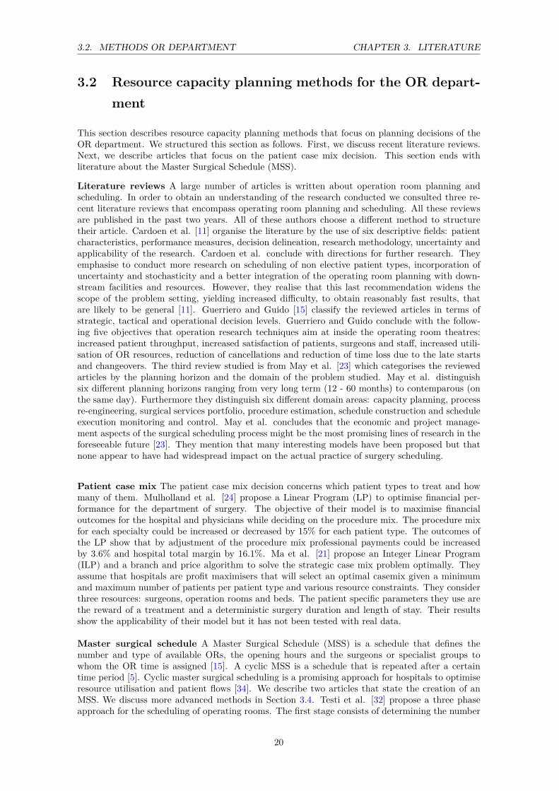
This section describes resource capacity planning methods that focus on planning decisions of theOR department. We structured this section as follows. First, we discuss recent literature reviews.Next, we describe articles that focus on the patient case mix decision. This section ends withliterature about the Master Surgical Schedule (MSS).

Literature reviews A large number of articles is written about operation room planning andscheduling. In order to obtain an understanding of the research conducted we consulted three re-cent literature reviews that encompass operating room planning and scheduling. All these reviewsare published in the past two years. All of these authors choose a different method to structuretheir article. Cardoen et al. [11] organise the literature by the use of six descriptive fields: patientcharacteristics, performance measures, decision delineation, research methodology, uncertainty andapplicability of the research. Cardoen et al. conclude with directions for further research. Theyemphasise to conduct more research on scheduling of non elective patient types, incorporation ofuncertainty and stochasticity and a better integration of the operating room planning with down-stream facilities and resources. However, they realise that this last recommendation widens thescope of the problem setting, yielding increased difficulty, to obtain reasonably fast results, thatare likely to be general [11]. Guerriero and Guido [15] classify the reviewed articles in terms ofstrategic, tactical and operational decision levels. Guerriero and Guido conclude with the follow-ing five objectives that operation research techniques aim at inside the operating room theatres:increased patient throughput, increased satisfaction of patients, surgeons and staff, increased utili-sation of OR resources, reduction of cancellations and reduction of time loss due to the late startsand changeovers. The third review studied is from May et al. [23] which categorises the reviewedarticles by the planning horizon and the domain of the problem studied. May et al. distinguishsix different planning horizons ranging from very long term (12 - 60 months) to contemparous (onthe same day). Furthermore they distinguish six different domain areas: capacity planning, processre-engineering, surgical services portfolio, procedure estimation, schedule construction and scheduleexecution monitoring and control. May et al. concludes that the economic and project manage-ment aspects of the surgical scheduling process might be the most promising lines of research in theforeseeable future [23]. They mention that many interesting models have been proposed but thatnone appear to have had widespread impact on the actual practice of surgery scheduling.

Patient case mix The patient case mix decision concerns which patient types to treat and howmany of them. Mulholland et al. [24] propose a Linear Program (LP) to optimise financial per-formance for the department of surgery. The objective of their model is to maximise financialoutcomes for the hospital and physicians while deciding on the procedure mix. The procedure mixfor each specialty could be increased or decreased by 15% for each patient type. The outcomes ofthe LP show that by adjustment of the procedure mix professional payments could be increasedby 3.6% and hospital total margin by 16.1%. Ma et al. [21] propose an Integer Linear Program(ILP) and a branch and price algorithm to solve the strategic case mix problem optimally. Theyassume that hospitals are profit maximisers that will select an optimal casemix given a minimumand maximum number of patients per patient type and various resource constraints. They considerthree resources: surgeons, operation rooms and beds. The patient specific parameters they use arethe reward of a treatment and a deterministic surgery duration and length of stay. Their resultsshow the applicability of their model but it has not been tested with real data.

Master surgical schedule A Master Surgical Schedule (MSS) is a schedule that defines thenumber and type of available ORs, the opening hours and the surgeons or specialist groups towhom the OR time is assigned [15]. A cyclic MSS is a schedule that is repeated after a certaintime period [5]. Cyclic master surgical scheduling is a promising approach for hospitals to optimiseresource utilisation and patient flows [34]. We describe two articles that state the creation of anMSS. We discuss more advanced methods in Section 3.4. Testi et al. [32] propose a three phaseapproach for the scheduling of operating rooms. The first stage consists of determining the number

20

3.3. METHODS CLINICAL WARDS CHAPTER 3. LITERATURE

of sessions per type to schedule based on the demand and the available operating room time. Inthe second stage an ILP is solved that assigns the session time from the first stage to available ORdays. The objective of this ILP is to maximise surgeon’s preferences. The last stage consists ofa simulation model in which various heuristics are used to assign patient types to surgical blocks.Van Oostrum et al. [33] propose a two phase master surgical scheduling approach at the tacticallevel. First, they create a set of operating room days (ORDs) in which patient types are scheduledby means of column generation with the objective to reach a target utilisation. Next, an ILP isformulated to assign ORDs to actual days of the MSS with the objective to level the bed occupation.

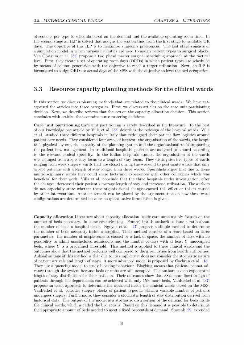
3.3 Resource capacity planning methods for the clinical wards

In this section we discuss planning methods that are related to the clinical wards. We have cat-egorised the articles into three categories. First, we discuss articles on the care unit partitioningdecision. Next, we describe reviews that focuses on the capacity allocation decision. This sectionconcludes with articles that contains nurse rostering decisions.

Care unit partitioning Care unit partitioning is rarely described in the literature. To the bestof our knowledge one article by Villa et al. [38] describes the redesign of the hospital wards. Villaet al. studied three different hospitals in Italy that redesigned their patient flow logistics aroundpatient care needs. They considered four areas of interest: the organisation of the wards, the hospi-tal’s physical lay-out, the capacity of the planning system and the organisational roles supportingthe patient flow management. In traditional hospitals, patients are assigned to a ward accordingto the relevant clinical specialty. In the Italian hospitals studied the organisation of the wardswas changed from a specialty focus to a length of stay focus. They distinguish five types of wardsranging from week surgery wards that are closed during the weekend to post-acute wards that onlyaccept patients with a length of stay longer than three weeks. Specialists argue that due to thesemultidisciplinary wards they could share facts and experiences with other colleagues which wasbeneficial for their work. Villa et al. conclude that the three hospitals under investigation, afterthe changes, decreased their patient’s average length of stay and increased utilisation. The authorsdo not especially state whether these organisational changes caused this effect or this is causedby other interventions. Another remark can be placed by the argumentation on how these wardconfigurations are determined because no quantitative formulation is given.

Capacity allocation Literature about capacity allocation inside care units mainly focuses on thenumber of beds necessary. In some countries (e.g. France) health authorities issue a ratio aboutthe number of beds a hospital needs. Nguyen et al. [27] propose a simple method to determinethe number of beds necessary inside a hospital. Their method consists of a score based on threeparameters: the number of misplacements caused by a lack of space, the number of days with nopossibility to admit unscheduled admissions and the number of days with at least U unoccupiedbeds, where U is a predefined threshold. This method is applied to three clinical wards and theoutcomes show that the method performs well compared to the given ratios from health authorities.A disadvantage of this method is that due to its simplicity it does not consider the stochastic natureof patient arrivals and length of stays. A more advanced model is proposed by Cochran et al. [13].They use a queueing model to study blocking behaviour. Blocking means that patients cannot ad-vance through the system because beds or units are still occupied. The authors use an exponentiallength of stay distribution for their patients. Their outcomes show that 38% more flowthrough ofpatients through the departments can be achieved with only 15% more beds. VanBerkel et al. [37]propose an exact approach to determine the workload inside the clinicial wards based on the MSS.VanBerkel et al. consider surgery blocks of patient types in which a variable number of patientsundergoes surgery. Furthermore, they consider a stochastic length of stay distribution derived fromhistorical data. The output of the model is a stochastic distribution of the demand for beds insidethe clinical wards, which is called the bed census. Based on this demand it is possible to determinethe appropriate amount of beds needed to meet a fixed percentile of demand. Smeenk [29] extended

21

3.4. DECOMPOSITION APPROACHES CHAPTER 3. LITERATURE

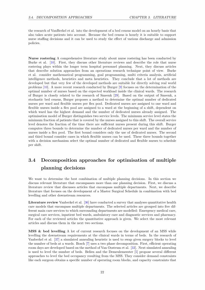
the research of VanBerkel et al. into the development of a bed census model on an hourly basis thatalso takes acute patients into account. Because the bed census is hourly it is suitable to supportnurse staffing decisions and it can be used to study the effect of various discharge and admissionpolicies.

Nurse rostering A comprehensive literature study about nurse rostering has been conducted byBurke et al. [10]. First, they discuss other literature reviews and describe the role that nurserostering plays within the longer term hospital personnel planning. Next, they discuss articlesthat describe solution approaches from an operations research technique point of view. Burkeet al. consider mathematical programming, goal programming, multi criteria analysis, artificialintelligence methods, heuristics and meta heuristics. They conclude that a lot of methods aredeveloped but that very few of the developed methods are suitable for directly solving real worldproblems [10]. A more recent research conducted by Burger [9] focuses on the determination of theoptimal number of nurses based on the expected workload inside the clinical wards. The researchof Burger is closely related to the research of Smeenk [29]. Based on the output of Smeenk, astochastic bed census, Burger proposes a method to determine the optimal number of dedicatednurses per ward and flexible nurses per flex pool. Dedicated nurses are assigned to one ward andflexible nurses inside a flex pool are assigned to a ward at the beginning of a shift, dependent onwhich ward has the highest demand and the number of dedicated nurses already assigned. Theoptimisation model of Burger distinguishes two service levels. The minimum service level states theminimum fraction of patients that is covered by the nurses assigned to this shift. The overall servicelevel denotes the fraction of the time there are sufficient nurses present during this shift. Burgercomputes three bounds to determine the number of dedicated nurses per ward and the number ofnurses inside a flex pool. The first bound considers only the use of dedicated nurses. The secondand third bound consider cases in which flexible nurses can be used. These three bounds togetherwith a decision mechanism select the optimal number of dedicated and flexible nurses to scheduleper shift.

3.4 Decomposition approaches for optimisation of multipleplanning decisions

We want to determine the best combination of multiple planning decisions. In this section wediscuss relevant literature that encompasses more than one planning decision. First, we discuss aliterature review that discusses articles that encompass multiple departments. Next, we describeliterature that focuses on the development of a Master Surgical Schedule in combination with bedlevelling and other downstream resources.

Literature review Vanberkel et al. [36] have conducted a survey that analyses quantitative healthcare models that encompass multiple departments. The selected articles are grouped into five dif-ferent main care services to which surrounding departments are modelled: Emergency medical care,surgical care services, inpatient bed wards, ambulatory care and diagnostic services and pharmacy.For each of the reviewed articles the quantitative approach is given. We select the most relevantarticles and discuss them in the next two sections.

MSS & bed levelling A lot of current research focuses on the development of an MSS whilelevelling the downstream requirements at the clinical wards in terms of beds. In the research ofVanberkel et al. [37] a simulated annealing heuristic is used to swap given surgery blocks to levelthe number of beds at a wards. Bosch [7] uses a two phase decomposition. First, efficient operatingroom days are developed based on the method of Van Oostrum et al. [33]. Next simulated annealingis used to level the number of beds. Belïen and the Demeulemeester [5] propose several differentapproaches to level the bed occupancy resulting from the MSS. They consider demand constraintslike each surgeon obtains a specific number of operating room blocks, and capacity constraints that

22

3.5. CONCLUSIONS CHAPTER 3. LITERATURE

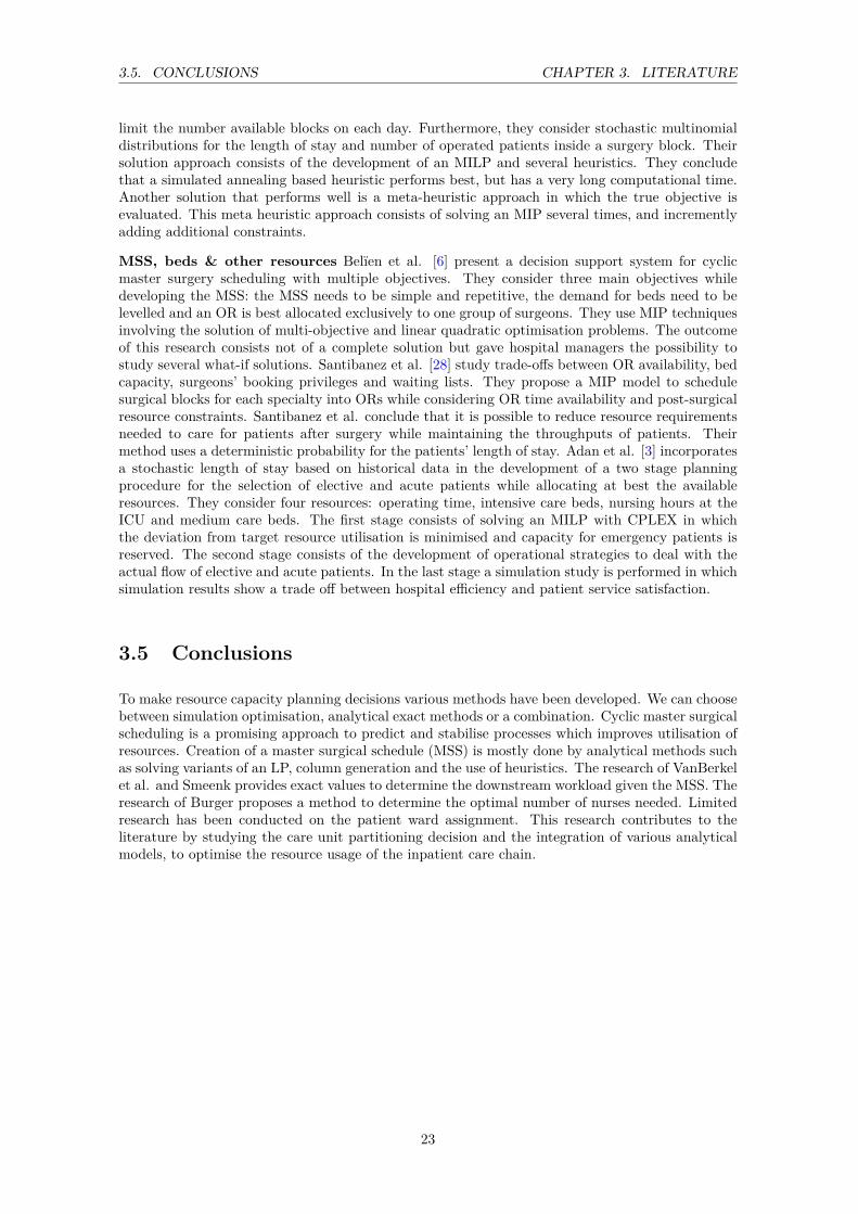
limit the number available blocks on each day. Furthermore, they consider stochastic multinomialdistributions for the length of stay and number of operated patients inside a surgery block. Theirsolution approach consists of the development of an MILP and several heuristics. They concludethat a simulated annealing based heuristic performs best, but has a very long computational time.Another solution that performs well is a meta-heuristic approach in which the true objective isevaluated. This meta heuristic approach consists of solving an MIP several times, and incrementlyadding additional constraints.

MSS, beds & other resources Belïen et al. [6] present a decision support system for cyclicmaster surgery scheduling with multiple objectives. They consider three main objectives whiledeveloping the MSS: the MSS needs to be simple and repetitive, the demand for beds need to belevelled and an OR is best allocated exclusively to one group of surgeons. They use MIP techniquesinvolving the solution of multi-objective and linear quadratic optimisation problems. The outcomeof this research consists not of a complete solution but gave hospital managers the possibility tostudy several what-if solutions. Santibanez et al. [28] study trade-offs between OR availability, bedcapacity, surgeons’ booking privileges and waiting lists. They propose a MIP model to schedulesurgical blocks for each specialty into ORs while considering OR time availability and post-surgicalresource constraints. Santibanez et al. conclude that it is possible to reduce resource requirementsneeded to care for patients after surgery while maintaining the throughputs of patients. Theirmethod uses a deterministic probability for the patients’ length of stay. Adan et al. [3] incorporatesa stochastic length of stay based on historical data in the development of a two stage planningprocedure for the selection of elective and acute patients while allocating at best the availableresources. They consider four resources: operating time, intensive care beds, nursing hours at theICU and medium care beds. The first stage consists of solving an MILP with CPLEX in whichthe deviation from target resource utilisation is minimised and capacity for emergency patients isreserved. The second stage consists of the development of operational strategies to deal with theactual flow of elective and acute patients. In the last stage a simulation study is performed in whichsimulation results show a trade off between hospital efficiency and patient service satisfaction.

3.5 Conclusions

To make resource capacity planning decisions various methods have been developed. We can choosebetween simulation optimisation, analytical exact methods or a combination. Cyclic master surgicalscheduling is a promising approach to predict and stabilise processes which improves utilisation ofresources. Creation of a master surgical schedule (MSS) is mostly done by analytical methods suchas solving variants of an LP, column generation and the use of heuristics. The research of VanBerkelet al. and Smeenk provides exact values to determine the downstream workload given the MSS. Theresearch of Burger proposes a method to determine the optimal number of nurses needed. Limitedresearch has been conducted on the patient ward assignment. This research contributes to theliterature by studying the care unit partitioning decision and the integration of various analyticalmodels, to optimise the resource usage of the inpatient care chain.

23

Chapter 4

Solution approach

In this chapter we describe our solution approach to reach our research objective. Section 4.1formulates the research objective as a mathematical optimisation problem. In this section weelaborate on the relationships between the various planning decisions and constraints we take intoaccount. Section 4.2 describes our decomposition approach to solve this optimisation problem.We describe the technical implementation of our model in Section 4.3. Section 4.4 contains theverification and validation. Section 4.5 concludes with our conclusions.

4.1 Optimisation problem

In the upcoming sections we systematically formulate our research objective as a mathematicaloptimisation problem. Section 4.1.1 contains the assumption we make. Section 4.1.2 describesthe relationship between the resource capacity planning decisions and the constraints we take intoaccount. We formulate the objective function and describe cost parameters in Section 4.1.3. Weconclude this section with an overview of the performance indicators in Section 4.1.4.

4.1.1 Assumptions

To reduce modelling complexity we make the following assumptions:

• Acute patients arrive directly at the ward according to a non-homogeneous Poisson distribu-tion. This means that acute patients in our model do not use the OR and directly arrive ata ward.

• A surgery block only contains patients of the same type. This implies that each patient fromthe same surgery block is assigned to the same ward.

4.1.2 Decisions

Figure 4.1 shows the relationships between the various planning decisions as described in Section1.3. Some decisions are marked green and others are marked orange. In Section 4.1.2.1 to Section4.1.2.3 we explore the mathematical relations between the planning decisions. Based on theserelations we show that when we make the decisions marked in orange we automatically make thedecisions marked in green. Section 4.1.2.1 discusses decisions regarding OR capacity allocation.

25

4.1. OPTIMISATION PROBLEM CHAPTER 4. SOLUTION APPROACH

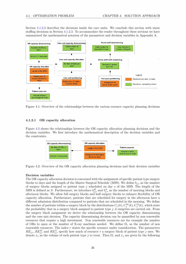
Section 4.1.2.2 describes the decisions inside the care units. We conclude this section with nursestaffing decisions in Section 4.1.2.3. To accommodate the reader throughout these sections we havesummarised the mathematical notation of the parameters and decision variables in Appendix A.

Figure 4.1: Overview of the relationships between the various resource capacity planning decisions

4.1.2.1 OR capacity allocation

Figure 4.2 shows the relationships between the OR capacity allocation planning decisions and thedecision variables. We first introduce the mathematical description of the decision variables andthe constraints.

Figure 4.2: Overview of the OR capacity allocation planning decisions and their decision variables

Decision variablesThe OR capacity allocation decision is concerned with the assignment of specific patient type surgeryblocks to days and the length of the Master Surgical Schedule (MSS). We define bj,s as the numberof surgery blocks assigned to patient type j scheduled on day s of the MSS. The length of theMSS is defined as S. Furthermore, we introduce bMj,s and bAj,s as the number of morning blocks andafternoon blocks. We allow full surgery blocks and half surgery blocks to enhance flexibility of ORcapacity allocation. Furthermore, patients that are scheduled for surgery in the afternoon have adifferent admission distribution compared to patients that are scheduled in the morning. We definethe number of patients within a surgery block by the distributions Cj(k), CMj (k), CAj (k), which statethe probability that in a surgery block assigned to patient type j, k surgeries are carried out. Fromthe surgery block assignment we derive the relationship between the OR capacity dimensioningand the case mix decision. The capacity dimensioning decision can be quantified by non renewableresources that require a high investment. Non renewable resources are for example the numberof ORs to open or the number of X-ray machines needed. We define Ωr as the number of nonrenewable resources. The index r states the specific resource under consideration. The parametersREj,r, RE

Mj,r and REAj,r specify how much of resource r a surgery block of patient type j uses. We

denote xj as the volume of each patient type j to treat. Then Ωr and xj are given by the following

26

4.1. OPTIMISATION PROBLEM CHAPTER 4. SOLUTION APPROACH

three equations:

∑j

REj,r · bj,s +REMj,r · bMj,s ≤ Ωr ∀s, r (4.1)

∑j

REj,r · bj,s +REAj,r · bAj,s ≤ Ωr ∀s, r (4.2)

xj ≤365S·∑s

bj,s · E[Cj ] + bMj,s · E[CMj ] + bAj,s · E[CAj ]

∀j (4.3)

In (4.3) we use the less or equal sign because we assume that at most the expected number ofpatients can be treated.

Solution space resource constraintsThe OR capacity allocation decision is bounded by several restrictions. The number of non renew-able resources is limited by a physical maximum which we denote as Ωmaxr . An actual example ofthis limitation is the current shortage in surgery assistants. The volume of each patient type to treatis based on production agreements between the hospital and insurers. To take this agreement intoaccount we assume that of each patient type j at least a minimum, Xmin

j , and at most Xmaxj , can

be treated. We define the following equations to satisfy the capacity restrictions and the productionagreements:

Ωr ≤ Ωmaxr ∀r (4.4)

Xminj ≤ xj ≤ Xmax

j ∀j (4.5)

Solution space performance constraintThe surgery block scheduling assignment influences the OR access time of patients. We define theOR access time as the time between the specialist diagnoses that a patient needs surgery until theday of surgery. We define the access time service level as the fraction of patients θ(Aj) with anaccess time that is not greater than Aj . We count Aj in weeks. For example, an access time servicelevel of θ(2) = 0.95 states that 95% of the patients that require surgery undergo this surgery withintwo weeks. To determine the access time service level, we need to know the average number ofappointment requests µj,d, for patient type j generated on day d of the week and the distributionof the number of patients within a surgery block and the scheduling of these surgery blocks. Therelationship between day d of the week and day s of the surgical schedule is shown by (4.7). Werequire the following constraint to make sure that our block scheduling decision obeys the targetservice level θnorm(Aj):

faccessj (Aj , µj ,Cj ,CMj ,CA

j ,bj ,bMj ,bAj ) ≥ θnorm(Aj) ∀j (4.6)

d = s mod 7 (4.7)

4.1.2.2 Care unit decisions

Figure 4.3 shows the capacity planning decisions related to care units. The workload at a care unitdepends on the Master Surgical Schedule and the assignment of patients to wards. First, we derivethe relationships between the decision variables. Next, we discuss the constraints.

27

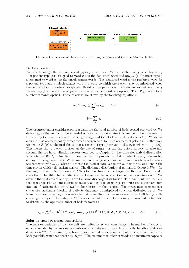
4.1. OPTIMISATION PROBLEM CHAPTER 4. SOLUTION APPROACH

Figure 4.3: Overview of the care unit planning decisions and their decision variables

Decision variablesWe need to assign the various patient types j to wards w. We define the binary variables assj,w(1 if patient type j is assigned to ward w) as the dedicated ward and misj,w (1 if patient type jis assigned to ward w) as the misplacement wards. The dedicated ward is the preferred ward fora patient type and a misplacement ward is a ward to which the patient may be misplaced whenthe dedicated ward reaches its capacity. Based on the patient-ward assignment we define a binaryvariable uw (1 when ward w is opened) that states which wards are opened. Then Ψ gives the totalnumber of wards opened. These relations are shown by the following equations.

bigM · uw ≥∑j

assj,w ∀w (4.8)

Ψ =∑w

uw (4.9)

The resources under consideration in a ward are the total number of beds needed per ward w. Wedefine mw as the number of beds needed on ward w. To determine this number of beds we need toknow the patient-ward assignment assj,w,misj,w and the block scheduling decision bj,s. We defineφ as the misplacement policy, which states decision rules for misplacement of patients. Furthermorewe denote Ej(n) as the probability that a patient of type j arrives on day n, in which n ∈ −1, 0.This means that a patient arrives on the day of surgery or the day before surgery, to take intoaccount the pre hospitalisation process described in Chapter 2. The time slot arrival distributionis denoted as W j

n(t). This distribution denotes the probability that a patient type j is admittedon day n during time slot t. We assume a non-homogeneous Poisson arrival distribution for acutepatients with rate λj,d,t, where j denotes the patient type, d the arrival day of the week and t thetime slot in which this patient arrives. The discharge distribution of patients is denoted P j(n) forthe length of stay distribution and M j

n(t) for the time slot discharge distribution. Here n and tstate the probability that a patient is discharged on day n or at the beginning of time slot t. Weassume that patients of one type have the same discharge distribution. The last inputs we need arethe target rejection and misplacement rates, χ and η. The target rejection rate states the maximumfraction of patients that are allowed to be rejected by the hospital. The target misplacement ratestates the maximum fraction of patients that may be misplaced to a non dedicated ward. Weintroduce these target rejection rates to make sure that our resources are utilised efficiently whileensuring quality care for patients. We have defined all the inputs necessary to formulate a functionto determine the optimal number of beds in ward w:

mw = f bedsw (b,bM,bA,assw,misw, φ,C,CM,CA,E,W, λ,P,M, χ, η) ∀w (4.10)

Solution space resource constraintsThe decision variables of the care unit are limited by several constraints. The number of wards toopen is bounded by the maximum number of wards physically possible within the building, which wedefine as Ψmax. Furthermore, each ward has a limited capacity in terms of the maximum number ofbeds possible, which we denote by Mmax

w . The maximum number of wards and maximum capacity

28

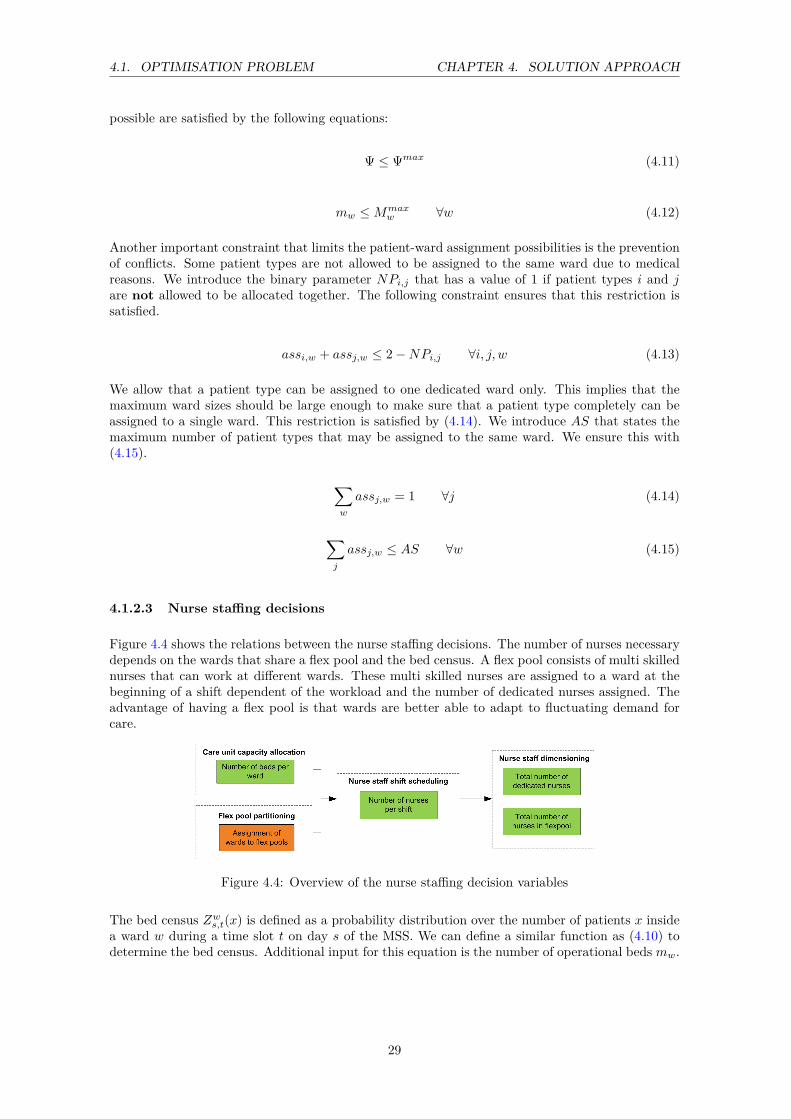
4.1. OPTIMISATION PROBLEM CHAPTER 4. SOLUTION APPROACH

possible are satisfied by the following equations:

Ψ ≤ Ψmax (4.11)

mw ≤Mmaxw ∀w (4.12)

Another important constraint that limits the patient-ward assignment possibilities is the preventionof conflicts. Some patient types are not allowed to be assigned to the same ward due to medicalreasons. We introduce the binary parameter NPi,j that has a value of 1 if patient types i and jare not allowed to be allocated together. The following constraint ensures that this restriction issatisfied.

assi,w + assj,w ≤ 2−NPi,j ∀i, j, w (4.13)

We allow that a patient type can be assigned to one dedicated ward only. This implies that themaximum ward sizes should be large enough to make sure that a patient type completely can beassigned to a single ward. This restriction is satisfied by (4.14). We introduce AS that states themaximum number of patient types that may be assigned to the same ward. We ensure this with(4.15).

∑w

assj,w = 1 ∀j (4.14)

∑j

assj,w ≤ AS ∀w (4.15)

4.1.2.3 Nurse staffing decisions

Figure 4.4 shows the relations between the nurse staffing decisions. The number of nurses necessarydepends on the wards that share a flex pool and the bed census. A flex pool consists of multi skillednurses that can work at different wards. These multi skilled nurses are assigned to a ward at thebeginning of a shift dependent of the workload and the number of dedicated nurses assigned. Theadvantage of having a flex pool is that wards are better able to adapt to fluctuating demand forcare.

Figure 4.4: Overview of the nurse staffing decision variables

The bed census Zws,t(x) is defined as a probability distribution over the number of patients x insidea ward w during a time slot t on day s of the MSS. We can define a similar function as (4.10) todetermine the bed census. Additional input for this equation is the number of operational beds mw.

29

4.1. OPTIMISATION PROBLEM CHAPTER 4. SOLUTION APPROACH

We do not need the target rejection and misplacement probabilities. The function to determine thebed census is given below:

Zws,t(x) = fCensus(b,bM,bA,assw,misw, φ,C,CM,CA,E,W, λt,P,M(t),mw) ∀w, s, t(4.16)

We first discuss the decision variables related to nurse staffing. Next, we introduce the variousresource constraints we consider.

Decision variablesWe need to determine which wards share the same flex pool. We denote flexf,w as the binaryvariable that denotes whether ward w uses flex pool f . Once the flex pool assignment is madeand the bed census Zws,t(x) for each ward is known we determine the optimal number of nurses interms of dedicated, nded, and flexible, nflex, staff. To determine the number of nurses necessarywe introduce target service levels that prevent that the workload for nurses gets too high and thepatients’ safety cannot be guaranteed any more. We introduce the patient nurse ratio rws,τ thatspecifies how many patients a nurse can care for during each shift τ on day s assigned on ward w.A patient nurse ratio of two specifies that for every two patients at least one nurse is necessary.We distinguish two types of desired service levels. The target overall service level α denotes thefraction of the time that the number of patients on a ward does not exceed the number of nursesstaffed times the patient nurse ratio. An overall service level of 95% states that one in twenty timeslots the nurse coverage may be insufficient. The minimum service level β states the minimumfraction of patients per time slot that should be covered by the staffed number of nurses times thepatient-nurse ratio. Futhermore we introduce γ which states the fraction of nurses on a ward thatshould be dedicated. The bed census in combination with the flexpool-ward assignment and thetarget nurse service levels are used as inputs for the following function to determine the number ofnurses in a flex pool and the number of dedicated nurses per ward.

(ndedw,s,t, nflexf,s,t) = fNurses(Zws,t, f lexf,w, α, β, γ, rw

s ) ∀w, f, s, t, (4.17)

The last step is to determine the total amount of FTE in terms of dedicated and flexible nurses.We do this by taking the sum of all dedicated nurses per ward and all flexible nurses per flex pool.

nded =∑w

∑s

∑t

ndedw,s,t (4.18)

nflex =∑f

∑s

∑t

nflexf,s,t (4.19)

Solution space resource constraintsWe define several quality constraints that limit the solution space. A nurse needs specialised trainingto treat a patient type j. Therefore it is not realistic that each nurse in a flex pool is qualified totreat all different patient types. We denote the binary parameter NFf,j that is 1 if a nurse fromflex pool f is not skilled to treat patient type j. Then (4.20) makes sure that only skilled nursesare assigned to patients they can care for.

assj,w + flexf,w ≤ 2−NFf,j ∀f, j, w (4.20)

We assume that a ward can only be assigned to one flex pool. Assigning more flex pools will notonly give a larger solution space but also complicates the situation from an operational perspective.How are hospital managers on an operational level going to decide the number of nurses needed per

30

4.1. OPTIMISATION PROBLEM CHAPTER 4. SOLUTION APPROACH

ward when they have the possibility to choose from multiple flex pools? To satisfy this we define:

∑f

flexf,w = 1 ∀w (4.21)

4.1.3 Optimisation objective

Section 4.1.2 gives the mathematical link between the decision variables and constraints of theplanning decisions. For each resource and patient case mix we define cost parameters to evaluatethe total costs. Based on these cost parameters we formally define the objective of this research:

min∑

j

F patientj · xj+∑rFnonrenewabler ·Ωr+FFTEd·nded+FFTEf ·nflex+

∑wFwardw ·uw+F bed·mw

In this objective function various cost parameters are present. We explain each parameter briefly:

• Revenue per patient type (F patientj ): Revenue or cost of a patient type j. When therevenues of a patient type j are higher than the costs this value is negative. We only considerpatient specific costs that are not accounted for by the other cost parameters. The resourcespecific costs per day are included in the revenue of a patient type.

• Non renewable resource costs per year (Fnonrenewabler ): The costs of investing in nonrenewable resources. For example the number of ORs and X-ray machines. This includesdepreciation costs.

• Cost of one dedicated nurse in FTE per year (FFTEd): Cost of one FTE of a dedicatednurse per year.

• Cost of one flexible nurse in FTE per year (FFTEf ): Cost of one FTE of a nurseassigned to a flex pool per year. Because nurses in a flex pool have extra skills and educationthis cost parameter may differ from FFTEd.

• Fixed costs to open a ward per year (Fwardw ): Fixed costs to open ward w per year.These fixed costs consist of overhead, depreciations and supporting staff other than nurses.

• Fixed costs of a bed per year (F bed): The fixed costs to place a bed in a ward.

Based on the stated cost parameters we can evaluate the objective function for various resourceconfigurations. In Section 4.2 we explain our decomposition approach to make the resource capacityplanning decisions and to minimise the objective function.

4.1.4 Performance indicators

To measure the performance of the block scheduling decision on the resource utilisation we definethe non renewable OR resource utilisation given by (4.22).

ORresutilr = Ωr · S∑s

∑j

REj,r · bj,s + 1

2REMj,r · bMj,s +REAj,r · bAj,s

∀r (4.22)

To measure the performance of resources in the clinical wards we first determine the average bedcensus of each time slot. The average bed census Zws,t is given by (4.23).

Zws,t =mw∑x=1x · Zws,t(x) ∀s, t, w (4.23)

31

4.2. DECOMPOSITION APPROACH CHAPTER 4. SOLUTION APPROACH

Once we know the average bed census we can define the operational bed utilisation by taking thesum of the average bed census for each time slot and day of the MSS:

Bedutilw =

∑s

∑tZws,t

S · T ·mw∀w (4.24)

The performance indicators for the number of nurses are given by the realised α and β service levelsfor which we use the mathematical notation as given by Burger [9].

4.2 Decomposition approach

This section describes our solution approach to solve the optimisation problem defined in Section4.1. We use a decomposition approach because the solution space is extremely large and the re-lationships between variables are complex and non linear. Figure 4.5 shows the different stepsof our decomposition approach. In the following sections we will discuss each step in more detail.Throughout this section we assume that the reader has taken knowledge of the variables and param-eters that are introduced in Section 4.1. For a complete overview of the variables and parametersused in this section we refer to Appendix A.

Figure 4.5: Decomposition approach to solve the optimisation problem

4.2.1 Set number of blocks and length of MSS

We set the number of patients per type, xj , to treat and the length of the MSS, S, as inputparameters. We derive the ratio between full, morning and afternoon blocks from historical data.From xj and S we then can determine the number of full blocks, Bnormj , morning blocks, Bnorm,Mj ,and afternoon blocks, Bnorm,Aj , that we need to schedule.

4.2.2 Block scheduling in the OR and patient-ward assignment

In this step we create a block schedule and assign patient types to wards. From Section 4.2.1 weknow the number of blocks to schedule and the length of the MSS.

The block scheduling decision can be characterised as a bin packing problem, in which a list ofitems is assigned to a minimum number of bins. Surgery blocks can be seen as the items and thenumber of ORs to open as the minimum number of bins. The patient ward-assignment is defined inthe literature as a bin packing problem with conflicts. In this case we want to assign each patienttype (items) to a ward (bins) without exceeding maximum capacity and violation of the constraintthat some patient types cannot be allocated to the same ward.

The patient-ward assignment and the block scheduling decision are interrelated. Both decisionstogether are main contributors to the resource usage inside a ward. Therefore it is not clear whichdecision should be taken first in a decomposition. Within the literature bin packing problems are

32

4.2. DECOMPOSITION APPROACH CHAPTER 4. SOLUTION APPROACH

defined as Integer Linear Programs (ILP) and can be solved with commercial software like CPLEX.By nature bin packing problems are NP-hard, which means they are hard to solve when instancesget too large. When instances get too large we can use an taboo search or graph theory algorithmto solve the bin packing problem with conflicts, see for example [22] and [25].

We formulate an ILP that combines the block scheduling in the OR and the patient ward assign-ment. The objective of the block scheduling decision and the patient ward assignment consists ofminimisation of:

• Number of non renewable resources Ωr.

• Number of Wards Ψ to open.

• Expected number of beds mµw on a ward.

• Expected number of nurses nµw,s,τ needed on ward w on day s during shift τ

When we minimise the number of beds and the number of nurses needed per ward, we automaticallylevel the workload inside the wards. Minimisation of these resources is translated into the followingobjective function:

min∑

r

κnonrenewabler · Ωr +∑w

κwardsw · uw + κbeds ·mµw + κnurses ·

∑s

∑τ

nµw,s,τ

(4.25)

In this objective function the various κ values determine the weight factors of the resources. Wecan choose for example to use the cost parameters defined in Section 4.1.3 to determine the valuesfor κ.

Let us define the decision variables bj,s,w, bMj,s,w, bAj,s,w as the number of surgery blocks of patienttype j assigned to ward w and scheduled on day s. The prefixes M and A make the distinctionbetween morning and afternoon blocks. We combine the patient-ward assignment and the blockscheduling decision into one decision variable because these are interrelated and multiplication ofvariables causes a non linear problem. The downside of this approach is that the number of variablesrapidly increases which makes it harder to solve this ILP to optimality. To make sure that we assignall blocks that we set in Section 4.2.1 of our decomposition approach the following three equationsshould be satisfied:

∑s

∑w

bj,s,w = BNormj ∀j (4.26)

∑s

∑w

bMj,s,w = BNorm,Mj ∀j (4.27)

∑s

∑w

bAj,s,w = BNorm,Aj ∀j (4.28)

(4.29) and (4.30) ensure that the number of non renewable OR resources are set when a block isscheduled on a given day.

∑j

∑w

REj,r · bj,s,w +REMj,r · bMj,s,w ≤ Ωr ∀r, s (4.29)

∑j

∑w

REj,r · bj,s,w +REAj,r · bAj,s,w ≤ Ωr ∀r, s (4.30)

33

4.2. DECOMPOSITION APPROACH CHAPTER 4. SOLUTION APPROACH

When a surgery block of patient type j is scheduled on day s and assigned to ward w, (4.31) ensuresthat the variable assj,w becomes 1 for this patient-ward combination. The parameter AS limitsthe maximum number of patient types that can be assigned to the same ward. (4.32) ensuresthat a patient type is only assigned to one ward. (4.33) ensures that the constraint related to themaximum number of non renewable OR resources present is not violated. (4.34) and (4.35) satisfythat a ward is opened when a patient type is assigned to it and (4.36) ensures that patient typeswith conflicts are not allocated to the same ward.

∑s

bj,s,w + bAj,s,w + bMj,s,w ≤ bigM · assj,w ∀j, w (4.31)

∑w

assj,w = 1 ∀j (4.32)

Ωr ≤ Ωmaxr ∀r (4.33)

AS · uw ≥∑j

assj,w ∀w (4.34)

Ψ =∑w

uw (4.35)

assj,w + assi,w ≤ 2−NPi,j ∀j, i, w (4.36)

∑j

Lmaxj∑

n=−1Gj(n) · E[Cj ] · bj,s−n,w + E[CMj ] · bMj,s−n,w + E[CAj ] · bAj,s−n,w+

∑j

Lmaxj∑n=0

Gj(n) · λj,s−n · assj,w ≤ mµw ∀s, w

(4.37)

We define (4.37) to calculate the expected number of beds on a ward, mµw. This constraint is based

on the ILP formulation given by Adan et al. [3]. The first part of (4.37) consists of the expectednumber of elective patients and the latter part states the number of acute patients. Gj(n) states theprobability that a patient is still present inside the hospital on day n. Where n ∈ −1, . . . , Lmaxcounts the number of days before or after surgery, with surgery on day n = 0. The demand thatresults from a scheduled surgery block is calculated based on the average number of patients insidea block. The number of acute patients of type j that arrive on day s − n is given by λj,s−n. Todetermine the expected maximum number of beds needed we take the sum over all patient types jand the maximum length of stay of a patient type j and calculate the number of beds occupied oneach day, s, of the MSS. To take the pre operative stay into account we take the sum from n = −1.Because it occurs that the LOS of some patients is longer than the MSS we use the convention thatthe subscript s − n should be treated as modulo S. This means that day -1 is the same as dayS−1. The maximum number of beds physically possible on a ward is given by MMax

w . In (4.37) wecalculate the maximum number of expected beds needed. In the real world there is some variationin beds. To make sure that we take this variation into account we define the stochastic capacityscale factor, ε, that prevents us from exceeding the maximum capacity.

mµw ≤ ε ·MMax

w (4.38)

34

4.2. DECOMPOSITION APPROACH CHAPTER 4. SOLUTION APPROACH

To estimate the required number of nurses per day we define a similar equation as for the estimatednumber of beds. We denote the estimated number of nurses needed by Nw,s,τ . The number ofnurses needed depends on the number of patients present and the time of the shift τ . In 4.39 wedenote rj,τ as the nurse care ratio that specifies how many patients of type j a nurse can care for.

∑j

rj,s,τ

Lmaxj∑

n=−1Gj(n) · E[Cj ] · bj,s−n,w + E[CMj ] · bMj,s−n,w + E[CAj ] · bAj,s−n,w+

∑j

rj,s,τ

Lmaxj∑n=0

Gj(n) · λj,s−n · assj,w ≤ nµw,s,τ ∀s, w, τ

(4.39)

Elective surgery only takes place on working days so we need to make sure that no blocks areassigned to weekend days. We satisfy this requirement with the following constraints. We assumethat the length of the MSS is a multiple of seven days and that Monday is day 1.

bj,s,w = 0 and bj,s+1,w = 0 s = 6 + 7 · (h− 1) h = 1 . . . (S7 ) j, w, s

bMj,s,w = 0 and bMj,s+1,w = 0 s = 6 + 7 · (h− 1) h = 1 . . . (S7 ) j, w, s

bAj,s,w = 0 and bAj,s+1,w = 0 s = 6 + 7 · (h− 1) h = 1 . . . (S7 ) j, w, s

(4.40)

To finalise our ILP we define the following integer constraints:

bj,s,w, bMj,s,wb

Aj,s,w, n

µw,s,τ ,m

µw,Ψ,Ωr ∈ 0, 1, 2... (4.41)

assj,w, uw ∈ 0, 1 (4.42)

4.2.3 Access Time model by Kortbeek et al.

In section 4.2.2 we propose a method to create a block schedule and assign patients to wards. Ouroptimisation problem in Section 4.1 states that the outcome of the block scheduling decision shouldsatisfy the desired target OR access time service level. The access time service level is a function ofseveral inputs and given by (4.6). To evaluate the access time service level we use the methodologyproposed by Kortbeek et al. [19] for this function. First, we summarise the model of Kortbeek etal. [19]. Next, we discuss how we use this model to determine the realised OR access time servicelevel.

Kortbeek et al. propose[19] a methodology to design cyclic appointment schedules for outpatientclinics with scheduled and unscheduled arrivals. Their method is based on an algorithm that linkstwo models. The first model evaluates the access time for scheduled arrivals and the second modelevaluates the day process of scheduled and unscheduled arrivals. The access time is evaluatedgiven the distribution of the number of appointment requests per day and the number of availableappointments slots per cycle. A cycle is a fixed time period of several days that is continuouslyrepeated. For each cycle the backlog distributions are determined. Backlog is defined as the numberof appointment requests that have been made while the actual appointment has not yet taken place.Based on the derivation of moment generating functions the steady state transition probabilitiesfor the backlog at the start of each day in the cycle are determined. Based on these transition

35

4.2. DECOMPOSITION APPROACH CHAPTER 4. SOLUTION APPROACH

probabilities it is possible to derive the expected access time service level.

The methodology proposed by Kortbeek et al. needs the distribution of the number of appointmentrequests per day and the number of available planning slots per cycle. When we translate thisanalogy to the access time of the OR we need to know the distribution of the number of surgeryrequests per day and the capacity of a surgery block. The model of Kortbeek assumes deterministicappointment durations. To model the capacity of a surgery block we use the expected number ofpatients in a surgery block, denoted E[Cj ]. We derive the distribution of the number of surgeryrequests per day from historical data. When the access time service level is below our predefinedtarget we can adjust the assignment of blocks to days or we need to increase the number of blocksscheduled. Our ILP, described in Section, 4.2.2 is designed in such a way that it levels the expectednumber of beds needed on a ward. This means that the surgery blocks are most likely evenly dis-tributed over the MSS cycle. It is therefore reasonable to expect that changing the block schedulingdecision will only yield small improvements in the access time service level. Increasing the numberof blocks that are scheduled provides better results.

4.2.4 Hourly Bed Census model by Smeenk et al.

The hourly bed census is based on the Master Surgical Schedule and the patient-ward assignment.To determine the number of beds needed on a ward w we defined (4.10). For this function we canuse the model developed by Smeenk et al. [29] which provides the number of beds needed per wardgiven the target rejection and misplacement rates. In this section we provide a brief summary ofthe model developed by Smeenk. For more detailed information regarding the model of Smeenk,we refer to the thesis of Smeenk [29].

Figure 4.6 shows the three consecutive steps to obtain the bed census per ward. First, the demandof elective patients is determined. Next, the demand resulting from the arrival of acute patients iscalculated. In the last step both demand distributions are combined. We discuss each step in moredetail.

Figure 4.6: Overview of the different steps to obtain the bed census on a ward

Elective steady state: First, the demand for beds at a ward resulting from a single surgery blockis calculated. This is done for each surgery block of each patient type. In the next step a single MSSis considered in isolation in which multiple surgery blocks are present. The single cycle demandis created by means of discrete convolutions, because patients from a block scheduled on previousdays are still recovering in a ward when new patients arrive. The last step is to consider multipleoverlapping MSS cycles by taking discrete convolutions of the single cycle demand.

Acute Steady State: The steady state demand for acute patients is determined in a similar wayas for elective patients. The first step is to determine the influence of a single acute patient typethat arrives on a day d. Next, the influence of multiple patient types in a cycle is considered.The cycle length for acute patients is R days. The steady state cycle is calculated with discreteconvolutions of the single patient types. The final step is to consider multiple overlapping cyclesby taking discrete convolutions of the single cycle demand. We need discrete convolutions becausepatients from a previous cycle may still be recovering in the next cycle(s).

36

4.2. DECOMPOSITION APPROACH CHAPTER 4. SOLUTION APPROACH

Ward Steady State: Both steady state distributions are combined by discrete convolutions toobtain the steady state ward demand distribution. This demand distribution states the probabilitythat x patients are present on day s during time slot t on ward w.

The method proposed by Smeenk also has the possibility to misplace patients between multiplewards given predefined control rules. Given the number of beds on a ward the model computesthe realised rejection and misplacement rates. To determine the number of beds needed per wardwe initially set the number of beds at a predefined value. Then, we evaluate the correspondingrejection and misplacement rates for this number of beds and compare this with our target rates. Ifthe realised rates are above the targets we need to increase the number of beds. When the realisedrates are below the targets we decrease the number of beds. We do this iteratively until we havereached the minmial number of beds for which the targets are satisfied. For the exact mathematicalformulation of the misplacement policy and the rejection and misplacement rates we refer to thethesis of Smeenk [29].

4.2.5 Flex pool decisions

In this section we explain our procedure to evaluate all flex pool assignment possibilities amongthe different wards. We use the model of Burger [9] to determine the number of dedicated nursesper ward and the number of nurses within a flex pool. This model needs as input the wards thatshare the same flex pool and the bed census derived from the model of Smeenk. Section 4.2.6discusses the model of Burger in detail. Because the number of flex pools is low and the numberof wards that share the same flex pool is limited we can use total enumeration to evaluate all flexpool combinations. In this section we describe our four step method that makes use of the modelof Burger. We illustrate our method by means of an example.

1. Set number of flex pools that can be used.

2. Create a set of all combinations of 2 to Ψ wards sharing a flex pool, in which Ψ denotes thenumber of wards opened. Remove combination of wards that are not allowed to share thesame flex pool together because the nurses are not trained to treat all their patient types.

3. For each combination in the set determine the number of dedicated nurses needed and thenumber of nurses within a flex pool. We use the model of Burger to do this.

4. Select the combination that minimises the number of nurses needed.

Now we give our example:

1. We set the number of flex pools used at two. Let us consider four wards, of which ward 1 andward 2 cannot share the same flex pool.

2. We compute all possible combinations in which two, three or four wards share the same flexpool. We remove the combinations in which ward 1 and ward 2 share the same flex pool.

3. For each combination determined in step 2 we calculate the number of dedicated nurses perward and the number of nurses in a flex pool.

4. We select the combination that minimises the number of nurses needed. We have the optionto have one flex pool for three wards or two flex pool of two wards. One flex pool of fourwards is not an option because ward 1 and ward 2 can not share the same flex pool.

4.2.6 Nurse staffing model by Burger et al.

The number of dedicated nurses and flexible nurses needed per shift depends on the demand forbeds by patients and the flex pool ward assignment. Dedicated nurses are always assigned to the

37

4.3. SOFTWARE IMPLEMENTATION CHAPTER 4. SOLUTION APPROACH

same ward and flexible nurses are assigned to the ward that has the highest shortage of nurses atthe start of a shift. In Section 4.1 we defined (4.17) to calculate the optimal number of nursesneeded given two service levels. We can use the model of Burger [9] et al. to determine the optimalnumber of dedicated and flexible nurses per shift. In this section we briefly summarise the modelof Burger. For more detailed information regarding the model of Burger, we refer to the thesis ofBurger [9]

Burger assumes that shifts are non-overlapping and nurses only work full shifts. Furthermore,a nurse can only be assigned to one ward during a shift. The model of Burger consists of thedetermination of three solution bounds and uses two target service levels and a minimum fractionof dedicated nurses per ward. The overall service level α states the fraction of the time that thenumber of patients on a ward does not exceed the number of nurses staffed times the patient nurseratio, rws,τ . The minimum service level β states the minimum fraction of patients per time slot thatare covered by the staffed number of nurses times the patient-nurse ratio. The first bound solution(Non Flexible) is calculated while considering no flexibility. This means that the first bound givesthe optimal number of dedicated nurses needed per shift and ignores the use of flex pools. Thesecond bound solution (Lower Bound flexible) considers the use of flexible nurses but relaxes theconstraint that these nurses need to be assigned to one ward for the whole shift. The third boundsolution (Upper Bound flexible) is computed based on the maximum number of patients that arepossibly present on a ward during a shift. The maximum number of patients present during a shiftcannot be derived from the bed census so these are determined in an alternative way given theMSS and the patient arrival and discharge distributions [9]. Burger uses decision rules to select theoptimal number of dedicated and flexible nurses given the solutions of the three bounds. Figure 4.7summarises the steps mentioned above.

Figure 4.7: Overview of the different steps to obtain the number of dedicated nurses per ward andthe number of flexible nurses inside a flex pool per shift per day

4.3 Software implementation

The mathematical relationships between the various variables and the objective function from Sec-tion 4.1 are programmed in Delphi. For the functions (4.2.3), (4.2.4), and, (4.2.6) we use the modelsof Kortbeek, Smeenk, and Burger to evaluate the access time, determine the number of beds andthe number of nurses required. These models were already programmed in Delphi so we had tolink them together and make minor adjustments. We integrated these into one large evaluation andoptimisation tool. The class diagram of our Delphi program is shown in Appendix D.

We formulated the ILP in a program called OmpShell and solved it with CPLEX. OmpShell isa program developed by Erwin Hans which makes it easy to input an ILP in the mathematicalnotation. The output of the ILP can easily be imported into our evaluation/optimisation tool andthen be processed further to evaluate the effect on the resource usage in the inpatient care chain.

The programmed models of Smeenk and Burger have some limitations due to computational com-plexity which limits our solution space. We briefly summarise these limitations:

38

4.4. VERIFICATION & VALIDATION CHAPTER 4. SOLUTION APPROACH

• The maximum number of wards that can exchange patients is two. This means that a patientcan only be misplaced to one other ward. It is not easy to extend this to more than twowards.

• The misplacement and rejection rates that the model of Smeenk computes do not provideaccurate values. To resolve this, we neglect the possibility of misplacements. To determinethe optimal number of beds per ward we take the 90% demand percentile of the bed census.Within the AMC the model of Smeenk is still improved and an update can easily be integratedinto our optimisation tool.

• The maximum number of wards that can share a flex pool is limited to two. It is not easy toextend this to more than two wards.

4.4 Verification & validation

In Section 4.4.1 we discuss the verification of our model. Section 4.4.2 describes the process ofvalidation.

4.4.1 Verification

Verification is concerned with determining whether our model has been correctly translated intoan computer program [20]. To verify whether our model does not contain any bugs or errors wechecked the output of the ILP solution to verify whether no constraints are violated. To test if weintegrated the models of Kortbeek, Smeenk and Burger correctly, we created single data files thatcontain the same input as in our integral model. The single output of the models show exact thesame results as used in our integrated tool. This indicates that we combined the models correctly.

4.4.2 Validation

Validation is the process of determining whether a model is an accurate representation of the realworld, for the particular objectives of this study [20]. Validation of our proposed method is difficultdue to two reasons. First, the current situation is highly diverse and not standardised. Eachdepartment in our case study has different ways to plan and schedule patients which is impossibleto simulate with our model. This lack of standardisation makes it difficult to incorporate this intoour model. Second, our modelling approach aims at optimisation which is completely different fromthe current practice. Therefore it is not possible to use our model to obtain the same results as inthe current practice. To validate our model we propose a theoretical simulation study in which weuse the outcomes of our solution approach and compare this with real data.

4.5 Conclusions

In this chapter we formulated our research objective as a mathematical optimisation problem. Tosolve this optimisation problem we propose a decomposition approach optimise the resource usagein the inpatient care chain while considering various decisions. To reduce modelling complexity wehad to make a few simplifications compared to the current situation. We propose an ILP to makethe patient-ward assignment and to create a master surgical schedule. We used various existingmodels from literature to determine and optimise the downstream resources requirements in termsof beds and nurses required per nursing ward. Compared to the various literature related to resourcecapacity planning in the OR department and the nursing wards this is one of the first researchesthat focuses on decisions and optimisation that affects the whole chain.

39

Chapter 5

Computational results

In this chapter we demonstrate the performance of the approach developed in Chapter 4 by con-ducting several experiments. Section 5.1 describes our data gathering approach to obtain the valuesof relevant distributions and parameters. In Section 5.2 we clarify which parts of our decompositionapproach we exclude when we conduct our experiments. Section 5.3 discusses our experimentalset-up. Section 5.4 describes our experimental approach to model the current situation and thevarious experiments we perform. Section 5.5 shows the results of the experiments we conduct. Weend this chapter with conclusions in Section 5.6.

5.1 Data gathering

We obtain data from the various systems present in the AMC to test our solution approach. Thesurgery, admission and discharge distributions are gathered from two separate systems: Locati andOK-Plus. Locati contains all the admission and discharge data of the patients that reside on award. OK-plus contains all data from the surgeries. There is no direct link between an admissionand a surgery so we have to perform several steps to create the relevant data sets. Appendix Bdiscusses these steps in more detail and provides the relevant figures for our case study. Due tothe poor quality of the data, we had difficulties matching admitted patients to an accompanyingscheduled surgery block, since we consider patients who do not have had an surgery as acute.This had as result, that 51% of the total patients considered in this case study are of the acutepatient type, which is remarkable because we are considering the surgical department in whichmost admissions are caused by surgical procedures. Relevant data regarding the distribution of thenumber of surgery requests for each patient type was not possible to obtain within the availabletime frame of this research. We had various conversations with several departments in the AMCto obtain the relevant cost parameters present in our objective function (Section 4.1.3). Moredetailed information regarding these conversations and a derivation of the required cost parametersis provided in Appendix C.

5.2 Demarcation experiments

In the experiments we conduct in this chapter we limit ourselves compared to the full potential ofour decomposition approach, which is described in Section 4.2. We exclude:

• Access time service level: As stated in Section 5.1 we do not have available data regardingthe distribution of surgery requests per patient type.

41

5.3. EXPERIMENTAL SET-UP CHAPTER 5. COMPUTATIONAL RESULTS

• Rejection and misplacement rates: We do not consider evaluation of the rejection andmisplacement rates as stated in Section 4.3. The realised model in Delphi of Smeenk does notprovide accurate values for these rates.

• Costs and revenues per patient type: We do not have available data concerning the costsand revenues per patient type, which we need to evaluate the effect of a chosen patient casemix on the total costs. Therefore we focus on minimisation of the total resource costs for agiven patient case mix.

• Minimisation of expected number of nurses in the ILP:We programmed the constraint(4.39) that corresponds to the expected number of nurses required per shift per day in theprogram Ompshell, but due to the large number of variables (over 3000) the program wouldnot run.

5.3 Experimental set-up

Figure 5.1 shows the two computer programs we developed to perform our experiments. We solveour ILP, described in Section 4.2.2 for the creation of a block schedule and the patient-ward assign-ment, with the program OmpShell that uses CPLEX. The integrated tool consists of the modelsdeveloped by Kortbeek (Section 4.2.3), Smeenk (Section 4.2.4), and Burger (Section 4.2.6) in Del-phi to determine the number of beds and nursing staff needed, and to derive several performanceindicators.

Figure 5.1: Overview of the two models we use

We perform our experiments on a computer with Windows XP professional, with an Intel Core2 Duo 3.00 GHz processor and 4 GB of available RAM. We use CPLEX version 12.1 and Delphiversion XE. For all experiments we conduct we use the default parameters stated in Table 5.1. Weexplicitly mention it when we deviate from these parameters. Table 5.2 contains the managerialoutput we obtain for each experiment. We measure the total number of nurses in our integratedDelphi model in Full Time Employee (FTE).

Parameter Value Parameter ValueS Length of MSS 28 ε Bed capacity scale factor 0.7T Number of time slots 24 κnonrenewableOR Weight of an OR 500,000T Number of shift types 3 κbeds Weight of a bed 9,000χ Target rejection rate - κwards Weight of a ward 1,250,000η Target misplacement rate - FFTEd Cost of a dedicated nurse 50,000α Target overall service level 0.95 FFTEf Cost of a nurse in flex pool 50,000β Target minimum service level 0.80 Max runtime ILP 30 minγ Minimum fraction of dedicated nurses per ward 0.66

Table 5.1: Default parameter values used in our experiments

42

5.4. EXPERIMENTAL DESIGN CHAPTER 5. COMPUTATIONAL RESULTS

ILP solution method Integrated Delphi modelGeneral General

Number of ORs to open Expected number of patients treated per yearNumber of wards to open OR utilisationRuntime Total number of bedsIntegrality gap Total number of nurses

Total number of flex pools usedTotal number of dedicated nursesTotal number of nurses per flex poolRuntime model SmeenkRuntime model Burger

Ward specific Ward specific

Expected number of beds Min number of beds based on 90%th demand percentilePatient-ward assignment Max number of beds based on 90%th demand percentile

Average bed utilisationTotal FTE dedicated nurses per yearFlex pool-ward assignmentRealised average overall and minimum service levels peryear

Table 5.2: Managerial output of our experiments

5.4 Experimental design

We have structured our experimental design as follows. In Section 5.4.1 we determine the managerialoutput described in Table 5.2 given the resource capacity planning decisions made in the currentsituation. In Section 5.4.2 we systematically show the effects of the resource usage in the inpatientcare chain for the various optimisation steps of our decomposition approach. In Section 5.4.3 weconsider two types of scenarios that affect the LOS distribution and the number of acute patienttypes on which we have limited influence. We continue in Section 5.4.4 with a sensitivity analysis ofthe weighing factors used in the ILP and of the various parameters used to determine the requirednumber of nurses. Section 5.4.5 concludes with alternative interventions, which consist of adaptingOR planning decisions and a different admission and discharge process.

5.4.1 Division B: Current situation

In our experiments we focus on the current situation of Division B (see Chapter 2 for detailedinformation). In 2012 the board of division B has decided to change the allocation of patient typesto wards, compared to the situation of 2011 described in Table 2.4. To take the actual situationof 2012 into account we assume the ward lay-out and patient-to-nurse ratios as described in Table5.3.

Patient-to-nurse ratioWard Patient type(s) Beds Nurses (FTE) Morning shift Evening shift Night shiftG5 Noord URO, VAA 31 25.5 5.0 5.0 10.0G6 Noord CHI, CHIss 27 27.7 4.0 6.0 8.0G6 Zuid CHI, CHIss, MZK 28 28.8 4.0 6.0 8.0G7 Noord TRA 24 24.0 4.5 4.5 9.0G7 Zuid ORT, CHP 28 21.8 5.0 8.0 10.0

Table 5.3: Overview of patient types assigned to the various wards in Division B 2012 and thepatient-to-nurse ratio for each ward (Source: [8]).

43

5.4. EXPERIMENTAL DESIGN CHAPTER 5. COMPUTATIONAL RESULTS

We need to make a few adjustments to be able to evaluate the situation of 2012 with our model.The AMC does not use a cyclic master surgical schedule which is needed for our model. To beable to compare our solution approach to the results of the current situation we select the blockschedule of the first four weeks of September 2010 and assume this is cyclic for the rest of the year.We choose the month September because there are no holidays in these weeks and these are thebusiest of the year. We consider a surgical specialty as one unique patient type. Our modellingapproach assumes that each patient type has its own surgery block. In the current situation surgicalshort stay patients (CHIss) undergo surgery in the same surgery blocks as general surgery patients(CHI). To model this, we assume that surgical short stay patients and general surgery patients arethe same patient type, which have the same admission, discharge, and LOS distribution. Anotherassumption in our model is that each patient type needs to be assigned to one ward. In the currentsituation the patient types surgery (CHI) and surgical short stay (CHIss) are assigned to two wards.To model this, we create two surgical patient types of which one patient type is assigned to wardG6 Noord and the other to ward G6 Zuid. We adapt the block scheduling in such a way that alleven blocks in the cycle of the general surgery type scheduled are assigned to ward G6 Noord andall uneven blocks to ward G6 Zuid.

5.4.2 Optimisation interventions

In this section we describe experiments to systematically obtain the effects of the various inter-ventions of our decomposition approach compared to the experiment of the current situation. InSection 5.4.2.1 we create a cyclic MSS which levels the expected number of beds. Section 5.4.2.2contains experiments regarding the patient-ward assignment. We continue in Section 5.4.2.3 withan experiment to determine the optimal flex pool configuration. Section 5.4.2.4 concludes with acombination of all optimisation steps.

For each experiment described in this section we use the default parameters from Table 5.1. Forthe planning decisions we use the settings stated in Table 5.4. When we deviate from these defaultsettings we will mention this explicitly.

Planning decisions Default settingsBlock scheduling decision 4-Weekly MSS based on September 2010Patient-ward assignment We use the assignment from Table 5.3Misplacement policy No misplacements are allowedFlex pool assignment No flex pools are used

Table 5.4: Default planning decisions used for optimisation experiments

5.4.2.1 Master Surgical Schedule

In this experiment we use our developed ILP method to create an MSS with a cycle length offour weeks. We set the maximum number of blocks to be scheduled equal to the number of blocksscheduled in the first four weeks of September 2010. We set the maximum number of beds possibleper ward equal to 50 to make sure that our optimal solution is not limited by insufficient numbersof beds. The resulting MSS is used as an input for our integral tool to evaluate the other resourceneeds.

Along with this experiment we also conduct an experiment to determine the run time of our ILP.Our ILP contains many variables that makes it difficult to obtain an optimal solution quickly. Tospeed up the process we choose to manually stop CPLEX after a fixed time period. To determine theappropriate running time value versus integrality gap we experiment with run times of 30 minutes,1 hour, 2 hours, 4 hours and 8 hours. We use the outcome of the running time experiment in allother experiments.

44

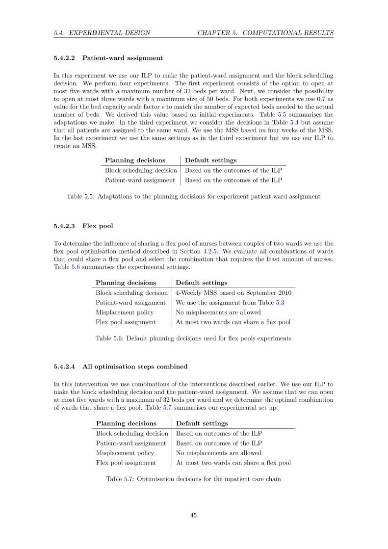
5.4. EXPERIMENTAL DESIGN CHAPTER 5. COMPUTATIONAL RESULTS

5.4.2.2 Patient-ward assignment

In this experiment we use our ILP to make the patient-ward assignment and the block schedulingdecision. We perform four experiments. The first experiment consists of the option to open atmost five wards with a maximum number of 32 beds per ward. Next, we consider the possibilityto open at most three wards with a maximum size of 50 beds. For both experiments we use 0.7 asvalue for the bed capacity scale factor ε to match the number of expected beds needed to the actualnumber of beds. We derived this value based on initial experiments. Table 5.5 summarises theadaptations we make. In the third experiment we consider the decisions in Table 5.4 but assumethat all patients are assigned to the same ward. We use the MSS based on four weeks of the MSS.In the last experiment we use the same settings as in the third experiment but we use our ILP tocreate an MSS.

Planning decisions Default settingsBlock scheduling decision Based on the outcomes of the ILPPatient-ward assignment Based on the outcomes of the ILP

Table 5.5: Adaptations to the planning decisions for experiment patient-ward assignment

5.4.2.3 Flex pool

To determine the influence of sharing a flex pool of nurses between couples of two wards we use theflex pool optimisation method described in Section 4.2.5. We evaluate all combinations of wardsthat could share a flex pool and select the combination that requires the least amount of nurses.Table 5.6 summarises the experimental settings.

Planning decisions Default settingsBlock scheduling decision 4-Weekly MSS based on September 2010Patient-ward assignment We use the assignment from Table 5.3Misplacement policy No misplacements are allowedFlex pool assignment At most two wards can share a flex pool

Table 5.6: Default planning decisions used for flex pools experiments

5.4.2.4 All optimisation steps combined

In this intervention we use combinations of the interventions described earlier. We use our ILP tomake the block scheduling decision and the patient-ward assignment. We assume that we can openat most five wards with a maximum of 32 beds per ward and we determine the optimal combinationof wards that share a flex pool. Table 5.7 summarises our experimental set up.

Planning decisions Default settingsBlock scheduling decision Based on outcomes of the ILPPatient-ward assignment Based on outcomes of the ILPMisplacement policy No misplacements are allowedFlex pool assignment At most two wards can share a flex pool

Table 5.7: Optimisation decisions for the inpatient care chain

45

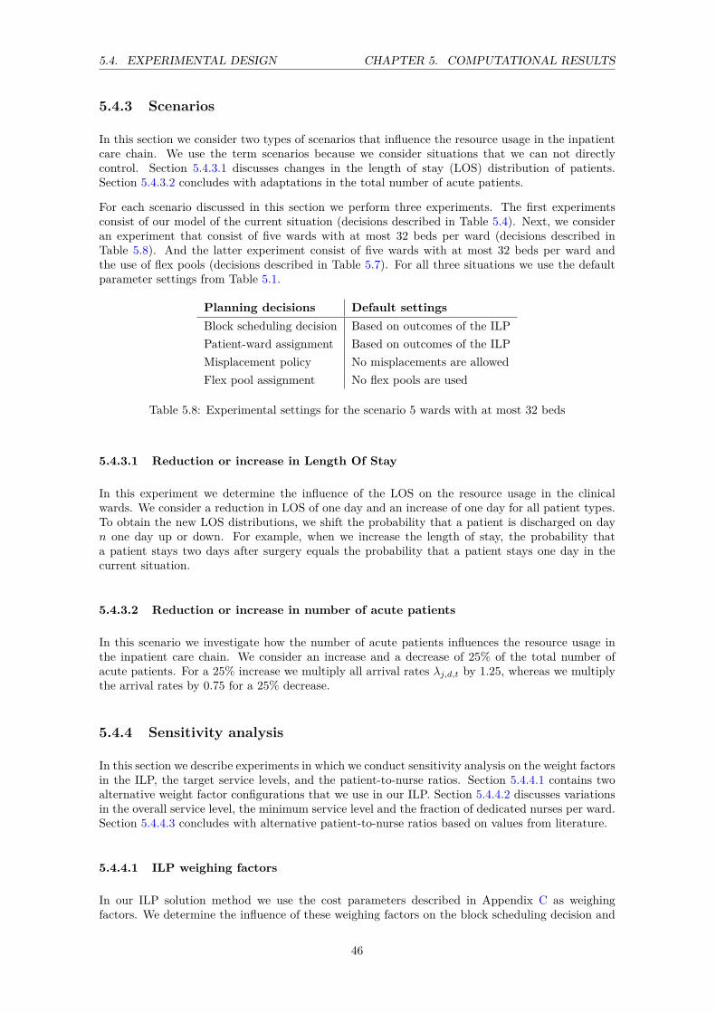
5.4. EXPERIMENTAL DESIGN CHAPTER 5. COMPUTATIONAL RESULTS

5.4.3 Scenarios

In this section we consider two types of scenarios that influence the resource usage in the inpatientcare chain. We use the term scenarios because we consider situations that we can not directlycontrol. Section 5.4.3.1 discusses changes in the length of stay (LOS) distribution of patients.Section 5.4.3.2 concludes with adaptations in the total number of acute patients.

For each scenario discussed in this section we perform three experiments. The first experimentsconsist of our model of the current situation (decisions described in Table 5.4). Next, we consideran experiment that consist of five wards with at most 32 beds per ward (decisions described inTable 5.8). And the latter experiment consist of five wards with at most 32 beds per ward andthe use of flex pools (decisions described in Table 5.7). For all three situations we use the defaultparameter settings from Table 5.1.

Planning decisions Default settingsBlock scheduling decision Based on outcomes of the ILPPatient-ward assignment Based on outcomes of the ILPMisplacement policy No misplacements are allowedFlex pool assignment No flex pools are used

Table 5.8: Experimental settings for the scenario 5 wards with at most 32 beds

5.4.3.1 Reduction or increase in Length Of Stay

In this experiment we determine the influence of the LOS on the resource usage in the clinicalwards. We consider a reduction in LOS of one day and an increase of one day for all patient types.To obtain the new LOS distributions, we shift the probability that a patient is discharged on dayn one day up or down. For example, when we increase the length of stay, the probability thata patient stays two days after surgery equals the probability that a patient stays one day in thecurrent situation.

5.4.3.2 Reduction or increase in number of acute patients

In this scenario we investigate how the number of acute patients influences the resource usage inthe inpatient care chain. We consider an increase and a decrease of 25% of the total number ofacute patients. For a 25% increase we multiply all arrival rates λj,d,t by 1.25, whereas we multiplythe arrival rates by 0.75 for a 25% decrease.

5.4.4 Sensitivity analysis

In this section we describe experiments in which we conduct sensitivity analysis on the weight factorsin the ILP, the target service levels, and the patient-to-nurse ratios. Section 5.4.4.1 contains twoalternative weight factor configurations that we use in our ILP. Section 5.4.4.2 discusses variationsin the overall service level, the minimum service level and the fraction of dedicated nurses per ward.Section 5.4.4.3 concludes with alternative patient-to-nurse ratios based on values from literature.

5.4.4.1 ILP weighing factors

In our ILP solution method we use the cost parameters described in Appendix C as weighingfactors. We determine the influence of these weighing factors on the block scheduling decision and

46

5.4. EXPERIMENTAL DESIGN CHAPTER 5. COMPUTATIONAL RESULTS

the patient-ward assignment by performing two experiments. In the first experiment we assumethat the fixed costs of an OR and a ward are equal. In the second experiment we assume that thecosts of a bed are equal to the costs of a dedicated nurse. We use the default parameters describedin Table 5.1 with the adaptations mentioned in Table 5.9. For both configurations we solve the ILPto create a block schedule and assigning patient types to wards. We consider the option to openfive wards with at most 32 beds per ward.

Weighing factorsExperiment κnonrenewableOR κbeds κwards

Exp. 1 500,000 9,000 500,000Exp. 2 500,000 50,000 1,250,000

Table 5.9: Overview of two experiments with alternative weighing factors

5.4.4.2 Service level adaptations

In this section we change the target service level requirements necessary to determine the optimalnumber of nurses. We consider three experiments with the values for the target service levelsshown in Table 5.10. For the other parameters we use the settings from Table 5.1. We evaluateeach experiment for our model of the current situation (planning decisions in Table 5.4) and thesituation in which we determine the optimal flex pool combination (planning decisions in Table5.6).

α Overall service level β Minimum service level γ Minimum fraction ded. nursesExp. 1 0.80 0.80 0.66Exp. 2 0.80 0.70 0.66Exp. 3 0.80 0.70 0.5

Table 5.10: Overview of the variations in service level requirements

5.4.4.3 Alternative patient-to-nurse ratios

Within the state of California minimum patient-to-nurse ratios are stated by the health authorities[4] for various patient types. Table 5.11 shows these patient-to-nurse ratios for surgical patients.In this experiment we change the patient-to-nurse ratios into one uniform ratio that is valid forall surgical patient types, this differs compared to the current situation. We evaluate the effectsof adapting these values on the total number of nurses needed in the current situation (settings inTable 5.4) and the current situation in which we determine the optimal flex pool combination. Forthe other parameters we use the default values given in Table 5.1.

Morning shift Afternoon shift Night shift5 5 10

Table 5.11: Overview of the patient-to-nurse ratios based on values used in California [4]

5.4.5 Additional interventions

This section describes additional interventions regarding control decisions of the OR departmentand the nursing wards. Sections 5.4.5.1 to 5.4.5.6 contain additional interventions that influence

47

5.4. EXPERIMENTAL DESIGN CHAPTER 5. COMPUTATIONAL RESULTS

the MSS and Section 5.4.5.7 describes an alternative admission and discharge process for electivepatients.

For all interventions we assume the default settings described in Table 5.1 and Table 5.12. Whenwe deviate from these settings we will mention this explicitly.

Planning decisions Default settingsBlock scheduling decision Based on outcomes of the ILPPatient-ward assignment We use the assignment from Table 5.3Misplacement policy No misplacements are allowedFlex pool assignment No flex pools are used

Table 5.12: Default planning decisions used for optimisation experiments

5.4.5.1 Length of the MSS

In this experiment we vary the length of the MSS, S. We consider MSSes of one week (S = 7) andtwo weeks (S = 14), and compare these with the results of an MSS with a length of four weeks(Section 5.4.2.1). To obtain the number of blocks that need to be scheduled on a weekly or twoweekly basis we divide the total number of blocks scheduled in the first four weeks of September bytwo and four. If the resulting number of blocks is fractional we round it up to the nearest integer.

5.4.5.2 Steady cyclic demand

The number of surgery blocks scheduled in September, where we base our experiment on, is higherthan the average amount through the year. In this experiment we assume that the number of blocksthat need to be scheduled in a four week cycle equals the yearly average. That is, we take the totalnumber of blocks scheduled in 2010 and divide this by thirteen. We set the number of blocks to bescheduled equal to this result. If the resulting number of blocks is fractional we round it up to thenearest integer.

5.4.5.3 Increase in number of surgery blocks

In this experiment we increment the total number of blocks scheduled in September 2010 by 20%and 40%. If the resulting number of blocks is fractional we round it to the nearest integer. Theoutcomes of these experiments show how an increase in demand affects the resource usage alongthe inpatient care chain.

5.4.5.4 More patients of one type inside a surgery block

From our context analysis described in Chapter 2 we conclude that in the AMC, the scheduling ofpatients for surgery is non standardised and that there is room for improvement. In this scenariowe assume that we can perform one extra surgery in each surgery block. We shift the surgerydistributions in such way that the probability of two surgeries performed in the new situation isequal to the probability of one surgery performed in the old situation. We do this for each number ofsurgeries. In this intervention we determine how the resource usage is influenced when the surgicalscheduling of patients is improved.

48

5.5. RESULTS CHAPTER 5. COMPUTATIONAL RESULTS

5.4.5.5 Short surgeries and long surgeries

In all our experiments we assume one type of surgery block per patient type. In this experimentwe create a block schedule based on two types of surgery blocks per patient type. We differentiatebetween blocks with long surgeries and blocks with short surgeries. Surgery blocks with longsurgeries contain one or two patients and surgery blocks with short surgeries contain three tosix patients. We would expect that more detailed surgery information gives us the possibility toimprove the scheduling of these surgery blocks and thereby reduce the resource needs in the restof the inpatient care chain. We alter the surgery distributions of both surgery block types in sucha way that overall, the expected number of patients and the probability of x surgeries performedstays the same. In case of fractional numbers of blocks we round the number of blocks with longsurgeries down and the number of blocks with short surgeries up to the nearest integers.

5.4.5.6 Weekend surgery

In this experiment we relax the constraint that prevents weekend surgery. The outcomes of thisexperiment show how additional weekend work influences the resource usage along the inpatientcare chain.

5.4.5.7 Admission and discharge policies

Our data analysis shows that the current admission and discharge processes are intertwined. Ad-missions occur in the morning while discharges occur in the afternoon, which results in peak bedutilisation during "lunch". In this experiment we alter the admission and discharge distributionsof elective patient types in such way that discharges occur in the morning and admissions in theafternoon. We do not alter the admission and discharge distributions of acute patient types becausethese can not be influenced. For this experiment we assume the settings from Table 5.4.

5.5 Results

In this section we present the results of the experiments described in Section 5.4. Section 5.5.1provides the results for the current situation and the various optimisation steps. Section 5.5.2contains the results of the two scenarios and Section 5.5.3 provide the results of the experimentsregarding the sensitivity analysis. The outcomes of the additional interventions are shown in Section5.5.4. Section 5.5.5 concludes with an graphical overview of the improvement potential of the variousinterventions compared to our model of the current situation. We provide a more detailed overviewof the results in Appendix E.

5.5.1 Current situation and optimisation

Table 5.14 shows the results for the current situation (experiment described in Section 5.4.1). In ourmodel representation of the current situation we need 152 beds and 140.44 FTE dedicated nursesto treat all patients. When we compare these values to the actual values of 138 beds and 127.80FTE dedicated nurses (Table 5.3), we notice that our values are substantially higher. This can beexplained by three reasons. First, the total number of patients treated in reality is lower than inour modelling of the current situation because fewer patients are scheduled over the whole timehorizon. Second, we had to make some modifications to make the current situation suitable for ourmodel (Section 5.4.1). Third, there are some inconsistencies in the data.

The results that we present in this section are based on a model of the current situation. Because

49

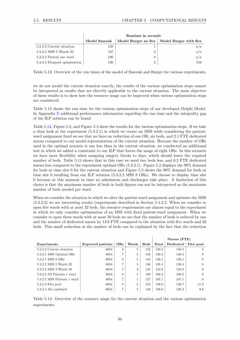
5.5. RESULTS CHAPTER 5. COMPUTATIONAL RESULTS

Runtime in secondsModel Smeenk Model Burger no flex Model Burger with flex

5.2.2.2 Current situation 120 1 n/a5.3.3.2 MSS 5 Wards 32 137 2 n/a5.3.3.2 Patient one ward 586 4 n/a5.3.3.4 Flexpool optimisation 136 2 516

Table 5.13: Overview of the run times of the model of Smeenk and Burger for various experiments.

we do not model the current situation exactly, the results of the various optimisation steps cannotbe interpreted as results that are directly applicable to the current situation. The main objectiveof these results is to show how the resource usage can be improved when various optimisation stepsare considered.

Table 5.13 shows the run time for the various optimisation steps of our developed Delphi Model.In Appendix E additional performance information regarding the run time and the integrality gapof the ILP solution can be found.

Table 5.14, Figure 5.2, and Figure 5.3 show the results for the various optimisation steps. If we takea close look at the experiment (5.3.2.1) in which we create an MSS while considering the patient-ward assignment fixed we see that we have an reduction of one OR, six beds, and 2.1 FTE dedicatednurses compared to our model representation of the current situation. Because the number of ORsused in the optimal scenario is one less than in the current situation, we conducted an additionaltest in which we added a constraint to our ILP that forces the usage of eight ORs. In this scenariowe have more flexibility when assigning surgery blocks to days, which should lower the requirednumber of beds. Table 5.14 shows that in this case we need two beds less, and 0.2 FTE dedicatednurses less compared to the experiment optimal ORs (5.3.2.1). Figure 5.2 displays the 90% demandfor beds at time slot 0 for the current situation and Figure 5.3 shows the 90% demand for beds attime slot 0 resulting from our ILP solution (5.3.2.2 MSS 8 ORs). We choose to display time slot0 because at this moment in time no admissions and discharges take place. A limitation of thischoice is that the maximum number of beds in both figures can not be interpreted as the maximumnumber of beds needed per ward.

When we consider the situation in which we alter the patient-ward assignment and optimise the MSS(5.3.2.2) we see interesting results (experiments described in Section 5.4.2.2. When we consider toopen five wards with at most 32 beds, the resource requirements are almost equal to the experimentin which we only consider optimisation of an MSS with fixed patient-ward assignment. When weconsider to open three wards with at most 50 beds we see that the number of beds is reduced by oneand the number of dedicated nurses by 13.6 FTE compared to the situation with five wards and 32beds. This small reduction in the number of beds can be explained by the fact that the reduction

Nurses (FTE)Experiments Expected patients ORs Wards Beds Total Dedicated Flex pool5.2.2.2 Current situation 6054 8 5 152 140.4 140.4 05.3.2.1 MSS Optimal ORs 6054 7 5 146 138.3 138.3 05.3.2.1 MSS 8 ORs 6054 8 5 144 138.1 138.1 05.3.2.2 MSS 5 Wards 32 6054 7 5 146 138.4 138.4 05.3.2.2 MSS 3 Wards 50 6054 7 3 145 124.8 124.8 05.3.2.2 All Patients 1 ward 6054 8 1 130 108.3 108.3 05.3.2.2 MSS Patients 1 ward 6054 7 1 127 107.1 107.1 05.3.2.3 Flex pool 6054 8 5 152 138.0 126.7 11.35.3.2.4 All combined 6054 7 5 146 136.0 126.2 9.8

Table 5.14: Overview of the resource usage for the current situation and the various optimisationexperiments

50

5.5. RESULTS CHAPTER 5. COMPUTATIONAL RESULTS

in variance in demand for beds for this patient-ward combination is limited. The high reductionin FTE dedicated nurses can be explained by the fact that nurses can be better aligned with thenumber of patients when the patient-to-nurse ratio is high. For example, when the patient-to-nurseratio is eight the optimal number of beds per ward is a multiple of eight. When we consider morepatients per ward we have more efficient usage of dedicated nurses. Table 5.15 displays the resultingpatient-ward assignment for both experiments. When we compare the results for five wards to thecurrent situation we see that the specialties MZK, ORT, CHP and TRA are changed from location.When we allocate all patient types to the same ward, without optimisation of the MSS, we seethat we require 130 beds and 108.3 FTE dedicated nurses. This large reduction in the number ofbeds can be solely accounted for by reduction of variance in demand for beds, while the numberof nurses is partly reduced by better alignment of beds with the patient-to-nurse ratios, and partlyby the reduction in variance in demand. When we compare this result to the experiment in whichwe open three wards, we do not see this reduction in the latter. This can be explained by the factthat the total number of patient types assigned to a ward is too small, or not optimally chosen, totake benefits of variance reduction in demand for beds.

Experiment Ward 0 Ward 1 Ward 2 Ward 3 Ward 4Current URO,VAA CHI,CHIss CHI,CHIss, MZK TRA ORT, CHP5.3.3.3 MSS 5 Wards 32 URO, VAA MZK, ORT CHI, CHIss CHP, TRA CHI, CHIss5.3.3.3 MSS 3 Wards 50 CHP, ORT, VAA MZK, TRA, CHI, CHIss CHI, CHIss

Table 5.15: Overview of the resulting patient-ward assignment from the ILP solution for two opti-misation experiments (5.3.2.2)

The last optimisation stand-alone step considers the use of flex pools (experiment described in Sec-tion 5.4.2.3). When we determine the optimal flex pool-ward combination for the current situationwe can reduce the number of FTEs needed by 2.41. Table 5.16 shows the optimal flex pool-wardcombination for the current situation with flex pools. From the results in Appendix E.5 we see thatthere are large differences in reduction of FTE when we consider all flex pool-ward combinations.The reduction in nurses ranges from 0.1 to 1.8 FTE.

When we consider all various optimisation steps combined we need one OR, six beds, and 4.4 FTEdedicated nurses less than in the current situation (experiment described in Section 5.4.2.4).

Figure 5.2: 90% demand for beds for ward G7 Zuid at time slot 0 for the current situation

Figure 5.3: 90% demand for beds for ward G7 Zuid at time slot 0 resulting from our ILP

51

5.5. RESULTS CHAPTER 5. COMPUTATIONAL RESULTS

Ward Flexpool Nurses (FTE) in flex pool Dedicated nurses (FTE) Realised α Realised β

G6 Zuid 1 3.4 31.5 0.99 0.87G7 Zuid 2 2.2 24.1 0.99 0.90G7 Noord 1 3.4 18.5 0.97 0.94G5 Noord - - 28.5 0.99 0.94G6 Noord 2 2.2 29.8 0.99 0.96

Table 5.16: Best flex pool combination for each ward in the current situation with flex pools andtheir realised service levels (5.3.2.4)

5.5.2 Scenarios

Table 5.17 presents the outcomes of the experiments regarding the two scenarios in which we alterthe input distribution. We first discuss the results of the scenario considering the LOS of patients.Next, we discuss the result of alterations in the number of acute patients.

Nurses (FTE)Experiments Expected patients ORs Wards Beds Total Dedicated Flex pool5.2.2.2 Current situation 6054 8 5 152 140.4 140.4 0.05.3.2.2 MSS 5 Wards 32 6054 7 5 146 138.4 138.4 0.05.3.2.4 All combined 6054 7 5 146 136.0 126.2 9.85.3.4.1 LOS+1 current situation 6054 8 5 174 160.3 160.3 0.05.3.4.1 LOS+1 MSS 5 Wards 6054 7 5 169 155.9 155.9 0.05.3.4.1 LOS+1 All combined 6054 7 5 169 153.9 143.4 10.55.3.4.1 LOS-1 current situation 6054 8 5 138 126.5 126.5 0.05.3.4.1 LOS-1 MSS 5 Wards 6054 7 5 132 126.1 126.1 0.05.3.4.1 LOS-1 All combined 6054 7 5 132 124.0 115.4 8.65.3.4.2 Acute-25% current situation 5222 8 5 135 125.1 125.1 0.05.3.4.2 Acute-25% MSS 5 Wards 5222 7 5 127 122.0 122.0 0.005.3.4.2 Acute-25% All combined 5222 7 5 127 119.6 112.9 6.85.3.4.2 Acute+25% current situation 6522 8 5 162 148.8 148.8 0.05.3.4.2 Acute+25% MSS 5 Wards 6522 7 5 155 145.5 145.5 0.05.3.4.2 Acute+25% All combined 6522 7 5 155 142.8 135.3 7.5

Table 5.17: Overview of the results for the two scenarios on the current situation and the optimi-sation situation

When we increase the LOS of patients the resource needs in the inpatient care chain increase. Whenwe compare scenario LOS+1 MSS 5 Wards to scenario LOS+1 current situation we need five bedsand 4.4 FTE dedicated nurses less. If we compare these reductions to the same experiments inwhich the LOS is normal, we see that the reduction of beds is reduced by one and the total numberof FTE dedicated nurses is increased by 2.1. When we look at the differences between the sametwo scenarios for a decrease in LOS we see that we need six beds and 0.4 FTE dedicated nursesless. If we again compare these reductions to the experiments in which the LOS is normal, we seethat the reduction in beds is the same but the reduction in nurses is almost disappeared.This canbe explained by the fact that

When we compare the benefits of having a flex pool (All combined) to the optimisation scenariowithout a flex pool (MSS 5 Wards 32) we see that the benefits of having a flex pool of nurses isapproximately 2 FTE for both an increase and a decrease in LOS.

Table 5.17 shows that we need 17 beds and 25.3 FTE dedicated nurses less when we reduce thenumber of acute patients by 25% and compare this "new" current situation to the actual currentsituation. When we look at the differences between scenario MSS 5 Wards 32 and scenario currentsituation for both a reduction in acute patients and an increase in acute patients compared to thedifferences in the normal situation we see that our proposed solution approach for both provideshigher result. If we look at the benefits of having a flex pool we notice a difference of 2.4 FTE

52

5.5. RESULTS CHAPTER 5. COMPUTATIONAL RESULTS

dedicated nurses for a decrease of acute patients and 2.7 FTE dedicated nurses for an increase inacute patients.

5.5.3 Sensitivity analysis

In Table 5.18 we present the results of the experiments in which we vary several parameters. Wefirst discuss the outcomes of adaptations of the weighing factors. Next, we explain the outcomesrelated to changing the service levels. We end this section with a discussion of the results regardingan alternative patient-to-nurse ratio.

Nurses (FTE)Experiments Expected patients ORs Wards Beds Total Dedicated Flex pool5.3.2.2 MSS 5 Wards 32 6054 7 5 146 138.4 138.4 0.05.3.5.1 ILP Exp 1. 6054 8 5 146 139.5 139.5 0.05.3.5.1 ILP Exp 2. 6054 8 5 146 137.1 137.1 0.05.2.2.2 Current situation 6054 8 5 152 140.4 140.4 0.05.3.2.4 Flex pool optimisation 6054 8 5 152 138.0 126.7 11.35.3.5.2 Serv lvls (0.80,0.80,0.66) no flex 6054 8 5 152 132.3 132.3 0.05.3.5.2 Serv lvls (0.80,0.80,0.66) flex 6054 8 5 152 132.3 132.3 0.05.3.5.2 Serv lvls (0.80,0.70,0.66) no flex 6054 8 5 152 123.7 123.7 0.05.3.5.2 Serv lvls (0.80,0.70,0.66) flex 6054 8 5 152 122.8 114.5 8.35.3.5.2 Serv lvls (0.80,0.70,0.50) no flex 6054 8 5 152 123.7 123.7 0.05.3.5.2 Serv lvls (0.80,0.70,0.50) flex 6054 8 5 152 120.3 114.5 5.85.3.5.2 Patient-nurse ratio no flex 6054 8 5 152 136.5 136.5 0.05.3.5.2 Patient-nurse ratio flex 6054 8 5 152 134.2 126.3 7.9

Table 5.18: Overview of the results for the sensitivity experiments

When we adapt the weighing factors of the ILP (experiments described in Section 5.4.4.1) we seeno difference in number of beds needed between the three experiments. However, a difference intotal number of dedicated nurses can be noticed. The first experiment (5.3.5.1 ILP Exp 1) requires1.1 FTE dedicated nurses more and the second experiment (5.3.5.1 ILP Exp 2) requires 1.3 FTEof dedicated nurses less compared to our initial ILP solution (5.3.2.2 MSS 5 Wards 32). Table5.19 shows the resulting patient-ward assignment for both experiments. When we compare thisassignment to the initial experiment from Section 5.4.2.2 we see some interesting results. In allexperiments patient types URO and VAA are allocated to the same ward, and the same holds forpatient types CHI and CHIss. The patient types MZK, ORT, TRA and CHP are assigned in adifferent manner in each experiment. The patient-ward assignment differs between all scenariosbecause due to these changing weights CPLEX chooses an alternative solution. We can explain thedifference in total number of nurses for both experiments by differences in alignment of the demandfor beds to the patient-to-nurse ratio.

Experiment Ward 0 Ward 1 Ward 2 Ward 3 Ward 45.3.3.3 MSS 5 Wards 32 URO, VAA MZK, ORT CHI, CHIss CHP, TRA CHI, CHIss5.3.5.1 Exp 1 CHI, CHIss TRA CHI, CHIss MZK, URO , VAA CHP, ORT5.3.5.1 Exp 2 CHI, CHIss ORT URO, VAA CHI, CHIss CHP, MZK, TRA

Table 5.19: Overview of the resulting patient-ward assignment from the ILP solution for experimentswith different weight factors

When we alter the nurse service level requirements (experiments described in Section 5.4.4.2) wesee that lowering the overall service level and minimum service level both have a positive effect onthe total number of nurses needed. When we set the overall service level equal to the minimumservice level the benefits of having a flex pool are reduced to zero FTE reduction (5.3.5.2 Servlvls (0.80,0.80,0.66)). This is to be expected because both service levels are equal and the method

53

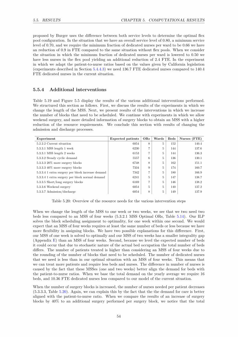
5.5. RESULTS CHAPTER 5. COMPUTATIONAL RESULTS

proposed by Burger uses the difference between both service levels to determine the optimal flexpool configuration. In the situation that we have an overall service level of 0.80, a minimum servicelevel of 0.70, and we require the minimum fraction of dedicated nurses per ward to be 0.66 we havean reduction of 0.9 in FTE compared to the same situation without flex pools. When we considerthe situation in which the minimum fraction of dedicated nurses per ward is lowered to 0.50 wehave less nurses in the flex pool yielding an additional reduction of 2.4 FTE. In the experimentin which we adapt the patient-to-nurse ratios based on the values given by California legislation(experiments described in Section 5.4.4.3) we need 136.7 FTE dedicated nurses compared to 140.4FTE dedicated nurses in the current situation.

5.5.4 Additional interventions

Table 5.19 and Figure 5.5 display the results of the various additional interventions performed.We structured this section as follows. First, we discuss the results of the experiments in which wechange the length of the MSS. Next, we present results of the interventions in which we increasethe number of blocks that need to be scheduled. We continue with experiments in which we allowweekend surgery, and more detailed information of surgery blocks to obtain an MSS with a higherreduction of the resource requirements. We conclude this section with results of changing theadmission and discharge processes.

Experiment Expected patients ORs Wards Beds Nurses (FTE)5.2.2.2 Current situation 6054 8 5 152 140.45.3.3.1 MSS length 1 week 6230 7 5 144 137.65.3.3.1 MSS length 2 weeks 6153 7 5 144 136.35.3.3.2 Steady cyclic demand 5557 6 5 136 130.15.3.3.3 20% more surgery blocks 6748 8 5 162 151.15.3.3.3 40% more surgery blocks 7334 9 5 174 160.75.3.3.4 1 extra surgery per block increase demand 7342 7 5 180 166.95.3.3.4 1 extra surgery per block normal demand 6241 5 5 147 138.75.3.3.5 Short/long surgery blocks 6169 7 5 146 138.25.3.3.6 Weekend surgery 6054 5 5 140 137.25.3.3.7 Admission/discharge 6054 8 5 149 137.9

Table 5.20: Overview of the resource needs for the various intervention steps

When we change the length of the MSS to one week or two weeks, we see that we two need twobeds less compared to an MSS of four weeks (5.3.2.1 MSS Optimal ORs, Table 5.14). Our ILPsolves the block scheduling assignment to optimality, for one week within one second. We wouldexpect that an MSS of four weeks requires at least the same number of beds or less because we havemore flexibility in assigning blocks. We have two possible explanations for this difference. First,our MSS of one week is solved to optimally and our MSS of two weeks has a smaller integrality gap(Appendix E) than an MSS of four weeks. Second, because we level the expected number of bedsit could occur that due to stochastic nature of the actual bed occupation the total number of bedsdiffers. The number of patients treated is higher than considering an MSS of four weeks due tothe rounding of the number of blocks that need to be scheduled. The number of dedicated nursesthat we need is less than in our optimal situation with an MSS of four weeks. This means thatwe can treat more patients and require less beds and nurses. The difference in number of nurses iscaused by the fact that these MSSes (one and two weeks) better align the demand for beds withthe patient-to-nurse ratios. When we base the total demand on the yearly average we require 16beds, and 10.36 FTE dedicated nurses less compared to our model of the current situation.

When the number of surgery blocks is increased, the number of nurses needed per patient decreases(5.3.3.3, Table 5.20). Again, we can explain this by the fact that the the demand for care is betteraligned with the patient-to-nurse ratio. When we compare the results of an increase of surgeryblocks by 40% to an additional surgery performed per surgery block, we notice that the total

54

5.5. RESULTS CHAPTER 5. COMPUTATIONAL RESULTS

expected number of patients treated is equal, while the required number of resources is lower forthe situation in which we have more surgery blocks. We can explain this as follows. When wehave more surgery blocks to schedule with fewer surgeries we are more capable to level the requirednumber of beds and thereby reduce the variance in demand for care.

When we consider the output of the scenarios with long surgeries and short surgeries (5.3.3.5, Table5.20) we would expect that the demand for beds and nurses is lower compared to the situationin which we consider only one generic surgery block per patient type. However, the results arecomparable and not lower. This difference can be explained by the increased number of surgeriesthat are scheduled. Another reason may be that the differentiation between surgery blocks is notdetailed enough. The scenario in which we consider weekend surgery (5.3.3.6, Table 5.20) reducedthe number of ORs used by three and the number of beds by twelve compared to the currentsituation. The total number of dedicated nurses needed is only slightly affected. Figure 5.4 showsthe 90% demand for beds when we allow surgery during weekends. We can see that our ILP solutionimproves the leveling of number of occupied beds compared to the 90% demand for beds in Figure5.2 and Figure 5.3.

When we adjust the admission and discharge process of elective patients (5.3.3.7, Table 5.20), we canconclude that we need three beds and 2.6 FTE dedicated nurses less than in the current situation.

Figure 5.4: 90% demand for beds for ward G7 Zuid at time slot 0 for the scenario in which we allowweekend surgery

5.5.5 Comparison of all interventions

In this section we determine which interventions from Section 5.4.2 and the additional interventionsfrom Section 5.4.5 have the most potential to improve the resource utilisation compared to ourmodel representation of the current situation (Section 5.4.1). We determine the efficiency of anintervention by calculating the efficient frontier, in which we divide output by input. We choose tocompare all outcomes of the interventions based on the resources nurses and beds because these aredirectly comparable to our model of the current situation. We do not choose to base the outcomeson total costs because the obtained cost figures are relatively rough estimates. We do not considerthe total number of ORs required because this is in practice also influenced by surgery requestsfor other divisions. Figure 5.5 shows the efficient frontier for all interventions. The interventionsin which we allocate all patients to the same ward are excluded because these interventions are ofan exploratory nature. On the horizontal axis we show the number of expected patients per year(output) divided by the total number of beds needed (input). On the vertical axis we show theexpected number of patients per year (output) divided by the total FTE of nurses needed (input).The dotted line is the efficient frontier, which denotes the interventions that are 100% efficient. Weuse the term 100% efficient because it is not possible to improve on one indicator without worseningthe other.

Figure 5.5 shows that our model of the current situation (located in the figure on the bottom left)scores worse compared to almost all interventions. The only intervention that scores lower on thenumber of nurses per patient is the scenario in which we consider a steady cyclic demand and less

55

5.5. RESULTS CHAPTER 5. COMPUTATIONAL RESULTS

Figure 5.5: Overview of the efficient frontier for the various interventions and optimisation experi-ments

patients are treated. Figure 5.5 shows that there are three most promising interventions. Mostbeneficial for efficient alignment of nurses to demand for care is to consider three wards with amaximum bed size of 50. Due to the larger ward sizes and better alignment with the patient-to-nurse ratio less nurses can treat more patients. Most beneficial for reducing the number of bedsis considering an MSS with a length of 1 week. The reason that this intervention performs betterthan for example an MSS of two weeks is twofold. First, when we consider an MSS with a length of1 week we have a lower complexity of scheduling of surgery blocks. Because we manually stop ourILP after 30 minutes it could occur that our 1 week MSS solution is solved to optimality but our2 weeks MSS solution is not yet solved to optimality. Second, we had to round the total numberof surgery blocks that need to be scheduled, which also explains a difference. When we increasethe number of patients per surgery block while considering the same amount of surgery blocks, wenotice that this intervention gives the best results in both directions. From this figure, we alsoconclude that all interventions in which the number of patient is increased are beneficial for thenumber of nurses in FTE and beds per patient required.

Table 5.21 shows the improvement potential for the three most promising interventions comparedto our model of the current situation. When we consider 3 wards with 50 beds we can treat 11.1%more patients with the same number of FTE nurses or decrease the total FTE of nurses by 11.1%while treating the same number of patients. We conducted an additional experiment that consistsof a combination of the interventions MSS length 1 week and MSS 3 wards 50 beds. Table 5.21shows that this scenario even performs better, yielding a reduction of 12.0% in expected patientsper nurse in FTE and a reduction of 11.8% in expected patients per bed.

56

5.6. CONCLUSIONS CHAPTER 5. COMPUTATIONAL RESULTS

Improvement potential %Experiment Patients/FTE nurse/year Patients/bed/year Patients/nurse/year Patients/bed/yearCurrent situation 43.1 39.8 - -5.3.3.1 MSS length 1 week 45.3 43.3 4.8% 8.0%5.3.2.3 MSS 3 Wards 50 48.5 41.8 11.1% 4.7%5.3.3.4. 1 extra surgery per block a 46.3 42.9 6.9% 7.2%5.5.5 MSS length 1 week, 3 wards 50 49.0 45.1 12.0% 11.8%

Table 5.21: Improvement potential of the best interventions compared to our model of the currentsituation

5.6 Conclusions

In this chapter we conducted several experiments to show the performance of our solution approachand to determine profitable interventions to improve the resource usage in the inpatient care chain.

Based on our approach we conclude that our ILP to create an MSS, as expected, minimises themaximum number of beds required per ward and thereby levels the workload. When we considerthe ILP to make the patient-ward assignment decision we see that reducing the number of wardsdoes not necessarily require a lower total amount of beds. However, a reduction of wards combinedwith an increase in total number of patients per ward is beneficial for the total number of nursesrequired, due to better alignment of demand care with the patient-to-nurse ratio. A shortcoming ofour ILP solution approach is that, due to the large amount of variables, it is not possible with ourset-up to take the nursing requirements into account when creating the MSS, and deciding uponthe patient-ward assignment. Therefore, we only focus on minimisation of the maximum numberof beds. When considering the use of flex pools, we conclude in most experiments a reduction oftwo FTE is achieved. Furthermore, we have noticed that the block scheduling decision and the flexpool-ward assignment influences the added value of a flex pool between two wards in terms of totalFTE nurse reduction (experiment 5.4.2.3).

Based on the scenario analysis, we conclude that our solution approach outperforms our model ofthe current situation for changes in the LOS of patients or in the total number of acute patients.When the LOS is changed we see that the difference in resource needs between our solution approachand our model of the current situation is reduced when the LOS is decreased, and increased whenthe LOS of patients is increased. When the number of acute patients changes the difference inresource needs between our model of the current situation and our optimisation methods remainsalmost the same.

After conducting a sensitivity analysis of the weighing factors we conclude that the resource re-quirements of our ILP hardly changes, but that these weights do influence the patient-to-wardassignment and the block scheduling decision. Reducing the service level requirements of nurses isbeneficial for reducing the total number of nurses needed, but could endanger the quality of care.

From the additional interventions conducted we conclude that a higher amount of surgery blocksin combination with more detailed information about these surgery blocks yields opportunities toincrease the utilisation of beds and nurses. When considering an alternative discharge and admissionprocedure additional savings can be achieved in a rather easy manner. The reductions that we obtainin each intervention have the same level of quality of care as in our model representation of thecurrent situation, due to the predefined target service levels.

When we compare the improvement potential of our model of the current situation to the interven-tions conducted, we see that three wards with at most 50 beds reduces the total number of FTEnurses required by 11.1%. When we want to reduce the number of beds, an MSS with a length ofone week is most benefical, yielding a reduction of 8.0% in beds. When we consider an interventionthat consists of three wards with at most 50 beds and an MSS length of one week, we require 12.0%less nurses and 11.8% less beds or we can increase the number of patients by these percentages,while keeping the same number of FTE and beds as in our model of the current situation.

57

Chapter 6

Conclusions & recommendations

In this chapter we reflect on our approach to reach our research objective. Section 6.1 containsthe conclusions we draw from this research. In Section 6.2 we discuss our proposed model andthe applicability of the results. Section 6.3 states the recommendations we give to the AMC toimprove utilisation of resources in the inpatient care chain. Section 6.4 concludes with suggestionsfor further research.

6.1 Conclusions

In this research we provide insight in the complex relations between resource capacity planningdecisions in the OR department and the clinical nursing wards to support decision making byhealth care managers and to make efficient use of resources. The objective of this research is: Todevelop a method which determines the best combination of patient case mix, OR capacity, careunit and nurse staffing decisions in such way that total cost margins are maximised while satisfyingproduction agreements and resource, capacity, and quality constraints.

To reach our research objective we conducted a literature study in Chapter 3 to find methodsand models related to resource capacity planning decisions. In Chapter 4 we defined our researchobjective as a mathematical optimisation problem, and we proposed a decomposition approach tosolve this problem. Our approach consists of the following six steps:

1. Set the desired patient case mix and the length of the MSS.

2. Solve an ILP to create a master surgical schedule and assign elective and acute patient typesto wards, while minimising the number of ORs, wards, and the expected number of nursesand beds required.

3. Evaluate the access time service level of the created block schedule with the model of Kortbeeket al. [19].

4. Determine the number of beds required per ward while satisfying target rejection and mis-placement rates with the model of Smeenk et al. [29].

5. Iteratively use the model of Burger et al. (Step 6) to determine the best flex pool-wardcombination.

6. Determine the optimal number of dedicated nurses per ward and the total number of nursesin a flex pool given various target service levels with the model of Burger et al. [9].

59

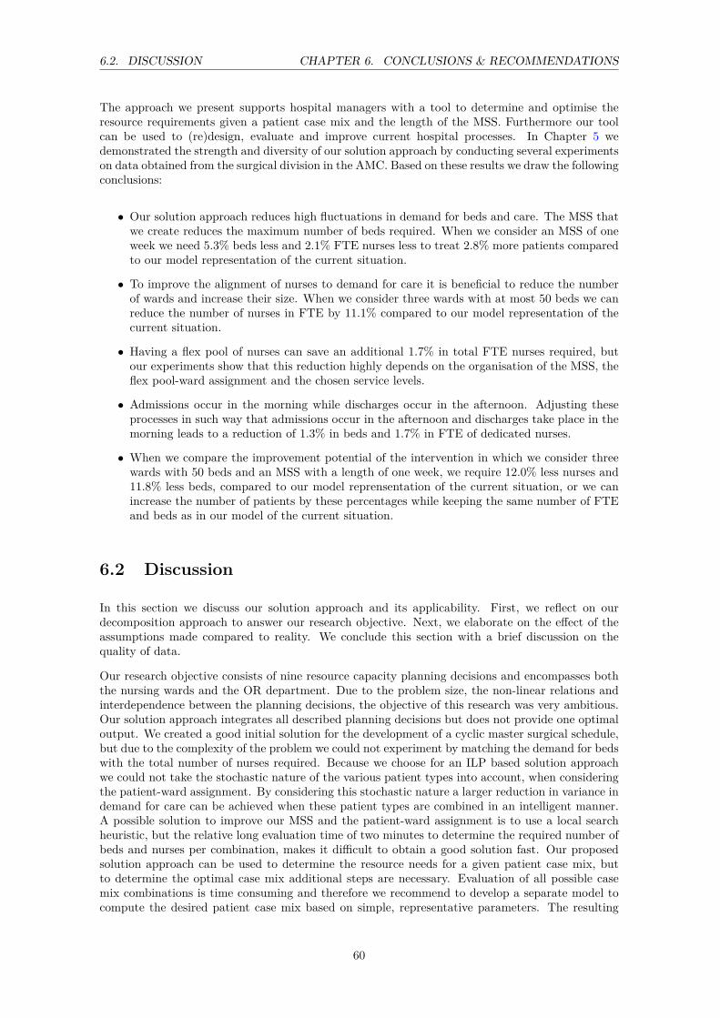
6.2. DISCUSSION CHAPTER 6. CONCLUSIONS & RECOMMENDATIONS

The approach we present supports hospital managers with a tool to determine and optimise theresource requirements given a patient case mix and the length of the MSS. Furthermore our toolcan be used to (re)design, evaluate and improve current hospital processes. In Chapter 5 wedemonstrated the strength and diversity of our solution approach by conducting several experimentson data obtained from the surgical division in the AMC. Based on these results we draw the followingconclusions:

• Our solution approach reduces high fluctuations in demand for beds and care. The MSS thatwe create reduces the maximum number of beds required. When we consider an MSS of oneweek we need 5.3% beds less and 2.1% FTE nurses less to treat 2.8% more patients comparedto our model representation of the current situation.

• To improve the alignment of nurses to demand for care it is beneficial to reduce the numberof wards and increase their size. When we consider three wards with at most 50 beds we canreduce the number of nurses in FTE by 11.1% compared to our model representation of thecurrent situation.

• Having a flex pool of nurses can save an additional 1.7% in total FTE nurses required, butour experiments show that this reduction highly depends on the organisation of the MSS, theflex pool-ward assignment and the chosen service levels.

• Admissions occur in the morning while discharges occur in the afternoon. Adjusting theseprocesses in such way that admissions occur in the afternoon and discharges take place in themorning leads to a reduction of 1.3% in beds and 1.7% in FTE of dedicated nurses.

• When we compare the improvement potential of the intervention in which we consider threewards with 50 beds and an MSS with a length of one week, we require 12.0% less nurses and11.8% less beds, compared to our model reprensentation of the current situation, or we canincrease the number of patients by these percentages while keeping the same number of FTEand beds as in our model of the current situation.

6.2 Discussion

In this section we discuss our solution approach and its applicability. First, we reflect on ourdecomposition approach to answer our research objective. Next, we elaborate on the effect of theassumptions made compared to reality. We conclude this section with a brief discussion on thequality of data.

Our research objective consists of nine resource capacity planning decisions and encompasses boththe nursing wards and the OR department. Due to the problem size, the non-linear relations andinterdependence between the planning decisions, the objective of this research was very ambitious.Our solution approach integrates all described planning decisions but does not provide one optimaloutput. We created a good initial solution for the development of a cyclic master surgical schedule,but due to the complexity of the problem we could not experiment by matching the demand for bedswith the total number of nurses required. Because we choose for an ILP based solution approachwe could not take the stochastic nature of the various patient types into account, when consideringthe patient-ward assignment. By considering this stochastic nature a larger reduction in variance indemand for care can be achieved when these patient types are combined in an intelligent manner.A possible solution to improve our MSS and the patient-ward assignment is to use a local searchheuristic, but the relative long evaluation time of two minutes to determine the required number ofbeds and nurses per combination, makes it difficult to obtain a good solution fast. Our proposedsolution approach can be used to determine the resource needs for a given patient case mix, butto determine the optimal case mix additional steps are necessary. Evaluation of all possible casemix combinations is time consuming and therefore we recommend to develop a separate model tocompute the desired patient case mix based on simple, representative parameters. The resulting

60

6.3. RECOMMENDATIONS CHAPTER 6. CONCLUSIONS & RECOMMENDATIONS

case mix can then be imported in our developed model to obtain a more detailed view of the actualresource needs.

To reduce modelling complexity we made several assumptions. These assumptions are necessary tocapture the real situation in a model. In the real situation a lot of variation in the daily processesof patients is present. For example, some patients undergo more than one surgery or visit multiplewards during their hospital stay. It is undesirable and not possible to capture all these variations inan analytical model. Therefore, our modelling approach is not a tool that mimics the real situationin exact detail, but a tool that can be used to study the effect of various resource capacity planninginterventions on the resource requirements.

Our solution approach consists of an exact model that requires reliable historic data. The qualityof the data available in the AMC was sufficient to demonstrate our solution approach and to seethe influence of various interventions on the total resource requirements. However, more reliableresults can be achieved when the quality of data is improved.

6.3 Recommendations

In Chapter 2 we identified possible causes that yield a low bed occupation, a high number of nursesstaffed and high variance in number of patients that undergo surgery within a surgery block. Basedon the results of the experiments we conducted, we give the following recommendations to the AMCto make more efficient use of resources in the inpatient care chain:

• Reduce number of wards and increase their size: Reduce the total number of wardsby assigning multiple patient types to the same ward. When we consider less wards withmore beds we reduce the variance in demand for beds and care that results from the MSS.Thereby we increase the bed occupancy and require smaller total numbers of beds and FTEdedicated nurses. When we consider an intervention in which we consider three wards witha maximum of 50 beds, we save 11.1% FTE compared to our model of the current situation.Another advantage of reducing the number of wards is the possibility to save additional costsby integration of several overhead functions. For example, the secretary staff of both wardscan be combined and less square meters are required. When considering a combination ofmultiple patient types into the same ward it is important to research whether nurses requireadditional training. We recommend that the size of a ward is not increased too much, whichcould result in patients’ dissatisfaction, safety concerns and managing difficulties.

• Opportunities MSS: The solution approach we present consists of a method to create acyclic master surgical schedule while lowering the maximum number of beds required. Weshow that we can reduce the total number of beds required by 5.3% compared to the modelof the current situation. Another advantage of a cyclic MSS is that it provides the possiblityto predict the demand for beds and care, and thereby determine the number of nurses tobe staffed per shift in advance. Additional reductions can be achieved when more detailedinformation on the number of patients in a surgery block is known or when less acute patientsare considered. We recommend to perform additional research into the development of anMSS that focuses on better alignment in the demand for beds and care in the nursing wards.

• Flex pool of nurses: A flex pool of nurses reduces the total number of nurses required,while maintaining predefined service levels. The total reduction in FTE is rather limited inour experiments due to the MSS and the chosen service levels, so considering a flex pool ofnurses mainly depends on the additional costs required, such as extra training to treat morethan one patient type. If these additional costs are low compared to the reduction in FTE,we would recommend to use a flex pool of nurses.

• Perform additional experiments with misplacements: In our experimental design wedid not conduct experiments regarding the possibility of misplacing patients between twowards, because the realised rejection and misplacement rates of the model of Smeenk et al.

61

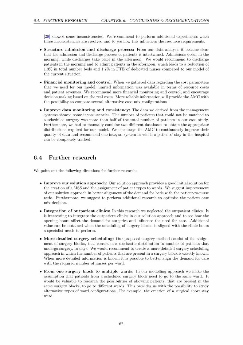
6.4. FURTHER RESEARCH CHAPTER 6. CONCLUSIONS & RECOMMENDATIONS

[29] showed some inconsistencies. We recommend to perform additional experiments whenthese inconsistencies are resolved and to see how this influences the resource requirements.

• Structure admission and discharge process: From our data analysis it became clearthat the admission and discharge process of patients is intertwined. Admissions occur in themorning, while discharges take place in the afternoon. We would recommend to dischargepatients in the morning and to admit patients in the afternoon, which leads to a reduction of1.3% in total number beds and 1.7% in FTE of dedicated nurses compared to our model ofthe current situation.

• Financial monitoring and control: When we gathered data regarding the cost parametersthat we need for our model, limited information was available in terms of resource costsand patient revenues. We recommend more financial monitoring and control, and encouragedecision making based on the real costs. More reliable information will provide the AMC withthe possibility to compare several alternative case mix configurations.

• Improve data monitoring and consistency: The data we derived from the managementsystems showed some inconsistencies. The number of patients that could not be matched toa scheduled surgery was more than half of the total number of patients in our case study.Furthermore, we had to manually combine two different databases to obtain the appropriatedistributions required for our model. We encourage the AMC to continuously improve theirquality of data and recommend one integral system in which a patients’ stay in the hospitalcan be completely tracked.

6.4 Further research

We point out the following directions for further research:

• Improve our solution approach: Our solution approach provides a good initial solution forthe creation of a MSS and the assignment of patient types to wards. We suggest improvementof our solution approach in better alignment of the demand for beds with the patient-to-nurseratio. Furthermore, we suggest to perform additional research to optimise the patient casemix decision.

• Integration of outpatient clinics: In this research we neglected the outpatient clinics. Itis interesting to integrate the outpatient clinics in our solution approach and to see how theopening hours affect the demand for surgeries and influence the need for care. Additionalvalue can be obtained when the scheduling of surgery blocks is aligned with the clinic hoursa specialist needs to perform.

• More detailed surgery scheduling: Our proposed surgery method consist of the assign-ment of surgery blocks, that consist of a stochastic distribution in number of patients thatundergo surgery, to days. We would recommend to create a more detailed surgery schedulingapproach in which the number of patients that are present in a surgery block is exactly known.When more detailed information is known it is possible to better align the demand for carewith the required number of nurses per ward.

• From one surgery block to multiple wards: In our modelling approach we make theassumption that patients from a scheduled surgery block need to go to the same ward. Itwould be valuable to research the possibilities of allowing patients, that are present in thesame surgery blocks, to go to different wards. This provides us with the possibility to studyalternative types of ward configurations. For example, the creation of a surgical short stayward.

62

Bibliography

[1] Groot personeelstekort zorg verwacht in 2025. http://www.zorgwelzijn.nl/web/Actueel/Nieuws/Groot-personeelstekort-zorg-verwacht-in-2025.htm. 2

[2] Kwaliteit en proces innovatie. http://intranet.amc.uva.nl/?pid=8721. 1

[3] I. Adan, J. Bekkers, N. Dellaert, J. Jeunet, and J. Vissers. Improving operational effectivenessof tactical master plans for emergency and elective patients under stochastic demand andcapacitated resources. European Journal of Operational Research, 213:290–308, 2011. 23, 34

[4] L.H. Aiken, D.M. Sloane, J.P Cimiotti, S.P. Clarke, L. Flynn, J.A. Seago, J. Spetz, and H.L.Smith. Implications of the california nurse staffing mandate for other states. Health Researchand Educational Trust, 2010. 47

[5] J. Beliën and E. Demeulemeester. Building cyclic master surgery schedules with leveled bedoccupancy. European Journal of Operational Research, 176:1185–1204, 2007. 20, 22

[6] J. Beliën, E. Demeulemeester, and B. Cardoen. A decision support system for cyclic mastersurgery scheduling with multiple objectives. Journal of Scheduling, 12:147–161, 2009. 23

[7] J.M. Bosch. Better utilisation of the or with less beds: A tactical surgery scheduling approachto improve or utilisation and the required number of beds in the wards. Master’s thesis,University of Twente, 2011. 22

[8] A. Braaksma and N. Kortbeek. Adviesreport: Herziening indeling beddenhuis divisie b. AMC.9, 14, 43

[9] C.A.J. Burger. Flexible nurse staffing: Determining staffing levels for nursing wards in theamc. Master’s thesis, University of Twente, 2011. i, ii, 1, 2, 3, 5, 22, 32, 37, 38, 59

[10] E.K. Burke, P. De Causmaecker, G. Vanden Berghe, and H. Van Landeghem. The state of theart of nurse rostering. Journal of Scheduling, 7:441–499, 2004. 22

[11] B. Cardoen, E. Demeulemeester, and J. Beliën. Operating room planning and scheduling: Aliterature review. European Journal of Operational Research, 201:921–932, 2010. 19, 20

[12] Y. Carson and A. Maria. Simulation optimization: Methods and applications. In Proceedingsof the 1997 Winter Simulation Conference, 1997. 19

[13] J.K. Cochran and A. Bharti. Stochastic bed balancing of an obstetrics hospital. Health CareManagement Science, 9:31–45, 2006. 19, 21

[14] D. Cornelisse. Ok-reglement 2011: Operatiecentrum (klinische ok en dagcentrum), divisie h,amc. AMC. 11, 12

[15] F. Guerriero and R. Guido. Operational research in the management of the operating theatre:a survey. Health Care Management Science, 14:89–114, 2011. 2, 20

[16] E.W. Hans, M. Van Houdenhoven, and P.J.H. Hulshof. A framework for health care planningand control. Handbook of Healthcare System Scheduling. International Series in OperationsResearch & Management Science, 168:303–320, 2012. 3, 5

63

BIBLIOGRAPHY BIBLIOGRAPHY

[17] P.J.H. Hulshof, N. Kortbeek, R.J. Boucherie, and E.W. Hans. Taxonomic classification ofplanning decisions in health care: a review of the state of the art in or/ms. Center forHealthcare Operations Improvement and Research, -:–, 2011. i, 1, 5, 19

[18] J.B. Jun, S.H. Jacobson, and J.R. Swisher. Application of disrete-event simulation in healthcare clinics: A survey. Journal of the Operational Research Society, 50:109–123, 1999. 19

[19] N. Kortbeek, E.M. Zonderland, R. J. Boucherie, N. Litvak, and E.W. Hans. Desidesigningcyclic appointment schedules for outpatient clinics with scheduled and unscheduled patientarrivals. Memorandum 1968 December 2011. i, 35, 59

[20] A.M. Law. Simulation modeling and analysis: Fourth edition. McGraw-Hill InternationalEdition, 2007. 39

[21] G. Ma, J. Beliën, E. Demeulemeester, and L. Wang. Solving the strategic case mix problemoptimally by using branch and price algorithms. In Proceedings of the 35th InternationalConference on Operational Research Applied to Health Services, 2009. 20

[22] M. Maiza. Heuristics for solving the bin-packing problem with conflicts. Applied MathematicalSciences, 5:1739 – 1752, 2011. 33

[23] J.H. May, W.E. Spangler, D.P. Strum, and L.G. Vargas. The surgical scheduling problem:Current research and future opportunities. Production and Operations Management, 20:392–405, 2011. 20

[24] M.W. Mullholand, P. Abrahamse, and V. Bahl. Linear programming to optimize performancein a department of surgery. The american college of surgeons, published by Elsevier, 2005. 20

[25] A.E.F Muritiba, M. Lori, E. Malaguti, and P. Toth. Algorithms for the bin packing problemwith conflicts. INFORMS Journal on Computing, 22:401–415, 2010. 33

[26] J. Needleman, P. Buerhaus, V.S. Pankratz, C.L. Leibson, S.R. Stevens, and M. Harris. Nursestaffing and inpatient hospital mortality. New England Journal of Medicine, 364:1037–1045,2011. 2

[27] J.M. Nguyen, P. Six, D. Antonioli, P. Glemain, G. Potel, P. Lombrail, and P. Le Beux. A simplemethod to optimize hospital beds capacity. International Journal of Medical Informatics,74:39–49, 2005. 21

[28] P. Santibáñez, B. Mehmet, and D. Atkins. Surgical block scheduling in a system of hospitals:an application to resource and wait list management in a british columbia health authority.Health Care Management Science, 10:269–282, 2007. 23

[29] H.F. Smeenk. Predicting bed census of nursing ward from hour to hour. Master’s thesis,University of Twente, 2011. i, 1, 2, 3, 5, 12, 21, 22, 36, 37, 59, 62

[30] H.F. Smeenk and C.A.J. Burger. Bed capacity management and nurse scheduling: Processdescription g6. AMC. 9, 10, 12, 14

[31] V.L. Smith-Daniels, S.B. Schweikhart, and D.E Smith-Daniels. Capacity management in healthcare services: Review and future research directions. Decision Sciences, 19:889–919, 1988. 15

[32] A. Testi, E. Tanfani, and G. Torre. A three-phase approach for operating theatre schedules.Health Care Management Science, 10:163–172, 2007. 20

[33] J. M. Van Oostrum, M. Van Houdenhoven, J. L. Hurink, E.W. Hans, G. Wullink, andG. Kazemier. A master surgical scheduling approach for cyclic scheduling in operating roomdepartments. Operation Research Spectrum, 30:355–374, 2008. 21, 22

[34] J.M. Van Oostrum, E. Bredenhoff, and E.W. Hans. Suitability and managerial implications ofa master surgical scheduling approach. Annals of Operations Research, 178:91–104, 2010. 20

64

BIBLIOGRAPHY BIBLIOGRAPHY

[35] P.T. Vanberkel and J.T. Blake. A comprehensive simulation for wait time reduction andcapacity planning applied in general surgery. Health Care Management Science, 10:373–385,2007. 19

[36] P.T. Vanberkel, R.J. Boucherie, E.W. Hans, J.L. Hurink, and N. Litvak. A survey of healthcare models that encompass multiple departments. International journal of health managementand information, 1:37–69, 2010. 9, 19, 22

[37] P.T. Vanberkel, R.J. Boucherie, E.W. Hans, J.L. Hurink, W.A.M. Van Lent, and Van HartenW.H. An exact approach for relating recovering surgical patient workload to the master surgicalschedule. Journal of the Operational Research Society, 62:1851–1860, 2010. 2, 3, 21, 22

[38] S. Villa, M. Barbieri, and F. Lega. Restructuring patient flow logistics around patient careneeds: implications and practicalities from three critical cases. Health Care ManagementScience, 12:155–165, 2009. 21

65

Appendix A

Mathematical optimisationproblem and ILP

This appendix summarises the notation used for the mathematical optimisation problem defined inSection 4.1 and the ILP defined in Section 4.2.2. We define the sets, parameters, distributions anddecision variables for the mathematical optimisation problem in Section A.1. Section A.2 containsthe sets, parameters, distributions and decision variables of the ILP.

A.1 Notation mathematical optimisation problem

Sets

JE Set of elective patient typesJA Set of acute patient typesJ Set of all patient types, JE

⋃JA

R Set of resources in the ORW Set of wards inside the hospitalF Set of flex pools

Parameters

General parameters:D Number of working days in a weekT Number of time slotsT Number of shift typesbigM Some large numberµj,d Average number of appointment request for patient type j on day d,

j ∈ JE , d ∈ 0, . . . , D − 1λj,d,t Poisson arrival rate of patient type j on day d during timeslot t,

j ∈ JA, d ∈ 0, . . . , D − 1, t ∈ 0, . . . , T − 1

67

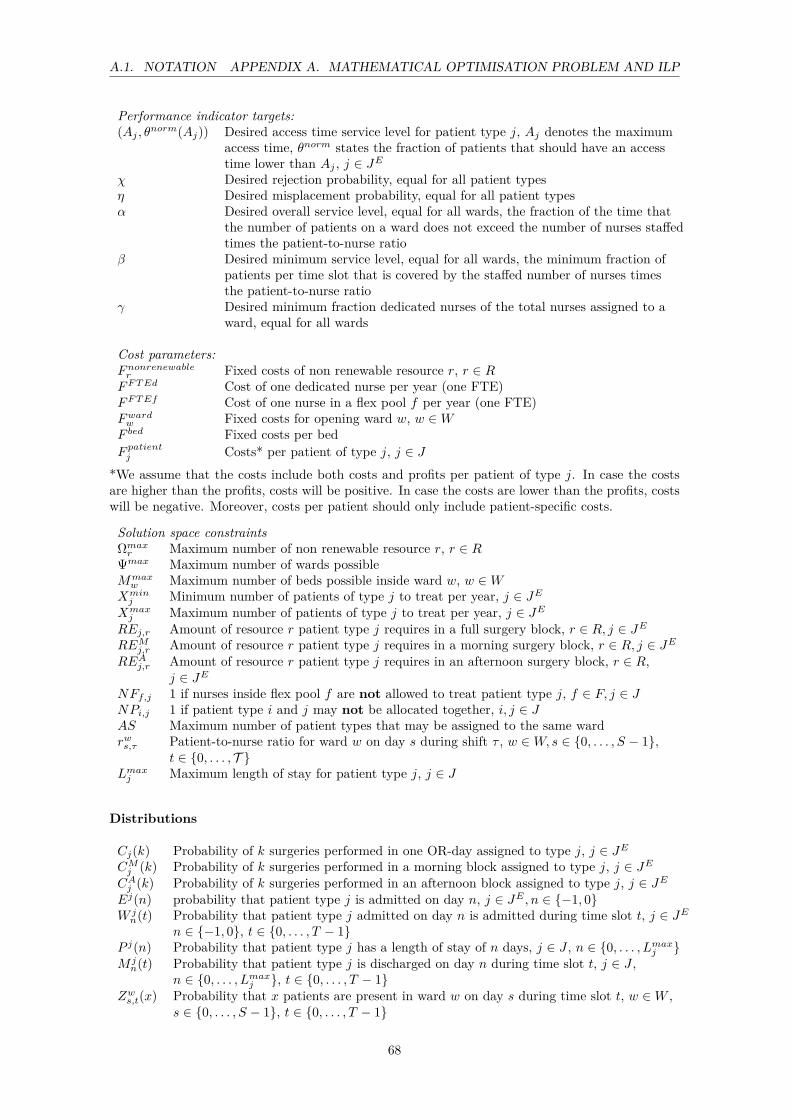
A.1. NOTATION APPENDIX A. MATHEMATICAL OPTIMISATION PROBLEM AND ILP

Performance indicator targets:(Aj , θnorm(Aj)) Desired access time service level for patient type j, Aj denotes the maximum

access time, θnorm states the fraction of patients that should have an accesstime lower than Aj , j ∈ JE

χ Desired rejection probability, equal for all patient typesη Desired misplacement probability, equal for all patient typesα Desired overall service level, equal for all wards, the fraction of the time that

the number of patients on a ward does not exceed the number of nurses staffedtimes the patient-to-nurse ratio

β Desired minimum service level, equal for all wards, the minimum fraction ofpatients per time slot that is covered by the staffed number of nurses timesthe patient-to-nurse ratio

γ Desired minimum fraction dedicated nurses of the total nurses assigned to award, equal for all wards

Cost parameters:Fnonrenewabler Fixed costs of non renewable resource r, r ∈ RFFTEd Cost of one dedicated nurse per year (one FTE)FFTEf Cost of one nurse in a flex pool f per year (one FTE)Fwardw Fixed costs for opening ward w, w ∈WF bed Fixed costs per bedF patientj Costs* per patient of type j, j ∈ J

*We assume that the costs include both costs and profits per patient of type j. In case the costsare higher than the profits, costs will be positive. In case the costs are lower than the profits, costswill be negative. Moreover, costs per patient should only include patient-specific costs.

Solution space constraintsΩmaxr Maximum number of non renewable resource r, r ∈ RΨmax Maximum number of wards possibleMmaxw Maximum number of beds possible inside ward w, w ∈W

Xminj Minimum number of patients of type j to treat per year, j ∈ JE

Xmaxj Maximum number of patients of type j to treat per year, j ∈ JE

REj,r Amount of resource r patient type j requires in a full surgery block, r ∈ R, j ∈ JEREMj,r Amount of resource r patient type j requires in a morning surgery block, r ∈ R, j ∈ JEREAj,r Amount of resource r patient type j requires in an afternoon surgery block, r ∈ R,

j ∈ JENFf,j 1 if nurses inside flex pool f are not allowed to treat patient type j, f ∈ F, j ∈ JNPi,j 1 if patient type i and j may not be allocated together, i, j ∈ JAS Maximum number of patient types that may be assigned to the same wardrws,τ Patient-to-nurse ratio for ward w on day s during shift τ , w ∈W, s ∈ 0, . . . , S − 1,

t ∈ 0, . . . , T Lmaxj Maximum length of stay for patient type j, j ∈ J

Distributions

Cj(k) Probability of k surgeries performed in one OR-day assigned to type j, j ∈ JECMj (k) Probability of k surgeries performed in a morning block assigned to type j, j ∈ JECAj (k) Probability of k surgeries performed in an afternoon block assigned to type j, j ∈ JEEj(n) probability that patient type j is admitted on day n, j ∈ JE , n ∈ −1, 0W jn(t) Probability that patient type j admitted on day n is admitted during time slot t, j ∈ JE

n ∈ −1, 0, t ∈ 0, . . . , T − 1P j(n) Probability that patient type j has a length of stay of n days, j ∈ J , n ∈ 0, . . . , Lmaxj M jn(t) Probability that patient type j is discharged on day n during time slot t, j ∈ J ,

n ∈ 0, . . . , Lmaxj , t ∈ 0, . . . , T − 1Zws,t(x) Probability that x patients are present in ward w on day s during time slot t, w ∈W ,

s ∈ 0, . . . , S − 1, t ∈ 0, . . . , T − 1

68

A.2. NOTATION APPENDIX A. MATHEMATICAL OPTIMISATION PROBLEM AND ILP

Decision variables

S Length of the MSSbj,s Number of complete OR-days assigned to type j on day s, j ∈ JE , s ∈ 0, . . . , S − 1bMj,s Number of morning blocks assigned to type j on day s, j ∈ JE , s ∈ 0, . . . , S − 1bAj,s Number of afternoon blocks assigned to type j on day s, j ∈ JE , s ∈ 0, . . . , S − 1assj,w 1 if type j is assigned to ward w, j ∈ J,w ∈Wmisj,w 1 if type j may be misplaced at ward w, j ∈ J,w ∈Wflexf,w 1 if ward w makes use of flex pool f , w ∈W, f ∈ Fxj Number of type j patients to treat per year, j ∈ JEΩr Total number of non renewable resources r to be used, r ∈ RΨ Total number of wards to opennded Total amount of dedicated FTE (nurses) needednflex Total amount of flexible FTE (nurses) neededndedw,s,τ Total amount of dedicated nurses assigned to ward w on day s during shift τ ,

w ∈W, s ∈ 0, . . . , S − 1, τ ∈ 0, . . . , T − 1nflexf,s,τ Total amount of nurses assigned to flex pool f on day s during shift τ , f ∈ F,

s ∈ 0, . . . , S − 1, τ ∈ 0, . . . , T − 1mw Number of beds on ward w, w ∈W

Auxiliary variables:uw 1 if one or more patient types are allocated to ward w (i.e. ward w is opened), w ∈W

Assignment procedure:φ Assignment procedure that determines the sequencing and control rules for misplacing

patients

A.2 Notation ILP

Sets

J Set of patient typesJE Set of elective patient typesJA Set of acute patient typesR Set of non renewable resources inside the ORW Set of wards

Parameters

S Length of the MSS in daysT Number of shift typesLmaxj Maximum length of stay of patient type jκnonrenewabler Weight factor of the non renewable resource r, r ∈ Rκwardsw Weight factor of a ward w,w ∈Wκbeds Weight factor of nursing bedsκnurses Weight factor of nursesε Stochastic capacity scale factorrws,τ Patient-to-nurse ratio for ward w on day s for shift type τ , w ∈W ,

s ∈ 0, . . . , S − 1, τ ∈ 0, . . . , T − 1

69

A.2. NOTATION APPENDIX A. MATHEMATICAL OPTIMISATION PROBLEM AND ILP

Bnormj Number of full blocks that need to be scheduled for patient type j, j ∈ JEBnorm,Mj Number of morning blocks that need to be scheduled for patient type j, j ∈ JE

Bnorm,Aj Number of afternoon blocks that need to be scheduled for patient type j, j ∈ JEREj,r Amount of resource r that patient type j requires during surgery, j ∈ JE , r ∈ RREMj,r Amount of resource r that patient type j requires during morning surgery, j ∈ JE ,

r ∈ RREAj,r Amount of resource r that patient type j requires during afternoon surgery, j ∈ JE ,

r ∈ R

Ωmaxr Maximum number of non renewable resource r, r ∈ RNPi,j 1 if patient types i and j may not be allocated together, i, j ∈ JAS Maximum number of patient types that may be assigned to the same wardCj(k) Probability of k surgeries performed in one OR-day assigned to type j, j ∈ JECMj (k) Probability of k surgeries performed in a morning block assigned to type j, j ∈ JECAj (k) Probability of k surgeries performed in an afternoon block assigned to type j, j ∈ JEGj(n) Probability that patient type j is in the hospital n days after surgery, j ∈ J ,

n ∈ −1, . . . , Lmaxj λj,s Poisson arrival rate of acute patient type j on day s, j ∈ JA, s ∈ 0, . . . , S − 1

Decision variables

Ωr Number of non renewable resources r, r ∈ RΨ Number of wards to openmµw Expected number of beds in ward w, w ∈W

nµw,s,τ Expected number of nurses needed in ward w on day s during shift τ, w ∈W ,s ∈ 0, . . . , S − 1, τ ∈ T

bj,s,w Number of full blocks of patient type j scheduled on day s and assigned to ward w, j ∈ JE ,s ∈ 0, . . . , S − 1, w ∈W

bMj,s,w Number of morning blocks of patient type j scheduled on day s and assigned to ward w,j ∈ JE , s ∈ 0, . . . , S − 1, w ∈W

bAj,s,w Number of afternoon blocks of patient type j scheduled on day s and assigned to ward w,j ∈ JE , s ∈ 0, . . . , S − 1, w ∈W

assj,w 1 if patient type j is assigned to ward w, j ∈ J , w ∈Wuw 1 if one or more patient types are allocated to ward w (i.e. ward w is opened), w ∈W

70

Appendix B

Data analysis

We have gathered data from two separate systems: Locati and OK-Plus. Locati contains all theadmission and discharge data of the patients that reside on a ward. OK-plus contains all data onthe planned and performed surgeries. There is no direct link between both databases so we have toperform several steps to create the relevant data sets. We define a surgical specialty as an uniquepatient type. We use the following procedure to extract patient arrival and discharge distributions,and the accompanying surgical distributions.

1. Select all patients with the specialty codes (Chi,Chp,Vaa,Uro,Ort,Tra,Mkz) that reside onthe wards (G5NO,G5ZU,G6NO,G6ZU,G7ZU,G7NO) in Division B. Patients with a specialtycode of another division are neglected, because it is not clear if they are designated to thewards of Division B. We use data obtained from January 2010 till December 2010.

2. Determine the Length Of Stay (LOS) for the obtained patient set from step 1. We assumethat when a patient arrives at the hospital this is day 0. When a patient leaves the hospitalthis is considered day N. A patient has thus a length of stay of N days. When a patientresides at more than one ward during his hospital stay, we assume that this patient stays onhis designated ward only. We remove patients with a length of stay of 0 days. Most of thesepatient visits are short and do not require a bed.

3. We select all planned surgeries and operating theatres with urgency code N for the specialtycodes of Division B (Chi, Chp, Uro, Ort, Tra, MKZ). Code N indicates that a surgery isplanned more than one week in advance. The other surgical procedures are planned in ashorter time period and consists of acute patients.

4. We combine the patient set from step 2 with the surgery information obtained in step 3. Wematch patients on patient id. We remove the following surgeries:

• Surgeries with no resulting admission at a ward in Division B.• Surgeries of patients that are discharged from a ward before the surgery starts.• All except the first surgery of patients that undergo more than one surgery during theirlength of stay.

5. The surgeries of specialty vascular surgery (VAA) are planned on the operating room daysassigned to the specialty General Surgery (CHI). Based on the profile code (Dutch: Profielcode) we make an extra distinction between VAA surgery blocks and general surgery blocks,to obtain the surgeries of specialty VAA. If general surgery patients are present in a surgeryblock of VAA we discard the surgeries of these patients and hence assume that these are nonelective. We update the output of step 4.

71

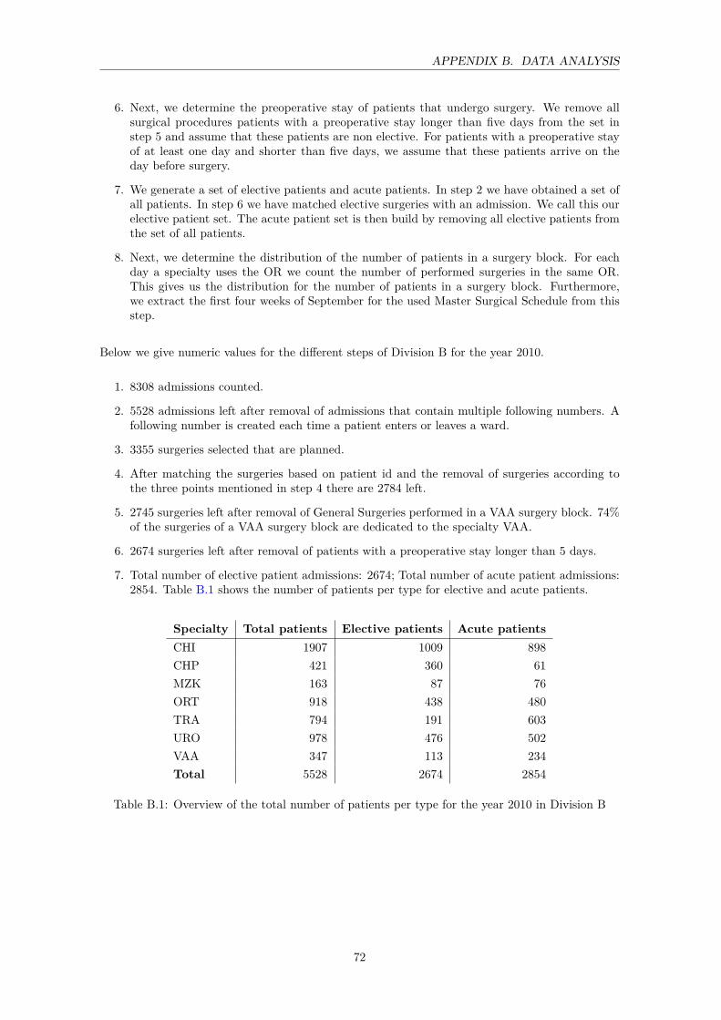
APPENDIX B. DATA ANALYSIS

6. Next, we determine the preoperative stay of patients that undergo surgery. We remove allsurgical procedures patients with a preoperative stay longer than five days from the set instep 5 and assume that these patients are non elective. For patients with a preoperative stayof at least one day and shorter than five days, we assume that these patients arrive on theday before surgery.

7. We generate a set of elective patients and acute patients. In step 2 we have obtained a set ofall patients. In step 6 we have matched elective surgeries with an admission. We call this ourelective patient set. The acute patient set is then build by removing all elective patients fromthe set of all patients.

8. Next, we determine the distribution of the number of patients in a surgery block. For eachday a specialty uses the OR we count the number of performed surgeries in the same OR.This gives us the distribution for the number of patients in a surgery block. Furthermore,we extract the first four weeks of September for the used Master Surgical Schedule from thisstep.

Below we give numeric values for the different steps of Division B for the year 2010.

1. 8308 admissions counted.

2. 5528 admissions left after removal of admissions that contain multiple following numbers. Afollowing number is created each time a patient enters or leaves a ward.

3. 3355 surgeries selected that are planned.

4. After matching the surgeries based on patient id and the removal of surgeries according tothe three points mentioned in step 4 there are 2784 left.

5. 2745 surgeries left after removal of General Surgeries performed in a VAA surgery block. 74%of the surgeries of a VAA surgery block are dedicated to the specialty VAA.

6. 2674 surgeries left after removal of patients with a preoperative stay longer than 5 days.

7. Total number of elective patient admissions: 2674; Total number of acute patient admissions:2854. Table B.1 shows the number of patients per type for elective and acute patients.

Specialty Total patients Elective patients Acute patientsCHI 1907 1009 898CHP 421 360 61MZK 163 87 76ORT 918 438 480TRA 794 191 603URO 978 476 502VAA 347 113 234Total 5528 2674 2854

Table B.1: Overview of the total number of patients per type for the year 2010 in Division B

72

Appendix C

Financial parameters

This appendix is confidential.

73

Appendix D

Class diagram Delphi

Figure D.1: Class diagram of the developed Delphi model

75

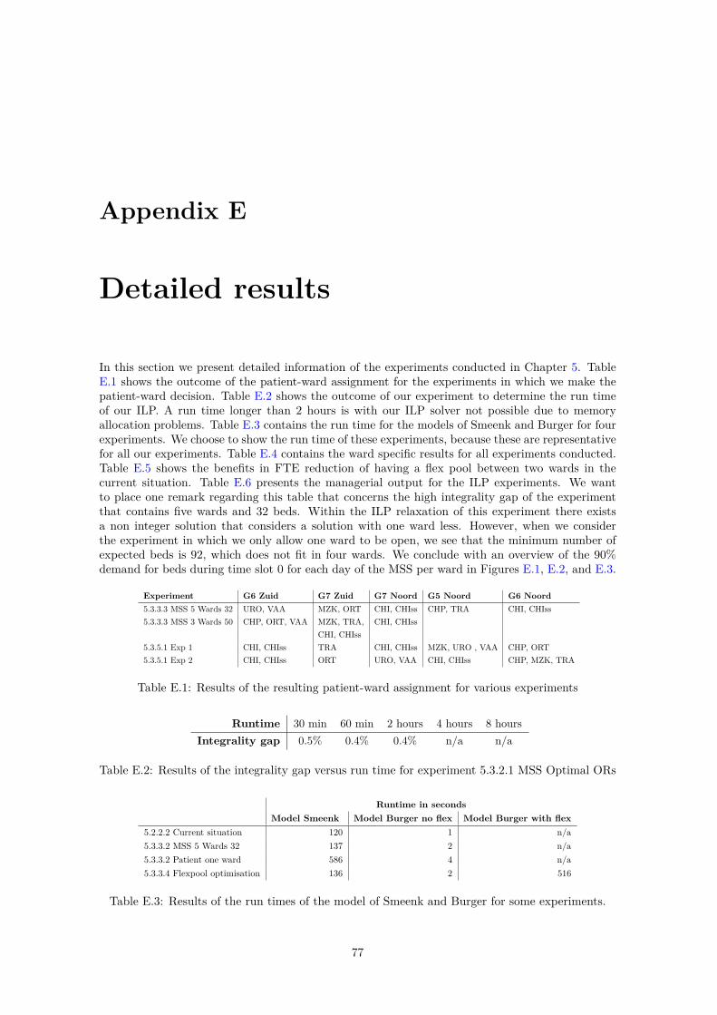
Appendix E

Detailed results

In this section we present detailed information of the experiments conducted in Chapter 5. TableE.1 shows the outcome of the patient-ward assignment for the experiments in which we make thepatient-ward decision. Table E.2 shows the outcome of our experiment to determine the run timeof our ILP. A run time longer than 2 hours is with our ILP solver not possible due to memoryallocation problems. Table E.3 contains the run time for the models of Smeenk and Burger for fourexperiments. We choose to show the run time of these experiments, because these are representativefor all our experiments. Table E.4 contains the ward specific results for all experiments conducted.Table E.5 shows the benefits in FTE reduction of having a flex pool between two wards in thecurrent situation. Table E.6 presents the managerial output for the ILP experiments. We wantto place one remark regarding this table that concerns the high integrality gap of the experimentthat contains five wards and 32 beds. Within the ILP relaxation of this experiment there existsa non integer solution that considers a solution with one ward less. However, when we considerthe experiment in which we only allow one ward to be open, we see that the minimum number ofexpected beds is 92, which does not fit in four wards. We conclude with an overview of the 90%demand for beds during time slot 0 for each day of the MSS per ward in Figures E.1, E.2, and E.3.

Experiment G6 Zuid G7 Zuid G7 Noord G5 Noord G6 Noord5.3.3.3 MSS 5 Wards 32 URO, VAA MZK, ORT CHI, CHIss CHP, TRA CHI, CHIss5.3.3.3 MSS 3 Wards 50 CHP, ORT, VAA MZK, TRA, CHI, CHIss

CHI, CHIss5.3.5.1 Exp 1 CHI, CHIss TRA CHI, CHIss MZK, URO , VAA CHP, ORT5.3.5.1 Exp 2 CHI, CHIss ORT URO, VAA CHI, CHIss CHP, MZK, TRA

Table E.1: Results of the resulting patient-ward assignment for various experiments

Runtime 30 min 60 min 2 hours 4 hours 8 hoursIntegrality gap 0.5% 0.4% 0.4% n/a n/a

Table E.2: Results of the integrality gap versus run time for experiment 5.3.2.1 MSS Optimal ORs

Runtime in secondsModel Smeenk Model Burger no flex Model Burger with flex

5.2.2.2 Current situation 120 1 n/a5.3.3.2 MSS 5 Wards 32 137 2 n/a5.3.3.2 Patient one ward 586 4 n/a5.3.3.4 Flexpool optimisation 136 2 516

Table E.3: Results of the run times of the model of Smeenk and Burger for some experiments.

77

APPENDIX E. DETAILED RESULTS

Minnumberofbeds(90%demand)

Maxnumberofbeds(90%)demand

Averagebedutilisation

Totaldedicatednurses(FTE)

Flexpoolassigned

Averageoverallservicelevelperyear

Averageminimumservicelevelperyear

Minnumberofbeds(90%demand)

Maxnumberofbeds(90%)demand

Averagebedutilisation

Totaldedicatednurses(FTE)

Flexpoolassigned

Averageoverallservicelevelperyear

Averageminimumservicelevelperyear

Minnumberofbeds(90%demand)

Maxnumberofbeds(90%)demand

Averagebedutilisation

Totaldedicatednurses(FTE)

Flexpoolassigned

Averageoverallservicelevelperyear

Averageminimumservicelevelperyear

Minnumberofbeds(90%demand)

Maxnumberofbeds(90%)demand

Averagebedutilisation

Totaldedicatednurses(FTE)

Flexpoolassigned

Averageoverallservicelevelperyear

Averageminimumservicelevelperyear

Minnumberofbeds(90%demand)

Maxnumberofbeds(90%)demand

Averagebedutilisation

Totaldedicatednurses(FTE)

Flexpoolassigned

Averageoverallservicelevelperyear

Averageminimumservicelevelperyear

G6Zuid

G7Zuid

G7Noo

rdG5Noo

rdG6Noo

rd5.2.2.2.

Current

situa

tion

2336

0.65

33.5

10.99

0.92

2034

0.65

26.2

10.99

0.94

1619

0.67

21.7

20.98

0.98

1932

0.61

28.5

0.99

0.94

2131

0.67

30.5

20.99

0.97

Optim

isation

5.3.2.1MSS

Optim

alOrs

2433

0.71

33.1

0.98

0.96

2233

0.67

25.9

0.99

0.96

1519

0.67

21.5

0.98

0.97

2031

0.63

27.0

0.98

0.94

2230

0.69

30.7

1.00

0.99

5.3.2.2MSS

8Ors

2433

0.71

33.3

0.98

0.97

2332

0.69

25.9

0.99

0.98

1520

0.63

21.7

0.99

0.95

1930

0.65

27.1

1.00

0.97

2229

0.72

30.1

0.99

0.98

5.3.3.3MSS

5Wards

3220

300.65

27.2

1.00

0.98

2131

0.67

25.2

0.98

0.97

2130

0.69

30.7

1.00

0.99

1725

0.65

24.5

0.99

0.98

2230

0.71

30.8

1.00

0.99

5.3.3.3MSS

3Wards

5030

430.69

33.6

0.99

0.94

3254

0.65

45.8

0.98

0.88

3448

0.71

45.5

5.3.3.3Pa

tient

oneward

9013

00.76

108.3

0.98

0.91

5.3.3.3MSS

One

ward

9512

70.78

107.1

0.97

0.92

5.3.3.4Flex

pool

optim

isatio

n23

360.65

31.5

0.99

0.92

2034

0.65

24.1

0.99

0.94

1619

0.67

18.5

0.98

0.98

1932

0.61

28.5

0.99

0.94

2131

0.67

29.8

0.99

0.97

5.3.3.5Allcombine

d20

300.65

24.3

10.99

0.89

2131

0.67

23.9

20.97

0.95

2130

0.69

30.7

-1.00

0.99

1725

0.65

22.4

10.99

0.95

2230

0.71

29.8

21.00

0.98

Intervention

s5.3.3.3MSS

leng

th1week

2534

0.71

34.8

0.99

0.97

2432

0.69

25.7

0.99

0.98

1618

0.71

18.6

1.00

1.00

2230

0.69

27.6

1.00

0.99

2330

0.71

30.8

1.00

0.99

5.3.3.3MSS

leng

th2weeks

2633

0.72

33.5

0.98

0.97

2331

0.71

26.0

0.99

0.99

1618

0.71

18.6

1.00

1.00

2131

0.65

27.4

0.98

0.95

2231

0.69

30.9

0.99

0.98

5.3.3.2Steady

cyclic

deman

d22

310.69

30.9

0.99

0.98

1828

0.65

22.5

0.99

0.96

1520

0.62

21.3

0.99

0.95

2030

0.63

26.6

0.99

0.96

2127

0.72

28.9

0.99

0.98

5.3.3.3Increase

20%

2638

0.70

37.0

0.99

0.95

2536

0.69

28.2

0.99

0.95

1620

0.65

22.3

0.99

0.96

2134

0.63

29.7

0.99

0.92

2434

0.70

33.9

0.99

0.96

5.3.3.3Increase

40%

2741

0.72

40.2

0.99

0.96

2640

0.69

30.8

1.00

0.98

1621

0.64

22.4

0.99

0.95

2236

0.64

31.5

0.99

0.93

2636

0.73

35.8

0.99

0.97

5.3.3.4Increase

onepa

tient

increasedde

man

d32

450.73

43.8

0.98

0.95

2740

0.70

30.8

1.00

0.98

1622

0.64

23.8

1.00

0.98

2236

0.65

31.5

0.98

0.93

2940

0.72

39.1

0.99

0.97

5.3.3.4Increase

onepa

tient

norm

alde

man

d25

340.72

34.2

0.99

0.96

2333

0.68

26.1

0.99

0.96

1520

0.64

21.7

0.99

0.95

1932

0.64

29.3

0.99

0.95

2130

0.70

30.8

1.00

0.99

5.3.3.5Size

surgeryblocks

2334

0.69

32.9

0.98

0.94

2133

0.68

25.7

0.99

0.96

1619

0.67

21.7

0.98

0.98

2130

0.67

27.3

1.00

0.98

2230

0.71

30.7

1.00

0.99

5.3.3.6Weekend

surgery

2632

0.73

32.3

0.99

0.99

2431

0.71

25.1

0.99

0.98

1419

0.67

22.0

0.99

0.98

2129

0.67

27.4

1.00

0.99

2329

0.72

30.4

0.99

0.99

5.3.3.7Adm

ission/

Disc

harge

2235

0.66

33.1

0.99

0.93

1834

0.64

26.1

0.99

0.94

1519

0.66

21.3

0.98

0.97

1831

0.62

27.1

0.99

0.93

2030

0.68

30.2

0.99

0.98

5.5.5MSS

leng

th1week3wards

5032

440.70

36.7

0.99

0.96

3748

0.75

44.6

0.99

0.97

3646

0.74

45.9

0.99

0.98

Scen

arios

5.3.4.1LO

S+1currentsit

uatio

n25

400.67

38.3

0.99

0.95

2540

0.66

30.5

1.00

0.98

1722

0.68

24.3

1.00

1.00

2138

0.61

34.0

0.99

0.95

2434

0.70

33.1

0.99

0.95

5.3.4.1LO

S+1MSS

5Wards

3223

340.69

31.6

10.99

0.96

2436

0.68

29.2

20.99

0.95

2334

0.70

33.6

0.99

0.95

2031

0.63

27.1

10.99

0.95

2434

0.71

34.4

20.99

0.96

5.3.4.1LO

S+1Allcombine

d23

340.69

27.9

10.99

0.88

2436

0.68

26.0

20.99

0.93

2334

0.70

33.6

-0.99

0.95

2031

0.63

26.0

10.99

0.93

2434

0.71

29.9

20.99

0.88

5.3.4.1LO

S-1cu

rrentsit

uatio

n21

330.64

31.0

0.99

0.93

1831

0.62

23.9

0.99

0.96

1417

0.66

18.6

1.00

1.00

1729

0.60

25.7

0.99

0.94

2028

0.67

27.3

0.99

0.94

5.3.4.1LO

S-1

MSS

5Wards

3219

270.64

25.4

10.99

0.97

1827

0.67

22.8

20.99

0.97

1928

0.67

27.8

0.99

0.95

1622

0.65

21.5

11.00

0.99

2028

0.68

28.5

20.99

0.97

5.3.4.1LO

S-1

Allcombine

d19

270.64

24.3

10.99

0.99

1827

0.67

20.5

20.99

0.94

1928

0.67

27.8

0.99

0.95

1622

0.65

18.6

10.99

0.92

2028

0.68

24.1

20.99

0.86

5.3.4.2Acute-25%

currentsit

uatio

n20

330.64

31.1

0.99

0.93

1831

0.63

24.0

0.99

0.96

1115

0.62

17.9

0.99

0.99

1628

0.59

25.0

0.99

0.94

1928

0.66

27.2

0.99

0.94

5.3.4.2Acute-25%

MSS

5Wards

3217

250.66

24.3

11.00

1.00

1828

0.64

22.8

20.99

0.96

1927

0.69

27.7

0.99

0.96

1320

0.63

19.1

11.00

0.98

1927

0.71

28.1

20.99

0.97

5.3.4.2Acute-25%

Allcombine

d17

250.66

24.3

11.00

1.00

1828

0.64

20.5

20.99

0.90

1927

0.69

27.7

0.99

0.96

1320

0.63

16.7

10.99

0.93

1927

0.71

23.6

20.96

0.87

5.3.4.2Acute+25

%cu

rrentsit

uatio

n25

380.66

35.5

0.99

0.92

2236

0.65

27.6

0.99

0.93

1721

0.67

24.3

1.00

1.00

2135

0.62

30.0

0.99

0.91

2332

0.69

31.4

0.99

0.97

5.3.4.2Acute+25

%MSS

5Wards

3222

320.67

29.9

10.99

0.96

2333

0.68

27.3

20.99

0.96

2332

0.69

31.6

0.99

0.97

1826

0.67

24.9

10.99

0.98

2332

0.71

31.8

20.99

0.98

5.3.4.2Acute+25

%Allcombine

d22

320.67

27.7

10.97

0.93

2333

0.68

24.1

20.99

0.90

2332

0.69

31.6

0.99

0.97

1826

0.67

22.2

10.98

0.91

2332

0.71

29.8

20.99

0.94

Param

eters

5.3.5.1ILP

Exp1

2230

0.71

30.8

1.00

0.99

1619

0.67

21.5

0.98

0.97

2130

0.69

30.8

1.00

0.99

2235

0.62

30.7

0.99

0.92

2332

0.69

25.7

0.99

0.98

5.3.5.1ILP

Exp2

2230

0.71

30.8

1.00

0.99

1828

0.66

22.8

1.00

0.97

2131

0.63

27.1

0.98

0.94

2130

0.69

30.7

1.00

0.99

1927

0.68

25.7

1.00

0.99

5.3.5.2Se

rvlvls

Exp1.

nofle

x23

360.65

31.7

0.96

0.88

2034

0.65

24.3

0.96

0.91

1619

0.67

18.6

0.94

0.95

1932

0.61

27.9

0.98

0.94

2131

0.67

29.8

0.98

0.96

5.3.5.2Se

rvlvls

Exp1.

flex

2336

0.65

31.7

0.96

0.88

2034

0.65

24.3

0.96

0.91

1619

0.67

18.6

0.94

0.95

1932

0.61

27.9

0.98

0.94

2131

0.67

29.8

0.98

0.96

5.3.5.2Se

rvlvls

Exp2.

nofle

x23

360.65

30.8

0.95

0.86

2034

0.65

22.9

0.94

0.86

1619

0.67

18.6

0.94

0.95

1932

0.61

25.0

0.94

0.85

2131

0.67

26.5

0.91

0.85

5.3.5.2Se

rvlvls

Exp2.

flex

2336

0.65

29.8

0.94

0.83

2034

0.65

20.6

0.90

0.78

1619

0.67

15.0

0.91

0.79

1932

0.61

25.0

0.94

0.85

2131

0.67

24.1

0.90

0.77

5.3.5.2Se

rvlvls

Exp3.

nofle

x23

360.65

30.8

0.95

0.86

2034

0.65

22.9

0.94

0.86

1619

0.67

18.6

0.94

0.95

1932

0.61

25.0

0.94

0.85

2131

0.67

26.5

0.91

0.85

5.3.5.2Se

rvlvls

Exp3.

flex

2336

0.65

29.8

10.94

0.83

2034

0.65

20.6

10.90

0.78

1619

0.67

15.0

20.91

0.79

1932

0.61

25.0

0.94

0.85

2131

0.67

24.1

20.90

0.77

5.3.5.2Pa

tient-to-nu

rseratio

noflex

2336

0.65

31.1

0.99

0.91

2034

0.65

30.4

0.99

0.93

1619

0.67

18.6

1.00

1.00

1932

0.61

28.5

0.99

0.94

2131

0.67

27.9

0.98

0.96

5.3.5.2Pa

tient-to-nu

rseratio

flex

2336

0.65

27.7

10.97

0.82

2034

0.65

27.7

10.98

0.87

1619

0.67

18.6

1.00

1.00

1932

0.61

27.9

20.99

0.94

2131

0.67

24.4

20.98

0.86

TableE.4:

Detailedman

agerialinformationpe

rwardforeach

expe

riment

78

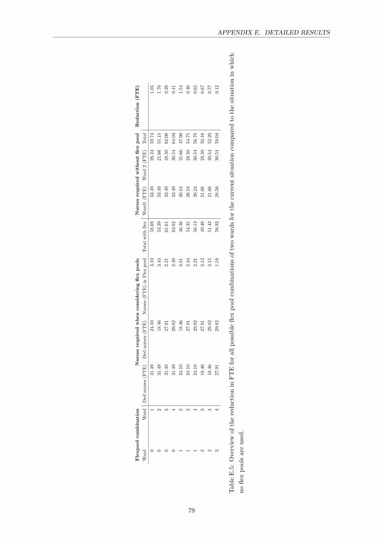
APPENDIX E. DETAILED RESULTS

Flexp

oolcombina

tion

Nursesrequ

ired

whe

nconsideringfle

xpo

ols

Nursesrequ

ired

witho

utfle

xpo

olRed

uction

(FTE)

Ward

Ward

Ded

nurses

(FTE)

Ded

nurses

(FTE)

Nurses(F

TE)

inFlex

pool

Totalw

ithfle

xWard1

(FTE)

Ward2(F

TE)

Total

01

31.49

24.10

3.10

58.69

33.49

26.24

59.74

1.05

02

31.49

18.46

3.44

53.39

33.49

21.66

55.15

1.76

03

31.49

27.91

2.21

61.61

33.49

28.50

62.00

0.39

04

31.49

29.82

2.30

63.62

33.49

30.54

64.03

0.41

12

24.10

18.46

3.81

46.36

26.24

21.66

47.90

1.54

13

24.10

27.91

2.34

54.35

26.24

28.50

54.75

0.40

14

24.10

29.82

2.21

56.13

26.24

30.54

56.78

0.65

23

18.46

27.91

3.12

49.49

21.66

28.50

50.16

0.67

24

18.46

29.82

3.15

51.43

21.66

30.54

52.20

0.77

34

27.91

29.82

1.18

58.92

28.50

30.54

59.04

0.12

TableE.5:

Overview

oftheredu

ctionin

FTEforallp

ossib

lefle

xpo

olcombina

tions

oftw

owards

forthecu

rrents

ituationcompa

redto

thesit

uatio

nin

which

nofle

xpo

olsareused

.

79

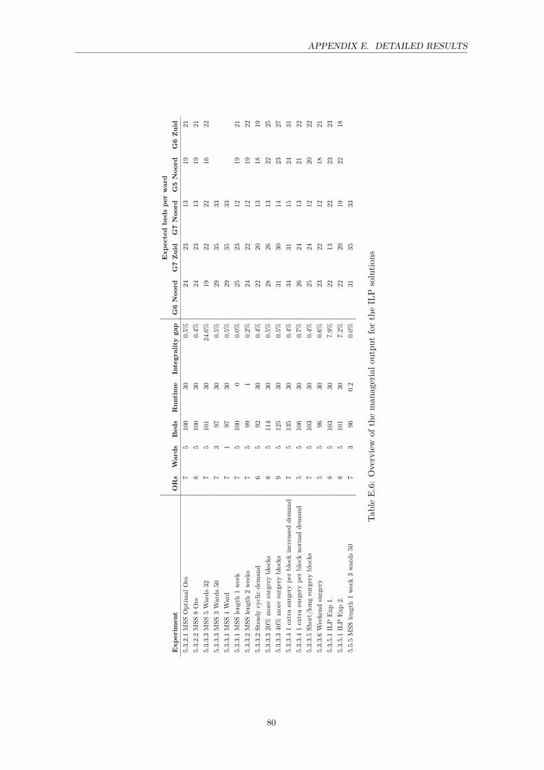
APPENDIX E. DETAILED RESULTS

Exp

ectedbe

dspe

rward

Exp

erim

ent

ORs

Wards

Bed

sRun

time

Integralitygap

G6Noo

rdG7Zuid

G7Noo

rdG5Noo

rdG6Zuid

5.3.2.1MSS

Optim

alOrs

75

100

300.5%

2423

1319

215.3.2.2MSS

8Ors

85

100

300.4%

2423

1319

215.3.3.3MSS

5Wards

327

5101

3024.6%

1922

2216

225.3.3.3MSS

3Wards

507

397

300.5%

2935

335.3.3.1MSS

1Ward

71

9730

0.5%

2935

335.3.3.1MSS

leng

th1week

75

100

00.0%

2523

1219

215.3.3.2MSS

leng

th2weeks

75

991

0.2%

2422

1219

225.3.3.2Steady

cyclic

deman

d6

592

300.4%

2220

1318

195.3.3.320%

moresurgeryblocks

85

114

300.5%

2826

1322

255.3.3.340%

moresurgeryblocks

95

125

300.5%

3130

1423

275.3.3.41extrasurgerype

rblockincreasedde

man

d7

5135

300.4%

3431

1524

315.3.3.41extrasurgerype

rblockno

rmal

deman

d5

5106

300.7%

2624

1321

225.3.3.5Sh

ort/long

surgeryblocks

75

103

300.4%

2524

1220

225.3.3.6Weekend

surgery

55

9630

0.6%

2322

1218

215.3.5.1ILP

Exp1.

85

103

307.9%

2213

2223

235.3.5.1ILP

Exp2.

85

101

307.2%

2220

1922

185.5.5MSS

leng

th1week3wards

507

396

0.2

0.0%

3135

33

TableE.6:

Overview

oftheman

agerialo

utpu

tfortheILP

solutio

ns

80

APPENDIX E. DETAILED RESULTS

(a) G6 Zuid

(b) G7 Zuid

(c) G7 Noord

(d) G5 Noord

(e) G6 Noord

Figure E.1: 90% demand for beds for each day of the MSS at time slot 0, experiment 5.2.2.2 Currentsituation

81

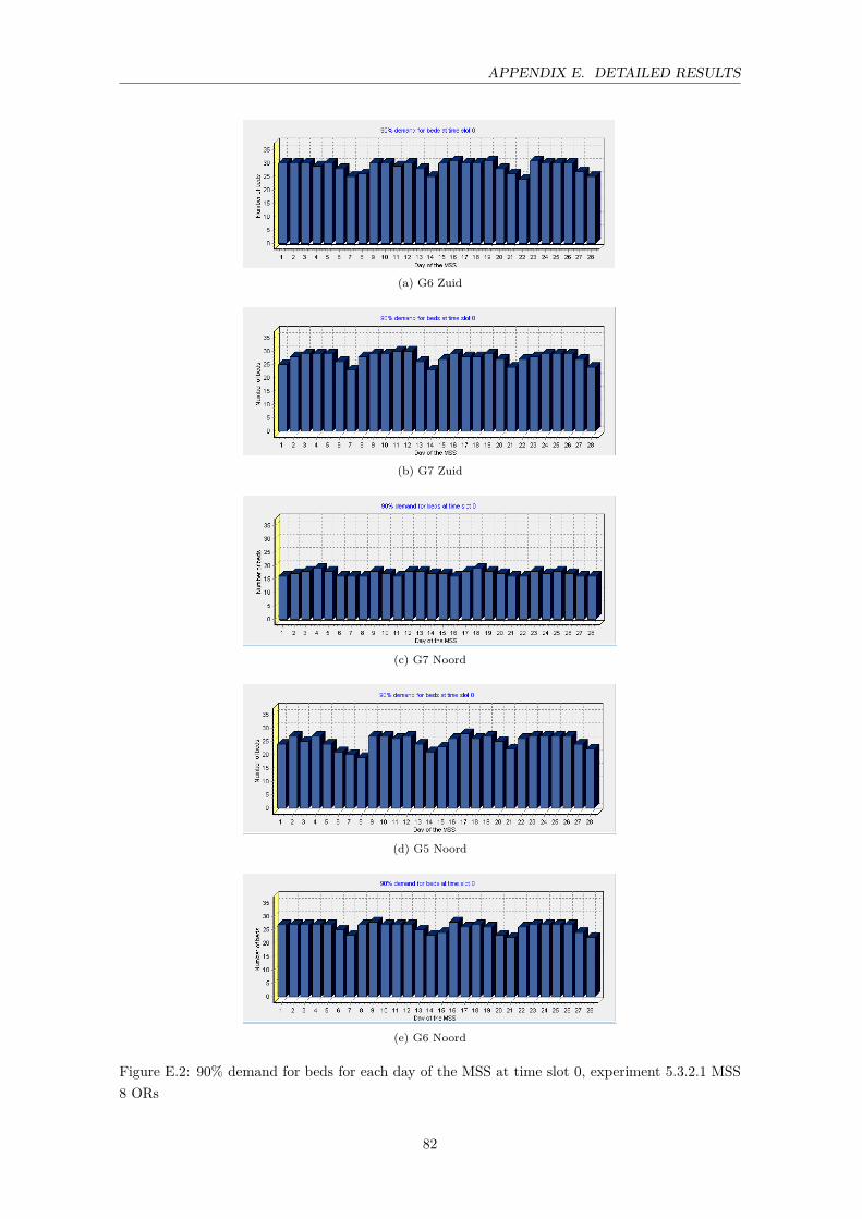
APPENDIX E. DETAILED RESULTS

(a) G6 Zuid

(b) G7 Zuid

(c) G7 Noord

(d) G5 Noord

(e) G6 Noord

Figure E.2: 90% demand for beds for each day of the MSS at time slot 0, experiment 5.3.2.1 MSS8 ORs

82

APPENDIX E. DETAILED RESULTS

(a) G6 Zuid

(b) G7 Zuid

(c) G7 Noord

(d) G5 Noord

(e) G6 Noord

Figure E.3: 90% demand for beds for each day of the MSS at time slot 0, experiment 5.3.3.6.weekend surgery

83