RESPIRE: Robust SEnSor Placement OptImizationin PRobabilistic Environments

Onat Gungor1,3, Tajana S. Rosing2, and Baris Aksanli3

1Department of Electrical and Computer Engineering, University of California San Diego2Department of Computer Science and Engineering, University of California San Diego

3Department of Electrical and Computer Engineering, San Diego State Universityogungor@ucsd.edu, tajana@ucsd.edu, baksanli@sdsu.edu

Abstract—Optimal sensor coverage considers where to placesensors at minimal cost while maximizing coverage. This ap-proach often overlooks the robustness of the entire system. Ifsensors break down, the application performance might severelybe affected. This paper constructs a multi-objective optimiza-tion model that considers not only optimal coverage, but alsorobustness. Our method increases the system robustness by upto 50% compared to a coverage-only approach with 201% higherprobability of monitoring the entire environment.

I. INTRODUCTION AND RELATED WORK

Sensor placement directly impacts the efficiency of theallocated resources and system performance [1], consideringcoverage and connectivity [2]. For the best performance,applications should observe and monitor the greatest totalrelevant area possible, i.e. high coverage. Previous studiesoptimize sensor coverage, with the goal of maximizing sensorcoverage with minimum sensor cost [3], [4], energy consump-tion [5], or communication bandwidth [6]. Solutions to theseoptimization problems include [7] [8]: 1) Exhaustive searchconsiders all possible locations for sensor placement [9], whichhas exponential complexity. 2) Optimization-based approachesconstruct integer programming models which can be solved byconventional solvers, [10]–[12]. but may not obtain a solutionin polynomial time. 3) Heuristics try to find nearly optimalsolution(s) with reasonable execution time [13]–[17].

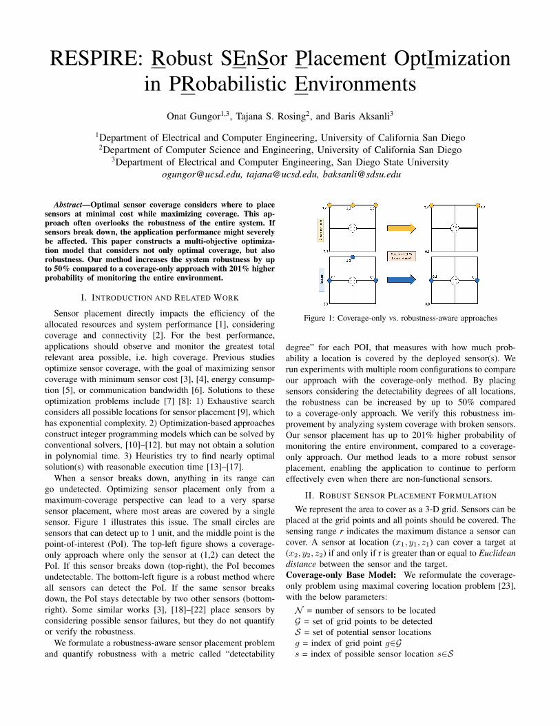
When a sensor breaks down, anything in its range cango undetected. Optimizing sensor placement only from amaximum-coverage perspective can lead to a very sparsesensor placement, where most areas are covered by a singlesensor. Figure 1 illustrates this issue. The small circles aresensors that can detect up to 1 unit, and the middle point is thepoint-of-interest (PoI). The top-left figure shows a coverage-only approach where only the sensor at (1,2) can detect thePoI. If this sensor breaks down (top-right), the PoI becomesundetectable. The bottom-left figure is a robust method whereall sensors can detect the PoI. If the same sensor breaksdown, the PoI stays detectable by two other sensors (bottom-right). Some similar works [3], [18]–[22] place sensors byconsidering possible sensor failures, but they do not quantifyor verify the robustness.

We formulate a robustness-aware sensor placement problemand quantify robustness with a metric called “detectability

Figure 1: Coverage-only vs. robustness-aware approaches

degree” for each POI, that measures with how much prob-ability a location is covered by the deployed sensor(s). Werun experiments with multiple room configurations to compareour approach with the coverage-only method. By placingsensors considering the detectability degrees of all locations,the robustness can be increased by up to 50% comparedto a coverage-only approach. We verify this robustness im-provement by analyzing system coverage with broken sensors.Our sensor placement has up to 201% higher probability ofmonitoring the entire environment, compared to a coverage-only approach. Our method leads to a more robust sensorplacement, enabling the application to continue to performeffectively even when there are non-functional sensors.

II. ROBUST SENSOR PLACEMENT FORMULATION

We represent the area to cover as a 3-D grid. Sensors can beplaced at the grid points and all points should be covered. Thesensing range r indicates the maximum distance a sensor cancover. A sensor at location (x1, y1, z1) can cover a target at(x2, y2, z2) if and only if r is greater than or equal to Euclideandistance between the sensor and the target.Coverage-only Base Model: We reformulate the coverage-only problem using maximal covering location problem [23],with the below parameters:N = number of sensors to be locatedG = set of grid points to be detectedS = set of potential sensor locationsg = index of grid point g∈Gs = index of possible sensor location s∈S

r = sensor sensing rangedsg = euclidean distance between sensor and grid pointξsg = 1 if dsg ≤ r; 0 otherwise

The decision variables are as follows:Xs = 1 if sensor is positioned at location s; 0 otherwiseYg = 1 if grid point g is detected; 0 otherwiseThe integer linear programming (ILP) model becomes:

maximize∑g∈G

Yg (1)

subject to∑s∈S

ξsgXs ≥ Yg ∀g ∈ G (2)

∑s∈S

Xs = N (3)

Xs = {0, 1} ∀s ∈ S, Yg = {0, 1} ∀g ∈ G (4)

(1) is the objective function which maximizes the numberof grid points covered. Constraints (2) enable a grid point gto be covered if and only if one or more sensors can detect it.Constraint (3) forces to place exactly N sensors. Constraints(4) are binary variable constraints for the decision variables.Coverage-only Probabilistic Model: The base coverage-only model assumes that a sensor can only make binarydetection decisions. In reality, there is an uncertainty withsensor readings. Thus, sensor detection should be based ona probabilistic model [24], e.g. with respect to the distancebetween a sensor and a point. To achieve this, we define psgas the detection probability of a point g by sensor at point s.We use a common function [25] for the relationship betweendsg and psg: psg = e−αdsg where α denotes the rate at whichsensor’s detection probability decreases with distance. Withlarger α, psg decreases quicker with distance.

We calculate psg values for all possible sensor-grid pointtuples using the above function. We denote the probability ofmissing a grid point g with a sensor located at s as 1−psgXs.We use τg as the maximum allowable miss probability for eachpoint (between 0 and 1). Larger τg leads to full coverage withfewer sensors (flexible system), whereas smaller τg requiresmore sensors to obtain full coverage (strict system). Wereformulate constraints (2) as:∑

s∈SηsgXs ≥ ζgYg ∀g ∈ G (5)

where ηsg = − ln(1 − psg) and ζg = − ln(τg). Here, themeaning of Yg changes from before, where it measures thenumber of points that satisfy constraints (5).Robustness-Aware Probabilistic Model: In a sensor net-work, each sensor may not correctly and accurately functionindefinitely. There might be some environmental disruptionswhich affect the working condition of a sensor, leading tomalfunctioning, inaccurate readings, or a complete breakingdown. To prevent this, we need to place the sensors in away to increase the resilience of the system. We constructa robust sensor placement model with probabilistic detection.

We define “detectability degree” (δg) as the sum of detectionprobabilities from placed sensors to each point:

δg =∑s∈S

psgXs ∀g ∈ G (6)

To understand this formulation better, consider Figure 1where sensor detection is binary (psg is 1 if detected, otherwiseit is 0). In the top-left figure, δg is 1, whereas in bottom-leftit is three (i.e. the point can be detected by three sensors.)In our case, instead of binary numbers (0 or 1), we usedetection probabilities to find δg . We define the robustnessof a system using average (µ) and minimum (ψ) δg . (10) and(11) provide mathematical formulations for these variables.For a location, higher detectability degree means a more robustsystem because if some sensor(s) covering that point breakdown, there are alternatives to cover that particular point.

We provide a simple sensor placement scenario to explainthese values in more detail. Assume that we have five points todetect and seven sensors with binary sensor detection, where{2, 5, 6, 7, 0} gives us the number of sensors that candetect each point (i.e. first point is detected by two sensors,etc.) In this set, the average detection value is 4 (20/5), withminimum as 0. Even though the average value is high, thereare still points with significantly low values, thus making thesystem vulnerable to sensor break downs. Thus, we need toconsider both the average and minimum values to obtain amore equally distributed set. For our formulation, we replacethe number of sensors with detection probabilities. Below isthe multi-objective optimization model with weighted sumsfor the average and minimum values [26]:

maximize w1µ+ w2ψ (7)

subject to∑s∈S

ηsgXs ≥ ζg ∀g ∈ G (8)

∑s∈S

Xs = N (9)

µ =

∑g∈G

∑s∈S psgXs

|G|(10)

ψ ≤∑s∈S

psgXs ∀g ∈ G (11)

w1 + w2 = 1 (12)

(7) is our objective function which maximizes the sum ofaverage and minimum detectablity degrees. Constraints (8) arethe probabilistic constraints where ηsg = − ln(1−psg) and ζg= − ln(τg). Constraint (9) forces to place exactly N number ofsensors. Constraint (10) is an equality constraint for averagedetectability degree where |G| denotes cardinality of set G.Constraint (11) is another equality constraint which denotesminimum detectability degree. Constraint (12) forces sum ofweights to be equal to 1. In our model, we select the valuesof w1 and w2 as 0.5, i.e. we assign equal importance to theaverage and minimum detectability degrees.

Table I: Minimum (average) value improvement with 1 broken sensor

# Sensors Small Medium Large Very Large15 38% (2.7%) 67% (5.4%) 33% (5.9%) 26% (7.8%)20 196% (0.9%) 146% (0.4%) 101% (3.7%) 82% (7.2%)25 146% (0.5%) 180% (0.8%) 126% (1.7%) 108% (4.9%)30 79% (-0.2%) 201% (0.8%) 131% (0.7%) 94% (7.4%)

III. EVALUATION

Experimental Setup: We implement ILP models in CPLEX12.10 [27] and run experiments on a PC with 16 GB RAMand an 8-core 2.3 GHz Intel Core i9 processor. We adoptthe setup from [28] with low-resolution thermal sensors. Weconsider different room configurations with a fixed height of3m [29]. The distance between each point is 1.5m. Sensors canbe placed on each point and all points should be covered bya sensor. Some points are not feasible for sensor placement,e.g. some middle points (as a sensor cannot be placed inthe air). The room settings are: 1) small: 4.5m×4.5m×3m,2) medium: 6m×6m×3m, 3) large: 7.5m×7.5m ×3m, 4) verylarge: 9m×9m×3m. We use a τg value of 0.4 for the smallroom and increase it by 0.05 for each larger setting. Weexperimentally determine these τg values to provide a balancedsensor placement. To find the optimal value of α, we performan experiment to measure the probability of detecting a personwith respect to increasing distance. We use curve-fitting on themeasured values and obtain the optimal α as 0.576.Results: The left hand side (LHS) of Equation 8 for eachpoint indicates how well the point is covered. As the LHSgets bigger, the point is covered with higher probability,less prone to sensor break downs. To illustrate robustness,we create a scenario where one sensor breaks down. Wecalculate the LHS values of Equation 8 for each point forboth coverage-only [3], [30] and robustness-aware models.We calculate the minimum and average LHS values acrossall grid points, excluding the broken sensor. The minimumvalue shows the most vulnerable point, while the averagemeasures the vulnerability across all points. Figure 2 showsthis in detail for the small room with 4 cases, 15 and 30sensors in a); 20 and 25 sensors in b). For each case, wecalculate the minimum LHS value across all points when aparticular sensor breaks down, for both coverage-only androbust models. The X-axis indicates different broken sensors,i.e. each blue (robust)/yellow (coverage-only) column pairrepresents a broken sensor. For each case, the right-most twocolumns represent no broken sensor case. Our model leadsto significantly higher minimum LHS values when a sensorbreaks down, i.e. the most vulnerable point with our modelhas a much higher probability of detection as compared to thecoverage-only case, hence less prone to broken sensors.

We expand this analysis on all room settings with 15, 20,25, and 30 sensors, comparing the minimum (average) LHSvalue improvement of our method in Table I. The averageand minimum value changes are up to 7.8% and 201%,respectively. The minimum value is more important as it showsthe most vulnerable point and our method makes the mostvulnerable point significantly less prone to broken sensors.

(a) 15 & 30 sensors

(b) 20 & 25 sensors

Figure 2: Small room min detectability degree: Coverage-only [3],[30] vs. Our Robust Model (a) 15-30 sensors (b) 20-25 sensors

Figure 3: Reliability improvement vs. number of sensors

Next, we calculate Equation 7 to quantify the robustnessof a sensor placement, across all room settings with differentnumber of sensors in Figure 3. The maximum robustness im-provement is 50% in medium room with 30 sensors. Averageimprovement is 32%, 41%, 31%, and 31% for small, medium,large, and very large rooms, respectively.

IV. CONCLUSION

Sensors are prone to breaking, thus performance of asensor-based application can be heavily impacted by missingsensors. We propose a new robustness-aware and probabilisticsensor placement method to maintain the coverage of a sensorfield even with missing sensors. Our method increases therobustness of a sensor-based system by up to 50% compared toa coverage-only approach, with up to 201% higher probabilityof monitoring the entire area, even with broken sensors.

ACKNOWLEDGEMENT

This work has been funded in part by NSF, with awardnumbers #1830331, #1911095, #1826967, #1730158, and#1527034. It was also partially supported by SRC task#2805.001.

REFERENCES

[1] A. T. Murray, K. Kim, J. W. Davis, R. Machiraju, and R. Parent,“Coverage optimization to support security monitoring,” Computers,Environment and Urban Systems, vol. 31, no. 2, pp. 133–147, 2007.

[2] H. Xu, J. Zhu, and B. Wang, “On the deployment of a connected sensornetwork for confident information coverage,” Sensors, vol. 15, no. 5,pp. 11277–11294, 2015.

[3] M. P. Fanti, M. Roccotelli, G. Faraut, and J.-J. Lesage, “Smart placementof motion sensors in a home environment,” in 2017 IEEE InternationalConference on Systems, Man, and Cybernetics (SMC), pp. 894–899,IEEE, 2017.

[4] O. Moh’d Alia and A. Al-Ajouri, “Maximizing wireless sensor networkcoverage with minimum cost using harmony search algorithm,” IEEESensors Journal, vol. 17, no. 3, pp. 882–896, 2016.

[5] C. Yang and K.-W. Chin, “On nodes placement in energy harvestingwireless sensor networks for coverage and connectivity,” IEEE Trans-actions on Industrial Informatics, vol. 13, no. 1, pp. 27–36, 2016.

[6] Y. Pei and M. W. Mutka, “Joint bandwidth-aware relay placementand routing in heterogeneous wireless networks,” in 2011 IEEE 17thInternational Conference on Parallel and Distributed Systems, pp. 420–427, IEEE, 2011.

[7] A. Maheshwari and N. Chand, “A survey on wireless sensor networkscoverage problems,” in Proceedings of 2nd International Conferenceon Communication, Computing and Networking, pp. 153–164, Springer,2019.

[8] B. Wang, “Coverage problems in sensor networks: A survey,” ACMComputing Surveys (CSUR), vol. 43, no. 4, pp. 1–53, 2011.

[9] F. Y. Lin and P.-L. Chiu, “A near-optimal sensor placement algorithmto achieve complete coverage-discrimination in sensor networks,” IEEECommunications Letters, vol. 9, no. 1, pp. 43–45, 2005.

[10] I. Vlasenko, I. Nikolaidis, and E. Stroulia, “The smart-condo: Optimiz-ing sensor placement for indoor localization,” IEEE Transactions onSystems, Man, and Cybernetics: Systems, vol. 45, no. 3, pp. 436–453,2014.

[11] M. P. Fanti, G. Faraut, J.-J. Lesage, and M. Roccotelli, “An integratedframework for binary sensor placement and inhabitants location track-ing,” IEEE Transactions on Systems, Man, and Cybernetics: Systems,vol. 48, no. 1, pp. 154–160, 2016.

[12] L. Sela and S. Amin, “Robust sensor placement for pipeline monitoring:Mixed integer and greedy optimization,” Advanced Engineering Infor-matics, vol. 36, pp. 55–63, 2018.

[13] A. N. Njoya, C. Thron, J. Barry, W. Abdou, E. Tonye, N. S. L. Konje,and A. Dipanda, “Efficient scalable sensor node placement algorithmfor fixed target coverage applications of wireless sensor networks,” IETWireless Sensor Systems, vol. 7, no. 2, pp. 44–54, 2017.

[14] Y. Chae and D. N. Wilke, “Heuristic linear algebraic rank-varianceformulation and solution approach for efficient sensor placement,”Engineering Structures, vol. 153, pp. 717–731, 2017.

[15] J. A. Grant, A. Boukouvalas, R.-R. Griffiths, D. S. Leslie, S. Vakili,and E. M. De Cote, “Adaptive sensor placement for continuous spaces,”arXiv preprint arXiv:1905.06821, 2019.

[16] R. Hou, Y. Xia, Q. Xia, and X. Zhou, “Genetic algorithm based opti-mal sensor placement for l1-regularized damage detection,” StructuralControl and Health Monitoring, vol. 26, no. 1, p. e2274, 2019.

[17] M. R. Senouci and A. Abdellaoui, “Efficient sensor placement heuris-tics,” in 2017 IEEE International Conference on Communications (ICC),pp. 1–6, IEEE, 2017.

[18] C. Yang, K.-W. Chin, Y. Liu, J. Zhang, and T. He, “Robust targets cover-age for energy harvesting wireless sensor networks,” IEEE Transactionson Vehicular Technology, vol. 68, no. 6, pp. 5884–5892, 2019.

[19] R. Mohan and B. de Jager, “Robust optimal sensor planning forocclusion handling in dynamic robotic environments,” IEEE SensorsJournal, vol. 19, no. 11, pp. 4259–4270, 2019.

[20] M. Erdelj, N. Mitton, and T. Razafindralambo, “Robust wireless sensornetwork deployment,” 2016.

[21] K. Vu and R. Zheng, “Robust coverage under uncertainty in wirelesssensor networks,” in 2011 Proceedings IEEE INFOCOM, pp. 2015–2023, IEEE, 2011.

[22] K. Xu, G. Takahara, and H. Hassanein, “On the robustness of grid-based deployment in wireless sensor networks,” in Proceedings of the2006 international conference on Wireless communications and mobilecomputing, pp. 1183–1188, 2006.

[23] O. Karasakal and E. K. Karasakal, “A maximal covering location modelin the presence of partial coverage,” Computers & Operations Research,vol. 31, no. 9, pp. 1515–1526, 2004.

[24] R. R. Brooks and S. S. Iyengar, Multi-sensor fusion: fundamentals andapplications with software. Prentice-Hall, Inc., 1998.

[25] S. S. Dhillon, K. Chakrabarty, and S. S. Iyengar, “Sensor placement forgrid coverage under imprecise detections,” in Proceedings of the FifthInternational Conference on Information Fusion. FUSION 2002.(IEEECat. No. 02EX5997), vol. 2, pp. 1581–1587, IEEE, 2002.

[26] R. T. Marler and J. S. Arora, “The weighted sum method for multi-objective optimization: new insights,” Structural and multidisciplinaryoptimization, vol. 41, no. 6, pp. 853–862, 2010.

[27] C. U. Manual, “Ibm ilog cplex optimization studio,” Version, vol. 12,pp. 1987–2018, 1987.

[28] S. Shelke and B. Aksanli, “Static and dynamic activity detection withambient sensors in smart spaces,” Sensors, vol. 19, no. 4, p. 804, 2019.

[29] M. I. Hamakareem, “Minimum height and size standards for roomsin buildings.” URL: https://theconstructor.org/building/rooms-minimum-height-size-standards/5116/, Nov 2018.

[30] I. K. Altınel, N. Aras, E. Guney, and C. Ersoy, “Binary integerprogramming formulation and heuristics for differentiated coverage inheterogeneous sensor networks,” Computer Networks, vol. 52, no. 12,pp. 2419–2431, 2008.