RESPONSE OF RIPARIAN COTTONWOODS

TO EXPERIMENTAL FLOWS ALONG THE LOWER BRIDGE RIVER,

BRITISH COLUMBIA

ALEXIS ANNE HALL Bachelor of Science, University of Lethbridge, 2004

A Thesis Submitted to the School of Graduate Studies of the

University of Lethbridge in Partial fulfilment of the requirements for the Degree

MASTER OF SCIENCE

Department of Biological Sciences University of Lethbridge

LETHBRIDGE, ALBERTA, CANADA

© Alexis A. Hall, 2007

Abstract The Bridge River drains the east slope of the Coast Mountain Range and is a

major tributary of the Fraser River in southwestern British Columbia. The lower

Bridge River has been regulated since the installation of Terzaghi Dam in 1948,

which left a section of dry riverbed for an interval of 52 years prior to 2000. An

out-of-court settlement between BC Hydro and Federal and Provincial Fisheries

regulatory agencies resulted in the required experimental discharge of 3 m3/s

below Terzaghi Dam in 2000. This study investigated growth of black

cottonwood (Populus trichocarpa) trees in response to the experimental

discharges. Mature trees did not show a significant response in radial trunk

growth or branch elongation. In contrast, the juvenile trees displayed an increased

growth response, and the successful establishment of saplings provided a dramatic

response to the new flow regime. Thus, I conclude that cottonwoods have

benefited from the experimental flow regime of the lower Bridge River.

iii

Preface – Thesis Structure This research-based MSc. thesis has two chapters and five appendices.

Chapter 1 provides an introduction to the Bridge River valley, with a historic look

at hydroelectric power generation, mining and a brief description of vegetation

and wildlife.

Chapter 2 is a stand-alone research paper summing up my research, which

includes field samples from 2003-2007 used to analyze the growth and

recruitment of riparian cottonwood trees along the lower Bridge River, British

Columbia.

Appendix 1: Yalakom River regression analysis

Appendix 2: Vegetation Index

Appendix 3: Birds and Mammals Index

Appendix 4: Fishes Index

Appendix 5: T-test results for Figure 2.12.

iv

Acknowledgements I would like to extend my heartfelt thanks to Dr. Stewart Rood, for all the years of

encouragement and support he has given me throughout. His endless enthusiasm

fuelled my studies of the wonders of riparian zones and rivers.

I would like to thank Paul Higgins for his wealth of knowledge about the Bridge

River, data and insight. Thank you to David Pearce for spending days upon days

helping me determine the best possible way to measure basal area, and having the

patience to try all of them. Thank you to my committee members: Hester Jiskoot

and Joseph Rasmussen, for supporting me throughout.

I would like to thank the girls in the lab: Colleen, Karen and Julie (the cottonwood

team) for their help, encouragement and hours of thoughtful contemplation. I

would like to thank Colleen for sitting beside me and putting up with me every

day, all day, and night for two years. Thank you to Karen for teaching me

hydrology more than once, and to Julie for helping with editing.

I could not have collected all the data I did without all the support from my trusty

field assistants: Breanne Patterson, Steven Hall, Brett Weisser, and Riley Hall,

along with the faithful hounds Otter, Max and Kismet.

The Bridge River is a river that I will think about for many years to come.

v

Table of contents

Signature page .................................................................................................. ii

Abstract .............................................................................................................. iii

Preface................................................................................................................ iv

Acknowledgements ........................................................................................... v

Table of Contents............................................................................................... vi

List of Tables .................................................................................................... viii

List of Figures ................................................................................................... ix

Abbreviations .................................................................................................... xii

Chapter 1: River damming and hydroelectric power production in the

Bridge River valley ......................................................................................... 1

1.1 Introduction ................................................................................................. 1

1.2 Natural History ............................................................................................ 9

1.3 Geography ................................................................................................... 13

1.4 Human History ............................................................................................ 15

1.5 BC Hydro controlled flow experiment ....................................................... 16

1.6 The Bridge River today................................................................................ 17

1.7 My thesis research........................................................................................ 18

1.8 Conclusion .................................................................................................. 19

vi

Chapter 2: Response of riparian cottonwoods to experimental flows along

the lower Bridge River, British Columbia. ................................................... 20

2.1 Introduction ................................................................................................. 20

2.1.1 Life history and ecophysiology of black cottonwoods ............................ 23

2.1.2 The lower Bridge River ........................................................................... 25

2.1.3 The Bridge River today ............................................................................ 26

2.1.4 This study ................................................................................................. 30

2.2 Methods ....................................................................................................... 31

2.2.1 Hydrology ................................................................................................ 31

2.2.2 Mature trees ............................................................................................. 35

2.2.3 Juveniles ................................................................................................... 39

2.2.4 Saplings .................................................................................................... 43

2.3 Results ......................................................................................................... 44

2.3.1 Hydrology ................................................................................................ 44

2.3.2 Riparian cottonwoods .............................................................................. 51

2.3.3 Mature trees ............................................................................................. 53

2.3.4 Juveniles ................................................................................................... 59

2.3.5 Saplings .................................................................................................... 67

2.4 Discussion ................................................................................................... 71

2.5 Conclusion and Management Implications.................................................. 75

2.6 Literature Cited ........................................................................................... 76

Appendix 1: Yalakom River regression............................................................. 84

Appendix 2: Vegetation .................................................................................... 85

Appendix 3: Birds and mammals....................................................................... 86

Appendix 4: Fishes ............................................................................................ 87

Appendix 5: One-way ANOVA test for Figure 2.10......................................... 88

Appendix 6: Independent samples test results for Figure 2.12.......................... 89

vii

List of Tables

Table 1.1. Time line of hydroelectric infrastructure, installation along the Bridge-

Seton system (Conlin et al. 2000). .................................................................... 7

Table 1.2. Water Survey of Canada (WSC) historic and current, hydrometric

gauging stations in the Bridge River basin, sequenced from upstream to

downstream. ...................................................................................................... 8

Table 2.1. Experimental flow releases below Terzaghi Dam (Failing et al. 2004).

............................................................................................................................ 29

Table 2.2. Research components used to analyze impacts of flow regulation on

the growth of riparian cottonwoods along the Bridge River system, British

Columbia. .......................................................................................................... 36

Table 2.3. Characteristics of historic flow rates of the lower Bridge River below

Terzaghi Dam separated into three intervals: pre-dam, pre-flow and post-flow.

Qmax = annual maximum mean daily discharge. ............................................... 50

Table 2.4. Wilcoxon signed-rank test results of mature Bridge River cottonwood

trees, with mean radial increment growth, displayed in three-year combined

averages from 1997 to 1999 (pre-flow) versus 2001 to 2003 (post-flow). ....... 57

Table 2.5. Kruskal-Wallis test (a non-parametric approach for analysis of

variance) results from three groups of juvenile cottonwood trees along the lower

Bridge River Reach 4 as shown in Figure 2.10. ............................................... 61

Table 2.6. Mann-Whitney test (non-parametric paired-comparisons) results for

juvenile cottonwoods separated into pre-flow, transition and post-flow groups

along the lower Bridge River, as shown in Figure 2.10. ................................... 62

viii

List of Figures:

Figure 1.1. Map of the Bridge River System in southwestern British Columbia,

WSC = Water survey of Canada hydrometric gauging stations. ...................... 2

Figure 1.2. The Bridge Glacier September 1, 2006 (Photo - Joe Shea). ........... 3

Figure 1.3. The upper Bridge River Valley, at the inflow delta of Downton

Reservoir, November 6, 2004. Note the standing dead timber. ........................ 3

Figure 1.4. The middle Bridge River, upstream of the Hurley River inflow May

23, 2004. ............................................................................................................ 4

Figure 1.5. Carpenter Reservoir August 17, 2005. .......................................... 4

Figure 1.6. Elevational profile of the Bridge River. Bridge Glacier to the

confluence of the Bridge and Fraser Rivers....................................................... 10

Figure 1.7. The lower Bridge River Reach 4, 0 m3/s discharge September 1992

(Photo - Paul Higgins). ..................................................................................... 14

Figure 1.8. The lower Bridge River Reach 4, 3m3/s discharge July 25, 2006. 14

Figure 2.1. The Yalakom River, July 28, 2006 (left) and January 2, 2007 (right)

facing upstream from the bridge that crosses road 40. The sample site was on

river left (picture right). .................................................................................... 34

Figure 2.2. A cross-section of a black cottonwood trunk, showing the anatomy

and measurements taken. The increment core represents a sample of wood

extracted from the tree. ..................................................................................... 38

ix

Figure 2.3. Hydrograph showing daily discharge of the free-flowing lower Bridge

River (Water Survey of Canada (WSC)) from 1944 to 1948, immediately prior to

damming at hydrometric station 08ME001. ..................................................... 46

Figure 2.4. Peak flow recurrence analysis for pre-dam flows along the lower

Bridge River, for the interval from 1913 to 1948, at WSC station 08ME001. . 47

Figure 2.5. Daily discharge of the lower Bridge River below Terzaghi Dam (top),

and an extended scale for the experimental flow releases that began in August of

2000. .................................................................................................................. 48

Figure 2.6. Total monthly precipitation for the meteorological station: Lillooet

Seton BC Hydro Power Authority (BCHPA) active from 1971 to 2001 and station

Lillooet active from 1997 to 2004, with zero values representing data gaps

(Environment Canada). ..................................................................................... 49

Figure 2.7. Lower Bridge River daily discharges by year for 1945 to 1948 and

1984 to 2004. .................................................................................................... 52

Figure 2.8. Mature Bridge River cottonwood tree growth, displayed in mean

(± s.d.) annual radial increment growth, versus year, displaying changes in growth

patterns before and after experimental flow releases in 2000. .......................... 56

Figure 2.9. Branch growth from seven mature cottonwoods, along the lower

Bridge River, Reach 4, represented by mean yearly (± s.d.) branch increments

(top) and basal area increments (bottom). ......................................................... 58

Figure 2.10. Mean radial increments for the first four years of growth of juvenile

cottonwood trees along lower Bridge River Reach 4. Data are displayed in groups

of trees according to year of establishment, either during the pre-flow, transition

x

or post-flow, time periods. Groupings associated with different letters (a, b) differ

significantly, while the ab group is a combination of both (Table 2.6). Mean

values are indicated by dashed lines for the pre-flow and post flow groups. The

apparent trend is shown for the transition group and thus could link the two

means. ............................................................................................................... 60

Figure 2.11. Juvenile cottonwoods from the regulated lower Bridge River Reach

4 and the free-flowing Yalakom River: number of individuals versus age. ..... 64

Figure 2.12. Average (± s.d.) annual basal area increments (BAI) of juvenile trees

from the lower Bridge River Reach 4 and Yalakom River during pre and post-

flow conditions. *, ** = indicate significance of (p<0.05, p< 0.01 respectively),

differences in basal area increment as detected by t- tests. ............................... 65

Figure 2.13. Juvenile cottonwood trees along the lower Bridge River Reach 4,

and Yalakom River, trunk diameter versus age. ............................................... 66

Figure 2.14. Establishment years of cottonwood saplings that were studied and

harvested from the lower Bridge River Reach 4. Age was determined using

annual bud scar counting done in the field compared to basal cross-section ring

verification done in the lab. .............................................................................. 69

Figure 2.15. Lower Bridge River Reach 4, left bank with new band of saplings in

the foreground with juvenile cottonwoods midway up the bank and mature trees

higher up, July 28, 2006, top, December 31, 2006, bottom. The black arrows

indicate the same juvenile tree. ......................................................................... 70

xi

Abbreviations BAI basal area increment BCRP Bridge-Coastal Fish and Wildlife Restoration Plan df degrees of freedom ha hectare km kilometres LBR lower Bridge River MBR middle Bridge River m meters m3/s cubic meters per second n number of specimens in a sample Q discharge Qannual mean annual discharge Qd daily discharge Qmax maximum mean daily discharge RI radial increment r correlation coefficient r2 coefficient of determination UBR upper Bridge River WSC Water Survey Canada WUP water use plan

xii

Chapter 1: River damming and hydroelectric power production

in the Bridge River valley

1.1 Introduction

The Bridge River is located in southwestern British Columbia and drains the east-

slope of the Pacific Coast mountain range (Figure 1.1). It is a major tributary of the

Fraser River, with their confluence situated just north of Lillooet. The Bridge River

system has been extensively manipulated to accommodate a sequence of

hydroelectric power generating and diversion structures along its length. With the

affiliated reservoirs, the Bridge River is separated into three major sections, the

upper, middle, and lower Bridge River. From its headwaters, draining the Bridge

River Glacier (Figure 1.2), the upper section of the Bridge River carries large

amounts of glacial silt year-round. This silt colors the turbid green water of Downton

Reservoir (Figure 1.3) and, below the middle Bridge River (Figure 1.4) the lighter

silty blue of Carpenter Reservoir (Figure 1.5).

The Bridge River system involves two dams and onstream reservoirs along the Bridge

River, and a diversion tunnel system which diverts water from Carpenter Reservoir

into an on-stream reservoir along the adjacent Seton River (Figure 1.1). With these

three dams and another, lower hydroelectric power plant, Bridge River water passes

through four hydro-electric generating stations before reaching the Fraser River.

1

Hur

ley

Riv

er

Rea

ch 3

Dow

nton

R

eser

voir

Mid

dle

Brid

ge

Riv

er

Car

pent

er

Res

ervo

ir

And

erso

n La

ke

Seto

n La

ke

Res

ervo

ir

Fras

er

Riv

er

Yala

kom

R

iver

Low

er

Brid

ge

Riv

er

Upp

er

Brid

ge

Riv

er

N

Terz

aghi

Dam

La J

oie

Dam

&

Gen

erat

ing

stat

ion

Set

on

Dam

Div

ersi

on

Tunn

els

Rea

ch 4

Rea

ch 2

Rea

ch 1

Brid

ge 1

& 2

G

ener

atin

g st

atio

ns

(WS

C) 0

8ME

028

(WSC

) 08M

E023

(WSC

) 08M

E00

1

Gol

d B

ridge

Set

on

Gen

erat

ing

stat

ion

Lillo

oet

010

km

Tyau

ghto

n C

reek

Gun

C

reek

xx

x

Cra

ne

cree

k

X

Hur

ley

Riv

er

Rea

ch 3

Dow

nton

R

eser

voir

Mid

dle

Brid

ge

Riv

er

Car

pent

er

Res

ervo

ir

And

erso

n La

ke

Seto

n La

ke

Res

ervo

ir

Fras

er

Riv

er

Yala

kom

R

iver

Low

er

Brid

ge

Riv

er

Upp

er

Brid

ge

Riv

er

N

Terz

aghi

Dam

La J

oie

Dam

&

Gen

erat

ing

stat

ion

Set

on

Dam

Div

ersi

on

Tunn

els

Rea

ch 4

Rea

ch 2

Rea

ch 1

Brid

ge 1

& 2

G

ener

atin

g st

atio

ns

(WS

C) 0

8ME

028

(WSC

) 08M

E023

(WSC

) 08M

E00

1

Gol

d B

ridge

Set

on

Gen

erat

ing

stat

ion

Lillo

oet

010

km0

10km

10km

Tyau

ghto

n C

reek

Gun

C

reek

xx

x

Cra

ne

cree

k

X

Figure 1.1. Map of the Bridge River System in southwestern British Columbia, WSC

= Water survey of Canada hydrometric gauging stations.

2

Figure 1.2. The Bridge Glacier, September 1, 2006 (Photo-Joe Shea).

Figure 1.3. The upper Bridge River Valley, at the inflow delta of Downton Reservoir,

November 6, 2004. Note the standing dead timber.

3

Figure 1.4. The middle Bridge River, upstream of the Hurley River inflow May 23,

2004.

Figure 1.5. Carpenter Reservoir August 17, 2005.

4

The Bridge River is first impounded by La Joie Dam, which creates Downton

Reservoir (Figure 1.3) above the town of Gold Bridge. La Joie Dam was constructed

in 1948 and updated in 1957 at the site of historic La Joie Falls (Table 1.1; Conlin et

al. 2000). The positioning of La Joie Dam was strategic for two reasons, the first

being the topography, with the narrowing of the valley to reduce the dam width. The

second was that there used to be the major La Joie Falls, which provided a natural

barrier to migrating salmon, and there was no record of anadromous salmon or

steelhead advancing upstream past this point (Conlin et al. 2000). Electricity is

generated at the La Joie generating station at the dam’s outflow and below this, the

Hurley River, the only major tributary of the middle Bridge River, Figure 1.4, flows

into the Bridge River before it empties into Carpenter Reservoir.

In 1948, the Water Survey of Canada (WSC) hydrometric gauging station 00ME001,

along the lower Bridge River was removed with the construction of Mission Dam,

which created Carpenter Reservoir (Table 1.1). Terzaghi Dam was built in 1960 on

the same site, incorporating Mission Dam into the upstream toe (Conlin et al. 2000).

The lower Bridge River stretches 40 km from Terzaghi Dam to the confluence with

the Fraser River, just north of Lillooet. Within this section, the river has been

separated, for research purposes, into four different reaches starting at the mouth and

working upstream (Figure 1.1).

Directly below Terzaghi Dam there are 4 kilometers (Reach 4) of riverbed that were

dry for most of 52 years since the river was first dammed in 1948 (Figure 1.6, Conlin

5

et al. 2000). Further downstream, Reach 3 had limited river flow that arose from

seeping groundwater, springs and the inflow from five small tributaries before the

major inflow from the unregulated Yalakom River (Higgins and Bradford 1996,

Bradford and Higgins 2001). Fifteen kilometers below the dam, the Yalakom River

joins the Bridge River to supply the lower reaches with approximately 70 percent of

the river’s perennial flow. Before 2000 no water was released from Terzaghi Dam as

it does not generate electricity, but instead stores and elevates water. This water is

gravitationally fed by two large diversion tunnels through Mission Mountain and into

Bridge No.1 and No. 2 powerhouses along the shore of Seton Lake Reservoir.

Seton Lake Reservoir was a natural lake prior to the 1956 installation of Seton Dam,

which raised the lake level by approximately two meters, flooding 27 ha of land,

creating Seton Lake Reservoir (Conlin et al. 2000). At Seton Dam, the water flow is

split. Some water is diverted into the Seton Canal and the rest flows down Seton

River into the Fraser River. This mixture of Bridge and Seton River water that flows

through the Seton Canal is directed through the final hydroelectric generating station

in the system before flowing into the Fraser River below Lillooet.

6

Table 1.1. Time line of hydroelectric infrastructure installation along the Bridge-

Seton system (Conlin et al. 2000).

Year of construction Infrastructure Event

1948

La Joie Dam and generating station

constructed

Upper Bridge River Valley flooded - Downton Reservoir formed

1948

Terzaghi Dam constructed

Middle Bridge River Valley flooded - Carpenter Reservoir formed

1956-57 La Joie Dam reconstructed

1960 Terzaghi Dam reconstructed

1956

Seton Infrastructure

Level of Seton lake raised to form Seton Lake reservoir

Diversion tunnels through Mission Mountain

Bridge 1 and 2 generating stations

Seton generating station

Seton canal

Seton Dam

7

Table 1.2. Water Survey of Canada (WSC) historic and current, hydrometric gauging

stations in the Bridge River basin, sequenced from upstream to downstream.

Station # Station Name Location

Drainage area (km2)

Years active

08ME0

23

BRIDGE RIVER (SOUTH BRANCH) BELOW BRIDGE GLACIER

50°51'

22" N

123°2

7'1" W

1978-

2007

08ME0

28

BRIDGE RIVER ABOVE DOWNTON LAKE

50°49'

17" N

123°1

2'6" W

1996-

2007

08ME0

04 BRIDGE RIVER AT LA JOIE FALLS

50°50'

15" N

122°5

1'24"

W 956

1924-

1948

08ME0

05 BRIDGE RIVER NEAR GOLD BRIDGE

50°51'

4" N

122°5

0'45"

W 1650

1924-

1941

08ME0

14

BRIDGE RIVER BELOW TYAUGHTON CREEK

50°53'

25" N

122°3

7'30"

W 3190

1929-

1941

08ME0

01 BRIDGE RIVER NEAR SHALALTH

50°47'

15" N

122°1

3'30"

W 3650

1913-

1948

08ME0

25 YALAKOM RIVER ABOVE ORE CREEK

50°54'

45" N

122°1

4'14"

W 575

1983-

2007

8

1.2 Natural History

The Bridge River Valley is located in the rain-shadow of the eastern slopes of the

Coast Mountain range and therefore the Bridge River system is located within the

transition zone between coastal and interior vegetation types (Parish et al. 1996). The

lower half of the watershed is located in the much drier Okanagan/Thompson plateau

zone and there is a large transition zone along the elevational gradient from the upper

to lower sections of the Bridge River system. The upper Bridge River valley

experiences a moist, cooler climate that supports mesic tree species such as western

red cedar (Thuja plicata) and Pacific silver fir (Abies amabilis). This section of river

lies within an elevational range of about 1500 m to 700 meters above sea level with

glacier-fed creeks and mountain snow-fields that remain into the summer.

The middle Bridge River (Figure 1.4) encompasses a heavily forested valley, with

many small and some large tributaries, including the Hurley River, that drain into

Carpenter Reservoir. The upper delta of Carpenter Reservoir is home to many

species of waterfowl such as Canadian geese (Branta canadensis), trumpeter swans

(Cygnus buccinator) and common mergansers. This area of the reservoir is seldom

completely inundated and consequently, it supports a valley-bottom covered with

short grasses, horsetail (Equisetum spp.), and a few flood tolerant shrubs.

9

Bridge River

0

200

400

600

800

1000

1200

1400

1600

1800

0 20 40 60 80 100 120 140 160 180

Distance (km)

Elev

atio

n (m

)

Figure 1.6. Elevational profile of the Bridge River. Bridge Glacier to the confluence

of the Bridge and Fraser Rivers.

10

The greening of the dry reservoir bottom in early spring makes it a favorite place for

black bears (Ursus americanus) emerging from hibernation, this area is also home to

resident Canada geese. The valley surrounding the middle section of the Bridge River

has an elevation range from 750 meters at the summit of Mount Truax down to 650 m

at the surface of Carpenter Reservoir (Figure 1.5). This provides a steep, narrow

valley, surrounded by mountain slopes thick with coniferous forests that support

many species of wildlife ranging from bighorn sheep (Ovis canadensis) to cougars

(Puma concolor) (S. Hall pers. comm. 2007).

The Bridge River supports a small harlequin duck (Histrionicus histrionicus)

population which has been studied for many years along the Bridge River. The lower

Bridge River provides breeding and rearing habitat for harlequins, which then migrate

to the west coast for the remainder of the season (Hill and Wright 2000). The filling

of Carpenter Reservoir flooded 92 km of mainstem channel habitat and an additional

55 km of tributary channel habitat, plus valuable riparian areas (Figure 1.5, Conlin et

al. 2000). These riparian areas were significant wildlife habitats that supported

populations of moose (Alces alces) in the winter months and provided excellent

forage areas for grizzly (Ursus horribilis) and black bears, especially in the spring

(Conlin et al. 2000). These feeding grounds are an important source of habitat for

moose and deer during the winter months because higher elevation forage areas are

less accessible due to deep winter snows.

11

Since the complete flooding of the Bridge River valley in 1960, the inundation of

these riparian areas has limited the moose populations (Lemke 2000). The south-

facing slopes on the north side of Carpenter Reservoir support dry open forests of

ponderosa pine (Pinus ponderosa) and Douglas-fir (Pseudotsuga menziesii) with

Saskatoon (Amelanchier alnifolia) and mixed grasses. These south-facing slopes are

very dry, receiving limited snow-fall in the winter. Redstem ceanothus (Ceanothus

sanguineus) provides dominate evergreen winter browse for mule deer (Odocoileus

hemionus) and bighorn sheep (Ovis canadensis) (S. Hall pers. comm. 2007).

Historically, the Bridge River supported five different species of anadromous

salmonids, chinook (Oncorhynchus tshwytscha), coho salmon (Oncorhynchus

kisutch), sockeye salmon (Oncorhynchus nerka), and pink salmon (Oncorhynchus

gorbuscha) and steelhead (Oncorhynchus mykiss) anadromous rainbow trout (Woo

1998, Higgins and Bradford 1996). There were also many resident freshwater species

including rainbow trout (Oncorhynchus mykiss), bull trout (Salvelinus confluentus),

bridgelip suckers (Catostomus columbianus), three different species of sculpin

(Cottus spp.), Pacific lamprey (Lampetra tridentata), and mountain whitefish

(Prosopium williamsoni) (Bradford and Higgins 2001, McPhail and Carveth 1993).

Most of these species persist today, but in reduced numbers compared to historical

accounts. Historic pre-dam spawning areas included Tyaughton Creek, Gun Creek

and others (Figure 1.1, Conlin et al. 2000).

12

1.3 Geography

The topography of the lower section of the Bridge River valley changes dramatically.

As the elevation decreases, there is an increase in temperatures as you move easterly

down the valley. In the valley bottom, the lower river flows through a large alluvial

cobble-boulder matrix, with few areas that support standing pools or wetland habitat.

Black cottonwoods (Populus trichocarpa), mountain alder (Alnus incana), Sitka

willow (Salix sitchensis), paper birch (Betula papyrifera), and trembling aspen

(Populus tremuloides) trees are common riparian species in this region.

In the area below Terzaghi Dam commonly known as the Bridge Canyon, some of the

precipitation that falls on the surrounding hillslopes as snow or rain flows as

groundwater into the river, thus defining the Bridge River as a gaining or effluent

river system (Gordon et al. 2005). Gaining river systems are common among

mountain streams, especially when they are located in narrow bedrock canyons that

also have moist and cool climates with upland forested zones (Rood et al. 2003,

Polzin and Rood 2006). Terzaghi Dam is located at a nick point in the physical

landscape of the Bridge River Valley. This area is a transition zone that changes from

an open valley to a narrow, extremely steep, channelized canyon. The canyon walls

are steep yet heavily forested with coniferous stands, predominantly Douglas-fir

(Pseudotsuga menziesii) forests. These forests periodically give way to deciduous

clumps of mountain alder Sitka willow and black cottonwood that grow in the

adjacent, spring fed tributary drainages.

13

Figure 1.7. Reach 4 of the lower Bridge River, 0 m3/s discharge September 1992,

(Photo-Paul Higgins).

Figure 1.8. The lower Bridge River Reach 4, 3m3/s discharge July 25, 2006.

14

1.4 Human History

The Bridge River valley has historically supported a sequence of boom and bust

cycles that encouraged the establishment of small mining towns affiliated with gold

first found in alluvial deposits along the river and its tributaries. The town of Gold

Bridge is situated between Carpenter and Downton Reservoirs along the middle

section of the Bridge River and currently supports a population of only 43 residents.

This town was historically much larger at times when the gold rush fever swept

through the valley. Gold was first discovered by placer miners along Gun Creek in

1859 and along lower Tyaughton Creek in 1866 (Church 1996). In 1882, gold was

found at the mouth of the Hurley River, adjacent to the present town of Gold Bridge.

More than 1000 ounces of coarse gold were taken out of this area; hence the name

(Church 1996).

In the area now submerged by Carpenter Reservoir, historically the Wayside,

Congress, and Minto mines all produced gold and silver throughout the valley, with

Minto being the most productive (Church 1996). The size and longevity of the Minto

mine prompted its own town at the confluence of Gun Creek and the Bridge River.

This mining town was established in 1920 and supported up to 300 residents at its

peak (Church 1996). With the reservoir flooding in 1960, the residents of Minto city

were forced to relocate, and many moved to the nearby, town of Gold Bridge. In the

Bridge River Valley today there are many recreational opportunities in the valley,

especially with two large reservoirs so accessible year round. Unfortunately, the

15

majority of water-based recreation occurs on the natural lakes in the watershed, rather

than on the two large reservoirs that inundate the valley bottom. Because the valley

bottoms were flooded without complete or even partial timber harvesting, boating on

the reservoirs is dangerous due to abundant stumps, standing-dead timber, and fallen

trunks throughout the shallow waters (Figure 1.3).

1.5 BC Hydro controlled flow experiment

In 1991, spring snowmelt and heavy rains throughout the summer, filled Carpenter

Reservoir. Subsequent late summer rains forced dam operators to allow water to free-

spill over Terzaghi Dam. This created considerable channel and bank erosion

resulting in the degradation of fish spawning and rearing habitats below Terzaghi

Dam (Clark 2006). This resulted in a law-suit by the federal Department of Fisheries

and Oceans and Provincial fisheries agencies against BC Hydro. Because they were

required to comply with the 3m3/s flow release, BC Hydro also designed and

implemented an experiment to test the theory that the release of water should provide

habitat restoration along the lower section of Bridge River. Affiliated with this

experiment, instream flow assessment studies were undertaken in 1993 by BC Hydro

to help define instream flow needs and water management issues (Failing et al. 2004).

In 1996, a 16-year study commenced with an initial four year period of baseline data

collection. During this time the lower Bridge River flows remained at 0 m3/s (Figure

1.6, Table 2.1). Fish population characteristics were analyzed to document use by

16

resident and anadromous fish. Sampling of periphyton and drift sampling were also

carried out along the three final reaches of the lower Bridge River, excluding the

upper Reach 4 which remained dry (S. Hall pers. comm. 2007). Beginning in August

of 2000, BC Hydro began releasing an average of 3 m3/s of water from Terzaghi Dam

(Figure 1.7), with annual flows following a seasonal hydrograph, with flows

fluctuating between 5 m3/s and 2 m3/s throughout the year (as presented in Chapter

2). This flow pattern was scheduled to last for a four year period. Thereafter, flows

would be reduced to 1 m3/s for another four year period. Finally, the flow regime

would be increased to provide a mean flow of 6 m3/s for four years. This would

complete the 16-year study that involved an initial four years of baseline data

collection, and then three different 4-year flow regimes.

1.6 The Bridge River today

Today, the Bridge River is managed within the Bridge-Coastal Fish and Wildlife

Restoration Plan (BCRP), which was designed as a joint initiative between BC

Hydro, the Government of BC and the Government of Canada (Conlin et al. 2000).

This plan incorporated the needs of many different interest groups while creating the

Bridge-Seton Water Use Plan (WUP), which is instrumental, in determining flows

along the lower Bridge River (Conlin et al. 2000). The WUP reflects inputs from

many different interest groups including fisheries scientists, land-use managers, local

groups and First Nations groups that contributed to a decision-making process by

working together to design and implement the experimental flow regimes (Failing et

17

al. 2004). During the WUP process there were different approaches used in

determining the flow levels that were selected and implemented. Initially, due to the

out-of-court settlement BC Hydro was required to release a permanent base flow of 3

m3/s to the lower Bridge River. This was incorporated into the 16-year flow

experiment currently underway (Failing et al. 2004).

1.7 My thesis research

The experimental flow releases below Terzaghi Dam have increased fish access to

aquatic habitat by re-watering the 4 kilometers of Reach 4 that were previously

dewatered. BC Hydro has been analyzing the impacts of the partial rewatering on fish

and the aquatic ecosystem. This M.Sc thesis analyzes responses of the riparian

ecosystem. My primary hypothesis was that this provision of modest, but perennial

flow would promote the growth of the riparian vegetation, specifically black

cottonwood trees, which are the dominant woody plant along the lower Bridge River.

Reach 4 of the lower section of the Bridge River was my focus, because this zone

had experienced the most severe dewatering since the installation of Terzaghi Dam. It

was expected that benefits of the flow release would be most apparent here. To test

this hypothesis, riparian cottonwoods trees along Reach 4 were measured to

determine if their rate of growth had increased following the recent flow release from

Terzaghi Dam. Incorporation of other reaches along the lower, middle and upper

Bridge River and the Yalakom River provided an appropriate reference system,

18

enabling further analysis of the prospective correspondence between historic instream

flows and growth (Rood et al. 2003).

1.8 Conclusion

The flow experiment along the lower Bridge River provides an internationally-

significant case study opportunity. There have been numerous studies associated with

reduction in instream flow but the Bridge River situation is relatively unique in that

instream flow is being increased. The recent flow regime does not restore the natural

flow magnitude but the change from, 0 m3/s to 3 m3/s is dramatic. The

implementation of a seasonal flow regime that mimics the natural flow pattern is also

noteworthy. As described in the subsequent Chapter 2, the prominent question arises,

‘has the return of flowing water to the Bridge River provided measurable benefit for

riparian cottonwoods?’

19

Chapter 2: Response of riparian cottonwoods to experimental flows along the

lower Bridge River, British Columbia

2.1 Introduction

Rivers support rich aquatic (instream) and riparian (streamside) ecosystems. Despite

our crucial dependence on rivers, humans have spent generations damming, diverting

and degrading rivers around the world. In 2006, there were approximately 2500 dams

of varying sizes in operation throughout British Columbia (Ministry of Environment

2007). With steep, mountainous landscapes and abundant precipitation, rivers in

British Columbia, have been dammed primarily to generate hydroelectric power. This

involves a broad range of alterations to natural systems by developing various types

of dams and diversions to capture and transport water to drive hydroelectric turbines.

These varied hydrologic alterations have produced a broad range of negative

environmental impacts that have been studied mainly with regard to aquatic resources

and particularly anadromous fish, especially salmon (Failing et al. 2000, Higgins and

Bradford 1996).

In British Columbia salmon are one of the most commercially valuable resources and

the focus of many research projects regarding rivers has been on salmon. With the

knowledge of undesirable historical management decisions regarding river flows and

salmon access to historic spawning grounds, BC Hydro has responded to the charges

laid against them with increased research and funding. This aided in the facilitation of

20

Provincial water use plans which strive to find common ground between the natural

ecosystem and the needs of the human population.

Riparian research is adding to the significant base of aquatic research regarding the

disappearing salmon. By working together and investigating the fragile connection

between the streamside communities and the aquatic ecosystem humans can attempt

to restore some of the damaged rivers that we rely on every day. The dams and

diversions of the Pacific Northwest have greatly impacted riparian woodlands, which

has initiated many studies that focus on the health and stability of riparian

cottonwoods and willows (Dykaar and Wigington 2000, Polzin and Rood 2000,

Polzin and Rood 2006, Braatne et al. 2007). For both the aquatic and riparian

ecosystems, previous studies have primarily investigated historic consequences of

river damming and instream flow alterations, particularly investigating the impacts

from alteration in seasonal flow regime or from water removal, and in extreme cases,

impacts from river channel dewatering (Rood et al. 2003a).

There is hope for the future. The value and vulnerabilities of native river ecosystems

have been increasingly recognized, which has initiated a change in river resource

management in western North America (Gordon et al. 2005). As the period of

construction of large river dams has generally ended and the focus of environmental

impact analysis has been redirected towards dam operation and instream flow

management, restoration of existing systems has become the new focus (Gillilan and

Brown 1997, Instream Flow Council 2002, Shafroth et al. 2002).

21

Environmental restoration may provide the best proof of ecological understanding of

a river system. Thus, cases in which instream flows and/or natural flow regimes are

restored should provide novel study opportunities. As a general hypothesis, it would

be expected that the restoration of instream flows should reverse the ecological

consequences from the prior water withdrawal or change to the seasonal flow regime.

There are, however, complexities in that some systems may indeed be altered with

rewatering, but the outcome may involve a different state than that prior to the

original river flow alteration. Additionally, for both restorations towards the prior

condition or with change to a new condition, the time frame is very uncertain. Each

river system responds differently and the restoration response may not be the simple

inverse of the degradation pathway.

In the present study, we recognized a unique opportunity to investigate the

associations between instream flows and riparian woodlands. A major tributary of the

Fraser River, the Bridge River, is located in southwestern British Columbia and

drains the east-slope of the Coast Mountain Range. The river begins as melt-water

from the Bridge Glacier, and with contributions from groundwater, numerous creeks

and a few tributary rivers, it flows south-easterly toward its confluence with the

Fraser River, north of Lillooet (Figure 1.1).

The Bridge River has been extensively dammed and diverted for hydroelectric power

generation. This has resulted in a variety of hydrologic alterations along its length,

including the complete elimination of flow release from the lower dam on the river.

22

Following a court case associated with instream flow management, instream flow was

returned to the previously dry reach. This study investigated environmental impacts

on the riparian woodland which is dominated by black cottonwood (Populus

trichocarpa Torr. & Gray) in response to the change from a dry river bed to one with

seasonal flow.

2.1.1 Life history and ecophysiology of black cottonwoods

Black cottonwoods are a common poplar in riparian or streamside zones in the Pacific

drainages of western North America (Brayshaw 1965, Farrar 1995, Dykaar and

Wigington 2000, Polzin and Rood 2006, Braatne et al. 2007). Riparian zones

represent the transitional areas between aquatic and terrestrial ecosystems that

surround river, lakes, ponds, and swamps (Naiman et al. 2005). Riparian zones have

abundant fresh water providing biologically rich ecosystems that occur as linear

features along creeks, streams and rivers (Naiman and Decamps 1997). Black

cottonwood and other cottonwood species thrive in riparian zones where there is a

constant recharge of alluvial groundwater flow from upland zones or with infiltration

from the adjacent stream (Rood et al. 1994, Amlin and Rood 2003, Rood et al.

2003a). Black cottonwoods are the largest native broad-leaf trees found west of the

Rocky Mountains in British Columbia and the largest of the three section

Tacamahaca ‘balsam poplars’ native to Canada (Farrar 1995). In southwestern

British Columbia, black cottonwoods are the dominant riparian trees in the Fraser

River Basin, particularly along the Bridge River and its tributaries.

23

Cottonwoods are diploid, dioecious, and deciduous trees whose dominant form of

reproduction is through seed dispersal by wind and water. Subsequent seedling

establishment requires moist and barren substrates for success (Karrenberg et al.

2002). Like other section Tacamahaca poplars, black cottonwoods can also reproduce

clonally from branch fragments that may be sheared by wind, snow or rain, or

following the toppling and tumbling of trees with floods (Rood et al. 2003b). The

branch fragments float downstream to be deposited in moist sediment, enabling

dispersive, clonal propagation after adventitious rooting establishes new growth.

Black cottonwoods are adapted to the cool and moist climates dominantly found in

western British Columbia, and along the hydrologically gaining rivers that are most

common in these areas. These gaining rivers receive water contribution originating

from riparian groundwater, which ensures a constant alluvial water supply and

reduces the dependence of black cottonwood on stream flow (Rood et al. 2003b,

Gordon et al. 2004, Polzin and Rood 2006).

Cottonwoods are an ecological pioneering species that initially colonize barren

riparian areas, which leads to evolving forest dynamics as the riparian forests age and

secondary, successional species follow (Nanson and Beach 1977, Polzin and Rood

2006). Riparian forest structure progressively changes and community diversity often

increases over time with additions of shrubs and herbaceous plants. Riparian

ecosystems provides habitat for a variety of mammals, birds, reptiles, amphibians,

24

aquatic and terrestrial invertebrates. Their associated trophic interactions further alter

the ecosystem dynamics compounding the biological interactions. Physical

disturbances from floods and drought are continuously changing the hydrologic

regime and the fluvial geomorphic dynamics of the riparian zones in which the

cottonwoods thrive.

Within the riparian forest ecosystem, cottonwoods (Parish et al. 1996) provide a

foundation for the overall health of riverine systems. Cottonwood trees also provide

shade, bank stabilization and protection that influence the dynamics of the river

channel (Abernethy and Rutherfurd 2001). Cottonwoods directly provide rich habitat

for many bird species, and mammals in the form of aquatic and terrestrial

transportation corridors as well as providing an interconnected food web for aquatic

invertebrates and vegetation (Naiman et al. 2005).

2.1.2 The lower Bridge River

Downstream from Terzaghi Dam, geomorphology of the lower section of the Bridge

River has a dominant boulder and cobble substrate in the channel and banks that are

often flanked by steep-walled canyons. These sections are interspersed with barren

scree areas and more stable zones with heavily forested riverbanks and valley slopes.

The Bridge River was historically a sediment-rich river with fine material derived

from glacial melt-water. Today it retains a milky blue color along it entire length.

This turbid, turquoise water flows into Downton and Carpenter Reservoirs then as the

25

system changes from lentic to lotic, glacial sediments settle out and vertically stratify

the reservoirs, throughout the seasons. The turn-over (flushing rate) of water

retention time in Carpenter Reservoir is 3.8 months, thus allowing settling of all but

very fine sediments (Conlin et al. 2000).

Due to this sediment trapping in Carpenter Reservoir, water released to the lower

Bridge River is generally ‘sediment –starved’ or ‘hungry water’ that has a greater

capacity for sediment erosion than deposition (Kondolf 1997). The lack of fine

alluvial sediments below Terzaghi Dam has potentially diminished the opportunities

for cottonwood seedling recruitment due to lack of fine sediments. Because seeds and

seedlings establish on barren sites with fine sediments, they are an integral part of

successful establishment. These sites retain moisture and create a semi-saturated

capillary fringe that provides the primary zone for fibrous roots and the uptake of

water and nutrients (Mahoney and Rood 1998).

2.1.3 The Bridge River Today

The present 3m3/s flow release of the lower Bridge River were determined following

eight years of litigation and research and an out-of–court settlement reached between

BC Hydro, the Ministry of environment in the Province of British Columbia and the

Federal Department of Fisheries and Oceans (Failing et al. 2004). This dispute arose

over differing opinions regarding the effect that free spills had on the lower Bridge

River between 1948 and 2000. During those 52 years, water was only released if the

26

reservoirs had reached maximum capacity resulting in un-regulated free spills (Figure

2.5). The amount of water that free spilled from Terzaghi in 1991 was not enough to

reach pre-dam average yearly flows (Figure 2.3) but it was enough water to alter the

generally dry, and severely altered, lower Bridge River.

These flows, that pre-dam would have been channel maintenance flows, were

suddenly channel-altering flows that caused significant alterations to the post-dam

channel (Leopold 1994, Clark 2006). This included bank erosion, riparian habitat

destruction, large amounts of sediment contribution and the flushing of resident fish

out into the Fraser River (Clark 2006). As well as complying with the 3 m3/s flow

release, BC Hydro designed and implemented an experiment to test the hypothesis

that the release of water should provide habitat restoration along the lower section of

Bridge River (Table 2.1).

Affiliated with this experiment, instream flow assessments were undertaken in 1993

by BC Hydro to help define instream flow needs and water management issues of the

lower Bridge River (Failing et al. 2004). BC Hydro’s data collection began in 1993

with four years of baseline data collection on the aquatic ecosystem of the lower

Bridge River (Failing et al. 2004). With this project, BC Hydro gathered background

information on the system so that biologists, fisheries managers, First Nations groups

and other stakeholders could assess the effect of the re-introduction of flow to the

lower Bridge River (Failing et al. 2004).

27

The minimal, yet long anticipated, flow release allows 3 m3/s to be released from

Terzaghi Dam, with the flow pattern following a seasonal hydrograph. This flow

change has rewatered four kilometers of riverbed that had been predominantly dry for

52 years, since the installation of the initial Mission Dam in 1948 (Conlin et al. 2000).

28

Table 2.1. Experimental flow releases below Terzaghi Dam (Failing et al. 2004)

Discharge

(m3/s) Years Comments

0 1948-1999 Baseline data collection 1993-1996

3 2000-2006 Out of court settlement

1 4 years Possible future flow

6 or 9 4 years Possible future flow

29

2.1.4 This study

This study involved three major parts to investigate the overall hypothesis that the

reestablishment of a perennial, seasonally varying flow regime would increase the

growth and reproduction of riparian cottonwoods along the lower Bridge River,

British Columbia. The first component investigated the prediction that well

established mature cottonwoods would respond to the new flow regime with

increased radial trunk growth and increased radial growth and elongation of branches.

Next, it was anticipated that juvenile trees would respond to the increased flow

regime with increased basal trunk growth. Basal trunk growth was analyzed for

juvenile tree growth along the regulated lower Bridge River and also compared to the

growth of juveniles growing along the adjacent, free-flowing Yalakom River. The

third research component considered the youngest age group, saplings, for which, we

predicted an increase in abundance.

30

2.2 Methods

2.2.1 Hydrology

The Bridge River system has been extensively altered to accommodate diversion and

storage structures and hydroelectric facilities that have the ability to generate

electricity at four locations before water reaches the Fraser River at Lillooet. These

dams and diversion structures have separated the river into three distinct sections that

will be referred to as the upper, middle and lower sections of the Bridge River. The

upper Bridge River is free-flowing and substantially glacier-fed, draining an

elevational range from 2900 m on the Bridge Glacier down to 760 m at Downton

Reservoir.

Lajoie Dam and generating station create Downton Reservoir, providing the first

regulation structures along the Bridge River. Below La Joie Dam, the Hurley River

joins the middle Bridge River. The middle Bridge River is a short section that flows

for approximately three km filling Carpenter Reservoir. This reservoir is created by

Terzaghi Dam, which does not generate electricity it strictly stores and elevates water.

This water is transferred by two large diversion tunnels, which pass through Mission

Mountain, to Bridge 1 and 2 generating stations along the shore of Seton Lake

Reservoir (Figure 1.1).

31

Seton Lake Reservoir was Seton Lake prior to installation of the Seton Dam in 1956,

which raised the level by approximately two m and flooded 27 ha of land (Conlin et

al. 2000). At Seton Dam, water is split between the Seton Canal and Seton River.

Water flows into the Seton Canal, passes through the Seton Generating Station to

generate electricity one last time before the combined flows of Bridge River and

Seton River empty into the Fraser River (Figure 1.1).

Flow data from the lower Bridge River were accessed from Water Survey of

Canada’s archived Hydat information for gauging station 08ME001 (Table 1.2)

(http://www.wsc.ec.gc.ca/hydat/H2O/index_e.cfm?cname=HydromatD.cfm). This

station was operated from 1913 until 1948, when Mission Dam was built at the same

location. Thus, the Bridge River was a large free-flowing river until 1948 when the

British Columbia Electric Company constructed La Joie Dam at the site of La Joie

Falls (Figure 1.1, Conlin et al. 2000). Then, in 1960, the taller and longer Terzaghi

Dam was incorporated into the upstream toe of Mission Dam (Conlin et al. 2000).

The installation of Mission Dam and then Terzaghi Dam resulted in four km of the

lower Bridge River being an essentially dry riverbed for the majority of 52 years

(Conlin et al. 2000). From 1948 to 1999, the 15 km between the Terzaghi Dam and

the confluence of the Yalakom River experienced an overall flow reduction of about

99%, although hydrometric records are incomplete (Failing et al. 2004). The lower

Bridge River is separated in four reaches beginning at the confluence of the Bridge

and Fraser rivers with Reach 1.

32

Moving up-stream reaches two three and four are organized sequentially, ending with

Reach 4 directly below Terzaghi Dam. Reach 3 has limited discharge that arises from

inflowing groundwater, as well as from many small springs and five small tributary

creeks (Figure 1.1). Marking the transition from Reach 3 to Reach 2, of the lower

Bridge River, there is major inflow (Qannual 4.3 m3/s) from the free-flowing Yalakom

River (Figure 2.1, Higgins and Bradford 1996, Bradford and Higgins 2001).

The final 28 km of the lower Bridge River extend from the confluence of the Bridge

and Yalakom Rivers down to the Fraser River and includes Reaches 2 and 1.

Throughout this section there is some recovery of natural flow and river function,

with about 70 to 90% of the discharge originating from the Yalakom River (Higgins

and Bradford 1996).

33

Figure 2.1. The Yalakom River, July 28, 2006. Looking upstream from the road 40

bridge. The sample site was on river left.

34

2.2.2 Mature Trees

To analyze any impacts of flow regime on riparian cottonwoods, we sampled growth

of mature and juvenile trees and the recruitment of saplings (Table 2.2). Mature black

cottonwood trees were sampled along the three river sections of the upper, middle and

lower Bridge River (Figure 1.1) in autumn 2003 and 2004, and in summer 2005/2006,

and winter 2006/2007. Increment cores or basal trunk cross-sections, ‘discs’, were

collected to analyze yearly wood growth patterns. Trees were sampled on river right,

within 20 m of the main river channel.

All trees sampled were single stemmed, appeared healthy and demonstrated no

evidence of beaver browse or major disease. Riparian cottonwood trees in the upper

Bridge section were cut down in order to access branches, and take trunk cross-

sectional disks. Mature trees in the middle section and lower section had cores and

disks taken. Cores were predominantly used in Reach 4 to reduce the risk of increased

mortality, due to a minimal population of trees in these sections, but disks were also

taken to increase data availability.

Mature black cottonwood trees were defined by a trunk diameter of 10-40 cm in

diameter. Core samples were taken by drilling a Suunto, Finland, 40 cm increment

borer into each tree at the lowest possible height that permitted auger rotation. The

pith was reached for successful age verification. Two cores were taken from each tree

from opposite sides, to reveal growth patterns (Figure 2.2).

35

Table 2.2. Research components used to analyze impacts of flow regulation on the

growth of riparian cottonwoods along the Bridge River system, British Columbia.

Growth phase

Locations Observation Indication

Mature trees

upper Bridge middle Bridge lower Bridge

Annual growth ring increment analysis:

Trunks and

branches and branch elongation

Possibility of enhanced growth

Juvenile trees

Reach 4 lower Bridge

Yalakom

Annual growth ring increment analysis:

Trunks

Possibility of enhanced growth

Saplings

Reach 4 lower Bridge

Annual growth rings for aging

Cross-sections and

Annual growth scars

Possibility of recruitment

response and age of establishment

36

Cores were stored in plastic straws, at cool temperatures for less than two weeks

before mounting to reduce the potential of mold growth. All disks and cores were

then further dried and sanded to determine ring counts and radial increment

measurements (as below).

Five branches were taken from each mature tree in Reach 4 because prior studies of

mature cottonwoods, branch growth has been found to be more responsive then trunk

radial increment growth to stream flow and riparian groundwater depletion (Willms et

al 1998, Scott et al 1999). Branch elongation was measured from yearly growth scars

to determine yearly growth rates. The base of each branch was also cut to produce

disks, which were measured using the same procedures as the trunk disks.

All increment core samples were mounted on 1.8 x 8.7 cm grooved boards and then

sanded with 400-grit sandpaper until ring clarity was reached. Radial increments were

measured with accuracy of 0.002 mm precision using the Measure J2X software

program (VoorTech Consulting, Holderness, NH), in conjunction with a Velmex

stage attached to an Acu-Rite encoder (Velmex Inc. Bloomfield NY) and dissecting

microscope (Willms et al. 2006).

For additional statistical comparison, we combined three-year radial growth

increments for the pre-flow versus post-flow years to further determine if there has

been any promotion of the growth of these trees. Radial growth increments were thus

combined from 1997-1999 versus 2001-2003.

37

Increment core

Year 6 basal area increment (BAI)

12

34

5

6

7

8

Year 6 radial increment (RI)

Increment core

12 3

45

6

78

Approximately 3 cm

Increment core

Year 6 basal area increment (BAI)

12

34

5

6

7

8

Year 6 radial increment (RI)

Increment core

12 3

45

6

78

Approximately 3 cm

Figure 2.2. A cross-section of a black cottonwood trunk, showing the anatomy and

measurements taken. The increment core represents a sample of wood extracted from

the tree.

38

2.2.3 Juveniles

Due to the complacency of trunk growth we found in the mature trees and also in the

literature (Willms et al. 1998), we measured juvenile aged cottonwoods to see if they

had responded to increased flows. We hypothesized that because the juveniles are

younger than the mature trees they have a less established root system and therefore

will be more affected by increased stream flow. To determine if juvenile cottonwoods

were responding to increased flows, trees were sampled along Reach 4 of the lower

Bridge River.

Juvenile cottonwoods were sampled by cutting down the trees and cutting out cross

sectional disks from the base or taking increment cores from the tree’s trunk. This

was done using the same methodology that was used to take increment cores from the

mature trees. The population of juvenile aged trees is small in Reach 4, so increment

cores were taken as well as cross sectional disks to reduce tree mortality. Cross

sectional disks were sanded and dried and increment cores were mounted, sanded and

analyzed using the same methodology as the disks and cores from the mature trees

(Willms et al. 2006).

We wanted to determine whether juvenile trees that were established before the

experimental flow releases began, had been growing more slowly in their first four

years of growth than juvenile trees that were established after the flow experiments

began. A reference system was needed to do this, so the lower Bridge River and the

39

Yalakom River were compared to determine if there was a difference in growth rates.

The Yalakom River was chosen as a reference system because it has similar

geomorphic and hydrologic features as the lower Bridge River. It also lies within a

similar geographic location and it has comparable topography.

With the Yalakom as a reference system we could dismiss any local climatic changes

that might affect the growth of juveniles along both these rivers. Cross sectional disks

were cut for all trees sampled along the Yalakom River due to large availability of

trees. Juvenile disks from the Yalakom were mounted, sanded and measured using the

same methodology as for the mature and juvenile trees along the lower Bridge River

(Willms et al. 2006).

In order to test the Yalakom tree data, juvenile trees were split into two groups

separating trees established pre-flow (1996-1998) and post-flow (1999-2004.) A

Mann-Whitney test then was used to determine if there were any pre-flow and post-

flow differences in the radial increment growth of juvenile cottonwoods. The cross-

sectional disks from each juvenile tree were analyzed using five different cross-

sectional lines and by measuring the yearly growth of incremental radial and basal

area for each tree.

We then averaged the first four years of growth to reduce variation across individual

years to determine if trees displayed different early growth patterns during the pre-

flow, transition and post-flow time periods. The first four years of growth since

40

establishment also coincided with the initial four year schedule planned for each flow

regime of the BC Hydro flow experiment.

A non-parametric Kruskal-Wallis test was applied to compare the pre-flow, transition

and post-flow groups to determine if the three groups were significantly different.

We then used Mann-Whitney tests to determine if there was any significant difference

between each pair of groups. We then compared the trees in the pre-flow group

versus trees in the transition group. Followed by trees in the pre-flow versus post-

flow groups and, finally, we compared post-flow trees to the transition trees. Because

our sample sizes were insufficient to confirm that our data was normally distributed

we also used a one-way ANOVA, to test for significance.

Juvenile trees from the lower Bridge River and the Yalakom River were similarly

compared, again using the average of five lines of measurement for each tree. Data

were compiled from 1996 to 2006 to assess yearly growth increments during the pre-

flow and post-flow periods. To confirm the significant difference between the lower

Bridge River and the Yalakom trees we used an independent samples t-test to

determine the significance between the sample means. To back up this data we also

used a non-parametric, Mann-Whitney test to compare means of lower Bridge River

vs. Yalakom juvenile growth.

All juvenile cottonwoods along the lower Bridge River and Yalakom Rivers had

trunk diameters measured at the lowest point on the tree, the same position as where

41

the tree was cut down. Ages were determined by counting annual growth rings

(Figure 2.2) Juvenile riparian cottonwoods were sampled from the free-flowing

Yalakom River and from Reach 4 of the lower Bridge River and these two samples

resulted in a wide range in tree ages along each river. Therefore the age category was

limited to juvenile trees aged 5 to 11 years which incorporated the majority of the

samples. The age composition of the trees that were sampled was also compared

between the lower Bridge River and the Yalakom River. This same data set was then

used to compare trunk diameter versus age of juveniles along the lower Bridge River

and the Yalakom River.

42

2.2.4 Saplings

Saplings were the third age class of riparian black cottonwoods that were sampled. In

2005, test sites were located along the lower Bridge River, and then in 2006 a more

in-depth analysis of numbers of individuals and ages was undertaken along Reach 4

of the lower Bridge River. The non-invasive method of yearly growth scar counting

was used to determine the age of sapling, in areas where they were less abundant.

In areas of heavy growth sapling were excavated and taken back to the lab for further

analysis. Saplings were defined as ≤ 1 m in height, and growing adjacent to the

river’s edge. Downstream from Terzaghi Dam saplings are scattered for

approximately 2 km, with the occasional thick band adjacent to the river.

Along Reach 4 of the lower Bridge River, height, basal diameter and annual growth

measurements were taken using annual growth scars from each of 200 saplings. To

verify ages, a subset of 59 saplings were excavated, and taken back to the lab for ring

interpretation. Laboratory validations were done using a dissecting microscope to

clearly separate and count individual rings to determine accurate ages.

43

2.3 Results

2.3.1 Hydrology

Throughout time, the Bridge River has been greatly altered by nature and by humans.

The current sequence of dams along the Bridge River harnesses its energy to change

the flow amount and pattern. However, even though there are man-made dams on the

Bridge River today, dams and flooding are not new features within the system. Prior

to humans damming the river, the upper Bridge River experienced a sequence of

moraine dams. Their resulting failures caused flooding near the outflow of the Bridge

Glacier (Ryder 1991) during the period 1964 to 1970. An exceptionally large flood

occurred during this time but was not documented because it coincided with a time

when no discharge records were maintained (Ryder 1991).

There are historical discharge records from the Bridge River that display the

magnitude of the seasonal pre-dam flows from 1913 to 1948 (Figure 2.4). Prior to

damming the Bridge River had an annual average Qmax of 473 m3/s for the period

from 1913 to 1948 at station 00ME001, at the current site of Terzaghi Dam. For that

same interval, the maximum mean daily discharge (Qmax) was 900 m3/s on June 9,

1948 (Figure 2.4, Table 2.3). The four final years of natural flow at station 08ME001

on the lower Bridge River display the natural, seasonal flow pattern of this large river

and demonstrate a fairly consistent annual pattern of a snowmelt-dominated

44

hydrograph (Figure 2.3). From 1983 until 2000 there were no regular flows in the

lower Bridge River.

There were only occasional free-spills that produced large peaks (Figure 2.5). The

peak on August 21, 1991 was one of the largest post-dam free spills on record with a

Qmax of 241 m3/s (Figure 2.5). These high discharges followed a wet summer with

exceptionally high precipitation in August (Figure 2.6). For the lower Bridge River,

this was a flow that the river had not experienced during the 52-year period of no

flow releases. It was then followed by another peak on August 8, 1992 and a smaller

peak in 1997 (Figure 2.5). The large spill in 1991 prompted the legal action that

resulted in the implementation of the experimental flow regime of 3m3/s that was

used in this study (Failing et al 2004).

45

0

100

200

300

400

500

600

700

800

900

1000

1944 1945 1946 1947 1948Date

Dai

ly d

isch

arge

(Qd, m

3 /s)

Figure 2.3. Hydrograph showing daily discharge of the free-flowing lower Bridge

River (Water Survey of Canada (WSC)) from 1944 to 1948, immediately prior to

damming at hydrometric station 08ME001.

46

y = 127Ln(x) + 351R2 = 0.957p<0.001

0

100

200

300

400

500

600

700

800

900

1000

1 10Recurrence Interval (Years)

Max

imum

mea

n da

ily d

isch

arge

(Q

max

, m3 /s

)

100

1948

1918

1940

Bridge River

Figure 2.4. Peak flow recurrence analysis for pre-dam flows along the lower Bridge

River, for the interval from 1913 to 1948, at WSC station 08ME001.

47

0

50

100

150

200

250

300

1983 1985 1987 1989 1991 1993 1996 1998 2000 2002Year

Dai

ly d

isch

arge

(Qd, m

3 /s)

Post- flow

Aug. 21,1991

Aug. 8,1992

Aug. 7,1997

Figure 2.5. Daily discharge of the lower Bridge River below Terzaghi Dam (top),

and an extended scale for the experimental flow releases that began in August of

2000.

0

1

2

3

4

5

6

Jan-99 Jan-00 Jan-01 Jan-02 Jan-03 Jan-04Date

Dai

ly d

isch

arge

(Qd, m

3 /s) Post-flow

48

0

20

40

60

80

100

120

140

160

180

1984 1986 1989 1991 1994 1996 1999 2001 2004Year

Mon

thly

pre

cipi

tatio

n (m

m)

August 1991(156mm)

November 1990(129mm)

January 1997 (62mm)

December 2001(64mm)

Figure 2.6. Total monthly precipitation for the meteorological station: Lillooet Seton

BC Hydro Power Authority (BCHPA) (black bars) active from 1971 to 2001 and

station Lillooet (grey bars) active from 1997 to 2004. Zero values represent data gaps

(Environment Canada).

49

Table 2.3. Characteristics of historic flow rates of the lower Bridge River below

Terzaghi Dam separated into three intervals: pre-dam, post-dam and post-flow.

Lower Bridge River Flows

Flow Characteristic

(m3/s)

Pre-dam (1914-1947) (m3/s)

Post-dam (1984-1999)

(m3/s)

Post-flows (2000-2004) (m3/s)

Average Qmax 473 23.6 4.73

Highest Qmax (highest flow of record interval)

900 (June 9, 1948)

241.25 (August 21,

1991)

5.121 (June 10,

2003)

Q (Mean) 100.89 1.32 2.62

Qmax = annual maximum mean daily discharge.

50

In the late summer of 2000, flow was returned to the lower Bridge at a rate of 3 m3/s

to be released from Terzaghi Dam, due to an out of court settlement between BC

Hydro and Federal and Provincial fisheries agencies (Failing et al. 2004, Woo 1998).

Along with fulfilling this requirement, BC Hydro implemented an experimental flow

regime that attempted to resemble a natural seasonal hydrograph for a snowmelt-

dominated flow regime (Figure 2.5).

From 2000 through 2004 the average annual flow rate was 2.6 m3/s with an average

Qmax of 4.7 m3/s for the lower Bridge River below Terzaghi Dam (Table 2.3). Since

the implementation of the experimental flows below Terzaghi, the Qmax or flow of

record that the lower bridge has experienced was 5.1 m3/s on June 10, 2003. This new

flow regime for the lower Bridge River introduces a small amount of water to the

river system compared to historic flows, but represents a vast increase when

compared to the flow of 0 m3/s, which was only rarely exceeded and short lived in the

prior 52 years (Figure 2.7).

2.3.2 Riparian cottonwoods

Throughout the study riparian cottonwoods were analyzed by separating them into

three age classes. These analyses were undertaken on each age class to analyze the

collective patterns of growth and reproduction in relation to water flows in the lower

Bridge River.

51

0

200

400

600

800

1000

1200

1942 1952 1962 1972 1982 1992 2002Date

Dai

ly d

isch

arge

s (Q

d, m

3 /s) Pre-

damPost-flow

Spills (pre-flow)

Rare flow-no data

August 21, 1991

June 9, 1948

September 14, 1984 August 8, 1997

Figure 2.7. Lower Bridge River daily discharges by year for 1945 to 1948 and 1984

to 2004.

52

2.3.3 Mature trees

Annual radial trunk growth increments were measured from increment cores

extracted from 64 mature (greater than ten cm and less than 40 cm diameter at breast

height (DBH)) black cottonwoods along the Bridge River (Figure 2.8). Cores were

analyzed from ten trees each for the free-flowing upper Bridge River, the flow-

attenuated middle Bridge River and Reach 2 of the lower Bridge River. This was the

final river segment studied and is below the inflow of the free-flowing Yalakom

River (Figure 1.1; Figure 2.8). No mature tree sampling was undertaken along the

Yalakom River it was strictly used to sample juveniles. Cores from 14 trees were

analyzed from Reach 3 that had received contributions from groundwater and springs

and thus demonstrated growth patterns related to perennial surface flows available

prior to the flow experiment. Finally 20 trees were sampled from Reach 4, directly

downstream from Terzaghi Dam (Figure 1.1).

The annual radial increments for each tree represent the mean of two measurements

from increment cores extracted from opposing sides of each tree. These yearly values

corresponded satisfactorily across the two cores with mean correspondence (r2) of

57% for mature trees growing in the middle Bridge River section. Mature trees along

the lower Bridge River demonstrated more variation within and across trees, as

shown by the large standard deviation bars in Figure 2.8, which also display more

variation within trees with a mean correspondence (r2) of 35%. The annual radial

increments were observed to be relatively constant over the study decade for

53

cottonwoods sampled from the upper Bridge River and the upper segment of the

lower Bridge River, Reach 4 (Figure 2.8). Trees along the middle Bridge River and

along Reach 3 of the lower Bridge River showed a significant decreasing trend over

the past decade (Figure 2.8). This pattern is consistent with prior analyses of

narrowleaf and black cottonwoods growing in mountain and foothills regions of

southern Alberta (Willms et al. 2006, Berg et al. 2007). Trees growing in forest

stands with canopy closure will experience competition between trees and this will

reduce the size of annual growth ring widths but still provides constant annual basal

area increments (Figure 2.2, Berg et al. 2007).

Our hypothesis was that the implementation of the experimental flow regime should

promote cottonwood growth. We anticipated that this would be demonstrated by

increased radial growth increments after 2000, especially for trees along Reach 4 and

to a lesser extent along Reach 3. The pattern for Reach 4 was ambiguous, with an

apparent growth increase in the first three years of the flow restoration. However the

data were highly variable and in the fourth year, the apparent trend was reversed

(Figure 2.8). For Reach 3, there was little evidence of growth enhancement since

annual growth increments declined throughout the study interval (Figure 2.8).

The only river section that experienced experimental flow releases was the lower

Bridge River. However we undertook the comparisons for all sections and most

reaches to consider general environmental effects such as regional weather, as well as

specific effects that could result from the flow experiment (Table 2.4). There was an

54

apparent trend (p<0.1) for reduced growth along the middle Bridge River that would

be consistent with the progressive decline over the study decade. Otherwise, there

were no differences in three-year growth increments in the pre- versus post-flow

comparisons (Table 2.4). Thus, the study of the mature trees did not demonstrate

significant growth enhancement from the experimental flow regime.

We consequently analyzed annual branch increments which can be discriminated by

the lengths between annual bud scars rings (Willms et al 1998). Branch data from

seven mature trees were sampled along Reach 4 of the lower Bridge River. Each tree

had five branches taken mid-canopy, on all sides of the tree. Branch data displayed no

significant pattern of growth across the thirteen year interval (Figure 2.9). Similar to

the radial increments, the basal area increments did not reveal a statistically

significant pattern in the pre-flow versus post-flow interval, however for both

measures there was an appropriate trend for increased growth in the first three post-

flow years (Figure 2.9).

55

Upper Bridge River (n = 10)

0

1

2

3

4

5

6

7

Post-flowPre-flow

Above Diversion

Lower Bridge RiverReach 4(n = 20)

0

1

2

3

4

5

6

7

Pre-flow Post-flow

Below Diversion

y = -0.149x + 4.350R2 = 0.638

p<0.01

0

1

2

3

4

5

6

7

1995 1996 1997 1998 1999 2000 2001 2002 2003 2004Year

Mea

n ra

dial

incr

emen

t (m

m) Middle Bridge River

(n = 10) Reach 3 (n = 14)

y = -0.133x + 5.505R2 = 0.447

p<0.05

0

1

2

3

4

5

6

7

Reach 2 (n = 10)

0

1

2

3

4

5

6

7

1995 1996 1997 1998 1999 2000 2001 2002 2003 2004Year

Figure 2.8. Mature Bridge River cottonwood tree growth, displayed in mean (± s.d.)

annual radial increment growth, versus year, displaying changes in growth patterns

before and after experimental flow releases in 2000.

56

Table 2.4. Wilcoxon signed-rank test results of mature Bridge River cottonwood

trees, with mean radial increment growth, displayed in three year combined averages

from 1997 to 1999 (pre-flow) versus 2001 to 2003 (post-flow).

River Section n z Probability

Upper Bridge River 10 -1.172 0.241 n.s

Middle Bridge River 10 -1.682 0.093 t

Lower Bridge River, Reach 4 20 -0.261 0.794 n.s.

Lower Bridge River, Reach 3 14 -0.659 0.510 n.s.

Lower Bridge River, Reach 2 10 -0.561 0.575 n.s.

t = P<0.1(trend), n.s. = not significant.

57

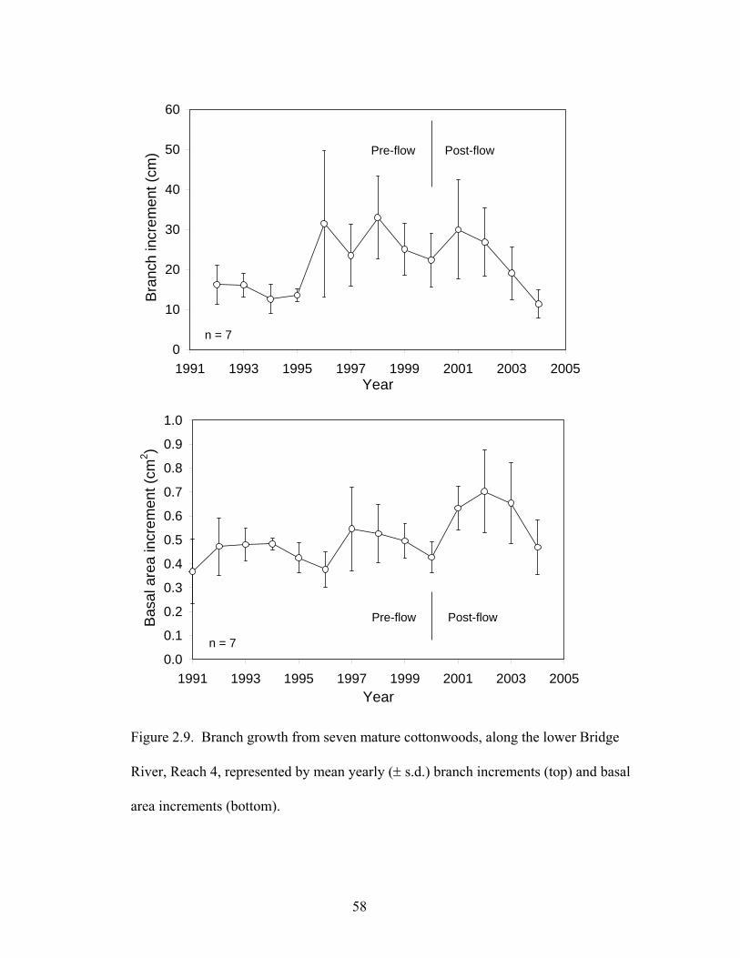
0

10

20

30

40

50

60

1991 1993 1995 1997 1999 2001 2003 2005Year

Bra

nch

incr

emen

t (cm

) Post-flowPre-flow

n = 7

0.0

0.1

0.2

0.3

0.4

0.5

0.6

0.7

0.8

0.9

1.0

1991 1993 1995 1997 1999 2001 2003 2005Year

Bas

al a

rea

incr

emen

t (cm

2 )

Pre-flow Post-flow

n = 7

Figure 2.9. Branch growth from seven mature cottonwoods, along the lower Bridge

River, Reach 4, represented by mean yearly (± s.d.) branch increments (top) and basal

area increments (bottom).

58

2.3.4 Juveniles

To smooth the data and integrate growth over multiple years juvenile tree growth was

analyzed in four year averages (Figure 2.10). The pre-flow group of juveniles

displayed a reduced average growth relative to the post-flow group (Figure 2.10). The

transition group apparently increased through the interval as the trees establishment

date moved towards the year 2000, when the experimental flow commenced. This can

be explained because most of the growth experienced by these later trees would have

been during the flow-release time period, even though their establishment would have

been prior to the flow release, thus potentially increasing their growth (Figure 2.10).

The non-parametric Kruskal-Wallis test and the parametric ANOVA test showed that

the pre-flow, transition and post-flow groups varied significantly (p<0.001) (Table 2.

5, Appendix 6). To determine how the three groups varied we applied Mann-

Whitney non-parametric paired-comparisons. These tests indicated that the pre-flow

and the transition group probably differed (p = 0.055), the pre-flow and the post-flow

groups were highly significantly different from each other (p<0.001). While the post-

flow and the transition groups (p = 0.114, Table 2.6), were not significantly different.

59

Transition

(ab)

y = 0.687x - 1370r2 = 0.485

n.s.

0

1

2

3

4

5

6

7

1990 1992 1994 1996 1998 2000 2002 2004Year of establishment

Rad

ial i

ncre

men

t (m

m)

Pre-flow

(b)

Post-flow

(a)

n = 13 n = 5 n = 12

a

Figure 2.10. Mean radial increments for the first four years of growth of juvenile

cottonwood trees along lower Bridge River Reach 4. Data are displayed in groups of

trees according to year of establishment, either during the pre-flow, transition or post-

flow, time periods. Groupings associated with different letters (a, b) differ

significantly, while the ab group is a combination of both. Mean values are indicated

by dashed lines for the pre-flow and post flow groups. The apparent trend is shown

for the transition group and thus could link the two means.

60

Table 2.5. Kruskal-Wallis test (a non-parametric approach for analysis of

variance), results from three groups of juvenile cottonwood trees along the lower

Bridge River Reach 4 as shown in Figure 2.10.

Kruskal-Wallis Test

Group N

Mean

Rank χ2 df Probability

Pre-flow 13 9 14.0 2 0.001***

Transition 5 16.4

Post-flow 12 22.2

Total 30 *** = P<0.001

61

Table 2.6. Mann-Whitney test (non-parametric paired-comparisons) results for

juvenile cottonwoods separated into pre-flow, transition and post-flow groups along

the lower Bridge River, as shown in Figure 2.10.

Mann-Whitney Test

Comparison n

Mean

rank Z Probability

Pre-flow vs.

Transition

13

+ 5

8.0 vs.

13.4

-

1.

92 0.055 t

Pre-flow vs. Post-

flow

13

+

12

8.0 vs.

18.4

-

3.

54 0.000 ***

Transition vs. Post-

flow

5 +

12

6.0 vs.

10.3

-

1.

58 0.114 n.s.

t = P<0.1; *** = P<0.001; n.s. = not significant

62

The juvenile trees sampled along the lower Bridge River ranged from 3 to 28 years

old with the basal stem diameters ranging from 5 cm to 11 cm (Figure 2.11). These

trees were compared to Yalakom River juvenile trees that also ranged from 5 to 11

cm in trunk diameter. The majority of trees sampled along both rivers are within the

age range of 5 to 13 years old in the comparison of basal area increments vs. years,

displayed in the 10 year comparison (Figure 2.12). Juvenile trees from the lower

Bridge River displayed a greater increase in growth after 2000 compared to the

juvenile trees growing along the Yalakom River (Figure 2.12). We had insufficient

data to determine if the data have a normal distribution. So we used an independent

samples t-test (parametric) and a Mann-Whitney test (non-parametric) to compare the

means of juvenile growth. Both tests display a significant difference in juvenile

growth rates along the lower Bridge River vs. the Yalakom River (Appendix 5).

The trunk diameter of cottonwoods normally increases with increasing age of the tree

which can be seen in the juvenile Yalakom data (Figure 2.13). However, the lower

Bridge River data did not display the same pattern, as data were more scattered with

some trees displaying apparently stagnant growth (Figure 2.13). The Mann-Whitney

test was used to determine if there was a difference between the two groups of data.

The data was ranked and then tested resulting in the data not being significantly

different with an assumptive significance (2 tailed) of 0.164. We also analyzed the

growth patterns of the juvenile cottonwoods data set that was used in (Figure 2.11)

but without the two oldest samples (Figure 2.13).

63

0

2

4

6

8

10

12

1 3 5 7 9 11 13 15 17 19 21 23 25 27Age (Years)

Num

ber o

f juv

enile

sBridge (n=31)

Yalakom (n=26)

Sample range used for comparison

Figure 2.11. Juvenile cottonwoods from the regulated lower Bridge River Reach 4

and the free-flowing Yalakom River: number of individuals versus age.

64

0

1

2

3

4

5

6

7

8

9

10

1996 1998 2000 2002 2004 2006Year

Bas

al a

rea

incr

emen

t (cm

2 )

Bridge (n=16)Yalakom (n=24)

Pre-flow Post-flow

*

*

*

**

Figure 2.12. Average (± s.d.) annual basal area increments (BAI) of juvenile trees

from the lower Bridge River Reach 4 and Yalakom River during pre and post-flow

conditions. *, ** = indicate significance of (p<0.05, p< 0.01 respectively), differences

in basal area increment as detected by t- tests.

65

Yalakom y = 0.372x + 1.480

r2 = 0.16p = 0.01

0

2

4

6

8

10

12

0 2 4 6 8 10 12 14 16 18Age (years)

Dia

met

er (c

m)

Bridge (n=30)Yalakom (n=25)

Figure 2.13. Juvenile cottonwood trees along the lower Bridge River Reach 4 and

Yalakom River, trunk diameter versus age.

66

2.3.5 Saplings

The final age class of cottonwoods sampled along the lower Bridge River was

included as an afterthought due to the inconspicuous nature and size of the saplings.

To determine if experimental flows were affecting the recruitment of sapling-aged

cottonwoods in Reach 4, studies were undertaken in 2005 to initially determine, if

this age class existed in that specific reach. The entire 4 km of Reach 4 was

investigated for saplings with one specific location along Reach 4 providing an

excellent band of saplings, in which sampling was focused (Figure 2.15).

When data collection for this study began in 2003 the saplings that were collected in

2006 would have been barely visible as a distinct riparian tree. It was only once these

saplings had reached their third year, when rapid growth is likely to occur, that they

became readily apparent (Figure 2.15).

Cottonwoods require favorable conditions for recruitment such as barren sites, fine

sediments and slowly declining water levels to survive throughout the growing season

and the first critical year of growth (Rood et al. 2003a). The experimental flow

regime of the lower Bridge River has attempted to mimic a seasonal snow-melt

dominated hydrograph. The receding limbs of these hydrographs exhibit steep, sharp

declines in water stage in the first few years of operations, but become more gradual

in the later years (Figure 2.5).

67

The majority of saplings aged by bud scar counting indicate that they were

established in 2002. The saplings that were aged using ring verification indicate that

the majority of establishment occurred in 2003, corresponding with the gradual flow

decreases (Figure 2.14).

68

Bud scar counted saplings (n = 59)

0

5

10

15

20

25

30

35

200520042003200220012000

Freq

uenc

y of

indi

vidu

als

Ring verified saplings(n = 59)

0

5

10

15

20

25

30

35

200520042003200220012000Year of establishment

Bud scar counted saplings(n = 200)

0

10

20

30

40

50

60

70

80

200520042003200220012000Year of establishment

Freq

uenc

y of

Indi

vidu

als

Figure 2.14. Establishment years of cottonwood saplings that were studied and

harvested from the lower Bridge River Reach 4. Age was determined using annual

bud scar counting done in the field compared to basal cross-section ring counting

done in the lab.

69

Saplings

Juvenile

Mature

Figure 2.15. Lower Bridge River Reach 4, left bank with new band of saplings in the

foreground with juvenile cottonwoods midway up the bank and mature trees higher

up, July 28, 2006, top, December 31, 2006, bottom. The black arrows indicate the

same juvenile tree.

70

2.4 Discussion

The results of this study suggest that specific age classes of black cottonwood trees

growing along the lower Bridge River in south-western British Columbia have

displayed an increase in growth, due to the re-introduction of flow to Reach 4. Since

the summer of 2000 the Bridge River has become a different river than it was

historically. It is no longer the big river it was in the past, but since the summer of

2000 the lower Bridge River has surface flow once again.

Over the past seven years it has been altered, shaped and modified into a much

smaller regulated river with a functioning seasonal hydrograph. The effect that this

seasonal hydrograph has had on the riparian cottonwoods can be seen in the increased

growth of these trees but predominantly in the recruitment of young cottonwoods.

The study investigated three specific age groupings of riparian black cottonwoods

growing throughout the watershed in attempts to determine the effects that surface

flows have on the trees in this river system.

Mature cottonwoods along Reach 4 of the lower Bridge River did not display a

response to the increase in flow. One explanation for this non-response can be

explained by their large physical size which also indicates intricate deep rooting

systems, making it possible for the mature trees to reach and utilize the groundwater

resource (Reily and Johnson 1982). This has also been stated by Stromberg and

Patten (1990), in relation to vegetation that could be reliant on a subsurface or

71

groundwater resource if surface flow is unavailable. Physical size determination

would also explain the potential for groundwater to be unavailable to younger and

smaller trees, thus indicating that surface water would be more readily available,

which suggests that any flow changes in the river would likely affect them.

Although previous studies (Willms et al. 1998) found that branch growth was

hydrologically more responsive to water changes than radial trunk increment growth,

this was not verified amongst the mature trees along the lower Bridge River. The

trunk and branch radial increment growth analysis did not show any significant

response to the 3m3/s discharge of the lower Bridge River.

Juvenile cottonwoods displayed an increase in growth in regards to annual growth.

The location of juveniles was at a lower elevational position on the river bank than

the mature trees. Juvenile cottonwoods grow at an increased rate. To compare sample

populations from along the lower Bridge and Yalakom Rivers, we ensured that all

samples were of the same age and trunk size class. The juvenile trees growing along

the lower Bridge River grew consistently faster or with more vigor than the juveniles

growing along the Yalakom River during the same time period.

When deciphering tree growth during the pre-flow and post-flow time periods, the

lower Bridge River cottonwoods displayed increased growth patterns post-flow

(after) the flow releases in 2000. This confirmed our hypothesis that the increase in

72

surface flow in the lower Bridge River would increase growth among riparian

cottonwoods, but only in a particular age class.

The next discovery of cottonwood growth along the lower Bridge River was a

gratifying realization that regeneration in the form of establishment was taking place

the entire time the study was focused on the mature and juvenile age classes. During

the initial years of data collection in 2003, the lower Bridge River cottonwood

saplings were growing as an invisible population disguised by the tall grasses and

shrubs. It was not until the third year of data collection along the lower Bridge River

that the sapling age class revealed itself as a strong recruitment event that was

significantly correlated with the seasonal re-introduction of flow in the lower Bridge

River.

Saplings were analyzed to determine year of establishment in regards to the increased

flow in Reach 4. The 59 ring-verified saplings displayed a different age structure in

the lab than compared to age measurements taken in the field. By comparing these

two methodologies, we determined that node counting is a reliable way to assess

sapling ages in field conditions whereas ring verification of the samples is more

accurate. The number of similarly aged saplings in this previously dewatered reach

indicates there was a major event that resulted in a large recruitment event.

This initial peak in recruitment is usually followed by a gradual decline in recruitment

year by year, which can be explained by looking at patterns of establishment among

73

cottonwoods that depict a natural decline in numbers of sapling established in years

following a large hydrologic event (Rood et al. 2003a). The effective establishment of

saplings along the lower Bridge River indicates that the seasonal flow pattern of the

Bridge River from 2000 – 2006 has been effective at creating a healthy riparian zone

in which cottonwoods are reproducing.

74

2.5 Conclusion and management implications

In the future, the lower Bridge River should be managed in a way that will enhance

and embrace the connectivity of aquatic and riparian systems without compromising

the functionality of the hydroelectric operations in the Bridge watershed. This study

has shown that it is not necessarily the volume of historic flows that are needed in the

lower Bridge River, but the presence of surface water in conjunction with a seasonal

flow regime.

The riparian zone response has been documented and displays the increased growth

of juveniles and the recruitment of young cottonwoods. These documented increases

in cottonwood growth are the beginning of the cycle of riparian forest succession.

Such growth is further rejuvenating a previously compromised ecosystem. These

findings have led us to view the Bridge River today as a functioning river rather than

a river that has been fully restored.

The Bridge River has essentially been re-sized and re-constructed into a different

river today than the historical pre-dam version. Today the results from the

experimental flows can be regarded as functional flows in that they perform all the

necessary tasks of a river but at a vastly reduced scale. Thus, the Bridge River no

longer has historic discharge levels but does maintain functional flows that uphold the

seasonality of a snowmelt dominated hydrograph, thus reviving Reach 4 of the lower

Bridge River.

75

2.6 Literature cited

Abernethy, B., and I. D. Rutherfurd. 2001. The distribution and strength of riparian

tree roots in relation to riverbank reinforcement. Hydrological Processes. 15: 63-

79.

Annear, T., I.C. Chisholm, H.B. Beecher, A. Locke, P.A. Aarrestad, N. Burkhart, C.

Coomer, C. Estes, J. Hunt, R. Jacobson, G. Jobsis, J. Kauffman, J. Marshal, K.

Mayes, C. Stalnaker, and R. Wentworth. 2002. Instream flows for riverine

resource stewardship. Instream flow council, Cheyenne, Wyoming, USA.

Amlin, N. M. and S. B. Rood. 2003. Drought stress and recovery of riparian

cottonwoods due to water table alteration along Willow Creek, Alberta. Trees.17:

351-358.

Berg, K. J., G. M. Samuelson, C. R. Willms, D. W. Pearce, and S. B. Rood. 2007.

Consistent growth of black cottonwoods despite temperature variation across

elevational ecoregions in the Rocky Mountains. Trees. 21: 161-169.

Braatne, J. H., R. Jamieson, K. M. Gill, and S. B. Rood. 2007. Instream flows and the

decline of riparian cottonwoods along the Yakima River, Washington, USA.

River Research and Applications. 23: 247-267.

76

Bradford, M. J., and P. S. Higgins. 2001. Habitat-, season-, and size-specific variation

in diel activity patterns of juvenile Chinook salmon (Oncorhynchus tshawytscha)

and steelhead trout (Oncorhynchus mykiss). Canadian Journal of Fisheries and

Aquatic. 58: 365-374.

Brayshaw, T. C. 1965. The status of the black cottonwood (Populus trichocarpa

Torrey and A. Gray). The Canadian Field Naturalist. 79: 91-95.

Church, B. N. 1996. Bridge River mining camp geology and mineral deposits.

Energy and Minerals Division, Geological Survey Branch, British Columbia.

Clark, J. 2006. Fisheries Act cases involving BC Hydro operation in the Pacific

Region. Prairie Provinces Water Board (PPWB) Instream Flow Needs Workshop

Report. March 2006, Calgary, Alberta, Canada. 41 pp.

Conlin, K., C. Lamont, and S. MacFarlane. 2000. BC Hydro: Bridge-Coastal Fish and

Wildlife Restoration Program: Strategic Plan, Volume 1 & 2, Ch.10-11.

Dykaar, B. B., and P. J. Jr. Wigington. 2000. Floodplain formation and cottonwood

colonization patterns on the Willamette River, Oregon , USA. Environmental

Management 25: 87-104.

77

Failing, L., G. Horn, and P. S. Higgins. 2004. Using expert judgment and stakeholder

values to evaluate Adaptive Management options. Ecology and Society. 9 (1): 13.

Farrar, J. L. 1995. Trees in Canada. Fitzhenry & Whiteside Ltd. Markham, Ontario

and the Canadian Forest Service Ottawa, Ontario, Canada. pp. 338-339.

Gadd, B. 1995. Handbook of the Canadian Rockies, Second Edition. Corax Press,

Jasper Alberta, Canada. 831 pp.

Gillilan, D. M., and T.C. Brown. 1997. Instream flow protection: seeking a balance in

western water use. Island Press, Washington DC, USA.

Gordon, N. D., T. A. McMahon, B. L. Finlayson, C. J. Gippel, and R. J. Nathan.

2005. Stream Hydrology: An Introduction for Ecologists. Second edition. John

Wiley & Sons Ltd, The Atrium, Southern Gate, Chichester, West Sussex,

England. 429 pp.

Higgins, P. S., and M. J. Bradford. 1996. Evaluation of a large-scale fish salvage to

reduce the impacts of controlled flow reduction in a regulated river. North

American Journal of Fisheries Management 16: 666-673.

78

Hill, E. L., and K. G. Wright. 2000. Harlequin duck breeding distribution and

hydroelectric operations on the Bridge River, British Columbia. Proceedings of a

conference on the biology and management of species at risk, Kamloops BC,

1999. Vol. 1. 490 pp.

Karrenberg, S., P. J. Edwards, J. Kollman. 2002. The life history of Salicaceae living

in the active zone of floodplains. Freshwater Biology 47: 733–748.

Kondolf, G. M. 1997. Hungry water: effects of dams and gravel mining on river

channels. Environmental Management. 21: 533-551.

Lemke, S. L. 2000. Moose winter habitat evaluation and enhancement opportunities

in the Bridge River System. BC Hydro Bridge-Coastal Compensation Program

Report. BC Hydro. 24 pp.

Leopold, L. B. 1994. A View of the River. Harvard University Press, Cambridge,

Massachusetts, USA. 298 pp.

Mahoney, J. M., and S. B. Rood. 1998. Streamflow requirements for cottonwood

seedling recruitment - an integrative model. Wetlands 18: 634-645.

79

McPhail, J. D., and R. Carveth. 1993. Field key to the freshwater fishes of British

Columbia. Resources Inventory Committee, Queens Printer for British Columbia,

Victoria, BC. 239 pp.

Ministry of Environment, Water Stewardship Division. 2007. Dams in BC.

Government of British Columbia. Accessed January 10, 2007.

http://www.env.gov.bc.ca/wsd/public_safety/dam_safety/responsible.html#dams

Naiman, R. J., and H. Décamps. 1997. The ecology of interfaces: riparian zones.

Annual Review of Ecology and Systematics. 28: 621-658

Naiman, R. J., H. Décamps, and M.E. McClain. 2005. Riparia: Ecology,

Conservation, and Management of Streamside Communities. Elsevier Academic

Press, Amsterdam 430 pp.

Nanson, G. C., and H. F. Beach. 1977. Floodplain succession and sedimentation on a

meandering-river floodplain, northeast British Columbia, Canada. Journal of

Biogeography. 4: 229-251.

Parish, R., R. Coupe, and D. Lloyd. 1996. Plants of southern interior British

Columbia. Lone Pine Publishing, Vancouver, B.C. 463 pp.

80

Peterson, R. T., and V.M. Peterson. 1990. A Field Guide to Western Birds. Houghton

Mifflin Company, New York, New York. 432 pp.

Polzin, M. L., and S. B. Rood. 2000. Effects of damming and flow stabilization on

riparian processes and black cottonwoods along the Kootenay River. Rivers. 7:

221-232.

Polzin, M. L., and S. B. Rood. 2006. Effective disturbance: seedling safe sites and

patch recruitment of riparian cottonwoods after a major flood of a mountain river.

Wetlands. 26: 965-980.

Reily, P., and W. Johnson. 1982. The effects of altered hydrologic regime on tree

growth along the Missouri River in North Dakota. Canadian Journal of Botany.

60: 2410-2423.

Rood, S. B., J. M. Mahoney, D. E. Reid, and L. Zilm. 1994. Instream flows and the

decline of riparian cottonwoods along the St. Mary River, Alberta. Canadian

Journal of Botany. 73: 1250-1260.

Rood, S. B., J. H. Braatne, and F. M. R. Hughes. 2003a. Ecophysiology of riparian

cottonwoods: stream flow dependency, water relations and restoration. Tree

Physiology. 23: 1113-1124.

81

Rood, S. B., A. R. Kalischuk, M. L. Polzin, and J. H. Braatne. 2003b. Branch

propagation, not cladoptosis, permits dispersive clonal reproduction of riparian

cottonwoods. Forest Ecology and Management. 186: 227-242.

Ryder, J. 1991. Geomorphological processes associated with an ice-marginal lake at

Bridge Glacier, British Columbia. Geographie Physique et Quaternaire. 45: 35-44.

Scott, M., P. Shafroth, and G. Auble. 1999. Responses of riparian cottonwoods to

alluvial water table declines. Environmental Management. 23: 347-358.

Shafroth, P., J. Friedman, G. Auble, M. Scott, and J. Braatne. 2002. Potential

responses of riparian vegetation to dam removal. BioScience. 52: 703-712

Stromberg, J., and D. Patten. 1990. Riparian vegetation instream flow requirements: a

case study from a diverted stream in the Eastern Sierra Nevada, California, USA.

Environmental Management. 14: 185-194.

Willms, C. R., D. W. Pearce, and S. B. Rood. 2006. Growth of riparian cottonwoods:

a developmental pattern and the influence of geomorphic context. Trees. 20: 210-

218.

82

Willms, J., S. B. Rood, W. Willms, and M. Tyree. 1998. Branch growth of riparian

cottonwoods: a hydrologically sensitive dendrochronological tool. Trees. 12: 215-

223.

Woo, E. 1998. BC Hydro and DFO sign $600,000 agreement resolving fish habitat

issues at Bridge River. Habitat Enforcement Bulletin, Fisheries and Oceans

Canada, Pacific Region. No. 4.

83

Appendix 1

y = 10.4Ln(x) + 11.3r2 = 0.974p<0.001

0

10

20

30

40

50

60

1 10 100Recurrence Interval (Years)

Max

imun

mea

n da

ily d

isch

arge

(Q

max

, m3 /s

) 1999

1990

1991

Yalakom River

Appendix 1. Recurrence analysis for the free-flowing Yalakom River 1983-2005

(Station 08ME025) (Water Survey of Canada, accessed 2007).

84

Appendix 2

Vegetation

western red cedar Thuja plicata

Pacific silver fir Abies amabilis

horsetail Equisetum spp.

Ponderosa pine Pinus ponderosa

Douglas-fir Pseudotsuga menziesii

saskatoon Amelanchier alnifolia

redstem ceanothus Ceanothus sanguineus

black cottonwood Populus trichocarpa

trembling aspen Populus tremuloides

paper birch Betula papyrifera

mountain alder Alnus incana

Sitka willow Salix sitchensis

(Parish et al. 1996)

85

Appendix 3

Birds

Canadian geese Branta canadensis

trumpter swan Cygnus buccinator

common merganser Mergus merganser

harlequin ducks Histrionicus histrioicus

(Peterson 1990, Hill and Wright 2000)

Mammals

bighorn sheep Ovis canadensis

moose Alces alces

grizzly bear Ursus horribilis

black bear Ursus americanus

cougar Puma concolor

mule deer Odocoileus hemionus

(Gadd 1995)

86

Appendix 4

Anadromous fishes

chinook Oncorhynchus tshwytscha

coho salmon Oncorhynchus kisutch

sockeye salmon Oncorhynchus nerka

pink salmon Oncorhynchus gorbuscha

steelhead Oncorhynchus mykiss

Pacific lamprey Lampetra tridentata

Resident fishes rainbow trout Oncorhynchus mykiss

bull trout Salvelinus confluentus

bridgelip suckers Catostomus columbianus

sculpin Cottus spp.

mountain whitefish Prosopium williamsoni

(Higgins and Bradford 1996, McPhail and Carveth 1993)

87

Appendix 5: One-way ANOVA test for Figure 2.10, page 58.

Descriptives

N Mean Std. Dev

Std. Err

95% Confidence Interval for Mean Min Max

Lower Boun

d

Upper Boun

d

1 6 6.06 1.30 0.53 4.70 7.43 3.83 7.15

2 6 8.59 3.95 1.61 4.44 12.7 3.82 15.1

3 6 13.2 4.12 1.68 8.91 17.5 9.84 20.7

Total 18 9.29 4.40 1.04 7.10 11.5 3.82 20.7

ANOVA

Sum of Squares df

Mean Square F Sig.

Between Groups 158 2 79.2 6.94 0.01 Within Groups 171 15 11.4 Total 330 17

88

Appendix 6: Independent samples Test, Mann-Whitney Test, Figure 2.12, p63.

Independent Samples Test

Levene's Test for

Equality of Variances t-test for Equality of Means

F Sig. t df Probability 2003

Equal variances assumed

4.27

0.046 2.21 38 0.03

Equal variances not assumed 2.03 23.3 0.05

2004

Equal variances assumed

15.4

0.000 3.11 38 0.00

Equal variances not assumed 2.64 17.3 0.02

2005

Equal variances assumed

20.0

0.000 3.33 38 0.00

Equal variances not assumed 2.80 16.8 0.01

2006

Equal variances assumed

18.1

0.000 3.09 38 0.00

Equal variances not assumed 2.56 16.0 0.02

Mann-Whitney Test

2003 2004 2005 2006 Mann-Whitney U 124 87 81 75 Z -1.88 -2.90 -3.06 -3.23 Asymp. Sig. (2-tailed) 0.060 0.004 0.002 0.001

89