An Advance Seminar Paper on

Restricted BoltzmannMachines

Written and Submitted by:

Name: Indraneel Pole

Matrikel Nr: 1063525

Course: Computational Intelligence

1

Table of Contents

Introduction......................................................................................................................3

Theoretical Background..................................................................................................5

Structure of RBM...........................................................................................................5

Mathematical Background of RBM…………………………………………………...7

Graphical model….………………………………………………………………….....8

Training RBM…………………………………………………………………………10

Machine learning and training sets…………………………………………………...10

Supervised v/s unsupervised learning………………………………………………...10

Training RBM………………………………………………………………………...10

MATLAB Code………………………………………………………………………14

Application of RBM…………………………………………………………………...18

Using RBM as DBN………………………………………………………………….18

Motion Detection/learning using RBM………………………………………………19

Whisper speech recognition………………………………………………………….20

Phone recognition…………………………………………………………………….21

Advantages of RBM…………………………………………………………………..24

Limitations…………………………………………………………………………….24

List of Scientific Papers………………………………………………………………25

References……………………………………………………………………………..26

2

Introduction

Restricted Boltzmann Machines, or more generally Boltzmann Machines are part of Artificial Neural Networks family, which are used in machine learning process, to train machines in making stochastic decisions on their own.

Restricted Boltzmann Machines abbreviated as RBM, are used as generative models of different types of data, which can learn a probability distribution over a certain set of its inputs. In their conditional form (where a certain condition is imposed upon them), they can be used to model high dimensional temporal sequences such as audio or video streams. Their most important use however is to work as learning modules which can bestacked up to form deep belief networks.[1]

Invention of BM goes long back in 1980s, when it was first conceptualized by Paul Smolensky under the name of Harmonium.I In 1980s, multiple researches were going on surrounding neural networks and training datasets. While Hinton at al. presented the paper named Analyzing co-operative computation in 1983, which were based on Hopfield’s research on neural networks and physical systems (Boltzmann machines are Monte Carlo version of Hopfield networkII), around the same time Smolensky also talked about similar ideas called “Harmony Functions”.[8]

Although Boltzmann machines were theoretically invented in late 1980s, training them was very complex, and impractical back then because of the two important effects.

1. The time to calculate equilibrium statistics grows exponentially with the size of Machine.

2. As every unit was connected to other unit, connections became too complex too quickly.[7]

After the invention of fast learning algorithms by Hinton after year 2000, and the restrictions put on features of Boltzmann machines (Which gave the term Restricted Boltzmann machines) made them quite useful and popular in recent times.

The restricted Boltzmann machines are important in many scientific fields. The conclusions or results of Boltzmann machine are often used as a tool for certain optimization problems which also include difficult combinational problems. An excellent example of such problems is “Travelling Salesman problem”.[1]

I A learning model based on harmony theory

II A form of recurrent artificial neural network invented by John Hopfield in 1982

3

Because of their rich structure, learning of RBM is expected to fit into complex prior distributions. That is the reason why Boltzmann machines are important in solving informational problems that require suitable prior distributions.

This seminar paper is focusing upon the training of Restricted Boltzmann Machines to perform stochastic inferences. It also talks about the advantages and limitations of using RBM in machine learning scenarios, as well as explains briefly about the applications ofRBM in machine learning. Further it emphasizes on the role of RBM in building deep belief networks and feed forward nets. The seminar paper also consists of source code and explanation of an application that is built using MatLab to demonstrate the implementation of restricted Boltzmann machines. This seminar paper is based on extensive research published in the form of scientific papers; references and copies of which are given at the end of the paper.

4

Theoratical Background

When the stochastic processing units together create networks which have bidirectional connections, they form Boltzmann machines. These networks can be interpreted as neural network models. A Boltzmann machine is normally used to learn important aspects of an unknown probability distribution function based on given samples of this distribution function. However, because each stochastic processing unit is connected to all the other processing units, this process of leaning certain aspects of a probability distribution becomes quite lengthy, complex, and most importantly time consuming. To simplify this learning process, some restrictions can be applied on the Boltzmann machines. These restrictions give birth to new set of generative models known as Restricted Boltzmann Machines.[1][2]

A restricted Boltzmann Machine acts as a parameterized generative modelIII in order to represent unknown probability distributions. By parameterized it means that RBM can adjust its parameters in order to make the probability distribution of RBM fit the trainingdataIV as much as possible.

Structure of RBM

A Restricted Boltzmann Machine consists of the two sets of units known as visible and hidden units (so called neurons). This can be modeled as being arrange in two different layers. In a normal Boltzmann Machine, each unit can talk to all the other units; however in RBM intra-layer communication is not possible. That means there is no visible – visible or hidden – hidden communication that can take place in RBM.

A visible layer consists of the units that are directly observed or measured in RBM, i.e. they consists input units for RBM. Hidden units on the other hand as the name suggests are not directly connected to training data, and are there to model dependencies betweencomponents. Hidden units are inferred from visible units. They are non – linear detectors, also known as latent variables. Hidden units are important in learning process because they reduce the dimensionality of data to great extent.[11]

III A model that is randomly generating observable data

IV Set of data to discover potentially predictive relationships

5

Fig.1: Hidden units are denoted by h, while visible units are denoted by v.

To understand this bipartite architectureV of RBM more clearly, let us take an example ofbinary images as a training set for RBM. This training set can be modeled using two-layer network in which random binary pixels are representing visible units, and are connected to stochastic binary feature detectors modeled as hidden units. These connections are weighted using symmetrical weights. Because the state of pixels is observed, they are terms as visible units.[7][13]

V Architecture whose vertices can be divided in two disjoint sets

6

Mathematical background of RBM

To understand this further, a mathematical model with the help of aforementioned example of binary image can be presented.

As stated earlier, for a training set of binary images, stochastic pixels are visible units, while feature detectors for the pixels are hidden units. Connections between hidden and binary units are symmetrically weighted. Here, it has to be noted that being a Restricted Boltzmann Machine, hidden or visible units cannot have intra layer connection, i.e. hidden – hidden(feature detector-feature detector) or visible-visible (pixel-pixel) connections are not possible.

Hidden and visible units together have energy, which can be given by:

E(v,h) = -Σiaivi -Σjbjhj –Σivihjwij

Where v is binary state of visible unit at i, h is binary state of hidden unit at j; a, and b are biases, and w is symmetric weighting factor for connections between two units. The structure itself assigns a probability to each connection vector between hidden and visible units. This probability can be written in a mathematical equation with the help of energy function.

P(v,h) =1/Z*e-E(v,h)

Here Z is the summation over all the possible connections between two layers.

Z =Σv,he-E(v,h)

The probability assigned to a visible unit can be calculated by summing over all the possible hidden units, and vice versa. [2][5]

p(v) =1/ZΣhe-E(v,h)

According to Geoffrey Hinton (inventor of Boltzmann Machines) – “The probability that the network assigns to a training image can be raised by adjusting the weights and biases to lower the energy of that image and to raise the energy of other images, especially those that have low energies and therefore make a big contribution to the partition function. The derivative of the log probability of a training vector with respect to a weight is surprisingly simple.”[2]

∂ log p(v)/∂wij= <hvihj>data − <hvihj>model

Here brackets represent the expectations under the distribution. These also denote that:

7

∆wij = ε(<vihj>data - <vihj>recon)

Usually getting unbiased sample of <vihj> data, however, the restriction put on Boltzmann Machine in the form of RBM comes to rescue in this case. Because hidden units in RBM do not have any hidden connections in between them, it is very easy to obtain this unbiased sample of data.

Getting unbiased sample of model data on the other hand is quite difficult. It can be achieved by starting randomly at any of the visible units and then performing alternatingGibbs sampling for a long period of time. We will talk more about these learning strategies later while discussing Training Algorithms for RBM.

Graphical model

Any complex computational problem can be solved more efficiently if algorithms manage to exploit the graph structures for their use. Graphical models are quite useful while plotting and calculating probability distributions. Graphical models denote conditional dependence and independence properties between random variables on a graph structures. Graphical models are commonly used in machine learning.

Restricted Boltzmann Machines are special types of Markov Random Fields also knownas undirected graphical model. Undirected graph model is a structured set of data with finite set of nodes V and a set of undirected edges E. An edge can be constructed out of two nodes from V. The tupleVI can be denoted as:

G = (E, V)

On a stripped down level, Markov Random Fields are type of undirected graphs whose edges have dependencies. Random variables X = (Xv)veE, where v is a node in undirected graph, are called Markov Random Field, if the joint probability distribution fulfills the Markov property.[1][17]

VI Database

8

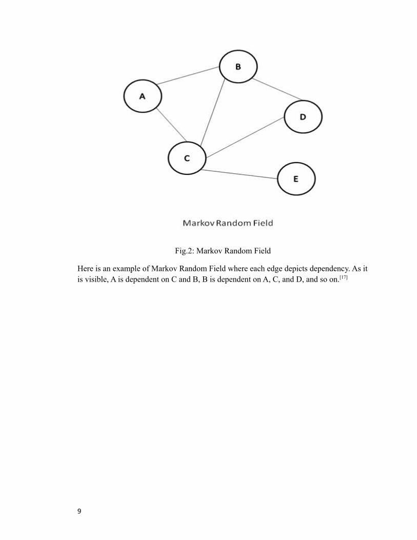
Fig.2: Markov Random Field

Here is an example of Markov Random Field where each edge depicts dependency. As itis visible, A is dependent on C and B, B is dependent on A, C, and D, and so on.[17]

9

Training RBM

Machine Learning and Training sets

According to peer reviewed scientific journal Machine Learning “Machine learning is a scientific discipline that explores the construction and study of algorithms that can learn from data. Such algorithms operate by building a model based on inputs and using that to make predictions or decisions, rather than following only explicitly programmed instructions.”

Machine learning enables machines to take so called “decisions” on their own regarding certain situation. A large part of machine learning is dependent upon the training algorithms and training data that helps machines in “learning”.

Supervised v/s unsupervised learning

Supervised learning is a way of training machines, where labelsVII are provided to machine with predefined inputs and outputs. The machine is supposed to learn the mapping between input and output in general so that it can assign the same mapping to the future inputs that it gets.

On the other hand, in unsupervised learning, no labels are given to the learning algorithm, and the algorithm or machine has the main task of learning the pattern in the structure of the data.

Training RBM

As we already know, a BM is a parameterized model which represents a Gaussian probability distribution. This feature can be used to learn important aspects of an unknown target based on samples from this particular distribution. RBM is basically “trained” by calculating or more generally put “understanding” the connections betweenhidden and visible units using labeled or training data. These connections are denoted asweights. These weights later can be applied to understand the relation for unknown data.To put this in mathematical terminology training a RBM means adjusting the parameters

VII Used in supervised learning where each training set contains pair of given input and desired output sequence

10

of the RBM so that the probability distribution of RBM fits the training data as much as possible.[2]

Fig.3: Parameter Fitting

This is a visual representation of parameter fitting. The training data here is handwritten digits which RBM then models for the distribution.

Fig.4: Generation

After the learning phase is over, the trained RBM then can be used to generate different samples (as shown in the picture above) from the learnt distribution. RBM then providesthe closed form representation of the distribution underlying the training data. RBM can also be trained as classifiers.

11

As we discussed earlier in the mathematical background of RBM, the probability of the network that is assigned to the training data can be increased by adjusting the weights (Wij) and Biases (Ai and Bj) to lower the energy of that particular training set and increase the energy of other sets. Then the derivation of logistic functionVIII with respect to Wij is very simple to put.

∂ log p(v)/∂wij= <hvihj>data − <hvihj>model

P(hj = 1 | v) = σ(bj +Σiviwij)

Where σ(x) is the logistic sigmoid function 1/(1 + exp(−x)). ViHj then is an unbiased sample.

P(vi = 1 | h) = σ(ai +Σjhjwij)

Getting an unbiased sample of <vihj>model on the other hand is quite difficult. To take the unbiased sample of it, we can use the Gibbs SamplingIX method which is described as below.

1. Start with updating any random state of the visible units.

2. Update all the hidden units in parallel using

P(hj = 1 | v) = σ(bj +Σiviwij)

3. Update or Reconstruct all the visible units in parallel using

P(vi = 1 | h) = σ(ai +Σjhjwij)

4. Repeat this process for all the training data.[2][10]

The whole process of training RBM this way is called Contrastive Divergence. Geoffrey Hinton in his paper of training RBM has explained a much faster learning procedure. It differs at the reconstruction phase, where “reconstruction” is produced by setting each visible unit to 1 with a given probability. The change in the weight can thenbe given by:

VIII Log of probability of training vector: log P(V)

IX Markov Chain Monte Carlo (MCMC) algorithm for obtaining a sequence of observations which are approximated from a specified multivariate probability distribution; Used when direct sampling is difficult

12

∆wij = ε(<vihj>data - <vihj>recon)

It has been said that RBM can typically learn better models if more steps of alternating Gibbs sampling are used before negative statistics (the second term in learning rule).

In this seminar paper, we assume that the training data and hidden units are binary and thus, the hidden units should have stochastic binary states.

The learning method of RBM “Contrastive Divergence” can be understood better with an example, which has been also implemented in MATLAB within the scope of this seminar paper. In this example, we have taken six visible states, which denote 6 different movies. The training data that is provided is based on whether a particular user likes this certain movie or not. Each visible unit has binary state, 1 or 0 where 1 denotes to like and 0 denotes to dislike.[10]

The construction has two hidden units where they represent the genre of the movie. Thegoal of this example is to build a connection between the movie and the genre. That is the RBM should predict based on user’s choice of movie that which kind of movies userlike.

To train the RBM for this example, we will follow below steps.

1. First, take a training data set, which is set of six movie preferences. Set the statesof the visible units to the training data.

2. To update the states of the hidden units, we use the logistic activation given above by σ(x)=1/(1+exp(−x))

3. For the jth hidden unit, compute the activation energy using the given function

aj=∑iwijxi

4. Set visible unit’s value to 1 with probability σ(aj) and to 0 with 1- σ(aj).

5. Compute positive statistics for edge (eij) = xi\*xj (This is the measure for the pairs, whether both units in a pair are on or not.)

6. Reconstruct the visible units using similar technique. For each visible unit, compute the activation energy ai and update the state. (This does not necessarily mean that reconstruction will match the original preference.)

7. Now update hidden units again, and compute (eij) = xi\*xj which is negative statistics for each edge.

13

8. Update the weight of each connection.

9. Repeat for all training examples.

This process is continued for maximum number of epochsX or till when the error between training set and its reconstruction falls below a specific threshold.

When hidden units are being driven by data, it is suggested to use stochastic binary states. When they are driven by reconstructions, it is suggested to use probabilities without sampling.

It is also useful to divide the training set in batches. This is more efficient way of updating weights after estimating the gradient on the mini batches of training data. This is helpful in the programs such as MATLAB as it allows matrix – matrix multiplication. [2][10][12]

X Iterations

14

Here is the snippet of MATLAB code for training RBM.

Fig5: MatLab code for training RBM

First we load the training data. There are two sets of databases that we are using. One is for the simple example of learning weights for movies and its genre. There are six visible units and two hidden units. The maximum epochs for this example are 5000.

First we fit the RBM, and learn the weights for connection.

15

Fig6: Using CD algorithm

We calculate positive and negative edges for all the epochs using logistic functions. Then we update the weights as shown below:

Fig7: Updating weights

On the other hand, RBM predict function is predicting the errors using the label data. The weights of the two hidden units given the training data for six units in a matrix, is given below. These weights denote that for which kind of movie, which genre will be turned on. For example, there is high probability that movie number 4 belongs to genre number 1 based on the weights calculated.

Fig8: Weights between 6 visible and 2 hidden units with classification error

16

The same algorithm is also applied to set of images where there are 5000 training sets each with 784 pixels each. Each pixel (visible unit) has a probability of value assigned to it between 0 and 1. There are 100 hidden units which are nothing but feature detectors. Each hidden unit is assigned weight based on the visible unit’s connection with it. These weights can be seen below:

Fig9: Values of weights between 784 visible and 100 hidden units

These weights with respect to hidden units can be visualized as shown below. Each block in the image, denotes a hidden unit. There are total 100 blocks for 100 hidden units. Each hidden unit consist weights from each visible unit (pixel) and denotes which visible unit turns this hidden unit on.

17

Fig10: Weights denoted by 100 Hidden units

18

Applications of Restricted Boltzmann Machine

Although Restricted Boltzmann machines can normally be used in dimensionality reduction, classification, collaborative filtering, features learning, and topic modeling, RBM came to prominence for their use in Deep Belief Nets (DBN).

Using RBMs in DBN

Deep belief nets as general theory in literature suggests are nothing but RBM stacked upon each other. However, in accurate terminology, DBN are NON FEED FORWARD NETWORKSXI. They have first two layers as RBM, and next layers are sigmoid BN.

Stacking up RBM can also be for prioritizing a feed forward network, which essentially is not a DBN.

Fig11: DBN as stacked up RBM consisting of visible and hidden layers (units)

XI Feed forward networks are neural networks where connection between the units do not form a directed cycle

19

20

Training DBN is also very similar to training RBM. This could be achieved as follows.

1. Provide training data to visible layer as it is done in RBM.

2. Let’s call this training data X.

3. Update the first hidden layer from this X, by calculating weights W.

4. Reconstruct the data, using Hidden Layer and calculate X’.

5. Repeat the same step for next pair of layer.

6. Do this for all the payer of layer until top two layers.

It can also be said that DBN is just the extension of RBM, or RBM is single pair DBN.[2]

[12][18]

Apart from building DBN, there are multiple other applications of RBM. Modeling data is one important application among them.

Motion Detection/Learning using RBM

Restricted Boltzmann Machines can be used to learn the motion difference by using differencing frames with the identical input. Human action recognition has multiple applications from surveillance and retrieval systems to traffic management and many other fields. Although it has been considered to be a great research field in image processing and vision research, due to multiple challenges such as background distinction, camera motion, and occlusion, it is still in a development phase.

Usually, any action recognition system models videos as collection of visual frames. These frames can be estimated using feature detectors. To do this, the most efficient method used is usually to build code-words from each frame of the image and to extract the features out of it. It is also possible to combine shape and motion descriptors to generate visual words and represent an action as a sequence of prototypes. To define the difference between two video frames, we usually subtract one frame from another, which preserves the changes (positive and negative both). This creates a simple saliency mapXII for an action.

The subtraction function is able to remove common shapes and background images which are usually not relevant in learning motion difference in any video frame. This also highlights the movement patterns in frame. This leaves us to learn shallow features

XII The Saliency Map is a topographically arranged map that represents visual state of prominence of a corresponding visual scene

21

in order to recognize motion difference. This can be learnt with relatively ease using RBM. Gaussian RBM have been used to learn the action from saliency maps of differentmotion images.[6]

Fig.12: Video frames in top image, while motion detection with reconstruction in thebottom image.

Using RBM, approximation of joint probability distribution of motion difference can represent relation between two images. These approximations lead to learning of shallow features, which can be transformed into learning of high features by stacking upmany such RBM and building a Deep Belief Net from it. It has been speculated that use of DBN can improve the results to much extent.

Motion difference using RBM and Naïve BayesXIII can give accurate recognition rate up to 98.81% for Weizmann datasets.[6][9]

Whisper Speech Recognition

Using RBM as standard conversion model between whisper and speech spectral envelop, it is possible to recognize whisper. While whispering vocal chords do not vibrate, thus the lack of pitch leads to low energy, and an inherent noise like spectral distribution which reduces intelligence of voice. Conversion of whisper to speech is a complex and not so accurate process as it still consist obviously artificial mufflesXIV and suffers from an unnatural patterns of stress and intonations.

However, recent studies have showed the possibility of building a statistical conversion model between whisper and speech spectrum. This also improves accuracy of the estimated pitch. Both objective and subjective evaluations show that this new method improves the quality of whisper.

XIII Type of simple probabilistic classifier

XIV Cover

22

Gaussian Mixer Model (GMM) based voice conversion methods are benefitted more from use of multiple RBMs. The voiced (V) subspace is used to train RBM on spectral envelop features. This models the joint spectral density between whispers and time-aligned speech.[3]

The reconstruction is started with frame to frame Voice/Whisper (V/UV) from input whispers. The spectral envelop packages are obtained from RBM and maximum output probability parameter generation (MOPPG) algorithm.

Fig.13: The top image is spectrogram of Whisper while bottom one is of reconstructedenvelops.

Phone Recognition

Using conventional RBMs instead of hidden Markov models has shown tremendous change in acoustic modeling. Acoustic modeling has been dependent upon Hidden Markov Models (HMM) since long time. The limitations of HMM is their unrealistic independence assumptions and the very limited representational capacity of their hiddenstates. RBMs have been proved to be quite effective while modeling motion difference as stated before, and it is stated that this can also extend to more powerful generative models such as acoustic modeling. A variant of RBM called Conditional RBM (CRBM) can be used to model spectral variations in each phone of voice. In CRBM models vectors of sequential data by considering the visible variables in previous time steps as additional, conditioning inputs.

23

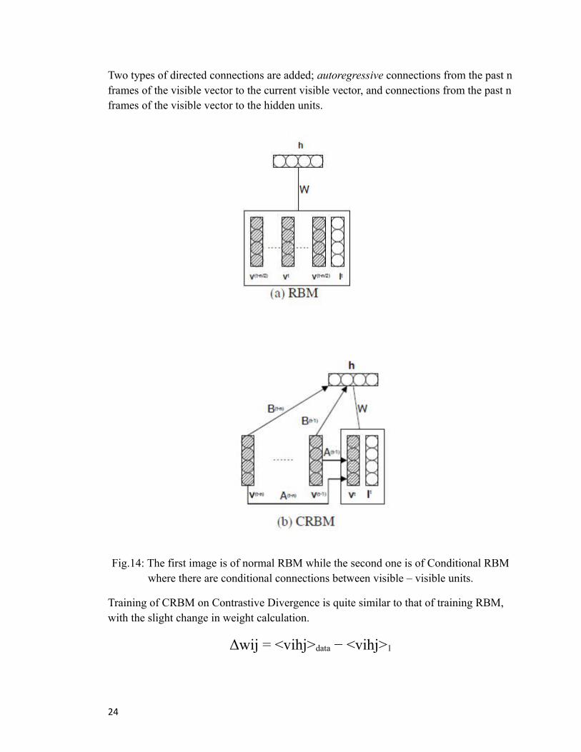
Two types of directed connections are added; autoregressive connections from the past nframes of the visible vector to the current visible vector, and connections from the past nframes of the visible vector to the hidden units.

Fig.14: The first image is of normal RBM while the second one is of Conditional RBMwhere there are conditional connections between visible – visible units.

Training of CRBM on Contrastive Divergence is quite similar to that of training RBM, with the slight change in weight calculation.

Δwij = <vihj>data − <vihj>1

24

Where 1 represents the expectation with respect to the distribution of samples from running a Gibbs sampler initialize the data for one full step.[4]

Update rule for directed connections is also different where for autoregressive visible - visible link it is

ΔA(t−q)ij = v(t−q)

i (<vtj>data − <vt

j>1)

Where A(t−q)ij is the weight from unit i at time (t − q) to unit j.

For the visible-hidden directed links it is

ΔB(t−q)ij = v(t−q)

i (<htj>data −<ht

j>1)

25

Advantages of restricted Boltzmann machine

Expressive enough to encode any distribution while being computationally

efficient

Unlike Hopfield Nets, can encode high-order correlations because of use of

Hidden units

Fast algorithms can be applied because of restrictions put on connections

between hidden-hidden and visible-visible units

Better than auto-encoder in ignoring random noise in the training datasets

Can be stacked up to create DBN, which provide better computational power

The activities of hidden units of one layer can be treated as training data for

higher levels in multiple RBM architecture. This makes overall generative model

quite better[13][14][15]

Limitations of RBM

Cannot efficiently estimate the probability P[x|W]. In simple words estimating the partition function to the same resolution is hard. In fact even approximating it is very difficult and we can only achieve crude approximation.[1][2]

26

List of Scientific Papers

1. Fischer, Asja, Igel, Christian: “Introduction to Restricted Boltzmann Machine”, CIARP 2012, LNCS 7441, pp. 14–36, 2012

2. Li, Jing-jie, McLoughlin, Ian, V., Dai, Li-Rong, Ling, Zhen-hua: “Whisper-to-speech conversion using restricted Boltzmann machine arrays”, IEEE Electronic Letters, 2014 50, (24), pp. 1781-1782

3. Mohamed, Abdel-rahman, Hinton, Geoffrey: “PHONE RECOGNITION USINGRESTRICTED BOLTZMANN MACHINES”, IEEE, 2010, pp. 4354-4357

4. Liu, Jian-Wei, Chi, Guang-Hui, Luo, Xiong-Lin: “Contrastive Divergence Learning for the Restricted Boltzmann Machine”, IEEE, 2013, pp. 18-22

5. Tran, Son, N., Benetos, Emmanouil, Garcez, Artur, d’Avila: “Learning Motion-Difference Features using Gaussian Restricted Boltzmann Machines for EfficientHuman Action Recognition”, IEEE, 2014, pp. 2123-2129

6.

27

References

1. 1. Fischer, Asja, Igel, Christian: “Introduction to Restricted Boltzmann Machine”, CIARP 2012, LNCS 7441, pp. 14–36, 2012

2. Hinton Geoffrey: “A Practical Guide to Training Restricted Boltzmann MachinesVersion 1”, 2010, pp. 1-9

3. Li, Jing-jie, McLoughlin, Ian, V., Dai, Li-Rong, Ling, Zhen-hua: “Whisper-to-speech conversion using restricted Boltzmann machine arrays”, IEEE Electronic Letters, 2014 50, (24), pp. 1781-1782

4. Mohamed, Abdel-rahman, Hinton, Geoffrey: “PHONE RECOGNITION USINGRESTRICTED BOLTZMANN MACHINES”, IEEE, 2010, pp. 4354-4357

5. Liu, Jian-Wei, Chi, Guang-Hui, Luo, Xiong-Lin: “Contrastive Divergence Learning for the Restricted Boltzmann Machine”, IEEE, 2013, pp. 18-22

6. Tran, Son, N., Benetos, Emmanouil, Garcez, Artur, d’Avila: “Learning Motion-Difference Features using Gaussian Restricted Boltzmann Machines for EfficientHuman Action Recognition”, IEEE, 2014, pp. 2123-2129

7. http://en.wikipedia.org/wiki/Restricted_Boltzmann_machine

8. Smolensky, P.: “Information Processing in Dynamic Systems: Foundation of Harmony Theory”, 1986, pp. 194-202

9. Gorelick, Lena, Blank, Moshe, Shechtman, Eli, Irani, Michal, Basri, Michal: “Actions as Space-Time shapes”, IEEE - ICCV, 2005, 29, (12), 2247-2253

10. Chen, Edwin: “Introduction to Restricted Boltzmann Machines”, 2011

11. Cueto, Mar´ıa, Ang´elica, Morton, Jason, Sturmfels, Bernd: “Geometry of the Restricted Boltzmann Machine”, 2009, pp.1-18

12. Roux, N., Le, Bengio, Y: “Representational power of restricted Boltzmann machines and deep belief networks Neural Computation”, 2008, pp.1631–1649

13. https://www.youtube.com/watch?v=fJjkHAuW0Yk

14. http://www.cs.toronto.edu/~hinton/

15. http://learning.cs.toronto.edu/

28

16. http://learning.cs.toronto.edu/publications

17. http://en.wikipedia.org/wiki/Markov_random_field

18. http://deeplearning.net/tutorial/DBN.html

29