1

(1)

(2)

(3)

(4)

(5)

Restricted Least Squares, Hypothesis Testing, and Prediction in the Classical Linear RegressionModel

A. Introduction and assumptions

The classical linear regression model can be written as

or

twhere x N is the tth row of the matrix X or simply as

twhere it is implicit that x is a row vector containing the regressors for the tth time period. The classicalassumptions on the model can be summarized as

Assumption V as written implies II and III. With normally distributed disturbances, the joint density(and therefore likelihood function) of y is

The natural log of the likelihood function is given by

2

(6)

(7)

(8)

(9)

Maximum likelihood estimators are obtained by setting the derivatives of (6) equal to zero and solvingthe resulting k+1 equations for the k $’s and F . These first order conditions for the M.L estimators are2

Solving we obtain

The ordinary least squares estimator is obtained be minimizing the sum of squared errors which isdefined by

The necessary condition for to be a minimum is that

3

(10)

(11)

(12)

(13)

(14)

This gives the normal equations which can then be solved to obtain the least squares estimator

The maximum likelihood estimator of is the same as the least squares estimator.

B. Restricted least squares

1. Linear restrictions on $

Consider a set of m linear constraints on the coefficients denoted by

Restricted least squares estimation or restricted maximum likelihood estimation consists ofminimizing the objective function in (9) or maximizing the objective function in (6) subject to theconstraint in (12).

2. Constrained maximum likelihood estimates

Given that there is no constraint on F , we can differentiate equation 6 with respect to F to get an2 2

estimator of F as a function of the restricted estimator of $. Doing so we obtain’2

where $ is the constrained maximum likelihood estimator. Now substitute this estimator for Fc 2

back into the log likelihood equation (6) and simplify to obtain

4

(15)

(16)

(17)

(18)

(19)

(20)

Note that the concentrated likelihood function (as opposed to the concentrated log likelihoodfunction) is given by

The maximization problem defining the restricted estimator can then be stated as

Clearly we maximize this likelihood function by minimizing the sum of squared errors (y - X$ )N(y -c

X$ ). To maximize this subject to the constraint we form the Lagrangian function where 8N is an mc

× 1 vector of Lagrangian multipliers

Differentiation with respect to $ N and 8 yields the conditionsc

Now multiply the first equation in (18) by R(XNX) to obtain-1

Now solve this equation for 8 substituting as appropriate

The last step follows because R$ = r. Now substitute this back into the first equation in (18) toc

obtain

5

(21)

(22)

(23)

(24)

(25)

With normally distributed errors in the model, the maximum likelihood and least squares estimatesof the constrained model are the same.

We can rearrange (21) in the following useful fashion

Now multiply both sides of (22) by to obtain

We can rearrange equation 21 in another useful fashion by multiplying both sides by X and thensubtracting both sides from y. Doing so we obtain

where u is the estimated residual from the constrained regression. Consider also uNu which is thesum of squared errors from the constrained regression.

where e is the estimated residual vector from the unconstrained model. Now remember that inordinary least squares XNe = 0 as can be seen by rewriting equation 10 as follows

6

(26)

(27)

(28)

(29)

(30)

Using this information in equation 25 we obtain

Thus the difference in the sum of squared errors in the constrained and unconstrained models can

be written as a quadratic form in the difference between and r where is theunconstrained ordinary least squares estimate.

Equation 21 can be rearranged in yet another fashion that will be useful in finding the variance of theconstrained estimator. First write the ordinary least square estimator as a function of $ and g asfollows

Then substitute this expression for in equation 21 as follows

Now define the matrix M as followsc

We can then write $ - $ as c

7

(31)

(32)

(33)

(34)

3. Statistical properties of the restricted least squares estimates

a. expected value of $c

b. variance of $c

The matrix M is not symmetric, but it is idempotent as can be seen by multiplying it by itself.c

Now consider the expression for the variance of $ We can write it out and simplify to obtainc.

8

(35)

(36)

(37)

(38)

We can also write this is another useful form

The variance of the restricted least squares estimator is thus the variance of the ordinary least squaresestimator minus a positive semi-definite matrix, implying that the restricted least squares estimatorhas a lower variance that the OLS estimator.

4. Testing the restrictions on the model using estimated residuals

We showed previously (equation 109 in the section on statistical inference) that

Consider the numerator in equation 37. It can be written in terms of the residuals from therestricted and unrestricted models using equation 27

Denoting the sum of squared residuals from a particular model by SSE($) we obtain

9

(39)

(40)

Rather than performing the hypothesis test by inverting the matrix [R(XNX) RN] and then pre and-1

post multiplying by , we simply run two different regressions and compute the F statistic from the constrained and unconstrained residuals.

The form of the test statistic in equation 39 is referred to as a test based on the change in theobjective function. A number of tests fall in this category. The idea is to compare the sum ofsquares in the constrained and unconstrained models. If the restriction causes SSE to besignificantly larger than otherwise, this is evidence that the data to not satisfy the restriction and wereject the hypothesis that the restriction holds. The general procedure for such tests is to run tworegressions as follows.

1) Estimate the regression model without imposing any constraints on the vector $. Let theassociated sum of squared errors (SSE) and degrees of freedom be denoted by SSE and (n - k),respectively.

2) Estimate the same regression model where the $ is constrained as specified by the

hypothesis. Let the associated sum of squared errors (SSE) and degrees of freedom be denoted

by SSE($ ) and (n - k) , respectively.c c

3) Perform test using the following statistic

where m = (n-k) - (n-k) is the number of independent restrictions imposed on $ by thec

o 2 3 4hypothesis. For example, if the hypothesis was H : $ + $ =4, $ = 0, then the numeratordegrees of freedom (q) is equal to 2. If the hypothesis is valid, then SSE($ ) and (SSE) shouldc

not be significantly different from each other. Thus, we reject the constraint if the F value islarge. Two useful references on this type of test are Chow and Fisher.

5. Testing the restrictions on the model using a likelihood ratio (LR) test

a. idea and definition

The likelihood ratio (LR) test is a common method of statistical inference in classical statistics. The LR test statistic reflects the compatibility between a sample of data and the null hypothesisthrough a comparison of the constrained and unconstrained likelihood functions. It is based ondetermining whether there as been a significant reduction in the value of the likelihood (or log-likelihood) value as a result of imposing the hypothesized constraints on the parameters 2 in the

1 2 nestimation process. Formally let the random sample (X , X , . . . , X ) have the joint probability1 2 n 1 2 ndensity function f(x , x , . . . , x ; 2) and the associated likelihood function L(2; x , x , . . . , x ).

The generalized likelihood ratio (GLR) is defined as

10

(41)

(42)

(43)

(44)

(45)

where sup denotes the supremum of the function over the set of parameters satisfying the null0 ahypothesis (H ), or the set of parameters that would satisfy either the null or alternative (H )

o ahypothesis. A generalized likelihood ratio test for testing H against the alternative H is givenby the following test rule:

where c is the critical value from a yet to be determined distribution. For an " test the constantc is chosen to satisfy

where B(2) is the power function of the statistical test.

We use the term “generalized” likelihood ratio as compared to likelihood ratio to indicate thatthe two likelihood functions in the ratio are “optimized” with respect to 2 over the two differentdomains. The literature often refers to this as a likelihood ratio test without the modifiergeneralized and we will often follow that convention.

b. likelihood ratio test for the classical normal linear regression model

Consider the null hypothesis in the classical normal linear regression model R$ = r. Thelikelihood function evaluated at the restricted least squares estimates from equation 15 is

In an analogous manner we can write the likelihood function evaluated at the OLS estimates as

The generalized likelihood ratio statistic is then

11

(46)

(47)

(48)

(49)

We reject the null hypothesis for small values of 8 or small values of the right hand side ofequation 46. The difficulty is that we not know the distribution of the right hand side ofequation 46. Note that we can write it in terms of estimated residuals as

This can then be written as

So we reject the null hypothesis that R$ = r if

12

(50)

(51)

(52)

(53)

Now subtract from both sides of equation 49 and simplify

Now multiply by to obtain

We reject the null hypothesis if the value in equation 51 is greater than some arbitrary value

.

The question is then finding the distribution of the test statistic in equation 51. We can alsowrite the test statistic as

We have already shown that the numerator in equation 52 is the same as the numerator inequations 37-39. Therefore this statistic is equivalent to the those statistics and is distributed asan F. Specifically,

Therefore the likelihood ratio test and the F test for a set of linear restrictions R$ = r in theclassical normal linear regression model are equivalent.

13

(54)

(55)

(56)

(57)

(58)

c. asymptotic distribution of the likelihood ratio statistic

We show in section on non-linear estimation that

where R is the value of the log-likelihood function for the model estimated subject to the nullc

hypothesis, R is the value of the log-likelihood function for the unconstrained model, and thereare m restrictions on the parameters in the form R(2) = r.

6. Some examples

a. two linear constraints

Consider the unconstrained model

o 2 3with the usual assumptions. Consider the null hypothesis H : $ = $ = 0 which consists oftwo restrictions on the coefficients. We can test this hypothesis by running two regressions andthen forming the test statistic.

1) Estimate

and obtain SSE = (n - 4)s where s is the estimated variance from the unrestricted2 2

model.

2) Estimate

and obtain SSE = (n - 2)s where s is the estimated variance from the unrestrictedc 2 2

model.

3) Construct the test statistic

14

(59)

(60)

(61)

(62)

b. equality of coefficients in two separate regressions (possibly different time periods)

We sometimes want to test the equality of the full set of regression coefficients in tworegressions. Consider the two models below

oWe may want to test the hypothesis H : $ = $ where there are k coefficients and thus k1 2

restrictions. Rewrite the model in stacked form as

1 2and estimate as usual to obtain SSE (no restriction). Note that (n - k) = n + n - 2k. Thenimpose the restriction (hypothesis that $ = $ = $) by writing the model in equation 60 as1 2

Estimate equation 61 using least squares to obtain the constrained sum of squared errors SSEc

1 2with degrees of freedom (n - k) = n + n - k. Then construct the test statisticsc

15

(63)

(64)

(65)

C. Forecasting

1. introduction

Let

t t t1 tkdenote the stochastic relationship between the variable y and the vector of variables x = (x ,..., x ). $ represents a vector of parameters. Forecasts are generally made by estimating the vector of

tparameters , determining the appropriate vector x (sometimes forecasted by )and then

evaluating

The forecast error is given by

There are at least four factors which contribute to forecast error.

a. incorrect functional form

16

(66)

(67)

(68)

tb. the existence of the random disturbance g

tEven if the "appropriate" value of x were known with certainty and the parameters $ weretknown, the forecast error would not be zero because of the presence of g . The forecast error is

given by

tConfidence intervals for y would be obtained from

We can see this graphically as

c. uncertainty about $

0 0Consider a set of n observations not included in the original sample of n observations. Let X0 0denote the n observations on the regressors and y the observations on y. The relevant model

for this out of sample forecast is

0 0where E(g ) = 0 and and g is independent of g from the sample period.

17

(69)

(70)

(71)

(72)

(73)

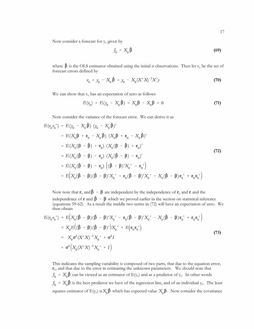
0Now consider a forecast for y given by

0where is the OLS estimator obtained using the initial n observations. Then let v be the set offorecast errors defined by

0We can show that v has an expectation of zero as follows

Now consider the variance of the forecast error. We can derive it as

0 0Now note that g and are independent by the independence of g and g and the

independence of g and which we proved earlier in the section on statistical inference(equations 59-62). As a result the middle two terms in (72) will have an expectation of zero. Wethen obtain

This indicates the sampling variability is composed of two parts, that due to the equation error,0g , and that due to the error in estimating the unknown parameters. We should note that

0 0 can be viewed as an estimator of E(y ) and as a predictor of y . In other words

0 is the best predictor we have of the regression line, and of an individual y . The least

0squares estimator of E(y ) is which has expected value . Now consider the covariance

18

(74)

(75)

(76)

(77)

(78)

(79)

(80)

matrix for the random vector . To simplify the derivation write it as

Then we can compute this covariance as

This is less than the covariance in equation 73 by the variance of the equation error F I. Now2

0 0 0 0consider the case where n = 1 and we are forecasting a given y for a given x , where x N is a row0 0vector. Then the predicted value of y for a given value of x is given by

The prediction error is given by

The variance of the prediction error is given by

0 0The variance of E(y |x ) is

0 0 0Based on these variances we can consider confidence intervals for y and E(y |x ) where we0 0estimate F with s . The confidence interval for E(y |x )is2 2

0where is the square root of the variance in equation 78. The confidence interval for y is given

by

where is the square root of the variance in equation 77. Graphically the confidence bounds in

0 opredicting an individual y are wider than in predicting the expected value of y .

19

d. uncertainty about X. In many situations the value of the independent variable also needs to betpredicted along with the value of y. A "poor" estimate of x will likely result in a poor forecast

for y.

e. predictive tests

One way to consider the accuracy of a model is to estimate it using only part of the data. Thenuse the remaining observations as a test of the model.

11) Compute using observations 1 to n .

12) Compute using the observations on the x's from n to n.

3) Compare the predicted values of y with the actual ones from the sample for1observations n to n.

20

Literature Cited

Chow, G. C., "Tests of Equality Between Subsets of Coefficients in Two Linear Regressions," Econometrica,28(1960), 591-605.

Fisher, F. M., "Tests of Equality Between Sets of Coefficients in Two Linear Regressions: An ExpositoryNote," Econometrica, 38(1970), 361-66.

21

(81)

That equation 38 is distributed as an F random variable can also be seen by remembering that an F isthe ratio of two chi-square random variable, each divided by its degrees of freedom. We have

previously shown (equation 177 in the section on Statistical Inference) that is distributed as

a P (n-k) random variable. Note that the vector is distributed normally with a mean of zero. 2

Its variance is given by