RESTRUCTURING VS. BANKRUPTCY∗

Jason Roderick Donaldson† Edward R. Morrison‡ Giorgia Piacentino§

Xiaobo Yu¶

September 23, 2020

Abstract

We develop a model of a firm in financial distress. Distress can be mitigated by filing

for bankruptcy, which is costly, or preempted by restructuring, which is impeded by a

collective action problem. We find that bankruptcy and restructuring are complements,

not substitutes: Reducing bankruptcy costs facilitates restructuring, rather than crowding

it out. And so does making bankruptcy more debtor-friendly, under a condition that seems

likely to hold now in the United States. The model gives new perspectives on current relief

policies (e.g., subsidized loans to firms in bankruptcy) and on long-standing legal debates

(e.g., the efficiency of the absolute priority rule).

∗For helpful comments, we thank Mark Roe, Suresh Sundaresan, Yao Zeng, and seminar participants atColumbia, the Princeton-Stanford Conference on Corporate Finance and the Macroeconomy under COVID-19,the University of British Columbia, the Virtual Finance Theory Seminar, and Washington University in St. Louis.John Clayton and Thomas Horton provided excellent research assistance. This project received generous supportfrom the Richard Paul Richman Center for Business, Law, and Public Policy at Columbia University.†Washington University in St. Louis and CEPR.‡Columbia University.§Columbia University, CEPR, and NBER.¶Columbia University.

1 Introduction

When a firm enters financial distress, it has several options to avoid liquidation. One is

bankruptcy reorganization; another is an out-of-court restructuring agreement with credi-

tors. Both options reduce leverage by exchanging existing debt for new securities (debt

or equity). The main difference between them is that restructuring agreements avoid

the deadweight costs of an immediate bankruptcy. However, they do not preclude a fu-

ture bankruptcy case. Restructurings constitute about forty percent of corporate defaults,

roughly the same share as bankruptcy filings (Moody’s (2020)). About seventeen percent of

restructurings are followed by a bankruptcy during the next three years (Moody’s (2017)).

Although the restructuring and bankruptcy options are well understood, much of the

literature conflates them or treats them as substitutes.1 In this paper, we study the

firm’s choice between restructuring and bankruptcy and show how key parameters of the

bankruptcy environment—its deadweight costs and the extent to which it is “creditor

friendly”—affect the probability of restructuring.

Two insights guide our analysis. When a firm’s debt is dispersed, restructurings are

inhibited by a collective action problem among its creditors, each of which has an incentive

to hold out. This problem can be overcome through a type of restructuring—a “distressed

exchange”—that offers creditors new debt with lower face value but higher priority than the

original debt, as shown in Bernardo and Talley (1996) and Gertner and Scharfstein (1991).

Higher priority is valuable, however, only if (i) the firm is still somewhat likely to file for

bankruptcy following the restructuring—if the firm never goes bankrupt, then even low-

priority debt is paid in full–and (ii) high priority in bankruptcy ensures a high percentage

recovery on the new debt. Thus, the likelihood that creditors accept a restructuring offer

depends on (i) the probability of bankruptcy and (ii) the parameters of the bankruptcy

environment (deadweight costs and creditor friendliness). That is our first insight.

Our second insight arises from the observation that shareholders decide whether to

file a bankruptcy case. They control (i) the probability of bankruptcy, and their choice

depends on (ii) the parameters of the bankruptcy environment. The greater their expected

recovery in bankruptcy, the more likely they are to file for bankruptcy. This means that

a key parameter (creditor friendliness) affects both the shareholders’ decision to file for

bankruptcy and the creditors’ decision to accept a restructuring offer, though the effect on

the latter decision is not obvious.

Building on these insights, we develop a model of a firm in financial distress. We

obtain several novel results. First, restructuring and bankruptcy are complements. Policies

1See, e.g., Asquith, Gertner, and Scharfstein (1994), Becker and Josephson (2016), Favara, Schroth, and Valta(2012), Franks and Torous (1994), Gertner and Scharfstein (1991), and Gilson, John, and Lang (1990). In somepapers, such as Fan and Sundaresan (2000) and Hart and Moore (1994, 1998), bankruptcy serves as the outsideoption for renegotiation. These papers, however, typically do not model the bankruptcy choice; it is insteadsynonymous with liquidation.

1

that reduce the deadweight costs of bankruptcy, for example, will facilitate out-of-court

restructurings. Second, under conditions that are likely to hold today, policies that make

bankruptcy more debtor friendly (and less creditor friendly) will facilitate out-of-court

restructurings.

Our model allows us to assess recent policies aimed at alleviating corporate financial

distress during the COVID-19 pandemic. We find that lending programs, such as the

Primary Market Corporate Credit Facility or the Main Street Lending Program, can impede

restructuring, potentially doing more harm than good. Grants are better, as are loans

that can be forgiven, such as those advocated by Blanchard, Philippon, and Pisani-Ferry

(2020) and associated with the Paycheck Protection Program.2 Better still are policies that

either directly facilitate restructuring agreements, as proposed by Blanchard, Philippon,

and Pisani-Ferry (2020) and Greenwood and Thesmar (2020), or make subsidized loans

to firms in bankruptcy through, for example, the Debtor-in-Possession Financing Facility

(DIPFF) proposed by DeMarzo, Krishnamurthy, and Rauh (2020).

Our model also contributes to recent debates on the design of corporate bankruptcy

laws. A number of scholars and policymakers have advocated limiting the priority of senior

(secured) creditors and/or the control they exercise over the bankruptcy process. Examples

include Bebchuk and Fried (1996), Casey (2011), Jacoby and Janger (2014), and Ayotte and

Ellias (2020). We show that any policy reducing the value of priority to secured creditors

can undermine out-of-court restructurings. Our analysis thus implies that the welfare effects

of the absolute priority rule (APR) are more complex than prior literature acknowledges:3

In fact, deviations from the APR undermine out-of-court restructurings when they favor

unsecured creditors at the expense of secured creditors. Finally, our model raises questions

about proposals to elevate the priority of involuntary creditors (especially tort victims), who

are treated as unsecured creditors under current law. Giving them priority over secured

creditors can undermine out-of-court workouts (which is harmful to the victims), but giving

them priority over unsecured creditors facilitates workouts.

In the remainder of this introduction, we preview our model and results and then discuss

related literature. Section 2 presents the model and Section 3 derives the first two main

results. In Section 4, we analyze alternative policies for alleviating financial distress. Section

5 explores extensions: We consider the effect of (i) secured creditor power, including APR

deviations (favoring unsecured creditors at the expense of secured creditors), (ii) court

congestion, (iii) endogenous asset values and debt overhang, and (iv) creditor concentration.

In Section 6, we conclude with a discussion of the model’s broader implications. All proofs

2E.g., United Airlines will receive a total of $5 billion through the Payroll Protection Program. Of the $5billion the airline expects to receive, approximately $3.5 billion will be a direct grant and approximately $1.5billion will be a low interest rate loan.

3One useful example is Bebchuk (2002), which summarizes much of the literature and explores ex ante effectsof the APR, but does not consider the APR’s effects on restructuring.

2

and omitted derivations appear in the Appendix.

1.1 Results Preview

We present a two-period model in which a single firm has risky assets v and unsecured

debt D0 held by dispersed creditors. At date 0, before v is realized, the firm can propose a

restructuring of its debt. At date 1, v is realized, and the firm has a choice: Repay the debt

or default. If it defaults, creditors will liquidate the firm unless it files for bankruptcy. Both

liquidation and bankruptcy are costly in the sense that they generate deadweight costs. We

assume that the costs of bankruptcy, (1− λ)v, are lower than the costs of liquidation.

In bankruptcy, creditors bargain with equity holders to capture a fraction θ of the

value available for distribution (λv). This fraction θ measures the “creditor friendliness” of

bankruptcy and reflects both creditors’ bargaining power in bankruptcy and their recovery

in liquidation (which is their outside option as well as their legally mandated minimum

recovery in bankruptcy).

Restructuring to a lower debt level mitigates distress costs because it reduces the like-

lihood of default. Thus, it has the potential to make everyone better off, including the

creditors who have their debt written down. But it can be impeded by a collective action

problem: Each creditor decides whether to accept a restructuring offer, taking other credi-

tors’ decisions as given. If others are accepting the offer, a creditor should reject it (“hold

out”) because acceptance by the others will lead to a successful restructuring that avoids

default and renders the firm able to pay the non-restructured debt. Thus, each creditor has

incentive to free ride on others’ write-downs, leading the offer to be rejected in equilibrium.

In our model, as in prior literature including Bernardo and Talley (1996) and Gertner

and Scharfstein (1991), the firm can restructure only if it offers seniority to creditors:

Creditors will accept a write-down in the face value of the debt (which decreases what they

are paid when the firm does not default) only in exchange for an increase in their priority

(which increases what they are paid when the firm does default). Seniority ensures they

are first in line for repayments in bankruptcy, when only a subset of creditors are paid.

In the literature, seniority in bankruptcy is essential to solving the hold-out problem, but

it is generally assumed that bankruptcy occurs automatically whenever cash flows are low.

In our model, as in practice, bankruptcy is instead a strategic decision of the firm. Hence,

the value of seniority at the time of restructuring depends on the firm’s future decision to

file for bankruptcy or not. Of course, if the firm’s asset value v is sufficiently high at date

1, the firm repays its outstanding debt (which could be the outcome of prior restructuring).

But if v is below a threshold (v), it prefers to default and file for bankruptcy protection.

The threshold v depends on the parameters of the bankruptcy environment: Bankruptcy is

more attractive to the firm when bankruptcy costs are low (λ is high) and when the Code

is debtor-friendly (θ is low). Hence, the bankruptcy filing threshold, v, is increasing in λ

3

and decreasing in θ.

This leads to our first main result: A decline in bankruptcy costs (an increase in λ)

facilitates restructuring. To see why, recall that restructuring is feasible only insofar as

creditors are willing to accept write-downs in exchange for seniority. An increase in λ

makes seniority more valuable in two ways: (i) It increases recovery values for senior debt

in bankruptcy (a direct effect), and (ii) it makes filing for bankruptcy more attractive to the

firm (an indirect effect). Since seniority is valuable only insofar as bankruptcy is probable,

the indirect effect, like the direct one, makes seniority more valuable.

Our second main result is a characterization of the level of creditor friendliness (θ)

that facilitates restructuring. Like λ, the optimal θ should maximize the value of seniority.

Unlike λ, θ must balance two effects. One is the direct effect we just saw: Increasing θ

increases recovery values for senior debt. But now there is a countervailing indirect effect:

It makes filing for bankruptcy less attractive to the firm. As the likelihood of bankruptcy

declines, the value of seniority in bankruptcy declines as well.

We derive a “sufficient statistics” condition to test whether the creditor friendliness

of bankruptcy is inefficiently high in the sense that a small decrease in θ would make

restructuring easier. A back-of-the-envelope calculation, drawing on estimates from the

literature, suggests this condition is likely satisfied now in the United States: Bankruptcy

law is likely too creditor friendly. Any further increase in creditor friendliness is likely to

have a minor effect on creditor recovery values, but a decrease could have a significant effect

on the filing probability. The net effect is that restructurings, which avoid the deadweight

costs of bankruptcy, would be more common if U.S. law were less creditor friendly.

We use our model to evaluate policy interventions that could mitigate financial distress.

This leads to our third main result: The most effective policies are those that allocate

the marginal subsidy dollar to facilitate restructuring by, for example, rewarding creditors

for accepting restructurings directly. In the past, this has been done directly via the tax

code.4 But we show it can be done just as easily by subsidizing firms in bankruptcy—by

subsidizing debtor in possession (DIP) loans, for example. A policy that increases payoffs

in bankruptcy makes seniority more valuable, facilitating restructuring before bankruptcy.

Cash injections/grants are less effective, in part because they decrease the likelihood of

bankruptcy, which makes restructuring harder. Subsidized loans are even worse, because

they increase leverage without facilitating restructuring.5

We explore several extensions of our model, which generate further results. (i) We al-

low secured creditors to exercise control over the bankruptcy process. We show that such

4In 2012, for example, IRS Regulation TD9599 reduced the taxes that creditors owe upon restructuring.Campello, Ladika, and Matta (2018) show that this policy led bankruptcy risk to fall by nearly 20 percent andrestructurings to double.

5A caveat to our policy analysis, which takes the firm’s initial debt D0 as given, is that anticipated policyinterventions could affect how much the firm borrows in the first place. An ex post analysis seems especiallyappropriate for unanticipated crises like the COVID-19 pandemic.

4

control can facilitate or deter restructuring, depending on how control is exercised. If se-

cured creditors manipulate the bankruptcy process to divert value from unsecured creditors

without reducing (direct or indirect) payoffs to equity (as in Ayotte and Ellias (2020)), a

marginal increase in creditor control can facilitate the likelihood of restructuring. But if

secured creditors induce excessive liquidations that reduce payoffs to all investors, including

equity (as in Ayotte and Morrison (2009) and Antill (2020)), a marginal increase in secured

creditor control reduces the likelihood of restructuring. This extension also allows us to

explore the effect of deviations from the APR between senior and junior debt as well as

between debt and equity. We find that debt-debt deviations are never optimal, whereas

debt-equity deviations can be. This gives a new perspective on long-standing policy debates

about the APR (see, e.g., Bebchuk and Fried (1996)) and potentially rationalizes observed

practice.6 (ii) We capture court congestion by allowing the costs of bankruptcy to increase

with the probability that firms file for bankruptcy. We show that this can generate finan-

cial instability in the form of multiple equilibria and argue that bankruptcy policy thus

matters for financial stability. (iii) We allow for ex ante costs of financial distress, arising

from debt overhang or risk-shifting, as well as ex post costs arising from judicial errors,

bargaining frictions, or court congestion. We find that, although these costs unambigu-

ously increase the benefits of restructuring, their effect on the likelihood of restructuring is

complex: Restructuring is more likely under some conditions and less likely under others.

We therefore add nuance to Brunnermeier and Krishnamurthy’s (2020) argument that an

efficient bankruptcy system helps resolve debt-overhang problems. (iv) Finally, we allow

creditors to be concentrated as well as dispersed. We find that restructurings will include

debt-for-equity swaps when creditors are sufficiently concentrated, but only debt-for-debt

swaps (swapping junior unsecured debt for senior secured debt) when they are dispersed.

This offers a testable explanation for the composition of observed exchange offers, which

sometimes include debt-for-equity swaps (e.g., Asquith, Gertner, and Scharfstein (1994)).

1.2 Literature Review

Our paper bridges two strands of the bankruptcy literature. One focuses on the hold-out

problem as an impediment to restructuring.7 Roe (1987) was among the first to focus on

this problem in the context of bondholders, whose inability to coordinate (exacerbated by

6Deviations from the priority of secured debt over unsecured debt are rare, occurring in only 12 percent of theChapter 11 bankruptcies in Bris, Welch, and Zhu (2006), whereas those of unsecured debt over equity seem tobe somewhat more common (see Eberhart, Moore, and Roenfeldt (1990), Franks and Torous (1989), and Weiss(1990)).

7Our paper complements papers studying other restructuring frictions, such as asymmetric information (Bulowand Shoven (1978), Giammarino (1989), and White (1980, 1983)). Our work departs from papers in which suchfrictions are absent and, as a result, Coasean bargaining among investors leads to efficiency (e.g., Baird (1986),Haugen and Senbet (1978), Jensen (1986), and Roe (1983)).

5

federal law) can prevent efficient restructuring and render bankruptcy necessary.8 Gertner

and Scharfstein (1991) study the problem more formally, showing that a debtor can induce

claimants to agree to a restructuring via an “exchange offer” that offers seniority to con-

senting creditors (and thereby demotes non-consenting creditors).9 Bernardo and Talley

(1996) show that the ability to make such exchange offers can distort management invest-

ment incentives.10 In these papers, however, bankruptcy is not a choice; it is an automatic

consequence of the firm’s inability to pay its debts.

A separate strand of the literature focuses on the bankruptcy decision and explores the

effects of bankruptcy rules, such as the APR, on this decision. Baird (1991) and Picker

(1992), for example, assess whether these rules induce firms to enter Chapter 11 when doing

so maximizes recoveries to dispersed unsecured creditors. Picker (1992) concludes that,

because the filing decision is held by shareholders, optimal rules might permit violations of

the APR in order to induce filings that maximize ex post recoveries. These papers, however,

do not consider how rules affecting the bankruptcy filing decision also affect the likelihood

of a successful restructuring ex ante.11

Our paper is also related to several other lines of research. A large literature studies

the effects of creditor priority on bankruptcy outcomes and ex ante investment decisions

(examples include Adler (1995) and Bebchuk (2002)). Recent work has focused on the op-

timal “creditor friendliness” of bankruptcy laws, showing that the optimal level depends on

judicial ability in bankruptcy and the quality of contract enforcement outside of bankruptcy

(see Ayotte and Yun (2009) as well as on the extent to which default imposes personal costs

owners and managers (see Schoenherr and Starmans (2020)).12 Our work contributes to

this literature because we show how creditor friendliness in bankruptcy (ex post) affects

the restructuring decision ex ante.

Our paper also contributes to research on the determinants of debt structure (recently

surveyed by Colla, Ippolito, and Li (2020)) and the drivers of debt renegotiation (e.g.,

Roberts and Sufi (2009)).

8In corporate finance, this idea is also central to Grossman and Hart’s (1980) model in which free-ridingshareholders refuse efficient takeovers.

9Roe and Tung (2016) also study exchange offers and show that a successful exchange can nonetheless befollowed by a bankruptcy filing.

10Haugen and Senbet (1988) discuss ways to solve the coordination problem contractually (though some ofthe solutions could run afoul of the Trust Indenture Act). For example, the indenture could permit the firm torepurchase the bonds at any time at a specified price (e.g., the price quoted in the most recent trade).

11Another strand of the literature is exemplified by Mooradian (1994), Povel (1999), and White (1994), whoview bankruptcy as a screening device that can induce liquidation of inefficient firms and the reorganization orrestructuring of efficient firms.

12Sautner and Vladimirov (2017) also study optimal creditor friendliness, showing that greater creditor friend-liness can facilitate ex-ante restructuring when the firm has a single creditor who is unsure about firm cash flowsduring restructuring but sure about them in bankruptcy.

6

2 Model

We set up a model of a firm that could enter financial distress and face either costly

liquidation or costly bankruptcy. Out-of-court debt restructuring can mitigate the costs of

distress. However, such restructuring is inhibited by a collective action problem because the

firm cannot negotiate with creditors collectively, but must negotiate with each bilaterally.

In the model, there are two dates, date 0 and date 1. The firm starts with initial debt

D0 to dispersed creditors and risky assets v in place. At date 0, before v is realized, the

firm can try to restructure its debt to D < D0, deleveraging to reduce the likelihood of

future distress. At date 1, v is realized, and the firm has a choice. It can either repay its

debt or default. In the event of default, it risks being liquidated by its creditors, but can

file for bankruptcy as protection.

2.1 The Firm and its Capital Structure

There is a single firm. It has assets with random positive value v ∼ F and initial debt D0

owed to identical, dispersed, risk-neutral creditors. The firm is controlled by risk-neutral

equity holders, who seek to maximize their final payoff, equal to the value of the assets that

remain after repaying creditors and incurring distress costs (defined below).

2.2 Restructuring

Because distress is the result of high leverage, the firm can potentially avoid it by deleverag-

ing. To do so, it can restructure its debt to D, an amount less than its initial debt D0. We

allow it to restructure at any time, either at date 0 (before v is realized) or at date 1 (after

it is realized). To do so, the firm makes a take-it-or-leave-it offer to exchange its creditors’

debts for new instruments (which we shall call “claims” for expositional convenience).13

We focus on the most common claims in real-world restructurings: equity and senior debt

(Gilson, John, and Lang (1990)).14 However, we argue in Appendix B.1 that our analysis

is robust and applies to more general claims.

13The Trust Indenture Act prohibits modifications to the face, coupon, or maturity of the existing bonds, unlessthere is unanimous consent, something generally deemed infeasible (see, e.g., Hart (1995), Ch. 5 on why). Inpractice, however, some exchange offers are conditioned on acceptance by a minimum percentage of creditors;without that acceptance, the deal is off. These provisions make no difference to our baseline analysis with acontinuum of creditors, but they could with a finite number of creditors (cf. Bagnoli and Lipman (1988) andSection 5.4).

14We abstract from the possibility that outstanding debt has covenants that could impede new senior debtissuance, such as so-called “negative pledge covenants.” This is, we think, a reasonable first approximation becausesuch covenants offer only weak protection against dilution via new secured debt (Bjerre (1999)), notwithstandingthat they sometimes can deter issuance (Donaldson, Gromb, and Piacentino (2020a)). Moreover, unlike core bondterms, they typically can be removed via a majority vote (Kahan and Tuckman (1993)).

7

The main friction in the model is that there is a collective action problem among cred-

itors. Each decides whether to accept the firm’s offer, taking others’ decisions as given.

Distress costs are another friction, which we define next.

2.3 Financial Distress: Liquidation and Bankruptcy

We capture financial distress by the costs of (out-of-court) liquidation or bankruptcy that

arise when the firm does not repay its debt D. Here, D denotes the firm’s debt at the end

of date 1; it can be the outcome of a restructuring, if one has taken place, or the initial

debt D0, if one has not.

If the firm pays D in full, creditors get D and equity holders get the residual v−D. But

if the realization of v is low relative to D, the firm could choose to default. In the event of

default, there are two possibilities: liquidation or bankruptcy.

1. Liquidation. If the firm defaults and does not file for bankruptcy, creditors can seize

the firm’s assets. We assume that their liquidation (or redeployment) value is less than

the value to incumbent equity holders,15 leading to deadweight costs (1− µ)v. All of

the remaining value µv goes to creditors; equity holders get nothing.16 Moreover, we

assume that seizure takes place in an uncoordinated “creditor race.” This means that

a restructuring or going-concern sale cannot be used to avoid these costs in liquidation.

2. Bankruptcy. To avoid liquidation, the firm can file for bankruptcy.17 We assume

that bankruptcy is costly, leading to deadweight costs (1 − λ)v, which may derive

from professional fees, inefficient judicial decisions, separations from suppliers/trade

creditors/customers, and other factors (e.g., Titman (1984)).18 The remaining value

is determined by bargaining in bankruptcy.19 As in practice, bankruptcy allows cred-

itors to act collectively, avoiding the creditor race; liquidation is just their outside

option. We capture this using the generalized Nash bargaining protocol: Creditors

get their liquidation value µλv plus a fraction θ of the surplus created by avoiding liq-

uidation, where θ is their bargaining power. (Below, we show that a single parameter,

15For the microfoundations of this wedge in value, see, e.g., Aghion and Bolton (1992), Hart (1995), and Shleiferand Vishny (1992). For evidence on the deadweight costs of liquidation, relative to reorganization, see Bernstein,Colonnelli, and Iverson (2019).

16This is just a normalization that does not affect the results; see footnote 20.17We assume the firm has exclusive authority to commence a bankruptcy case. In footnote 21, we discuss this

assumption, which precludes involuntary bankruptcy filings by creditors.18Dou et al. (2020) present a structural model in which these costs are driven by asymmetric information and

conflicts of interest between senior and junior creditors. They find that bankruptcy costs are sizable, with directcosts amounting to up to 3.3 percent of the face value of debt and indirect costs destroying roughly 36 percent offirm value. These results complement the evidence in Davydenko, Strebulaev, and Zhao (2012).

19See Bisin and Rampini (2005) and von Thadden, Berglof, and Roland (2010) for models rationalizing theinstitution of bankruptcy. See Waldock (2020) for a comprehensive empirical study of bankruptcy filings by largecorporations in the U.S.

8

denoted by θ, captures the effects of both µ and θ and thereby measures the “creditor

friendliness” of the bankruptcy environment.)

To summarize, the deadweight costs of distress are (1− µ)v if the firm is liquidated out of

court and (1 − λ)v if it files for bankruptcy. (Although we focus on ex post/direct costs

of distress in our baseline model, we extend it to include ex ante/indirect costs in Section

5.3.)

Observe that we focus on asset values, not cash flows. The reason is that, for the

type of firms the model captures, which have dispersed debt holdings, solvency problems

(low asset values) are likely a necessary condition for financial distress. Liquidity problems

(low cash flows) are insufficient because such firms are likely to be able to raise capital

to meet liquidity problems for at least three reasons: (i) They are likely to be owned by

deep-pocketed equity holders who will inject capital to preserve going-concern value if asset

values are high (as in, e.g., Leland (1994)); (ii) they are likely to have access to capital

markets, and creditors will lend against collateral if asset values are high (see, e.g., Chaney,

Sraer, and Thesmar (2012)); and (iii) they are likely to be able to sell/liquidate capital,

and buyers will pay high prices if asset values are high (see, e.g., Asquith, Gertner, and

Scharfstein (1994)).

2.4 Timeline

In summary, the timing is as follows:

1. Debt can be restructured or not (which we refer to as “ex ante restructuring”).

2. The asset value v is realized.

3. Debt can, again, be restructured or not (which we refer to as “ex post restructuring”).

4. The firm repays its debt or defaults; if it defaults, it can file for bankruptcy (and

bargain with creditors) or not (and risk liquidation by creditors).

3 Results

Here, we derive our results, working backward from the payoffs in bankruptcy/liquidation,

to the bankruptcy filing decision, to ex post restructuring, to ex ante restructuring. Our

main insights follow from comparative statics on the condition for an individual creditor to

accept a restructuring.

3.1 Bargaining and Payoffs in Bankruptcy

When a firm reorganizes in bankruptcy, creditors bargain collectively and are guaranteed

(via the “best interests test”) a payoff no lower than what they would receive in a liquidation

9

(µλv). The extent to which their payoff exceeds µλv depends on the value available for

distribution in a reorganization (λv) and their bargaining power (θ). Thus,

creditors’ payoff = liquidation value + θ × surplus from reorganization (1)

= µλv + θ(λv − µλv

)(2)

=(µ+ (1− µ)θ

)λv. (3)

Equity holders receive the residual, that is, λv minus the creditors’ payoff above.

We will see that what matters in our analysis is just the fraction of bankruptcy value,

λv, that goes to creditors. We denote this by

θ := µ+ (1− µ)θ. (4)

We refer this to as a measure of the “creditor friendliness” of the bankruptcy system. The

complementary fraction, 1 − θ, which goes to equity holders, is a measure of the system’s

“debtor friendliness.” θ captures creditors’ overall strength in bankruptcy, reflecting both

the value of their outside option (µ) and their direct bargaining power in bankruptcy court

(θ).

Since equity holders get (1 − θ)λv > 0 in bankruptcy and zero in creditor liquidation,

they always prefer to file than to default and be liquidated out of court.20 (Liquidation still

matters, because it is creditors’ outside option in bankruptcy reorganization.) Thus, if the

firm has assets worth v and debt D, total payoffs to equity holders and creditors are:

equity payoff =

v −D if repayment,

(1− θ)λv if bankruptcy,

(5)

and

debt payoff =

D if repayment,

θλv if bankruptcy.

(6)

3.2 Default and the Bankruptcy Filing Decision

To solve backwards, we consider the firm’s choice between repayment and filing for bankruptcy,

given assets v and debt D at date 1. Comparing the equity holders’ payoffs in equation

20If we relax the assumption that equity gets nothing in out-of-court liquidation, and assume instead that itgets a fraction 1− δ of the liquidation value µv, calculations analogous to those above give θ = δµ+(1−µ)θ. Theanalysis below is unaffected as long as (1− δ)µ < (1− θ)λ, which ensures that equity holders prefer a bankruptcyfiling to out-of-court liquidation.

10

(5), the firm prefers to file when the payoff from filing, (1− θ)λv, is higher than the payoff

from repaying, v −D, or

v ≤ v(D) :=D

1− (1− θ)λ. (7)

Notice that, if the deadweight costs of bankruptcy destroy all value (λ = 0) or the bankruptcy

system is perfectly creditor friendly (θ = 1), firms will file for bankruptcy only when the

value of the firm’s assets v is less than its debt D (i.e., when the firm is “insolvent”). But if

bankruptcy preserves at least some value (λ > 0) and yields some payoff to equity (θ < 1),

a firm may file even when it is solvent (v > D). The more debtor friendly the law is, the

more likely the firm is to file when it is solvent.21

3.3 Ex Post Restructuring

Restructuring is a way to avoid bankruptcy and its associated deadweight costs, but it is

generally infeasible when there is no uncertainty about firm value.

To see why restructuring is a way to avoid bankruptcy, suppose the firm could convert

its debt into equity and that this equity will have claim on a fraction 1−α of the assets. In

the bankruptcy region (v < v), creditors are better off if the proportion 1− α of the assets

is higher than the proportion θλ they get in bankruptcy:

(1− α)v ≥ θλv. (8)

The equity holders are also better off if their residual claim to the fraction α of the assets

is higher than the proportion (1− θ)λ they get in bankruptcy:

αv ≥ (1− θ)λv. (9)

Together, these inequalities imply that a restructuring that converts debt to equity is a

strict Pareto improvement whenever v < v:

21These characteristics of the firm’s filing decision imply that a firm will rarely, if ever, be forced into bankruptcyby its creditors. Under U.S. law, creditors can file an “involuntary” bankruptcy case against a firm, but theymust be prepared to prove that the firm is “generally not paying such debtor’s debts as such debts become due”11 U.S.C. §303(h)(1). Courts have not given a precise or consistent definition of “generally not paying,” butit appears to describe a situation where the firm has defaulted on multiple debts that account for a substantialfraction of total debt (Levin and Sommer (2020)). This is a situation close to insolvency, that is, v ≤ D. Equation(7), however, shows that the firm will choose to file when v ≤ v(D). As discussed above, v(D) will exceed Dwhenever θ and λ are greater than 0. This suggests that creditor power to start a case is relevant only in the(unusual) situation where the bankruptcy law offers no payout to equity or has no deadweight costs. In practice,involuntary filings account for less than 0.1 percent of all bankruptcy filings (see, e.g., In re Murray, 543 B.R.484, 497 (Bankr. S.D.N.Y. 2018); Hynes and Walt (2020)).

11

Result 1. Suppose v < v. For any α such that

λ− θλ < α < 1− θλ, (10)

restructuring debt by converting it to equity worth a fraction 1− α of the assets makes the

firm and creditors strictly better off.

This result is a corollary of the Coase Theorem: Ex post inefficiencies can be avoided

by assigning property rights appropriately. Unfortunately, however, the collective action

problem can make it hard to agree on how to assign property rights. In the setting we

analyze, creditors cannot coordinate. Thus, they accept the equity share 1 − α when it

makes them better offer individually, which may not coincide with when it makes them

better off collectively.

To see why such a Pareto-improving restructuring is nonetheless infeasible, recall that

each creditor accepts only if it is better off, assuming other creditors accept. That is, an

individual creditor must prefer getting a fraction 1 − α of the assets to getting repaid the

face value D:

(1− α)v ≥ D. (11)

Recall that, because each creditor is infinitesimally small, no single creditor’s action has

any effect on others’ payoffs. Equityholders, too, must be better off from a restructuring

than a bankruptcy. Assuming equity holders act collectively, this means that their residual

claim on the firm after a restructuring (α) is more valuable than their payoff in bankruptcy,

(1− θ)λ:

αv ≥ (1− θ)λv. (12)

These inequalities are incompatible whenever restructuring can avoid bankruptcy (i.e.,

whenever v < v). The first implies that αv must be less than v − D. The second im-

plies that αv must be greater than (1 − θ)λv. But we know from condition (7) that the

firm files for bankruptcy only if (1 − θ)λv is greater than v −D. Thus, a restructuring is

not feasible because, when bankruptcy is credible, no payoff to creditors (αv) can satisfy

both inequalities.

Result 2. There is no ex post restructuring that (uncoordinated) creditors are willing to

accept and that the firm is willing to offer.

Although the argument so far has applied only to restructurings of debt to equity, it is easy

to see that no restructuring of old debt to new debt can help either, due to the same hold-

out problem we just saw: Conditional on other creditors’ taking write-downs to prevent

default, an individual creditor anticipates having its original debt repaid in full, and hence

is not willing to take a write-down itself.

12

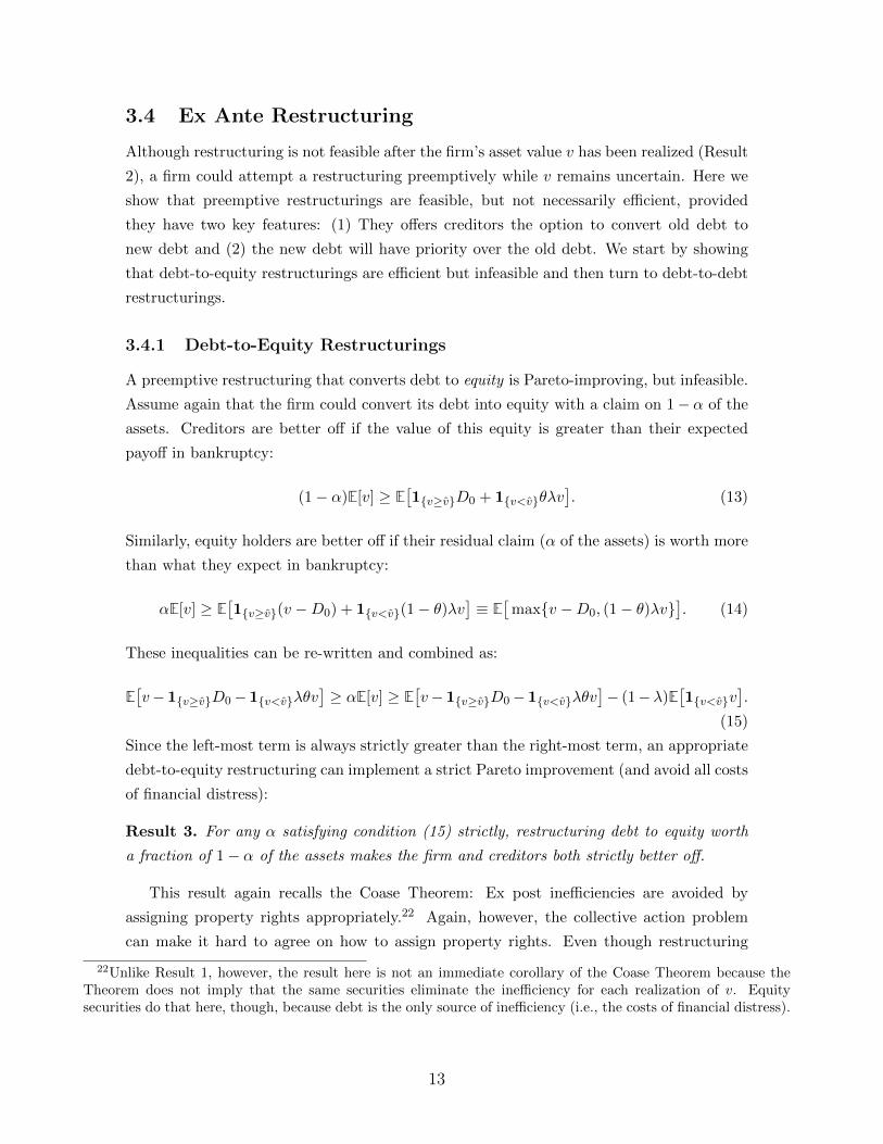
3.4 Ex Ante Restructuring

Although restructuring is not feasible after the firm’s asset value v has been realized (Result

2), a firm could attempt a restructuring preemptively while v remains uncertain. Here we

show that preemptive restructurings are feasible, but not necessarily efficient, provided

they have two key features: (1) They offers creditors the option to convert old debt to

new debt and (2) the new debt will have priority over the old debt. We start by showing

that debt-to-equity restructurings are efficient but infeasible and then turn to debt-to-debt

restructurings.

3.4.1 Debt-to-Equity Restructurings

A preemptive restructuring that converts debt to equity is Pareto-improving, but infeasible.

Assume again that the firm could convert its debt into equity with a claim on 1− α of the

assets. Creditors are better off if the value of this equity is greater than their expected

payoff in bankruptcy:

(1− α)E[v] ≥ E[1{v≥v}D0 + 1{v<v}θλv

]. (13)

Similarly, equity holders are better off if their residual claim (α of the assets) is worth more

than what they expect in bankruptcy:

αE[v] ≥ E[1{v≥v}(v −D0) + 1{v<v}(1− θ)λv

]≡ E

[max{v −D0, (1− θ)λv}

]. (14)

These inequalities can be re-written and combined as:

E[v−1{v≥v}D0−1{v<v}λθv

]≥ αE[v] ≥ E

[v−1{v≥v}D0−1{v<v}λθv

]− (1−λ)E

[1{v<v}v

].

(15)

Since the left-most term is always strictly greater than the right-most term, an appropriate

debt-to-equity restructuring can implement a strict Pareto improvement (and avoid all costs

of financial distress):

Result 3. For any α satisfying condition (15) strictly, restructuring debt to equity worth

a fraction of 1− α of the assets makes the firm and creditors both strictly better off.

This result again recalls the Coase Theorem: Ex post inefficiencies are avoided by

assigning property rights appropriately.22 Again, however, the collective action problem

can make it hard to agree on how to assign property rights. Even though restructuring

22Unlike Result 1, however, the result here is not an immediate corollary of the Coase Theorem because theTheorem does not imply that the same securities eliminate the inefficiency for each realization of v. Equitysecurities do that here, though, because debt is the only source of inefficiency (i.e., the costs of financial distress).

13

debt to equity can fully eliminate inefficiencies (i.e., the costs of financial distress), creditors

might not accept due to the same hold-out problem.

To see why, recall that an individual creditor accepts only if it is better off, given that

other creditors accept. That is, it must prefer getting a fraction 1−α of the assets to holding

its original debt with face value D0. If all other creditors agree to the restructuring, the

firm is effectively all equity (assuming the individual creditor is infinitesimally small). A

creditor therefore accepts if:

(1− α)E[v] ≥ D0. (16)

Similarly, equity holders are better off in a restructuring if their residual claim on the

fraction α of the assets is worth more than their bankruptcy payoff, as in inequality (14).

These inequalities can be re-written and combined as:

E[v]−D0 ≥ αE[v] ≥ E[v]−D0 + E[1{v<v}

{(1− θ)λv − (v −D0)

}]. (17)

The last expectation is positive, because the term in braces is positive for v < v by the

definition of v (equation (7)). Hence, the right-most term is greater than the left-most

term; no restructuring of debt to equity is feasible:

Result 4. There is no ex ante restructuring of debt to equity that (uncoordinated) creditors

are willing to accept and the firm is willing to offer.

Intuitively, although exchanging debt for equity allows the firm to avoid distress completely,

it is too expensive because it must induce creditors to give up debt which is effectively

default free, given they condition their decisions on the exchange being successful.

3.4.2 Debt-to-Debt Restructurings

So far, we have assumed that the firm’s creditors have equal priority in bankruptcy, sharing

pro rata in any distribution of assets. In practice, a firm can issue debt with different

levels of seniority. The value of seniority is that, in the event of liquidation or bankruptcy,

senior creditors must be paid before junior creditors receive anything. As we will show

below, ex ante restructuring becomes feasible when the firm is able to issue senior debt.

By offering to exchange senior debt (with a lower face value) for existing junior debt, the

firm can induce individual creditors to assent to the restructuring because hold-outs will

be diluted.23 This kind of restructuring is feasible ex ante (when v is still uncertain) but

not ex post (when v is realized). Ex post, individual creditors do not gain from giving

up (i) low-priority, high-face-value claims for (ii) high-priority, low-face-value claims if the

restructuring eliminates the risk of a bankruptcy filing. Assuming all other creditors agree

23Optimal “dilutable debt” also appears in Diamond (1993), Donaldson, Gromb, and Piacentino (2020b, 2020a),Donaldson and Piacentino (2020), and Hart and Moore (1995).

14

to the restructuring, the individual creditor should retain its original (low-priority) claim,

which will be paid in full after the restructuring. Priority, in other words, is only as valuable

as a bankruptcy is likely. This is why a debt-for-debt restructuring is feasible ex ante, when

v is uncertain: Even after a restructuring, a bankruptcy filing is still possible in the future

because restructuring prevents distress for some but not all realizations of v. Priority is

therefore valuable: It puts senior creditors ahead of junior creditors if a bankruptcy occurs.

We begin by showing the feasibility of a restructuring that swaps old debt (D0) for more

senior debt (D). An individual creditor will accept this restructuring if the value of senior

debt with face value D is greater than the value of junior debt with face value D0, given

that other creditors are accepting the terms of the restructuring:(1− F

(v(D)

))D + F

(v(D)

)E[θλv

∣∣ v < v(D)]≥(

1− F(v(D)

))D0. (18)

The right-hand side of the inequality measures the expected payoff to junior debt, which is

paid D0 if there is no future default and zero otherwise. The reason the payoff is zero in

default is that in bankruptcy not all debt is paid in full (D > v by equation (7)) and, since

all other debt is senior, the payoff to junior debt is zero.24

Equity holders will also accept a restructuring—swapping junior debt for senior debt—if

their residual claim on the assets is more valuable than their expected payoff in the absence

of a restructuring. Note that the seniority of debt has no effect on the payoff to equity:

Whether debt is senior or junior, it still has priority over equity. This means that equity

holders will accept the restructuring whenever it reduces the face value of the debt, or

D ≤ D0.

Rearranging these inequalities, we obtain the following result, which describes the fea-

sibility of a restructuring that reduces the face value of debt by D0 −D:

Result 5. For any D such that

D0 −D ≤F(v(D)

)1− F

(v(D)

)E[θλv

∣∣ v ≤ v(D)], (19)

restructuring the initial debt D0 to senior debt with face value D < D0 is accepted by

creditors and makes the firm strictly better off.

Inequality (19) makes clear that the feasibility of a restructuring increases with both (i)

the likelihood of a bankruptcy filing F (v) and (ii) creditors’ recovery value in default

E[θλv

∣∣ v ≤ v(D)]. This is intuitive because both increase the value of priority. Indeed, if

a firm never goes bankrupt, priority has no value—even the last creditor will be repaid in

24We are assuming that senior debt is always paid ahead of junior debt. That is, there are no deviations fromthe APR that favor junior creditors at the expense of senior creditors. Although this assumption appears to be agood approximation of reality (Bris, Welch, and Zhu (2006)), we relax it in Section 5.1. Moreover, we show thatdeviations favoring junior creditors at the expense of senior debt are suboptimal from a welfare point of view.

15

full. And, similarly, if creditors’ recovery value is low, priority has no value—even the first

creditor might not be repaid in full. These two pieces underlie all of our main results.

Building on this result, we explore how the parameters of the bankruptcy environment—

deadweight costs (λ) and creditor friendliness (θ)—affect the ability to restructure. Despite

the intuitive pieces underlying them, the comparative statics can be counter-intuitive be-

cause θ and λ affect restructuring not only directly, but also indirectly via v (cf. equation

(7)).

Before turning to comparative statics, we pause to note that, although restructuring in-

creases efficiency because it decreases financial distress costs, it is possible (at least theoret-

ically) that a restructuring will not yield a Pareto improvement. It could instead constitute

a “coercive exchange” in which creditors accept a restructuring that makes them worse off

because they want to avoid being diluted by new senior debt. This so-called “hold in” prob-

lem appears to be more of a theoretical possibility than a practical reality. Restructurings

generally do not harm creditors (Chatterjee, Dhillon, and Ramarez (1995)). Additionally,

restructurings do implement Pareto improvements in our model whenever distress is suf-

ficiently costly because, in such a case, creditors benefit more from avoiding distress than

they suffer from write-downs.25

3.5 Write-downs and Secured Credit Spreads

Before turning to comparative statics, we pause to interpret the bound on the feasible write-

down D0 − D (inequality (19)) in terms of market prices. To do so, we can re-write the

condition for creditors to accept a restructuring (inequality (18)) in terms of continuously

compounded yields-to-maturity, ys and yu, conditional on the write-down:

De−ys ≥ D0e

−yu . (22)

25It may be useful to illustrate how a marginal decrease in debt can still make creditors better off, becausethey prefer to get paid a smaller amount with higher probability than a larger amount with lower probability.Creditors with debt D0 are better off decreasing debt if

∂

∂D

∣∣∣∣D=D0

((1− F

(v(D)

))D + F

(v(D)

)E[λθv

∣∣ v < v(D)])

< 0 (20)

or, computing,1− F

(v(D0)

)f(v(D0)

)v(D0)

<1− λ

1− (1− θ)λ. (21)

Let us make two observations. (i) The condition can be satisfied only if λ is sufficiently small: If λ = 1, thereare no bankruptcy costs to avoid by reducing debt, so creditors are always better off with more debt. (ii) Itcan be satisfied more easily when f

(v(D0)

)is large—that is, when a small reduction in debt from D0 has a

significant impact on the probability of default. At any rate, even if they do not implement Pareto improvements,restructurings do always increase total surplus in our model.

16

Here, ys is the yield on secured/senior debt (which creditors receive in a restructuring);

yu is the yield on unsecured/junior bonds (which they exchange). This is equivalent to:

log

(D0

D

)≤ yu − ys. (23)

The left-hand side is approximately the proportion of debt that can be written down (D0−D)/D0. The right-hand side is the spread between secured and unsecured credit. We thus

have the following approximation:26

max % write-down ≤ secured credit spread. (25)

This inequality captures the basic intuition of the hold-out problem in our model. Creditors

are willing to accept write-downs only to the extent that seniority is valuable (as measured

by the secured credit spread). The inequality also suggests a way to estimate feasible

write-downs. Secured credit spreads are, in principle, observable.27

Benmelech, Kumar, and Rajan (2020) find that for distressed (low-rated) firms, the

secured-unsecured spread is about six percent annualized on bonds with maturity of about

seven years, making the unannualized spread yu − ys, and, by inequality (25), likewise our

estimate of the maximum write-down, equal to about 42 percent. This seems to accord

with the data: Studying distressed exchanges of unsecured for secured debt, Mooradian

and Ryan (2005) find a mean write-down of 44 percent.

Finally, inequality (25) offers an unusual perspective on the timing of restructuring.

Observed spreads are substantial only when firms are in trouble (Benmelech, Kumar, and

Rajan (2020)). Thus, debt restructuring could be rare in good times not only because it

is not valuable (because expected distress costs are low), but also because it is infeasible

(because secured credit spreads are low).

3.6 How the Costs of Bankruptcy Affect Restructuring

A restructuring is feasible if the debt write-down, D0 − D, satisfies the constraint in in-

equality (19). The maximum feasible write-down renders this an equality. Here we explore

how the maximum feasible write-down varies with the deadweight costs of bankruptcy (λ).

Is the new face value D that makes creditors indifferent between accepting and rejecting a

restructuring—which makes inequality (19) bind—increasing or decreasing in λ?

26Using log(1− x) ≈ −x, we can re-write the left-hand side of inequality (23):

log

(D0

D

)= − log

(1− D0 −D

D0

)≈ D0 −D

D0. (24)

27Although, to be precise, the spread must be conditional on successful restructuring. Additionally, to measurethe spread in practice, the firm must have some other debt that is not restructured.

17

Define an individual creditor’s gain from restructuring relative to bankruptcy, given

others accept, as ∆. Using inequality (19), we can write ∆ as follows:

∆ :=(

1− F(v(D)

))(D −D0

)+ F

(v(D)

)E[θλv

∣∣ v < v(D)]. (26)

This is the creditors’ incentive compatibility constraint (IC). The maximum write-down, or

lowest face value D∗, corresponds to ∆ = 0. Differentiating D∗ with respect to λ, we obtain

the next result:

Result 6. Bankruptcy Costs: Reducing bankruptcy costs (increasing λ) facilitates re-

structuring in the sense that the maximum write-down D0 −D∗ is increasing in λ.

This is a central result of our paper: Restructuring and bankruptcy are complements, not

substitutes. This is true for two reasons:

1. The more efficient bankruptcy is, the more likely the firm is to file, and priority in

bankruptcy is more valuable when it is more likely.

2. The more efficient bankruptcy is, the more creditors get in bankruptcy, and priority

in bankruptcy is more valuable when recovery values are higher.28

In other words, as bankruptcy costs fall, priority in bankruptcy becomes more valuable,

which increases the likelihood that creditors will accept write-downs in exchange for priority.

Hence, contrary to common intuition, policies that reduce bankruptcy costs actually facil-

itate out-of-court restructuring. This adds support to Brunnermeier and Krishnamurthy’s

(2020, p. 6) conclusion that “reducing the cost of bankruptcy is unambiguously beneficial

to society.”

3.7 How the Creditor Friendliness of Bankruptcy Affects Re-

structuring

The feasibility of a restructuring also depends on the creditor friendliness of the bankruptcy

system. As in the previous subsection, we focus on the maximum feasible write-down, D∗,

corresponding to ∆ = 0 in equation (26). Differentiating D∗ with respect to θ, we obtain

our next result:

Result 7. Creditor friendliness: An increase in creditor friendliness (θ) facilitates

restructuring, in the sense that the maximum feasible write-down D0−D∗ increases, if and

28To see why, recall, from the IC in inequality (18), that creditors accept a restructuring only if the payoff theyget in bankruptcy from accepting senior debt is high relative to the payoff they get in bankruptcy from holdingout, which, conditional on others accepting, is zero. Thus, as senior creditors’ payoff in bankruptcy increases, sodoes the write-down creditors are willing to accept.

18

only if ∂∆/∂θ is positive (see equation (53) in the Appendix). Moreover, if

1− F(D∗θ=1

)D∗θ=1f

(D∗θ=1

) < λ, (27)

where D∗θ=1 denotes the solution to ∆ = 0 with θ = 1, then there is an interior level of

creditor friendliness θ∗ ∈ (0, 1) that maximizes the feasible write-down.

The ambiguity in this result stems from the fact that, although restructuring is facilitated

when priority in bankruptcy becomes more valuable, creditor friendliness has two effects

on the value of priority:

1. By increasing what creditors receive in the event of bankruptcy, creditor friendliness

makes priority more valuable.

2. By reducing the payoff to equity holders, creditor friendliness reduces their incentive

to file for bankruptcy, which makes priority less valuable.

Condition (27) is important because it tells us that, when creditor friendliness is very high

(θ is near 1), further increases in θ reduce the likelihood of a successful restructuring. This

implies that the optimal level of creditor friendliness is less than 1 (θ∗ < 1). In other words,

the optimal bankruptcy system does not maximize creditor recoveries.29 Systems that are

too creditor friendly are inefficient because they discourage cost-reducing restructurings.

The U.S. may be one such system, as we illustrate in the next section. Before that, however,

we illustrate the result above with an example.

3.7.1 Example: Optimal Creditor Friendliness If v Is Uniform

Here, we illustrate the results above for v uniform, F (v) ≡ v/v on [0, v]. In this case,

creditors’ binding IC (∆ = 0 in equation (26)) becomes:

λθ

2v

(v(D∗)

)2= (D0 −D∗)

(1− v(D∗)

v

). (28)

Substituting for v from equation (7) and solving gives:30

D∗ =

(1− (1− θ)λ

)v +D0 −

√(D0 −

(1− (1− θ)λ

)v)2

+ 2λθvD0

2− λθ1−(1−θ)λ

. (29)

This expression illustrates that the write-down D0−D∗ is increasing in λ, as per Result 6,

and is hump-shaped in θ, as per Result 7; see Figure 1.

29Bisin and Rampini (2005) uncover a related downside of creditor friendliness: By discouraging filings, lowbankruptcy payoffs to equity can make it hard for a bank to enforce exclusive contracts.

30The other root of the quadratic is larger than D0 and is omitted.

19

.2 .4 .6 .8 10%

5%

10%

15%

20%

creditor friendliness θ →

%write-dow

nD

0−D∗

D0

→

Figure 1: The percentage write-down for uniform v on [0, v], with v = 100, D0 = 50, and λ = 1/2.

3.8 Is the U.S. Bankruptcy Code Too Creditor Friendly?

We can use our model to assess whether existing laws are excessively creditor friendly in

the sense that a marginal reduction in creditor friendliness would increase the feasibility

of restructurings. To do this, we assume that D∗ is a continuous function of θ with a

unique local minimum.31 Under this assumption, we can say that a bankruptcy system is

too creditor friendly if an increase in θ leads to an increase in D∗, the minimum debt level

attainable in restructuring:∂D∗

∂θ> 0. (30)

In Appendix B.2, we calculate that a sufficient condition for this inequality to hold is:

1 < λθv∂F (v)

∂D. (31)

Focusing on the terms on the right-hand side, this condition says that the Code is too

creditor friendly if (i) creditors’ total recovery value for the marginal bankruptcy firm is

already high (i.e., λθv is high), or (ii) the likelihood that the firm files is highly sensitive to

its indebtedness (∂F/∂D is high). When λθv is already high, the marginal value of a further

increase in recovery value is low. When ∂F/∂D is high, the marginal value of a decrease in

debt is high. That is, even a small reduction in the face value of debt, via a restructuring,

would yield a large reduction in the probability of bankruptcy, thereby avoiding deadweight

costs.

A back-of-the-envelope calculation allows us to get a preliminary sense of whether con-

31That is, an increase in creditor friendliness either always increases, always decreases, or first increases andthen decreases the maximum feasible write-down (based on numerical examples, we think that this assumptionis satisfied for commonly-used distributions).

20

dition (31) is satisfied in the U.S. today. The empirical literature provides approximations

for each term on the right hand side:

• λ: This term captures the direct costs of bankruptcy. In studies of corporate reorga-

nizations (mostly involving large corporations), the literature consistently estimates

λ > 90 percent. (See Hotchkiss et al. (2008), Table 1, for a summary of twelve studies.)

• θ: A number of papers investigate the value retained by equity holders in bankruptcy.

They suggest θ > 85 percent is a conservative lower bound—in most cases, creditors

are paid in full before equity is paid anything. (See Hotchkiss et al. (2008), Section

5.1, for a summary of estimates.)

• v∂F (v)/∂D: To approximate this term, suppose a firm is near bankruptcy, in the

sense that the current value of assets, which we denote by v0, is close to the threshold

v. In this case, we can write:

v∂F (v)

∂D≈ ∂F (v)

∂(D/v0). (32)

This term thus measures the sensitivity of the default probability to the level of

leverage, D/v0 (holding the current value of assets constant). An estimate of this

sensitivity can be derived from Campbell, Hilscher, and Szilagyi (2008). In a logistic

regression of the bankruptcy-filing probability against leverage (and other controls,

including market capitalization), the authors estimate a coefficient on leverage equal

to 5.38. Using the “divide-by-four” rule (Gelman and Hill (2007)), this coefficient

translates to an approximate marginal effect equal to 1.35. We view this as a con-

servative lower-bound estimate of condition (32) for two reasons. First, Campbell,

Hilscher, and Szilagyi (2008) study bankruptcies within the next month, whereas our

model applies to bankruptcies over a longer horizon, corresponding to the maturity of

restructured bonds.32

Second, they study a sample of healthy and distressed firms, whereas our model per-

tains to distressed firms. The sensitivity of bankruptcy to leverage is likely highest for

distressed firms. Indeed, healthy firms take on leverage for a variety of reasons, such

as financing profitable investments or controlling managerial free cash-flow problems,

32It is actually not unconditionally true that the sensitivity of the bankruptcy probability to leverage is increas-ing in maturity. But it is for sufficiently short maturities, and the maturities here are almost surely sufficientlyshort. To see why, suppose that the probability of filing before time T is given by a Poisson distribution:P[bankruptcy by T ] = 1 − e−πT , where π represents the filing intensity, taken as a proxy for leverage (althoughit suffices that it be an increasing function of it). Differentiating, we find that the sensitivity of the probabilityto π is Te−πT . This is first increasing, then decreasing, in T , with a maximum at T ∗ = 1/π. Now, we can useour motivating fact that seventeen percent of firms file for bankruptcy within three years after a restructuring(Moody’s (2017)) to estimate T ∗: 1 − e−3π = 17% =⇒ π ≈ 6.2% and T ∗ ≈ 16 years. This is longer than thetypical debt maturity, implying that the sensitivity is increasing for relevant horizons and, thus, that Campbell,Hilscher, and Szilagyi’s (2008) short-horizon estimate is a lower bound on what we need.

21

that could even be negatively related to the probability of bankruptcy.

Taking these numbers at face value, we can calculate the right-hand side of condition (31):

λθv∂F (v)

∂D> 90%× 85%× 135% ≈ 103%. (33)

This is greater than one, implying that the condition (31) is satisfied in the U.S. Note

that this condition is sufficient, but far from necessary, and that the numbers we plug in

are conservative. This leads us to believe that current law is likely too creditor friendly.

Giambona, Lopez-de Silanes, and Matta (2019) provide evidence supporting this conclusion.

They find that an exogenous increase in creditor protection led to an increase in bankruptcy

filings. This could be surprising because nearly all bankruptcies are initiated by debtors—

why should they file bankruptcy more often when they expect less in bankruptcy?—but it

is consistent with our calculations, which show that creditor-friendly bankruptcy rules can

impede restructuring, resulting in more bankruptcies.33

4 Relief Policy

Here, we turn to the policy implications of our model. We consider the vantage point of a

(utilitarian) social planner choosing how to allocate a marginal dollar (“subsidy”). We think

this is a useful exercise because, during the ongoing COVID-19 pandemic, policymakers

have implemented subsidies to aid firms outside of bankruptcy (e.g., the CARES Act) and

various commentators have proposed programs to aid firms in bankruptcy (e.g., DeMarzo,

Krishnamurthy, and Rauh (2020)). We begin by showing that the social planner must take

into account not only the effect of the subsidy on the likelihood of financial distress, but also

its effect on restructuring. Then, we consider specific policies, including subsidies granted

unconditionally, conditional on restructuring, and conditional on bankruptcy. Finally, we

compare these policies and show that the most effective policies are those that facilitate

restructuring either by subsidizing it directly or by subsidizing bankruptcy.

4.1 Planner’s Problem for a Marginal Dollar

In our model, social welfare is firm value. Since firm value is maximized when the default

probability F (v) is minimized, the planner’s objective is simply to minimize v. We denote

33This finding—that U.S. law has become too creditor friendly—may help explain another pattern in the data.Adler, Capkun, and Weiss (Adler et al.) find that, among firms filing for Chapter 11, average asset values fell andleverage increased during a period (1993–2004) when creditor control substantially increased. These findings areconsistent with our model: As the law becomes excessively creditor friendly, the threshold for filing for bankruptcy(v) declines for any given level of debt (see inequality (7)). In other words, among firms filing for bankruptcy,asset values decline as creditor-friendliness increases, holding debt constant. And as asset values decline, relativeto D, firms in bankruptcy have higher leverage.

22

the set of subsidies the planner can deploy by the vector s and their associated costs by

q. For example, si could capture a direct subsidy to the firm’s assets, such as cash grants

or forgivable loans (both of which have been deployed during the pandemic). In this case,

qi = 1, because the planner pays a dollar to increase the firm’s assets by a dollar. Similarly,

sj could capture a subsidy to the firm’s assets conditional on filing for bankruptcy. In this

case, qj = F (v), because the planner pays a dollar to increase the firm’s assets by a dollar

only if the firm files for bankruptcy, which happens with probability F (v). Thus, if the

planner’s budget is ε, its budget constraint is q · s = ε.

Although we allow the planner to make its subsidies contingent on bankruptcy and re-

structuring, we do not allow it to force creditors to discharge debt outside of bankruptcy.

Put differently, the planner must respect creditors’ IC, shown in inequality (18) (equiva-

lently, ∆(s) = 0).

Thus, the planner’s problem is:min v(s)

s.t. ∆(s) = 0

& q · s = ε

(34)

over feasible subsidies s.

Because we are interested in how the planner can best spend a marginal dollar, we focus

on ε near zero. Writing the optimal policy as a function of the budget, s = s(ε), we can

approximate the social planner’s objective as:

v(s(ε)

)= v(s(0)

)+ ε

d

dεv(s(0)

). (35)

This captures the idea that the planner can allocate its budget little by little: It should select

subsidies to maximize the marginal impact on the objective—to maximize dv/dε—subject

to the creditors’ IC (∆(s) = 0).

Below, we analyze and compare policies. As a shorthand, we let si be the policy that

gives subsidy si to the ith policy and nothing to the others. For such one-dimensional

policies, the planner’s objective is to minimize

dv

dε

∣∣∣∣ε=0

=∂v

∂si

dsidε

∣∣∣∣ε=0

, (36)

over feasible policies si, subject to the constraints. This expression lends itself to interpre-

tation. Begin with the second term on the right-hand side (dsidε ). If we differentiate the

23

budget constraint, we see that this term is the reciprocal of the cost of the ith policy,

dsidε

=1

qi. (37)

The planner’s objective is therefore:

∂v

∂si

∣∣∣∣si=0

× 1

qi≡ “policy efficacy” × “bang for the buck” (38)

subject to creditors’ IC.

This IC plays a central role in our policy analysis below. The planner must account

for the effect of each policy on creditors’ private incentives to accept a restructuring. To

see how, observe that both v and the IC depend on the equilibrium level of debt post-

restructuring, which in turn depends on the subsidy scheme: D = D(s). Taking this into

account and applying the chain rule twice, we can re-write the objective as:

dv

dε

∣∣∣∣ε=0

=

(∂v

∂si+∂v

∂D

∂D

∂si

)1

qi

∣∣∣∣si=0

(39)

=

(∂v

∂si− ∂v

∂D

∂∆/∂si∂∆/∂D

)1

qi

∣∣∣∣si=0

. (40)

The first term captures the direct effect of a subsidy. But it is far from the whole story.

The second term captures its indirect effect via restructuring: The product of how the debt

level affects the default threshold ( ∂v∂D ) and how the subsidy affects the debt level via the

IC (∂∆/∂si∂∆/∂D ), all times the “bang for the buck” (1/qi).

4.2 Feasible Policies

We use expression (40) to evaluate two groups of policies: ex post policies that target firms

in bankruptcy and ex ante policies that target firms prior to bankruptcy. Ex post policies

have the advantage of lower fiscal costs (due to the lower probability of actually paying the

subsidy), but the potential disadvantage of distorting firms’ decisions, as we characterize

below.

Ex post policies include:

1. Asset subsidies. These include, for example, cash subsidies to firms in bankruptcy.

2. Equity subsidies. These include policies that permit shareholders to retain own-

ership interests during a bankruptcy reorganization. For example, small-business

bankruptcy laws were recently amended to permit reorganization plans that allow

owners to retain their interests, as discussed in Morrison and Saavedra (2020).

3. Loan subsidies. These policies increase both assets and debt by extending credit

at below-market rates. One example is DeMarzo, Krishnamurthy, and Rauh’s (2020)

24

proposed debtor-in-possession financing facility (DIPFF), which would offer subsidized

financing to firms in bankruptcy. The distributional impact of these subsidies depends

on the priority of the new loans: If the loans are junior to senior debt, they are a

subsidy to senior debt; if they are senior to existing debt, they function as a subsidy

to equity. Below we focus on ex post loan subsidies that benefit creditors.

Ex ante policies are similar, but broader in scope:

4. Asset subsidies. These include include cash grants (such as those paid to the airlines

under the CARES Act) and forgivable loans (such as those paid under the Paycheck

Protection Program).

5. Loan subsidies. These include the various facilities launched by the Federal Reserve

during the current crisis (e.g., Primary Market Corporate Credit Facility, Main Street

Lending Program).

6. Debt subsidies. These policies reduce debt by repurchasing it at the market price

(before restructuring) and then forgiving it. They bear some resemblance to quanti-

tative easing programs in which central banks purchase corporate debt, with the twist

that the central bank then does not enforce repayment on the debt.

7. Restructuring subsidies. The government could simply reward creditors who par-

ticipate in a restructuring. One way to do this is to alter the tax consequences of

restructurings, as discussed in Campello, Ladika, and Matta (2018). Another is for

the government to announce that, if creditors agree to write-downs, the government

will agree to even larger write-downs of its own claims, as discussed in Blanchard,

Philippon, and Pisani-Ferry (2020).

In Appendix B.3, we formalize these policies. For each Policy i, we describe its direct

cost qi (the probability the subsidy is paid), its direct effect via the filing decision (the

change in the bankruptcy threshold v), and its indirect effect via restructuring (the way

D is affected through the IC). We find that we can rank the policies by simply comparing

dvsi/dε for each policy. This leads to our next result:

Result 8. Policy Comparison: Ex ante debt subsidies (Policy 6) and restructuring

subsidies (Policy 7) are equivalent to ex post loan subsidies (Policy 3) and are strictly

preferred to all other policies. Further, ex ante asset subsidies (Policy 4) are preferred

to both ex ante subsidized lending (Policy 5) and ex post bankruptcy subsidies for equity

(Policy 2). Finally, ex post bankruptcy subsidies for assets (Policy 1) are preferred to ex

post bankruptcy subsidies for equity (Policy 2). (The rest of the ranking is ambiguous.)

In other words, the best policies—ex ante restructuring subsidies, ex ante debt purchases,

and ex post loan subsidies—are those that facilitate restructuring alone. Indeed, none of

25

these policies has any direct effect on filing: Each affects welfare indirectly by increasing

creditors’ payoff from accepting a restructuring by ε, thereby slackening the IC:

• Because restructuring subsidies (Policy 7) go directly to creditors who accept restruc-

turing, they increase creditors’ payoff from accepting by ε. This mechanically slackens

the IC by ε.

• Ex post loan subsidies (Policy 3) increase the value of priority. This is because, if

creditors accept a restructuring, they get the entire asset value in bankruptcy. The

subsidies are similar to a reduction in the costs of bankruptcy borne by creditors. It

turns out that this slackens the IC by ε.34

• Debt subsidies (Policy 6) decrease each creditor’s initial debt.35 Because of this, they

decrease creditors’ payoff from holding out. It turns out this slackens the IC by ε.36

5 Extensions

5.1 Secured Creditor Power and Priority Rules

We have assumed thus far that senior debt is paid strictly before junior debt in bankruptcy.

In other words, there are no deviations from the “absolute priority rule” (APR) that favor

unsecured creditors at the expense of secured creditors.37 Although this is a good first

approximation, in practice the division of surplus between secured and unsecured creditors

depends on post-filing decisions, such as the decision to liquidate or reorganize. Liquidation

is likely to favor secured creditors who seek quick payouts, whereas reorganization is likely

to favor unsecured creditors who want to gamble on the going concern. (Other decisions

affecting the division of surplus include whether to incur post-petition (DIP) financing,

liquidate assets or the entire firm, or litigate priority disputes.) And, even though all

bankruptcy decisions are overseen by a bankruptcy judge, many scholars have shown that

secured creditors exert substantial influence over the bankruptcy process.

34These subsidies increase creditors’ payoff from accepting senior debt by F · s3, where F is the probability ofbankruptcy. Given s3 = ε/F (q3 = F in the planner’s budget constraint), this slackens the IC by ε.

35Here, we interpret the subsidy as decreasing each creditor’s debt by, for example, buying a small amountfrom every debt holder. We could also interpret it as decreasing the total amount of debt by, for example, buyingall the debt of a small number of debt holders. The two interpretations are mathematically equivalent, but givedifferent perspectives on the creditors’ IC. The latter slackens the IC because it sweetens the deal from accepting,since the bankruptcy payoff is divided among fewer creditors. In contrast, the former slackens the IC because itsours the deal for hold-outs, as described above.

36The policy decreases creditors’ payoff from holding out by (1 − F )s6, where 1 − F is the probability ofrepayment. Given s6 = ε/(1− F ) (q6 = 1− F in the planner’s budget constraint), this slackens the IC by ε.

37At the same time, we have assumed that equity recovers something in bankruptcy ((1 − θ)λv) even if debtis not paid in full. We have, in other words, assumed that there are deviations from the APR that favor equityat the expense of debt. Our analysis above suggests that high θ could impede restructuring (Result 7). Thismeans that violations of debt-equity priority can be optimal. Here we show the opposite is true for violations ofsecured-unsecured priority: They make restructuring harder.

26

Here, we extend the model to capture different levels of secured creditor power, which

we denote by ρ. Specifically, as in the baseline model, we assume that there are two classes

of debt—senior/secured and junior/unsecured. Unlike the baseline model, however, we also

assume that senior creditors are more likely to be paid first as their power (ρ) increases.

Specifically, we assume that senior debt is paid first with probability ρ, but shares pro-

rata with junior debt with probability 1 − ρ (i.e., they are treated as if they are equal in

priority). We still assume that equity gets a fraction 1−θ of the value in bankruptcy. What

is changing here is how the fraction θ is divided among creditors.38

To explore how ρ affects restructuring, we start with the creditors’ IC to accept a write-

down from D0 to D:(1− F

(v(D)

))D + F

(v(D)

)E[θλv

∣∣ v < v(D)]

≥(

1− F(v(D)

))D0 + (1− ρ)F

(v(D)

)E[θλv

∣∣ v < v(D)] D0

D.

(41)

The difference between the above and condition (18) is that, with probability 1−ρ, a hold-

out creditor’s junior debt receives a positive recovery value in bankruptcy (an accepting

creditor’s payoff is unchanged because it takes as given that others accept). Rearranging,

we see that a write-down D −D0 is feasible if:

D0 −D ≤θλF

(v(D)

)1− F

(v(D)

)E[v∣∣ v ≤ v(D)

](1− (1− ρ)

D0

D

). (42)

This is identical to the original feasibility condition (19) except for the final expression

in brackets on the right-hand side. Indeed, when the APR is enforced strictly (ρ = 1),

inequality (42) reduces to the original feasibility condition. Because the right-hand side is

increasing in ρ, we have the next result:

Result 9. Strict enforcement of the priority of senior over junior debt, i.e. ρ = 1, facilitates

restructuring, in the sense that it maximizes the feasible write-down in inequality (42).

This suggests a counterpoint to arguments that the APR between secured and unsecured

debt should be relaxed (e.g., Bebchuk and Fried (1996)). Advocates of this view often

emphasize that the APR gives secured debt power to dilute unsecured debt. Our model

reflects this power, but suggests that this power is not necessarily inefficient because it

facilitates restructuring and thereby helps circumvent financial distress. Thus, our model

helps rationalize observed practice: Equity–debt violations are more common than secured–

unsecured violations (Bris, Welch, and Zhu (2006)).

38Although we interpret creditor power mainly as a policy parameter describing the bankruptcy code or judicialpreferences, it could also reflect market forces. Notably, Jiang, Li, and Wang (2012) find that when firms’unsecured debt is held by hedge funds, total payoffs to creditors tend to increase in bankruptcy (our θ is higher)and so do payoffs to unsecured creditors (our ρ is lower). Thus, our analysis suggests a possible downside of hedgefund participation in debt markets: It can make restructuring harder (see Section 3.8 and Result 3.8).

27

We now ask how secured creditor power affects the write-down-maximizing level of

creditor friendliness: If secured creditors get more relative to unsecured creditors (ρ is

higher), should creditors as a whole get more or less relative to equity (i.e., should θ be

higher or lower) to maximize the write-down D0 −D? We find that they should get more:

Result 10. Suppose that the write-down is maximized at a unique interior level of creditor

friendliness θ∗ that is not an inflection point (as in, e.g., the uniform case in Figure 1).

Increasing the secured creditor power ρ increases the optimal level of creditor friendliness.

That is, dθ∗/dρ > 0.

To see the intuition for this result, recall that θ∗ is chosen to maximize the value of priority,

balancing the increase in creditor recovery value against the decrease in the filing probability.

Because high secured creditor power ρ increases recovery value without affecting the filing

probability, θ∗ increases to balance the two effects.

5.1.1 Inefficiencies of Secured Creditor Control

Our analysis so far has assumed that secured creditor control amounts to a transfer from

unsecured creditors. It could instead reduce total surplus. For example, secured creditors

could force quick sales, potentially at fire sale prices, at the expense of other claimants as

Ayotte and Ellias (2020), Antill (2020), and Ayotte and Morrison (2009) document. In light

of this evidence, we now relax the assumption that liquidation costs do not depend on the

division of surplus. We assume instead that secured creditor power can lead to inefficient

liquidation.

To capture the inefficiencies resulting from secured creditor power, we assume that

unsecured debt gets only a fraction ζ of what is left after secured debt and equity are paid.

Thus, 1− ζ captures the inefficiency of secured creditor power. With this modification, the

creditors’ IC in equation (41) becomes(1− F

(v(D)

))D + F

(v(D)

)E[θλv

∣∣ v < v(D)]

≥(

1− F(v(D)

))D0 + ζ(1− ρ)F

(v(D)

)E[θλv

∣∣ v < v(D)] D0

D.

(43)

Observe that ζ above plays exactly the same role as 1 − ρ in equation (42). Therefore,

Results 9 and 10 imply that an increase in ζ makes restructuring harder and reduces the

optimal level of creditor friendliness θ∗. In words, the inefficiencies of secured creditor power

1 − ζ are actually good for restructuring and suggest that a more creditor-friendly Code

is optimal. The intuition mirrors that for the results above: As the bankruptcy payoff to

unsecured debt decreases, their payoff from holding out decreases, inducing them to accept

write-downs.

But what happens when secured creditor power imposes inefficiencies on equity holders?

28

We address this question in Appendix B.4 and show that, more conventionally, the Code

should be less creditor friendly when creditors impose greater deadweight costs.

5.1.2 Tort claimants

Priority rules appear in another place in policy debates: Should tort claimants—“accidental”

or “involuntary” creditors—be treated on par with or ahead of other creditors in bankruptcy?

Our model allows us to evaluate the effects of alternative priority rules on the likelihood of

restructuring before bankruptcy.

To address this question in reduced form, suppose the firm has outstanding tort claims

equal to T . If T is not paid in full prior to a bankruptcy filing, different priority rules

correspond to different types of taxes in bankruptcy: If tort claims are treated on-par with

secured claims, they are equivalent to tax τs on senior debt. If they are treated on-par with

unsecured debt, they represent a tax τj on junior debt. If they are junior to unsecured

debt, there is no tax on creditors (and they will often go unpaid).

With this set-up, we can return to creditors’ incentive to accept a restructuring. Their

IC becomes:(1− F (v(D + T ))

)D + F

(v(D + T )

)E[(1− τs)θλv

∣∣ v < v(D + T )]≥(

1− F (v(D + T )))D0 + (1− ρ)F (v(D + T ))E

[(1− τj)θλv

∣∣ v < v(D + T )] D0

D.

(44)

This condition is easiest to satisfy if τs is small and τj is large. This suggests that, to

facilitate restructuring, tort claimants should be paid behind secured debt, but ahead of

unsecured debt. That ordering makes priority valuable by increasing (i) the value of se-

cured debt and (ii) decreasing the value of unsecured debt. Put differently, by giving tort

claimants priority above junior debt but below senior debt, the law increases the difference

in payoffs between junior and senior debt. This makes priority more valuable and facilitates

restructuring.

5.2 Court Congestion

We have assumed thus far that the costs of bankruptcy do not depend on whether restruc-

turing occurs. This is reasonable for an individual firm because a single restructuring is

unlikely to affect the efficiency of courts. However, taken in aggregate, restructurings can

affect the costs of bankruptcy—if there are more out-of-court restructurings, fewer firms

will file for bankruptcy, and courts are likely to be less congested and more efficient. In

this section, we allow the costs of bankruptcy to be increasing in the number of firms that

file and we show that this creates a feedback loop that amplifies the effects of bankruptcy

costs on the hold-out problem.

29

We assume a unit of identical firms and that the costs of bankruptcy increase with the

number of firms that file. By the law of large numbers, the number of firms that file for

bankruptcy is equal to the probability that any individual firm files, or F (v). We assume

that a bankruptcy court can receive a maximum number of filings (κ) before experiencing

“congestion costs” that increase the deadweight costs of bankruptcy (see, e.g., Iverson

(2018)). A simple way to express this idea is to write bankruptcy costs as follows:

bankruptcy costs = 1− λH − 1{F (v)>κ}(λL − λH), (45)

which says that bankruptcy costs are equal to 1− λH if the number of bankruptcies F (v)

is below the threshold “court capacity” κ and increase to 1−λL if they are above it. When

κ = 1, this corresponds to the baseline model with λ = λH ; when κ = 0. it corresponds to

the baseline model with λ = λL.

We can analyze the effects of congestion on the feasibility of restructuring by appealing

to Result 6: High bankruptcy costs impede restructuring, making it hard to reduce debt,

and hence making bankruptcy itself more likely. This can create an amplification spiral,

with high bankruptcy filings having a feedback effect on restructurings, inducing even more

filings. As bankruptcy filings exceed the court’s threshold (F (v) > κ), bankruptcy costs

increase by assumption. As bankruptcy costs increase, priority in bankruptcy becomes less

valuable. This reduces the feasibility of restructuring (by Result 6). As restructurings

become less feasible, bankruptcy filings increase.

This spiral has the potential to generate financial instability in the form of multiple

equilibria:

Result 11. Suppose

v(D∗λ=λH

)< F−1(κ) < v

(D∗λ=λL

), (46)

where D∗ is the face value that makes creditors’ IC (inequality (18)) bind in the baseline

model for the indicated value of λ. There are two equilibria:

• There is a “good” equilibrium, in which the probability of filing is low, courts are not

congested, and the costs of bankruptcy are low; and

• there is a “bad” equilibrium, in which the probability of filing is high, courts are con-

gested, and the costs of bankruptcy are high.

Condition (46) suffices for the equilibria to be self-fulfilling. If creditors believe that

bankruptcy costs are low (λ = λH), they accept a large restructuring to a low debt level

D∗λ=λH(Result 6). As a result, firms file rarely, courts are not congested (F (v) ≤ κ),

and, by the first inequality, bankruptcy costs are indeed low (equation (45)). Conversely,

if creditors believe bankruptcy costs are high, they accept only a smaller restructuring. As

30

a result, firms file often, courts are congested, and, by the second inequality, bankruptcy

costs are indeed high.

This result suggests that bankruptcy policy cannot be separated from financial stability

regulation: Congestion itself can create panic-like coordination failures. Bankruptcy policy

is not just about mitigating the costs of filings at the margin, but about preventing mass

filings altogether. Indeed, increasing court capacity κ so that the second inequality in

condition (46) is violated can eliminate the “bad” equilibrium. This adds support to the

argument that avoiding court congestion should be a policy priority in response to COVID-

19 (see Iverson, Ellias, and Roe (2020)).

5.3 Endogenous Asset Values and Debt Overhang

We have also assumed that, although v is uncertain ex ante, the ex post distribution is

exogenous. We have therefore focused on the ex post costs of financial distress, often called

the “direct” costs of liquidation and bankruptcy, which are meaningful in practice (see

Section 3.8). However, “indirect” costs can arise when asset values are endogenous. Debt

overhang, for example, can lead equity holders to forgo positive net-present-value (NPV)

investments (Myers (1977)). Here, we incorporate endogenous asset values and show how

debt overhang can amplify or attenuate our results.

We assume that the firm can make an investment before v is realized. Specifically, as

in Holmstrom and Tirole (1997), we assume that the firm can exert effort η to improve the

distribution of v. Greater effort improves outcomes in the sense that increasing η to η′ > η

improves the distribution of asset values from F η to F η′ � F η, where “�” indicates first-

order stochastic dominance. We also assume that the firm will exert less effort when it has

high levels of debt because the costs of effort are borne solely by equity holders while the

benefits are shared with creditors. Rather than model effort directly, however, we simply

assume the firm exerts more effort when it has less debt.

Here, we want to ask whether the fact that restructuring solves a debt overhang prob-

lem (increases η) makes it easier or harder to write down debt. In order to formulate a

comparative-statics result, as well as to relate to the parameters of the bankruptcy envi-

ronment, we define λη as follows: It is the smallest λ for which it is feasible to write down

debt sufficiently to reduce v to a given level (where we use v instead of the debt itself only

because it makes the math significantly easier). 39 Our question therefore becomes: How

does λη depend on η? The answer is given by the next result:

Result 12. If the probability of default F (v) does not depend on η, then λη is decreasing

in η. On the other hand, if the tail conditional expectation E[v | v ≤ v(D)] does not depend

on η, then λη is increasing in η.

39Result 6, which implies that high λ facilitates restructuring, implies such a λη is well-defined.

31

This result reveals that the effect of debt overhang on restructuring depends on how the

overhang affects the distribution of values ex post. High effort can have two effects. On the

one hand, it can reduce the probability of default and bankruptcy, which makes priority

less valuable, thereby discouraging restructuring (“Effect (1)”). On the other hand, high

effort can increase creditor recoveries in bankruptcy, which makes priority more valuable,

encouraging restructurings (“Effect (2)”). More precisely:

• If effort does not affect the probability of default F (v), then increasing η makes re-

structuring easier. In this situation, Effect (1) is absent. As effort increases, Effect

(2) kicks in: Higher effort increases the probability of high asset values, increasing

creditor recoveries in bankruptcy and making priority more valuable. In this case,

the more there is to gain from restructuring, the more likely it is to occur—creditors

restructure to access these gains.

• If, on the other hand, effort does not affect the value of the firm’s assets in bankruptcy

E[v|v ≤ v], then increasing η makes restructuring harder. In this situation, Effect (2)

is absent. As effort increases, Effect (1) kicks in: Higher effort reduces the probability

of bankruptcy, reducing the value of seniority and making priority less valuable. In

this case, the more there is to gain from restructuring, the less likely it is to occur—

creditors hold out to free ride on these gains.

5.4 Concentrated Debt Holdings and Debt-Equity Exchanges

So far, we have focused on debt held by dispersed and infinitesimally small creditors. In

this setting, we find that the feasible restructurings involve swapping junior debt for senior

debt. Although this is a reasonable approximation of reality, we do observe some exchange

offers that swap debt for equity (see, e.g., Asquith, Gertner, and Scharfstein (1994)). In

this section, we relax the assumption that debt is dispersed and show that debt-for-equity

exchanges occur if and only if debt holdings are sufficiently concentrated.

To show this, we introduce a measure of creditor concentration, ξ. Specifically, ξ mea-

sures the probability that the firm’s debt is held by a single large creditor (or a group of

creditors acting in concert). The debt is held by a unit of dispersed creditors with probabil-

ity 1− ξ. The firm does not know the distribution of creditors when it makes its exchange

offer, but creditors know the distribution when they accept or reject the offer (we focus

exclusively on ex ante restructuring).40

To explore how ξ affects restructuring, we need to separately analyze the creditors’ IC

when debt is dispersed and when it is concentrated. With dispersed debt, the hold-out

40We are assuming that a firm’s debt can become more or less concentrated as it approaches default andbankruptcy. The measure ξ reflects the firm’s expectations regarding future concentration. This framework canaccommodate situations where there is no uncertainty about creditor concentration (e.g., ξ is equal to zero orone).

32

condition is the same as in our baseline model (equation (18)). As we saw there, a debt-

for-equity exchange is infeasible; the firm just offers a minimum amount of senior debt.

With concentrated debt, by contrast, a feasible restructuring may include swapping debt

for equity. Assume the firm offers the creditor a combination of new debt D and new equity

1− α. The creditor will accept if it exceeds its outside option:

F(v(D)

)E[(θ + (1− θ)(1− α)

)λv∣∣ v ≤ v(D)

]+(1− F (v(D))

)E[D + (1− α)(v −D)

∣∣ v ≥ v(D)]

≥ F(v(D0)

)E[θλv

∣∣ v ≤ v(D0)]

+(1− F (v(D0))

)D0.

(47)

The left-hand side resembles expressions we have seen before: It is the combined payoff

of debt with face value D and a fraction 1 − α of the equity. If the creditor accepts the

restructuring, the firm may subsequently file for bankruptcy (first term) or avoid that

outcome (second term). Either way, the creditor receives a payoff on account of both its

new debt claim and its new equity interest. The right-hand side of inequality (47) differs

from what we have seen before: It is the payoff to debt if no write-down takes place. Unlike

dispersed creditors, the concentrated creditor internalizes the fact that, if it does not accept,

the restructuring will fail.

The firm knows these IC conditions, but does not know whether its creditors are dis-

persed or concentrated when it makes a restructuring offer. Because it can offer a mix of

(i) senior debt and (ii) equity, it has three options:

1. It can offer (i) the smallest amount of senior debt such that dispersed creditors accept

but (ii) no equity. In this case, the large creditor may or may not accept. Either way,

this will be an attractive option when ξ is low (creditors are likely dispersed).

2. It can offer (i) no debt but (ii) the smallest amount of equity such that the large

creditor accepts. In this case, the dispersed creditors will not accept, but this will

nonetheless be an attractive option when ξ is high (creditors are likely concentrated).

3. It can offer (i) the smallest amount of senior debt that makes dispersed creditors

accept and (ii) enough equity to make the large creditor accept too. This could entail

leaving some rent to the dispersed creditors, but could be optimal to ensure the offer

is accepted.

The firm’s choice among these options depends on a trade-off. If it makes an offer that

is accepted all of the time (case 3), it minimizes its exposure to the deadweight costs of

bankruptcy but the offer may be overly generous, allowing creditors to capture rents. If the

firm makes a less generous offer (cases 1 and 2), it can reduce the rents paid to creditors,

but it will expose itself to the deadweight costs of bankruptcy if the offer is rejected.

Comparing the firms’ payoffs from these options gives the following result:

33

Result 13. Suppose D0 is sufficiently large. There are thresholds, D, ξ, and ξ (given

explicitly in equations (92), (114) and (115) in the proof) such that:

• For D∗ ≥ D and ξ < ξ, there are three regions:

– If ξ ≤ ξ, the firm offers senior debt only (and only dispersed creditors accept).

– If ξ < ξ ≤ ξ, the firm offers a mix of senior debt and equity (and all creditors

accept).

– If ξ > ξ, it offers equity only (and only the concentrated creditor accepts).

• Otherwise, there are two regions: Below a threshold, the firm offers senior debt (and

all creditors accept) and, above the threshold, it offers equity only (and only the con-

centrated creditor accepts).

Overall, this result says that our baseline analysis is robust to some creditor concentra-

tion, but that higher levels of concentration induce the firm to use equity as well. Thus, our

framework can explain the use of equity in exchange offers observed in practice. Our result

is consistent with James’s (1995) finding that banks take equity in restructuring because

they, unlike dispersed bondholders, internalize the effect of write-downs. Further support

comes from Jostarndt and Sautner’s (2009) finding that firms with more debt to banks are

more likely to restructure successfully.

6 Discussion and Conclusion

Our results build upon two simple observations about debt restructuring when a firm has

dispersed creditors. The first is that restructuring is difficult, if not impossible, unless the

firm can dilute existing debt by offering high-priority (senior) debt in an exchange offer.

This is well-understood, as illustrated by Bernardo and Talley (1996) and Gertner and

Scharfstein (1991). The second observation is that priority is only as valuable as bankruptcy

is likely: Creditors do not care about priority if the firm will never enter bankruptcy, but

they do care when bankruptcy is likely, and the value they place on priority increases

with the probability of a bankruptcy filing. Although intuitive, this observation yields a

counterintuitive implication: Bankruptcy and restructuring are complements. Policies that

increase the attractiveness of bankruptcy to equity holders will also increase the likelihood

of restructuring. This counterintuitive implication drives most of the results in our paper,

which show how key parameters of the bankruptcy environment, such as its deadweight

costs (λ) and creditor friendliness (θ), affect the probability of a restructuring.

Our model has concrete payoffs for policymakers. First, it provides a simple way to

evaluate whether current bankruptcy law is excessively creditor friendly (or debtor friendly).

Our calculations suggest that U.S. law is too creditor friendly: A reduction in θ would likely

increase the frequency of restructurings.

34

Second, as policymakers consider policies to aid struggling businesses during the COVID-

19 pandemic, our model shows that they should prioritize policies that facilitate restructur-

ing. One powerful way to do this, we show, is to announce a commitment to increase court

capacity if bankruptcy filings increase substantially. Currently, many observers expect a

surge in filings during the months ahead, congesting the bankruptcy courts. That expecta-

tion will increase the expected costs of bankruptcy, reduce restructurings, and—much like a

self-fulfilling prophecy—generate the very congestion that observers expect. But if Congress

simply announced a commitment to increase the capacity of the bankruptcy courts if filings

increase above a threshold, that announcement could reduce expected bankruptcy costs,

facilitate restructurings, and avoid the congestion.

Our analysis points to other policies that could facilitate restructuring during the pan-

demic. These include debt purchases, policies (e.g., tax subsidies) that reward creditors for

restructuring debts, and policies that increase the payoff to senior lenders in bankruptcy

(e.g., a government backstop to DIP loans extended by senior lenders).

It also has broad implications for the design of bankruptcy policy outside of a crisis. For

example, senior creditor control in bankruptcy can have beneficial effects on the likelihood

of restructuring. These benefits must be weighed against the costs frequently discussed in

recent literature. Equally important, our model shows that the APR facilitates restruc-

turing to a limited extent: Restructuring is facilitated by an APR that protects senior

creditors from dilution but permits deviations in favor of equity holders at the expense of

junior creditors. From a restructuring perspective, some APR deviations are bad; others

are good.

The model can shed light on other recent controversies in bankruptcy policy. Scholars

and practitioners have expressed concern about loans (“DIP loans”) extended to firms in

bankruptcy. The vast majority of DIP loans are extended by pre-existing senior lenders,

the rates of return on these loans are thought to be highly (perhaps excessively) profitable

(as argued by Eckbo et al. (2019)), and the terms of the DIP loans allow senior lenders to

exercise control over speed and outcomes of the bankruptcy process (as discussed by Ayotte

and Morrison (2009), among others). Our model suggests a different perspective on DIP

loans. These loans increase the payoff to senior lenders in bankruptcy, and protect senior

lenders from dilution (because they allow the lenders to exercise control over the process).

Seen this way, the criticized features of DIP loans can actually facilitate restructuring,

thereby avoiding the deadweight costs of bankruptcy.

Finally, our findings may shed light on the evolution of the U.S. bankruptcy law and

practice: During the late 19th century, the U.S. lacked a stable bankruptcy law. In that

void, lawyers developed techniques for reorganizing companies using non-bankruptcy de-

vices, such as the “equity receivership,” which was a proto-Chapter 11 procedure but often

criticized because many companies (especially railroads) used it as a device to (i) maximize

35

the returns to secured creditors, (ii) give a payoff to equity, and (iii) squeeze out unse-

cured creditors (Miller and Berkovich (2006)). In other words, private parties developed a

technique that seems to resemble what our model recommends.

36

Appendix

A Proofs

A.1 Proof of Result 1

The proof is in the text.

A.2 Proof of Result 2

The proof is in the text.

A.3 Proof of Result 3

The proof is in the text.

A.4 Proof of Result 4

The proof is in the text.

A.5 Proof of Result 5

The proof is in the text.

A.6 Proof of Result 6

First, we re-write ∆ in equation (26) as:

∆ :=(

1− F(v(D)

))(D −D0

)+ λθ

∫ v(D)

0vdF (v). (48)

The maximum write-down, or lowest face value D∗, corresponds to ∆ = 0. To see how D∗

depends on λ, we use the chain rule to write:

∂D∗

∂λ= − ∂∆/∂λ

∂∆/∂D. (49)

Computing, we see that the denominator is positive:

∂∆

∂D= f(v)

(∂v

∂DD0 − v

)+(1− F (v)

)+ λθvf(v)

∂v

∂D> 0, (50)

37

given that all terms are positive.41 The numerator is positive too:

∂∆

∂λ= θ

∫ v(D∗)

0vdF (v) +

(λθv +D0 −D∗

)f(v)

∂v

∂λ> 0. (51)

This proves the result in the text.

A.7 Proof of Result 7

To prove the first part of the result—how D∗ depends on θ—we use the chain rule to write:

∂D∗

∂θ= − ∂∆/∂θ

∂∆/∂D. (52)

The denominator is as in equation (50) above. Recall that it is positive. The numerator is:

∂∆

∂θ= λ

∫ v

0vdF (v) +

(λθv +D0 −D∗

)f(v)

∂v

∂θ. (53)

Given that the last term is negative, that is,

∂v

∂θ= − λD(

1− (1− θ)λ)2 < 0, (54)

this expression can change sign depending on parameters. This proves the first part of the

result.

To prove the second part of the result on the existence of an interior θ∗, we show that it

follows from continuity: We show that θ∗ is always decreasing in θ at θ = 0 and, under the

condition in the result, is increasing in θ at θ = 1, so D∗ must be minimized for an interior

value θ∗ ∈ (0, 1).

From equations (50) and (52), we know that ∂D∗/∂θ has the opposite sign of ∂∆/∂θ,

which is given in equation (53). We compute:

• At θ = 0, we have ∆ = (1− F (v))(D −D0); hence, D∗ = D0. Now, substituting into

equation (53),

∂∆

∂θ

∣∣∣∣θ=0

= λ

∫ v

0vdF (v) +

(D0 −D∗

)f(v)

∂v

∂θ(55)

= λ

∫ v

0vdF (v) > 0. (56)

41To see why, note that∂v

∂D(D)D0 = v(D0)

and D0 > D∗.

38

• At θ = 1, we have v = D and ∆ = (1 − F (D))(D − D0) + λ∫ D

0 vdF (v); hence,

λ∫ D∗

0 vdF (v) = (1− F (D∗))(D0 −D∗). Now, substituting into equation (53),

∂∆

∂θ

∣∣∣∣θ=1

= λ

∫ D∗

0vdF (v)− (D0 −D∗)λD∗f(D∗) (57)

= (D0 −D∗)[1− F (D∗)− λD∗f(D∗)

](58)

Given D0 > D∗, a sufficient condition for this to be negative (and hence for the

existence of an interior minimum) is for the term in square brackets to be negative

(at θ = 1), which is the condition in the statement of the result.

A.8 Proof of Result 8

Here, we simply compare the marginal effect on welfaredvsidε

∣∣∣∣ε=0

for each policy i ∈ {1, ..., 7}

as calculated in Appendix B.3 (see equations (143), (146), (157), (165), (174), (179), and

(184)).

From these equations we already know that s7, s3, and s1 are equivalent.

To compare them to the other policies, it is convenient to multiply by∂∆

∂v0

∣∣∣ε=0

, which,

as it turns out, is the same for all si (see equations (139), (150), (156), (163), (178), and

(183)). So we want to:

minimizedvsidε

∂∆

∂v0

∣∣∣∣ε=0

(59)

over si. To do so, we compare directly as follows: We start with policies 2, 3, and 6. For

all these policies, the objective above is −1. We compute the objective directly for policies

s4, s1, s2, and s5 and show that in each case the objective is greater than −1, implying s7,

s3, and s6 are preferred. The calculations also reveal that s1 is preferred to s2.

• Policies 3, 6, and 7:

dvsidε

∂∆

∂v0

∣∣∣∣ε=0

= −1 (60)

for i ∈ {3, 6, 7}.

39

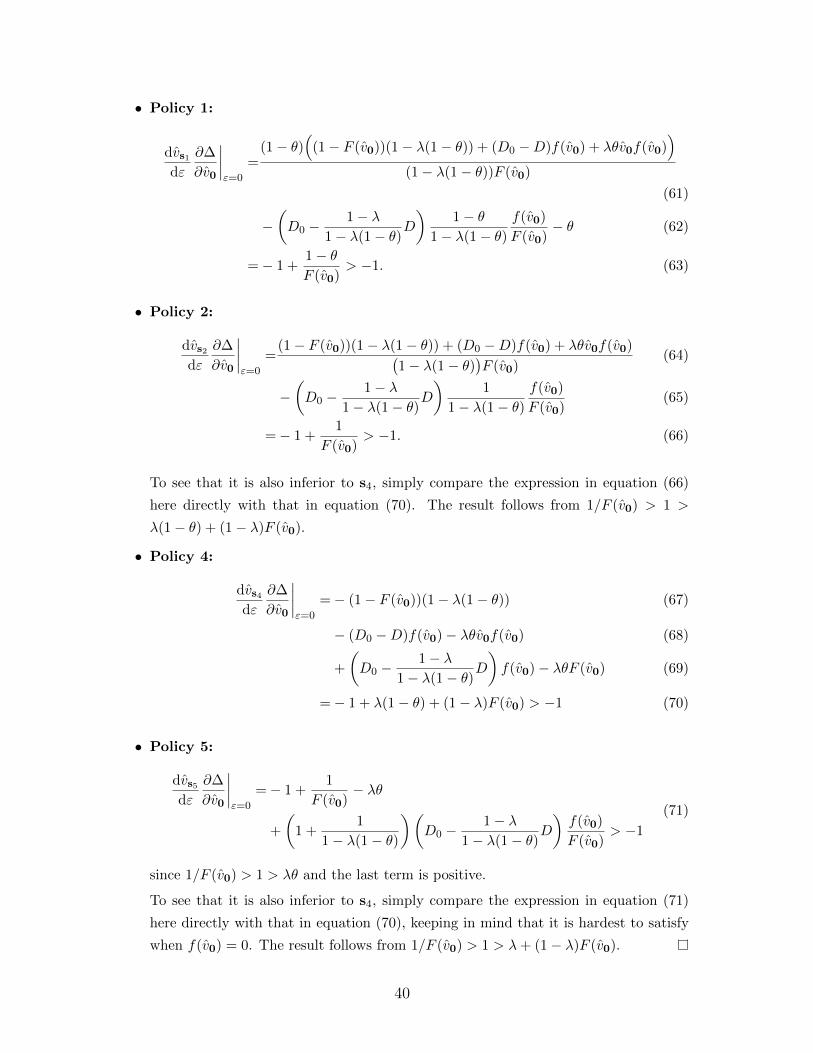
• Policy 1:

dvs1dε

∂∆

∂v0

∣∣∣∣ε=0

=(1− θ)

((1− F (v0))(1− λ(1− θ)) + (D0 −D)f(v0) + λθv0f(v0)

)(1− λ(1− θ))F (v0)

(61)

−(D0 −

1− λ1− λ(1− θ)

D

)1− θ

1− λ(1− θ)f(v0)

F (v0)− θ (62)

=− 1 +1− θF (v0)

> −1. (63)

• Policy 2:

dvs2dε

∂∆

∂v0

∣∣∣∣ε=0

=(1− F (v0))(1− λ(1− θ)) + (D0 −D)f(v0) + λθv0f(v0)(

1− λ(1− θ))F (v0)

(64)

−(D0 −

1− λ1− λ(1− θ)

D

)1

1− λ(1− θ)f(v0)

F (v0)(65)

=− 1 +1

F (v0)> −1. (66)

To see that it is also inferior to s4, simply compare the expression in equation (66)

here directly with that in equation (70). The result follows from 1/F (v0) > 1 >

λ(1− θ) + (1− λ)F (v0).

• Policy 4:

dvs4dε

∂∆

∂v0

∣∣∣∣ε=0

=− (1− F (v0))(1− λ(1− θ)) (67)

− (D0 −D)f(v0)− λθv0f(v0) (68)

+

(D0 −

1− λ1− λ(1− θ)

D

)f(v0)− λθF (v0) (69)

=− 1 + λ(1− θ) + (1− λ)F (v0) > −1 (70)

• Policy 5:

dvs5dε

∂∆

∂v0

∣∣∣∣ε=0

=− 1 +1

F (v0)− λθ

+

(1 +

1

1− λ(1− θ)

)(D0 −

1− λ1− λ(1− θ)

D

)f(v0)

F (v0)> −1

(71)

since 1/F (v0) > 1 > λθ and the last term is positive.

To see that it is also inferior to s4, simply compare the expression in equation (71)

here directly with that in equation (70), keeping in mind that it is hardest to satisfy

when f(v0) = 0. The result follows from 1/F (v0) > 1 > λ+ (1− λ)F (v0).

40

A.9 Proof of Result 9

Note that the result is not quite as immediate as it might seem from equation (42), because

we have to take into account that the equilibrium debt level D∗ and, hence, the default

threshold v = v(D∗) depend on ρ. That said, the immediate intuition does hold: Increasing

ρ increases the write-down. To prove it, we use implicit differentiation.

First, define the difference in a creditor’s payoffs from accepting versus rejecting an offer,

given that other creditors accept:

∆ = (1− F (v))(D −D0) + F (v)E[λθv|v < v]

(1− (1− ρ)

D0

D

)(72)

= (1− F (v))(D −D0) +

(1− (1− ρ)

D0

D

)∫ v

0λθvdF (v). (73)

Now compute the derivative dD∗/dρ in two steps:

∂∆

∂D= (1− F (v)) + (1− ρ)D0D

−2

∫ v

0λθvdF (v)+

+

(D0 −D +

(1− (1− ρ)

D0

D

)λθv

)︸ ︷︷ ︸

=(1−λ+ρλθ)v−(1−λ)v>0

f(v)∂v

∂D> 0

(74)

and∂∆

∂ρ=D0

D

∫ v

0λθvdF (v) > 0. (75)

So,dD∗

dρ= − ∂∆/∂ρ

∂∆/∂D< 0 (76)

and ρ = 1 maximizes the write-down.

A.10 Proof of Result 10

The IC in inequality (43) can be re-written as

∆ = (1− F (v))(D −D0) +

(1− (1− ρ)

D0

D

)λθ

∫ v

0vdF (v) ≥ 0. (77)

The binding IC ∆ = 0 defines the written-down debt level D∗; minimizing D∗ over θ defines

the optimal level of creditor friendliness. Thus, by the chain rule, the effect of ρ on θ∗ is

41

given by:

dθ∗

dρ= −

∂∂ρ

(∂∆∂θ

)∂∂θ

(∂∆∂θ

) = −∂2∆∂ρ∂θ

∂2∆∂θ2

. (78)

Note that the denominator is negative at θ∗ given that we have assumed that θ∗ is an

interior local minimum and not an inflection point.

We compute the denominator directly, step by step:

• First,

∂∆

∂θ=

[f(v)(D0 −D) +

(1− (1− ρ)

D0

D

)λθvf(v)

]∂v

∂θ

+

(1− (1− ρ)

D0

D

)λ

∫ v

0vdF (v)

(79)

=− λvf(v)(v0 − v) +

(1− (1− ρ)

D0

D

)λ

(∫ v

0vdF (v)− λθvf(v)

1− λ(1− θ)v

), (80)

having used that D = (1− λ(1− θ))v, D0 = (1− λ(1− θ))v0, and

∂v

∂θ= − λv

1− λ(1− θ). (81)

• Second,

∂2∆

∂ρ∂θ=D0

Dλ

(∫ v

0vdF (v)− λθvf(v)

1− λ(1− θ)v

). (82)

To determine its sign, it turns out that we can use two facts:

– Using D < D0 in ∆ = 0 above, we get that

1− (1− ρ)D0

D> 0. (83)

– Given θ∗ is optimal, ∂∆/∂θ|θ=θ∗ = 0. This, together with the last inequality,

implies that ∫ v

0vdF (v) >

λθvf(v)

1− λ(1− θ)v. (84)

This implies that ∂2∆/∂ρ∂θ in equation (82) is positive and, thus, given the

above, thatdθ∗

dρ> 0. (85)

42

A.11 Proof of Result 11

The proof is in the text (following the statement of the result).

A.12 Proof of Result 12

Let’s re-write the creditors’ biding IC in equation (18) as a function of η as:

∆ =

∫ ∞v(D)

((1− λη(v)(1− θ))v −D0

)dF η(v) +

∫ v(D)

0θλη(v)vdF η(v) = 0, (86)

having substituted for D = (1− λη(v)(1− θ))v from equation (7).

Solving, we can write the minimum λη(v) needed to restructure to the debt level D as:

λη(v) =

∫∞v(D)(D0 − v)dF η(v)∫ v(D)

0 θvdF η(v)−∫∞v (1− θ)vdF η(v)

(87)

=(D0 − v)(1− F η(v))

θF η(v)Eη[v|v < v]− (1− θ)(1− F η(v))v, (88)

where Eη denotes the expectation given the distribution F η.

Tail expectation Eη[v|v < v] does not depend on η. Given that, by assumption

F η′ � F η, we have that F η

′(v) < F η(v). This implies that the numerator in equation (88)

is increasing in η and the denominator is decreasing in η. Thus, λη′(v) > λη(v).

Default probability F η(v) does not depend on η. That is, F η′(v) = F η(v).

Given that, by assumption F η′ � F η, we have that F η

′(v)Eη

′[v|v < v] > F η(v)Eη[v|v <

v].42 This implies that the denominator of equation (88) is increasing in η. And, since

F η′(v) = F η(v), the numerator is the same under η and η′. Thus, λη

′(v) < λη(v).

42Given F η(v) does not depend on η, this is akin to the fact that F η′ � F η implies Eη

′[v] > Eη[v] and can be

proved via a change of variables, v := (F η)−1(F η

′(v)):

F η(v)Eη[v|v < v] ≡∫ v

0

vdF η(v) =

∫ v

0

(F η)−1(F η

′(v))dF η

((F η)−1

(F η

′(v)))

=

∫ v

0

(F η)−1(F η

′(v))dF η

′(v)

≤∫ v

0

vdF η′(v) ≡ F η

′(v)Eη

′[v|v < v]

where the last inequality follows from the definition of stochastic dominance. That is, F η(v) ≥ F η′(v) or,

equivalently, v ≥ (F η)−1(F η

′(v)). Note, critically, that the assumption that F η(v) does not depend on η allowed

us to change variables without changing the bounds of integration (the result would not obtain without thatassumption).

43

A.13 Proof of Result 13

Here, we solve for the restructuring offer that equity holders make if they face a large,

concentrated creditor (denoted by L in the proof) with probability ξ and small, dispersed

creditors (denoted by S in the proof) with probability 1− ξ.Ultimately, there are three possibilities:

1. The firm makes an offer that L accepts and S reject.

2. The firm makes an offer the L rejects and S accept.

3. The firm makes an offer that both L and S accept.

The proof involves simply (i) computing current equity’s optimal restructuring given

each of these possibilities and (ii) comparing its payoffs (denoted by u in the proof) from

each possibility given these optimal restructurings. But this involves some steps:

Step 1: Write L’s and S’s ICs to accept a restructuring offer.

Step 2: Write current equity’s payoffs u in benchmarks in which ξ = 1 and ξ = 0. That is,

creditors are concentrated for sure or dispersed for sure (these expressions are useful

in the subsequent comparisons).

Step 3: Calculate current equity’s payoffs u for each possibility 1–3 above.

Step 4: Compare these payoffs to determine the optimal restructuring offer.

Step 1: IC constraints. Here, we define the conditions for each type of creditor to

accept the firm’s offer of a restructuring to debt D and equity 1− α.

• Large creditor’s IC. Define the difference in its payoffs from accepting and rejecting

the offer (inequality (47) with the expectations expanded as integrals) as ∆L:

∆L :=

∫ v(D)

0

(θ + (1− θ)(1− α)

)λvf(v)dv +

∫ ∞v(D)

(D + (1− α)(v −D)

)f(v)dv

−∫ v(D0)

0θλvf(v)dv −

∫ ∞v(D0)

D0f(v)dv.

(89)

Its IC is thus ∆L ≥ 0.

• Small creditors’ IC. Define their difference in payoffs from accepting and rejecting the

offer as ∆S :

∆S :=

∫ v(D)

0(θ + (1− θ)(1− α))λvf(v)dv

+

∫ ∞v(D)

(D + (1− α)(v −D))f(v)dv −∫ ∞v(D)

D0f(v)dv.

(90)

44

Their IC is thus ∆S ≥ 0.

Note the difference between these conditions: Whereas L takes into account the effect of

restructuring on the default probability, S do not (this creates the hold-out problem in the

baseline model).

When equity holders make a restructuring offer, they can choose D and 1− α that will

be accepted if there is a large creditor, if there are small creditors, or in both cases. Thus,

they have to take into account which IC is tighter.

Comparing ∆L and ∆S reveals that L’s IC is tighter than S’s if

∆S −∆L =

∫ v(D0)

0λθvf(v)dv −

∫ v(D0)

v(D)D0f(v)dv ≥ 0. (91)

Because this inequality does not depend on α, it is satisfied whenever D is above a threshold,

D, which solves

∆L −∆S

∣∣∣D=D

= 0. (92)

Step 2: Current equity’s payoff u for ξ = 1 and ξ = 0. To find the firm’s payoff,

we define its payoff in the following benchmark cases:

• uL is current equity holders’ payoff if there is a large concentrated creditor (i.e., if

ξ = 1):

uL :=

∫ v(D)

0λvf(v)dv +

∫ ∞v(D)

vf(v)dv −

(∫ v(D0)

0λθvf(v)dv +

∫ ∞v(D0)

D0f(v)dv

).

(93)

• uS is current equity’s payoff if there are small dispersed creditors (i.e., if ξ = 0 as in

the baseline model):

uS :=

∫ v(D)

0λvf(v)dv +

∫ ∞v(D)

vf(v)dv −∫ ∞v(D)

D0f(v)dv. (94)

• u∅ is current equity’s payoff if there is no restructuring (i.e., if D = D0):

u∅ :=

∫ v(D0)

0λ(1− θ)vf(v)dv +

∫ ∞v(D0)

(v −D0)f(v)dv. (95)

These expressions are useful, because equity holders’ payoff for ξ ∈ (0, 1) will be a weighted

average of them.

Step 3: Current equity payoff calculation. There are three possible cases, depend-

ing on which IC binds, which we consider in turn.

Case 1: ∆L ≥ 0 > ∆S. In this case, only L accepts the restructuring but S do not. So

45

the restructuring succeed with probability ξ and equity holders’ problem is to

maximize u = ξuL + (1− ξ)u∅ (96)

over α and D. Given u∅ does not depend on α or D, this is the same as maximizing uL.

Differentiating with respect to D, we find:

−(1− λ)vf(v) < 0, (97)

for all D. So the solution is D = 0. We can find 1− α from the binding IC (∆L = 0):

(1− α)E[v] =

∫ v(D0)

0λθvf(v)dv +

∫ ∞v(D0)

D0f(v)dv. (98)

Defining umaxL as the maximum of uL in this case, we have:

umaxL =

∫ ∞0

vf(v)dv −

(∫ v(D0)

0λθvf(v)dv +

∫ ∞v(D0)

D0f(v)dv

). (99)

So the expected payoff is:

u = ξumaxL + (1− ξ)u∅. (100)

Case 2: ∆S ≥ 0 > ∆L. In this case, only the small creditors’ IC is satisfied. So the

restructuring succeed with probability 1− ξ and and equity holders’ problem is to

maximize u = ξu∅ + (1− ξ)uS (101)

over α and D. Given u∅ does not depend on α or D, this is the same as maximizing

uS . This is the baseline case of dispersed creditors studied in Section B.1: 1 − α = 0 and

D = D∗.

Defining umaxS as the maximum of uS in this case, we have:

umaxS =

∫ v(D)

0λvf(v)dv +

∫ ∞v(D)

vf(v)dv −∫ ∞v(D)

D0f(v)dv. (102)

So the expected payoff is

u = ξu∅ + (1− ξ)umaxS . (103)

Case 3: ∆S ≥ 0 and ∆L ≥ 0. In this case, both ICs are satisfied and equity holders’

problem is to

maximize u = ξuL + (1− ξ)uS (104)

over α and D.

46

Here, there are three sub-cases:

• Case 3(i): ∆L > ∆S = 0 ( =⇒ D < D). In this case, the firm chooses α and D so

that S’s IC binds and L accepts the restructuring on S’s terms. Hence, the equity

holders problem is to

maximize u = ξuS + (1− ξ)uS = uS (105)

over α and D. From case 2, we know that to maximize uS , equity holders set 1−α = 0

and D = D∗. So the expected payoff is:

u = umaxS . (106)

• Case 3(ii): ∆S > ∆L = 0 ( =⇒ D > D). This cannot arise in equilibrium: Given S’s

IC is slack (∆S > 0), equity holders can increase their surplus by decreasing D (and

increasing 1− α so as not to violate L’s IC).

• Case 3(iii): ∆S = ∆L = 0 ( =⇒ D = D). Given both ICs are binding, D = D by

definition. Here, the expected payoff is:

u = uS(D) = uL(D). (107)

In this case, the offer includes both debt D and an equity stake 1− α, which we can

solve for from the binding ICs:

1− α =

∫ vD00 λθvf(v)dv +

∫∞v(D0)D0f(v)dv −

∫ v(D)0 θλvf(v)dv −

∫∞v(D) Df(v)dv∫ v(D)

0 (1− θ)λvf(v)dv +∫∞v(D)(v − D)f(v)dv

.

(108)

Combining these sub-cases, we have that equity’s expected payoff is:

u =

umaxS if D∗ < D,

uS(D) if D∗ ≥ D.(109)

Step 4: Payoff comparison. Combining the cases above, we have that equity’s

expected payoff is:

u =

max

{ξumax

L + (1− ξ)u∅ , ξu∅ + (1− ξ)umaxS , umax

S

}if D∗ < D,

max{ξumax

L + (1− ξ)u∅ , ξu∅ + (1− ξ)umaxS , uS(D)

}if D∗ ≥ D.

(110)

To simplify the thresholds above, first observe that, from the definitions of umaxL , umax

S ,

47

and uS(D) and the assumption that D0 is sufficiently large (and hence u∅ sufficiently small),

we have:

umaxL ≥ uL(D) = uS(D) > u∅ (111)

and

umaxS ≥ uL(D) = uS(D) > u∅. (112)

With this, we can re-write u as:

u =

max

{ξumax

L + (1− ξ)u∅ , umaxS

}if D∗ < D

max{ξumax

L + (1− ξ)u∅ , ξu∅ + (1− ξ)umaxS , uS(D)

}if D∗ ≥ D.

(113)

To give the formulation in the statement of the result, we divide the expression above

into cases for D∗ ≶ D and ξ ≶ ξ, where:

ξ :=umaxS − uS(D)

umaxS − u∅

, (114)

ξ :=uS(D)− u∅umaxL − u∅

. (115)

• If D∗ ≥ D and ξ < ξ, then:

u =

ξu∅ + (1− ξ)umax

S if ξ ≤ ξ,

uS(D) if ξ ∈(ξ, ξ],

ξumaxL + (1− ξ)u∅ if ξ > ξ

(116)

The analysis above implies this corresponds to debt for ξ ≤ ξ, a mix of debt and

equity for ξ ∈ (ξ, ξ], and equity for ξ > ξ.

• If D∗ ≥ D and ξ ≥ ξ, then:

u =

ξu∅ + (1− ξ)umax

S if ξ ≤umaxS − u∅

umaxL + umax

S − 2u∅,

ξumaxL + (1− ξ)u∅ if ξ >

umaxS − u∅

umaxL + umax

S − 2u∅.

(117)

The analysis above implies this corresponds to debt for ξ below the threshold (umaxS −

u∅)/(umaxL + umax

S − 2u∅) and equity above it.

48

• If D∗ < D, then:

u =

umaxS if ξ ≤ umax

S −u∅umaxL −u∅

ξumaxL + (1− ξ)u∅ if ξ >

umaxS −u∅umaxL −u∅ .

(118)

The analysis above implies this corresponds to debt for ξ below the threshold (umaxS −

u∅)/(umaxL − u∅) and equity above it.

B Omitted Derivations

B.1 Mixed Offers

In our baseline model, we study exchange offers including a single security, equity or debt. In

Section 5.4, we show that offers of a mix and debt and equity could arise with a concentrated

creditor. Here, we show they never arise in our baseline model with dispersed creditors.

Suppose that the firm offers creditors a mix of a proportion of equity 1− α and senior

debt with face value D in exchange for their junior debt D0.

Noting that the bankruptcy decision condition in equation (7) is unchanged by new

equity (i.e., that the firm will file whenever v ≤ v(D)), we can write a creditor’s payoffs as

follows:

• If it accepts, it gets:

payoff∣∣acc.

=(1− F (v)

)D +

∫ v

0(θ + (1− α)(1− θ))λvdF (v)

+

∫ ∞v

(1− α)(v −D)dF (v).

(119)

• If it rejects, it gets:

payoff∣∣rej.

=(1− F (v)

)D0. (120)

So the firm chooses α and D to

maximize

∫ v

0αλ(1− θ)vf(v)dv +

∫ ∞v

α(v −D)f(v)dv (121)

subject to creditors’ IC that

payoff∣∣acc.≥ payoff

∣∣rej.

(122)

Supposing that the constraint binds and substituting it in the objective, we can re-write

49

the problem as:

maximize

∫ v

0λvdF (v) +

∫ v

vvdF (v)− (1− F (v(D)))D0. (123)

Now observe that this does not depend on α and that D appears only in v. Hence, if there

is an interior optimum, we can maximize the objective with respect to v directly, to get:

−λf(v)v + f(v)v + f(v)D0 = 0. (124)

Substituting in for v from equation (7) and solving, we find that:

D =1− λ(1− θ)

1− λD0 > D0. (125)

Still supposing an interior optimum, substitute D0 into the binding constraint in (122) to

get that:

(1− α)

(∫ v

0+(1− θ)λvdF (v) +

∫ ∞v

(v −D)dF (v)

)=

= −(1− F (v)

))θλv(D)−

∫ v

0θλvdF (v).

(126)

But this implies that new equity is negative. So we conclude that there is not an interior

optimum, but, rather, that 1− α = 0. Substituting into the constraint (122), we get:

(1− F (v))D +

∫ v

0θλvf(v)dv ≥ (1− F (v))D0, (127)

which is the usual constraint.

B.2 Omitted derivation from Section 3.8

Given equations (52) and (53), inequality (30) is equivalent to:

∂∆

∂θ= λ

∫ v

0vdF (v) +

(λθv +D0 −D∗

)f(v)

∂v

∂θ< 0. (128)

50

To massage this expression, we re-write ∂v/∂θ using equation (7) as follows:

∂v

∂θ= − λD

(1− (1− θ)λ)2 (129)

= −λ D

1− (1− θ)λ1

1− (1− θ)λ(130)

= −λv ∂v∂D

. (131)

With this, inequality (128) becomes:

1

v

∫ v

0vdF (v) < λθv

∂F (v)

∂D+ (D0 −D)

∂F (v)

∂D. (132)

Observe that the left-hand side is less than one43 and that the second term on the

right-hand side is positive, so we can write a sufficient condition:

1 < λθv∂F (v)

∂D. (133)

This is the condition in the text.

B.3 Omitted Derivations from Section 4

We compute the marginal effect of a dollar for each policy si, as in equation (40). To

streamline some of the calculations, we change variables, and write things in terms of the

default threshold in the baseline model v0 instead of the debt level D. Since v0 ∝ D

(equation (7)), equation (40) can be re-written as:

dvsidε

∣∣∣∣ε=0

=

(∂vsi∂si− ∂vsi∂v0

∂∆/∂si∂∆/∂v0

)1

q i. (134)

We go through the omitted steps for each policy in turn:

Policy 1: Bankruptcy Subsidies for Assets.

• Cost: s1 is paid conditional on bankruptcy and bankruptcy occurs with probability

F (vs1), so q1 = F (vs1).

• Filing: s1 increases the firm’s asset value in bankruptcy, so, given equation (5), the

firm files if

(1− θ) (λv + s1) ≥ v −D, (135)

43The average of v given v ≤ v is less than v.

51

giving filing threshold

vs1 :=D + (1− θ)s1

1− λ(1− θ)≡ v0 +

(1− θ)s1

1− λ(1− θ). (136)

From equation (136)

∂vs1∂v0

= 1 and∂vs1∂s1

=1− θ

1− λ(1− θ). (137)

• Restructuring: The binding IC is:

∆ =(1− F (vs1)

)(D −D0) +

∫ vs1

0θ (λv + s1) dF (v) = 0, (138)

where the subsidy affects both the probability that the creditors are repaid in full (via

vs1) and what they get if they are not (because they share s1).

We differentiate ∆ in equation (138) w.r.t. s1 and v0:

∂∆

∂s1= −f(vs1)(D −D0)

∂vs1∂s1

+

∫ vs1

0θdF (v) + θ(λvs1 + s1)f(vs1)

∂vs1∂s1

(139)

→(D0 −

1− λ1− λ(1− θ)

D

)1− θ

1− λ(1− θ)f(v0) + θF (v0), (140)

as ε→ 0, given vs1 = v0 when ε = 0.

And

∂∆

∂v0=(1− F (vs1)

)∂D∂v− (D −D0)f(vs1) + λθ(vs1 + s1)f(vs1)

∂vs1∂v

(141)

→ (1− F (v0))(1− λ(1− θ)) + (D0 −D)f(v0) + λθv0f(v0), (142)

as ε→ 0.

Substituting the above and q1 = F (v0) into equation (134), we find the marginal benefit

of investing in policy s1:

dvs1dε

∣∣∣∣ε=0

=

1− θ1− λ(1− θ)

−

(D0 − 1−λ

1−λ(1−θ)D)

1−θ1−λ(1−θ)f(v0) + θF (v0)

(1− F (v0))(1− λ(1− θ)) + (D0 −D)f(v0) + λθv0f(v0)

1

F (v0).

(143)

Policy 2: Bankruptcy Subsidies for Equity.

• Cost: s2 is paid conditional on bankruptcy, and bankruptcy occurs with probability

F (vs2), so q2 = F (vs2).

52

• Filing: s2 increases equity holders’ payoff in bankruptcy, so, given equation (5), the

firm files if

(1− θ)λv + s2 ≥ v −D, (144)

giving the filing threshold

vs2 := v0 +s2

1− λ(1− θ). (145)

From equation (145), we have:

∂vs2∂v0

= 1 and∂vs2∂s2

=1

1− λ(1− θ). (146)

• Restructuring: The binding IC is

∆ =(1− F (vs2)

)(D −D0) +

∫ vs2

0λθvdF (v), (147)

where the subsidy affects the probability that the creditors are repaid in full (via vs2),

but does not affect what they receive if they are not paid in full (because the subsidy

goes entirely to equity).

We differentiate ∆ in equation (147) with respect to s2 and v0:

∂∆

∂s2= −f(vs4)(D −D0)

∂vs2∂s2

+ λθvs2f(vs2)∂vs2∂s2

(148)

→(D0 −

1− λ1− λ(1− θ)D

)1

1− λ(1− θ)f(v0), (149)

as ε→ 0, given vs2 → v0 as ε→ 0.

And

∂∆

∂v0=(1− F (vs2)

) ∂D∂v0− f(vs2)(D −D0) + λθvs2f(vs2)

∂vs2∂v0

(150)

→(1− F (v0)

)(1− λ(1− θ)

)+ (D0 −D)f(v0) + λθv0f(v0), (151)

as ε→ 0.

Substituting the above and q2 = F (v0) into equation (134) above, we can find the

marginal benefit of investing in policy s2:

dvs2dε

∣∣∣ε=0

=

1

1− λ(1− θ)−

(D0 − 1−λ

1−λ(1−θ)D

)1

1−λ(1−θ)f(v0)

(1− F (v0))(1− λ(1− θ)) + (D0 −D)f(v0) + λθv0f(v0)

1

F (v0).

(152)

Policy 3: Bankruptcy Subsidies for Debt.

53

• Cost: s3 is paid conditional on bankruptcy and bankruptcy occurs with probability

F (vs3), so q3 = F (vs3).

• Filing: s3 does not affect equity holders’ payoffs (only creditors’). Hence, vs3 = v0.

Thus, we have:∂vs3∂v0

= 1 and∂vs3∂s3

= 0. (153)

• Restructuring: The binding IC is:

∆ =(1− F (vs3)

)(D −D0) +

∫ vs3

0(λθv + s3) dF (v) = 0, (154)

where the subsidy affects both the probability that the creditors are repaid (via vs3)

and what they get if they are not repaid in full (because they get s3).

We differentiate ∆ in equation (154) with respect to s3 and v0:

∂∆

∂s3= F (v0). (155)

And,

∂∆

∂v0=(1− F (v0)

)(1− λ(1− θ)

)+ (D0 −D)f(v0) + λθv0f(v0). (156)

Substituting the above and q3 = F (v0) into equation (134) above, we can find the

marginal benefit of investing in policy s3:

dvs3dε

∣∣∣∣ε=0

= − 1

(1− F (v))(1− λ(1− θ)) + (D0 −D)f(v) + λθvf(v). (157)

Policy 4: Asset Subsidies.

• Cost: s4 is paid unconditionally, so q4 = 1.

• Filing: s4 increases the firm’s asset value in the firm’s payoff (equation (5)), giving

the filing threshold

vs4 :=D

1− (1− θ)λ− s4 ≡ v0 − s4, (158)

where v0 denotes the filing threshold in the baseline model with no policy intervention,

as given in equation (7).

From equation (158), we have:

∂vs4∂v0

= 1 and∂vs4∂s4

= −1. (159)

54

• Restructuring: The binding IC is:

∆ =(1− F (vs4)

)(D −D0) +

∫ vs4

0λθ(v + s4)dF (v) = 0, (160)

where the subsidy affects both the probability that the creditors are repaid in full (via

vs4) and what they get if they are not repaid in full (because they share s4).44

We differentiate the ∆ in equation (160) with respect to s4 and v0:

∂∆

∂s4= −f(vs4)(D −D0)

∂vs4∂s4

+

∫ vs4

0λθdF (v) + λθ(vs4 + s4)f(vs4)

∂vs4∂s4

(161)

→ −(D0 −

1− λ1− λ(1− θ)

D

)f(v0) + λθF (v0), (162)

as ε→ 0, given vs4 → v0 as ε→ 0.

And,

∂∆

∂v0=(1− F (vs4)

) ∂D∂v0− f(vs4)(D −D0) + λθ(vs4 + s4)f(vs4)

∂vs4∂v0

(163)

→(1− F (v0)

)(1− λ(1− θ)

)+ (D0 −D)f(v0) + λθv0f(v0), (164)

as ε→ 0.

Substituting the above and q4 = 1 into equation (134) above, we can find the marginal

benefit of investing in policy s4:

dvs4dε

∣∣∣∣ε=0

= −1 +

(D0 − 1−λ

1−λ(1−θ)D)f(v0)− λθF (v0)

(1− F (v0))(1− λ(1− θ)) + (D0 −D)f(v0) + λθv0f(v0). (165)

Policy 5: Subsidized Lending.

• Cost: s5 is paid unconditionally and repaid conditional on solvency, which occurs

with probability 1 − F (vs5) (it is not repaid in bankruptcy, since it is diluted in

restructuring). Thus,

q5 = 1−(1− F (vs5)

)= F (vs5). (166)

• Filing: s5 increases both the firm’s assets and liabilities in the firm’s payoff (equation

(5)), giving the filing threshold

vs5 :=D

1− (1− θ)λ+

s5

1− (1− θ)λ≡ v0 +

s5

1− (1− θ)λ. (167)

44Note that the lower bound on the integral is 0 (instead of −s4) because f = 0 on [−s4, 0).

55

From equation (167), we have:

∂vs5∂v0

= 1 and∂vs5∂s5

=1

1− λ(1− θ). (168)

• Restructuring: The binding IC is:

∆ =(1− F (vs5)

)(D −D0) +

∫ vs5

0λθ(v + s5)dF (v) = 0, (169)

where the subsidy affects both the probability that the creditors are repaid in full (via

vs5) and what they get if they are not repaid in full (because they share s5).

We differentiate ∆ in equation (169) with respect to s5 and v0:

∂∆

∂s5= −f(vs5)(D −D0)

∂vs5∂s5

+

∫ vs5

0λθdF (v) + λθ(vs5 + s5)f(vs5)

∂vs5∂s5

(170)

→ −(D0 −

1− λ1− λ(1− θ)

D

)f(v0) + λθF (v0), (171)

as ε→ 0, given vs5 → v0 as ε→ 0.

And,

∂∆

∂v0=(1− F (vs5)

) ∂D∂v0− f(vs5)(D −D0) + λθ(vs5 + s5)f(vs5)

∂vs5∂v0

(172)

→(1− F (v0)

)(1− λ(1− θ)

)+ (D0 −D)f(v0) + λθv0f(v0), (173)

as ε→ 0.

Substituting the above and q5 = F (v0) into equation (134) above, we can find the

marginal benefit of investing in policy s5:

dvs5dε

∣∣∣∣ε=0

=

1

1− λ(1− θ)+

(D0 − 1−λ

1−λ(1−θ)D)f(v0)− λθF (v0)

(1− F (v0))(1− λ(1− θ)) + (D0 −D)f(v0) + λθv0f(v0)

1

F (v0).

(174)

Policy 6: Debt Purchases (and Forgiveness).

• Cost: The cost is the market price of debt, which, given debt holders take into account

the debt reduction and future restructuring, is just q6 = 1− F (vs6).

• Filing: s6 does not affect equity holder’s payoffs directly. Hence, vs6 = v0. Thus, we

have:∂vs6∂v

= 1 and∂vs6∂s6

= 0. (175)

• Restructuring: The binding IC is:

56

∆ =(1− F (vs6)

)(D − (D0 − s6)

)+

∫ vs6

0λθvdF (v), (176)

where the subsidy affects the probability that the creditors are repaid in full (via vs6)

and what they get if they hold out (because s6 reduces the face value).

We differentiate ∆ in equation (154) with respect to s3 and v0:

∂∆

∂s6= 1− F (v0). (177)

And,

∂∆

∂v0=(1− F (v0)

)(1− λ(1− θ)

)+ (D0 −D)f(v0) + λθv0f(v0). (178)

Substituting the above and q6 = 1 − F (v0) into equation (134) above, we can find the

marginal benefit of investing in policy s6. We get the same for policy s3 (equation (157)):

dvs6dε

∣∣∣∣ε=0

=dvs3dε

∣∣∣∣ε=0

. (179)

Policy 7: Restructuring Subsidies.

• Cost: s7 is paid conditional on a restructuring, but restructuring occurs with proba-

bility one in equilibrium, so q7 = 1.

• Filing: s7 does not affect equity holders’ payoffs directly. Hence, vs7 = v0. Thus, we

have:∂vs7∂v0

= 1 and∂vs7∂s7

= 0 (180)

• Restructuring: The binding IC is:

∆ = s7 +(1− F (v0)

)(D −D0) +

∫ v0

0λθvdF (v) = 0, (181)

where the subsidy does not affect the probability that the creditors are repaid (because

vs7 = v0) but only affects what they get if they accept the restructuring (because they

get s7).

We differentiate ∆ in equation (181) with respect to s7 and v0:

∂∆

∂s7≡ 1. (182)

And

∂∆

∂v0=(1− F (v0)

)(1− λ(1− θ)

)+ (D0 −D)f(v0) + λθv0f(v0). (183)

57

Substituting the above and q7 = 1 into equation (134) above, we find the marginal

benefit of investing in policy s7 is the same as for policies s3 and s6:

dvs7dε

∣∣∣∣ε=0

=dvs3dε

∣∣∣∣ε=0

=dvs6dε

∣∣∣∣ε=0

. (184)

B.4 What if Powerful Secured Creditors Destroy Value for

Equity Holders?

Here, we assume that for creditors to gain $1 in bankruptcy, equity holders must forgo more

than $1. Specifically, for every (1 − γ/2)θλv that creditors get, equity gives up (1 − θ)λv.Thus, γ measures the inefficiencies they induce ex post. If γ = 0, the model is the same as

the baseline. Increasing γ decreases the total surplus.

To explore how the inefficiencies of creditor power could affect restructuring, we explore

how the optimal level of creditor friendliness depends on the inefficiencies induced by secured

creditor power γ (cf. Section 3.7 and Section 3.8). This gives the next result:

Result 14. Suppose that the write-down is maximized at a unique interior level of creditor

friendliness θ∗ that is not an inflection point (as in, e.g., the uniform case in Figure 1).

Increasing the inefficiency of secured creditor power γ decreases the optimal level of creditor

friendliness. That is, dθ∗/dγ < 0.

Intuitively, if giving creditors power destroys value in bankruptcy, then giving them more

power is likely to make them even less willing to accept a restructuring. Hence, the larger

is γ, the larger is the region of θ for which making the code more creditor friendly makes

restructuring harder.

Proof. We begin from the creditors’ IC:

∆ = (1− F (v))(D −D0) + λθ

(1− γθ

2

)∫ v

0vdF (v), (185)

which is just the creditors’ IC in equation (26) modified to include the inefficiencies captured

by γ . The binding IC, ∆ = 0, defines the written-down debt level D∗ and minimizing D∗

over θ defines the optimal level of creditor friendliness θ∗. Thus, by the chain rule, the

effect of γ on θ∗ is given by:

dθ∗

dγ= −

∂∂γ

(∂∆∂θ

)∂∂θ

(∂∆∂θ

) = −∂2∆/(∂γ∂θ)

∂2∆/∂θ2. (186)

Note that the denominator is negative given that we have assumed that θ∗ is an interior

local minimum and not an inflection point.

We compute the numerator ∂2∆∂γ∂θ directly, step by step:

58

• First,

∂∆

∂θ=λ (1− γθ)

∫ v

0vdF (v) +

[D0 −D + λθ

(1− γθ

2

)v

]f(v)

∂v

∂θ(187)

=λ (1− γθ)∫ v

0vdF (v)− λ

[v0 − v +

λθ (2− γθ)2(1− λ(1− θ))

v

]vf(v), (188)

having used that D = (1− λ(1− θ))v, D0 = (1− λ(1− θ))v0, and

∂v

∂θ=

−λv1− λ(1− θ)

. (189)

• Second,

∂2∆

∂γ∂θ=− λθ

(∫ v

0vdF (v)− λθ

2(1− λ(1− θ))v2f(v)

). (190)

To determine the sign, it turns out that we can we can use the fact that θ∗ is optimal,

so ∂∆/∂θ|θ=θ∗ = 0. That is, the derivative in equation (188) is zero. Manipulating, we get:

λ (1− γθ)(∫ v

0vdF (v)− λθ

2(1− λ(1− θ))v2f(v)

)−λ[v0 − v +

λθ

2(1− λ(1− θ))v

]vf(v) = 0

(191)

and, thus, that:

−∫ v

0vdF (v) +

λθ

2(1− λ(1− θ))v2f(v) = − (1− γθ)−1

[v0 − v +

λθ

2(1− λ(1− θ))v

]vf(v),

(192)

which is the numerator in equation (190). It is negative given that v0 > v.

Substituting into equation (186), we see that dθ∗/dγ is negative.

59

References

Adler, B. E. (1995). A re-examination of near-bankruptcy investment incentives. University

of Chicago Law Review 62 (2), 575–606.

Adler, B. E., V. Capkun, and L. A. Weiss. Value destruction in the new era of chapter 11.

Aghion, P. and P. Bolton (1992). An incomplete contracts approach to financial contracting.

Review of Economic Studies 59 (3), 473–494.

Antill, S. (2020). Do the right firms survive bankruptcy? Working paper, Harvard Business

School.

Asquith, P., R. Gertner, and D. Scharfstein (1994). Anatomy of financial distress: An

examination of junk-bond issuers. Quarterly Journal of Economics 109 (3), 625–658.

Ayotte, K. and J. Ellias (2020). Bankruptcy process for sale. Research paper no. 382,

UC–Hastings.

Ayotte, K. and H. Yun (2009). Matching bankruptcy law to legal environments. Journal

of Law, Economics, & Organization 25 (1), 2–30.

Ayotte, K. M. and E. R. Morrison (2009). Creditor control and conflict in chapter 11.

Journal of Legal Analysis 1 (2), 511–551.

Bagnoli, M. and B. L. Lipman (1988). Successful takeovers without exclusion. Review of

Financial Studies 1 (1), 89–110.

Baird, D. (1986). The uneasy case for corporate reorganizations. Journal of Legal Stud-

ies 15 (1), 127–147.

Baird, D. G. (1991). The initiation problem in bankruptcy. International Review of Law

and Economics 11 (2), 223 – 232.

Bebchuk, L. A. (2002). Ex ante costs of violating absolute priority in bankruptcy. Journal

of Finance 57 (1), 445–460.

Bebchuk, L. A. and J. M. Fried (1996). The uneasy case for the priority of secured claims

in bankruptcy. Yale Law Journal 105 (4), 857–934.

Becker, B. and J. Josephson (2016). Insolvency resolution and the missing high-yield bond

markets. Review of Financial Studies 29 (10), 2814–2849.

Benmelech, E., N. Kumar, and R. Rajan (2020). Secured credit spreads. Working paper,

Northwestern University.

60

Bernardo, A. E. and E. L. Talley (1996). Investment policy and exit-exchange offers within

financially distressed firms. Journal of Finance 51 (3), 871–888.

Bernstein, S., E. Colonnelli, and B. Iverson (2019). Asset allocation in bankruptcy. Journal

of Finance 74 (1), 5–53.

Bisin, A. and A. A. Rampini (2005). Exclusive contracts and the institution of bankruptcy.

Economic Theory 27 (2), 277–304.

Bjerre, C. S. (1999). Secured transactions inside out: Negative pledge covenants, property

and perfection. Cornell Law Review 84 (2).

Blanchard, O., T. Philippon, and J. Pisani-Ferry (2020). A new policy toolkit is needed

as countries exit COVID-19 lockdowns. Peterson Institute for International Economics

Policy Brief 20-8, 1–19.

Bris, A., I. Welch, and N. Zhu (2006). The costs of bankruptcy: Chapter 7 liquidation

versus Chapter 11 reorganization. Journal of Finance 61 (3), 1253–1303.

Brunnermeier, M. and A. Krishnamurthy (2020). Corporate debt overhang and credit

policy. BPEA Conference Drafts, Brookings Papers on Economic Activity.

Bulow, J. I. and J. B. Shoven (1978). The bankruptcy decision. Bell Journal of Eco-

nomics 9 (2), 437–456.

Campbell, J. Y., J. Hilscher, and J. Szilagyi (2008). In search of distress risk. Journal of

Finance 63 (6), 2899–2939.

Campello, M., T. Ladika, and R. Matta (2018). Renegotiation frictions and financial distress

resolution: Evidence from cds spreads. Review of Finance 23 (3), 513–556.

Casey, A. J. (2011). The creditors’ bargain and option-preservation priority in chapter 11.

University of Chicago Law Review 78, 759–807.

Chaney, T., D. Sraer, and D. Thesmar (2012). The collateral channel: How real estate

shocks affect corporate investment. American Economic Review 102 (6), 2381–2409.

Chatterjee, S., U. S. Dhillon, and G. G. Ramarez (1995). Coercive tender and exchange

offers in distressed high-yield debt restructurings an empirical analysis. Journal of Fi-

nancial Economics 38 (3), 333–360.

Colla, P., F. Ippolito, and K. Li (2020). Debt structure. Journal of Law, Economics, &

Organization 12 (1).

61

Davydenko, S. A., I. A. Strebulaev, and X. Zhao (2012). A market-based study of the cost

of default. Review of Financial Studies 25 (10), 2959–2999.

DeMarzo, P., A. Krishnamurthy, and J. Rauh (2020). Debtor-in-possession financing facility

(DIPFF) proposal. Working paper, Stanford GSB.

Diamond, D. W. (1993). Seniority and maturity of debt contracts. Journal of Financial

Economics 33 (3), 341–368.

Donaldson, J. R., D. Gromb, and G. Piacentino (2020a). Conflicting priorities: A theory

of covenants and collateral. Working paper, Washington University in St. Louis.

Donaldson, J. R., D. Gromb, and G. Piacentino (2020b). The paradox of pledgeability.

Journal of Financial Economics 137 (3), 591–605.

Donaldson, J. R. and G. Piacentino (2020). Netting. Working paper, Washington University

in St. Louis.

Dou, W. W., L. A. Taylor, W. Wang, and W. Wang (2020). Dissecting bankruptcy frictions.

Working paper, Jacobs Levy Equity Management Center for Quantitative Financial Re-

search, The Wharton School.

Eberhart, A., W. Moore, and R. Roenfeldt (1990). Security pricing and deviations from the

absolute priority rule in bankruptcy proceedings. Journal of Finance 45 (5), 1457–1469.

Eckbo, E., K. Li, and W. Wang (2019). Rent extraction by super-priority lenders. Working

paper, Tuck School of Business.

Fan, H. and S. Sundaresan (2000). Debt valuation, renegotiation, and optimal dividend

policy. Review of Financial Studies 13 (4), 1057–1099.

Favara, G., E. Schroth, and P. Valta (2012). Strategic default and equity risk across coun-

tries. Journal of Finance 67 (6), 2051–2095.

Franks, J. and W. Torous (1989). An empirical investigation of U.S. firms in reorganization.

Journal of Finance 44 (3), 747–769.

Franks, J. R. and W. N. Torous (1994). A comparison of financial recontracting in distressed

exchanges and Chapter 11 reorganizations. Journal of Financial Economics 35 (3), 349–

370.

Gelman, A. and J. Hill (2007). Data analysis using regression and multilevel/hierarchical

models. New York, NY: Cambridge University Press.

62

Gertner, R. and D. Scharfstein (1991). A theory of workouts and the effects of reorganization

law. Journal of Finance 46 (4), 1189–1222.

Giambona, E., F. Lopez-de Silanes, and R. Matta (2019). Stiffing the creditor: The effect

of asset verifiability on bankruptcy. Working paper, Syracuse University.

Giammarino, R. (1989). The resolution of financial distress. Review of Financial Stud-

ies 2 (1), 25–47.

Gilson, S. C., K. John, and L. H. Lang (1990). Troubled debt restructurings: An empirical

study of private reorganization of firms in default. Journal of Financial Economics 27 (2),

315–353.

Greenwood, R. and D. Thesmar (2020). Sharing the economic pain of the coronavirus.

Working paper, Harvard Business School.

Grossman, S. J. and O. D. Hart (1980). Takeover bids, the free-rider problem, and the

theory of the corporation. Bell Journal of Economics 11 (1), 42–64.

Hart, O. (1995). Firms, Contracts, and Financial Structure. Oxford University Press.

Hart, O. and J. Moore (1994, November). A theory of debt based on the inalienability of

human capital. Quarterly Journal of Economics 109 (4), 841–79.

Hart, O. and J. Moore (1995). Debt and seniority: An analysis of the role of hard claims

in constraining management. American Economic Review 85 (3), 567–85.

Hart, O. and J. Moore (1998). Default and renegotiation: A dynamic model of debt.

Quarterly Journal of Economics 113 (1), 1–41.

Haugen, R. A. and L. W. Senbet (1978). The insignificance of bankruptcy costs to the

theory of optimal capital structure. Journal of Finance 33 (2), 383–393.

Haugen, R. A. and L. W. Senbet (1988). Bankruptcy and agency costs: Their signifi-

cance to the theory of optimal capital structure. Journal of Financial and Quantitative

Analysis 23 (1), 27–38.

Holmstrom, B. and J. Tirole (1997). Financial Intermediation, Loanable Funds, and the

Real Sector. Quarterly Journal of Economics 112 (3), 663–91.

Hotchkiss, E. S., K. John, R. M. Mooradian, and K. S. Thorburn (2008). Chapter 14 –

Bankruptcy and the resolution of financial distress. In B. E. Eckbo (Ed.), Handbook of

Empirical Corporate Finance, pp. 235–287. San Diego: Elsevier.

63

Hynes, R. and S. Walt (2020). Revitalizing involuntary bankruptcy. Iowa Law Review 105,

1127–1185.

Iverson, B. (2018). Get in line: Chapter 11 restructuring in crowded bankruptcy courts.

Management Science 64 (11), 4967–5460.

Iverson, B., J. Ellias, and M. Roe (2020). Estimating the need for additional bankruptcy

judges in light of the COVID-19 pandemic. Harvard Business Law Review, forthcoming.

Jacoby, M. B. and E. J. Janger (2014). Ice cube bonds: Allocating the price of process in

Chapter 11 bankruptcy. Yale Law Journal 123, 862–1117.

James, C. (1995). When do banks take equity in debt restructurings? Review of Financial

Studies 8 (4), 1209–1234.

Jensen, M. C. (1986). Agency costs of free cash flow, corporate finance, and takeovers.

American Economic Review 76 (2), 323–329.

Jiang, W., K. Li, and W. Wang (2012). Hedge funds and chapter 11. Journal of Fi-

nance 67 (2), 513–560.

Jostarndt, P. and Z. Sautner (2009, 11). Out-of-court restructuring versus formal

bankruptcy in a non-interventionist bankruptcy setting. Review of Finance 14 (4), 623–

668.

Kahan, M. and B. Tuckman (1993). Do bondholders lose from junk bond covenant changes.

Journal of Business 66 (4), 499–516.

Leland, H. E. (1994). Corporate debt value, bond covenants, and optimal capital structure.

Journal of Finance 49 (4), 1213–1252.

Levin, R. and H. J. Sommer (Eds.) (2020). Collier on Bankruptcy (16th ed.). New Provi-

dence, NJ: LexisNexis.

Miller, H. and R. Berkovich (2006). The implications of the Third Circuit’s Armstrong deci-

sion on creative corporate restructuring: Will strict construction of the Absolute Priority

Rule make Chapter 11 consensus less likely? American University Law Review 55 (5),

1345–1426.

Moody’s (2017). A closer look at distressed exchanges. Data Report, 19 December 2017.

Moody’s (2020). Recoveries in a pandemic-driven default cycle. Sector In-Depth Report,

20 May 2020.

64

Mooradian, R. and H. Ryan (2005). Out-of-court restructurings and the resolution of

financial distress: Section 3(a)(9) compared to investment-bank-managed exchange offers.

Journal of Business 78 (4), 1593–1624.

Mooradian, R. M. (1994). The effect of bankruptcy protection on investment: Chapter 11

as a screening device. Journal of Finance 49 (4), 1403–1430.

Morrison, E. R. and A. C. Saavedra (2020). Bankruptcy’s role in the COVID-19 crisis. In

K. Pistor (Ed.), Law in the Time of COVID-19, pp. 127–140. New York, NY: Columbia

Law School.

Myers, S. C. (1977). Determinants of corporate borrowing. Journal of Financial Eco-

nomics 5 (2), 147–175.

Picker, R. C. (1992). Voluntary petitions and the creditors’ bargain. Cincinnati Law

Review 61, 519–541.

Povel, P. (1999). Optimal “soft” or “tough” bankruptcy procedures. Journal of Law,

Economics, & Organization 15 (3), 659–684.

Roberts, M. and A. Sufi (2009). Renegotiation of financial contracts: Evidence from private

credit agreements. Journal of Financial Economics 93 (2), 159–184.

Roe, M. J. (1983). Bankruptcy and debt: A new model for corporate reorganization.

Columbia Law Review 83 (3), 527–602.

Roe, M. J. (1987). The voting prohibition in bond workouts. Yale Law Journal 97, 232–279.

Roe, M. J. and F. Tung (2016). Bankruptcy and Corporate Reorganization, Legal and

Financial Materials. St. Paul, MN: Foundation Press.

Sautner, Z. and V. Vladimirov (2017). Indirect costs of financial distress and bankruptcy

law: Evidence from trade credit and sales. Review of Finance 22 (5), 1667–1704.

Schoenherr, D. and J. Starmans (2020). When should bankruptcy law be creditor- or

debtor-friendly? Theory and evidence. Finance working paper no. 512/2017, ECGI.

Shleifer, A. and R. W. Vishny (1992). Liquidation values and debt capacity: A market

equilibrium approach. Journal of Finance 47 (4), 1343–66.

Titman, S. (1984). The effect of capital structure on a firm’s liquidation decision. Journal

of Financial Economics 13 (1), 137–151.

von Thadden, E.-L., E. Berglof, and G. Roland (2010). The design of corporate debt

structure and bankruptcy. Review of Financial Studies 23 (7), 2648–2679.

65

Waldock, K. (2020). A typology of U.S. corporate bankruptcy. Working paper.

Weiss, L. A. (1990). Bankruptcy resolution: Direct costs and violation of priority of claims.

Journal of Financial Economics 27 (2), 285–314.

White, M. J. (1980). Public policy toward bankruptcy: Me-first and other priority rules.

Bell Journal of Economics 11 (2), 550–564.

White, M. J. (1983). Bankruptcy costs and the new bankruptcy code. Journal of Finance,

477–488.

White, M. J. (1994). Corporate bankruptcy as a filtering device: Chapter 11 reorganizations

and out-of-court debt restructurings. Journal of Law, Economics, & Organization 10 (2),

268–295.

66