Results in Physics 8 (2018) 805–818

Contents lists available at ScienceDirect

Results in Physics

journal homepage: www.journals .e lsevier .com/resul ts - in-physics

Design and multi-physics optimization of rotary MRF brakes

https://doi.org/10.1016/j.rinp.2018.01.0072211-3797/� 2018 The Authors. Published by Elsevier B.V.This is an open access article under the CC BY-NC-ND license (http://creativecommons.org/licenses/by-nc-nd/4.0/).

⇑ Corresponding author.E-mail address: otopcu@etu.edu.tr (O. Topcu).

Okan Topcu a,⇑, Yigit Tas�cıoglu a, Erhan _Ilhan Konukseven b

a TOBB ETU, Sogutozu Caddesi No: 43, Sogutozu, Ankara 06560, TurkeybMETU, Universiteler Mahallesi, Dumlupinar Bulvari No: 1 Cankaya, Ankara 06800, Turkey

a r t i c l e i n f o

Article history:Received 22 September 2017Received in revised form 8 December 2017Accepted 3 January 2018Available online 11 January 2018

Keywords:Particle swarm optimization (PSO)Multi-physics optimization problemRotary MRF brakeHeat transferFinite element

a b s t r a c t

Particle swarm optimization (PSO) is a popular method to solve the optimization problems. However, cal-culations for each particle will be excessive when the number of particles and complexity of the problemincreases. As a result, the execution speed will be too slow to achieve the optimized solution. Thus, thispaper proposes an automated design and optimization method for rotary MRF brakes and similar multi-physics problems. A modified PSO algorithm is developed for solving multi-physics engineering opti-mization problems. The difference between the proposed method and the conventional PSO is to splitup the original single population into several subpopulations according to the division of labor. The dis-tribution of tasks and the transfer of information to the next party have been inspired by behaviors of ahunting party. Simulation results show that the proposed modified PSO algorithm can overcome theproblem of heavy computational burden of multi-physics problems while improving the accuracy.Wire type, MR fluid type, magnetic core material, and ideal current inputs have been determined bythe optimization process. To the best of the authors’ knowledge, this multi-physics approach is novelfor optimizing rotary MRF brakes and the developed PSO algorithm is capable of solving other multi-physics engineering optimization problems. The proposed method has showed both better performancecompared to the conventional PSO and also has provided small, lightweight, high impedance rotary MRFbrake designs.

� 2018 The Authors. Published by Elsevier B.V. This is an open access article under the CC BY-NC-NDlicense (http://creativecommons.org/licenses/by-nc-nd/4.0/).

Introduction

Particle swarm optimization (PSO) algorithm has become apopular tool in the field of engineering optimization in recent years[1–3]. It was first presented in 1995 by Kennedy and Eberhart [4]and it has taken its place as a simple and powerful optimal algo-rithm among other evolutionary algorithms. The ability to inte-grate it into software, its mathematical simplicity and the ease ofupdating the used formulas are among the forefront advantagesof the PSO.

PSO algorithms are population-based metaheuristic algorithmswhich are inspired by the nature. PSO has its roots in computeranimation technology and image rendering. The particle systemof Reeves [5] was later improved by Reynolds [6] with the notionof inter-object communication which rendered individual particlescapable of following some basic flocking rules. Afterwards Kennedyand Eberhart [4] made optimization capabilities of a flock of birdsutilizable. PSO algorithm is designed to simulate the social behav-ior of fishes schooling and birds flocking. Algorithm starts with a

randomly distributed set of particles (potential solutions), and thentries to increase a quality measure (fitness/cost function) by dis-placing particles. The particle displacement is made possible byutilizing a set of simple mathematical expressions which modelsome interparticle communications.

This study proposes a modified version of PSO algorithm withmultiple subswarms for the multi-physics design optimization offour rotary Magneto-rheological fluid (MRF) brakes. The multi-physics design approach was made to aid geometric design, takinginto consideration electromagnetism, non-Newtonian flow behav-ior of MRF, and heat transfer. The multi-physics model was alsoused to predict the steady-state thermal characteristics of coil,MRF, stator and rotor.

This paper is organized as follows. Section ‘‘The effect of sub-swarm” reveals the effect of subswarms based on the relatedworks. Section ‘‘MRF devices” and Section ‘‘Haptic MRF devices”respectively provide brief introductions to MRF devices and HapticMRF devices. Section ‘‘Multi-physics optimization” gives detailsabout weight optimization, ampacity, ohmic heating, magnetic cir-cuit, friction torque, and passive resistive torque required formulti-physics optimization. Section ‘‘Modified PSO algorithm”explains the proposed modified PSO algorithm for multi-physicsoptimization problem. Section ‘‘Multi-objective Multi-physics

806 O. Topcu et al. / Results in Physics 8 (2018) 805–818

engineering design optimization problem” discusses rotary MRFBrakes’ base designs with equality and inequality constraints.Finally Section ‘‘Results” demonstrates the experimental study,where the performance of the algorithm is compared to a commonPSO.

The effect of subswarm

It is well known that most of the multimodal function optimiza-tion problems have several variables. Furthermore, multiple globalor/and local optimal solutions, and not a single optimum is com-mon among such functions. To solve this kind of optimizationproblems, approaches based on evolutionary algorithms have beendeveloped. In the evolutionary algorithms, the concept of subpop-ulation (or named as subswarm) is utilized especially for solvingmultimodal function optimization problems and multiobjectiveoptimization problems [7].

Some innovative approaches like glowworm swarm optimiza-tion [8] and gravitational search algorithm [9] were used to findmultiple solutions in multimodal problems by creating subswarmsduring optimization process. The two-layer particle swarm opti-mizations (TLPSO) is a subswarm configuration in which wholeswarm divides into two and switch roles during optimization.TLPSOs [10,11] were proposed to avoid the disadvantage of trap-ping at a local optimum by increasing the diversity of particles.In another study multiple subswarms, which focus on locatingmultiple optima, was proposed [12]. In order to find as many localoptima as possible typical niching methods are used. Differentfrom typical niching methods, Otani et al. [13] made individualparticles capable of leaving their current search spaces. These par-ticles can be classified as a subswarm which is capable of re-entering the search space at any coordinates. Re-entering thesearch space is known as particle regeneration and it helps the sub-swarm to escape from local optima [14]. It is also possible to madesubswarms to compete or cooperate to exploit the complementarydiversity preservation mechanisms [15].

In some cases, it is best practice to shrink the population of theswarm [16]. A smaller swarm will spend less computational powerby simply removing stable particles and storing their best positions[17]. All removed particles near the same local optima also repre-sent a subswarm.

MRF devices

MRF devices are known as passive actuators. The formations ofcolumnar structures of the solid particles in the MRF under a mag-netic field enhances the viscosity of the fluid. This strong, rapid andreversible effect was first identified by Rabinow [18] in the late1940 s. Much of the research on MRF devices uses fluids suppliedby Lord Company. [19]. Devices that operate with MRF are oftenclassified according to mode of operation [20]. These operatingmodes are shear mode, valve or flow mode, squeeze mode, andmagnetic gradient pinch mode. A schematic representation ofthese modes is given in Fig. 1. MRF devices are MRF brake, MRFdamper, MRF clutch. MRF devices are used in automotive clutches,

Fig. 1. MRF operating modes (a) shear mode, (b) flow mode, (

brakes for exercise equipment, seat dampeners, knee prosthesis,actuator systems, and shock absorbers.

The word haptic is derived from haptesthai, a verb belonging toancient Greeks. Haptics focuses on simulation of the forces or tor-ques of virtual or real physical systems. The force value is given as6 N for the middle finger and 4.5 N for the ring finger [21]. Giventhe pressing forces that fingers can generate during grip, it appearsthat the forces produced by small MRF devices can be utilized ashaptic interfaces. MRF devices are often assessed in terms of powerconsumption, size, and the highest response torques or forces theycan provide [22–24].

Haptic MRF devices

Haptic devices are controlled by impedance and admittancecontrol methods [25]. In order for these control systems to be suc-cessful, the actuators that must be present at the haptic interfacesmust be small, lightweight, and high impedance. In order to obtainthe ideal actuator, the weight must be minimized. When the rotaryMRF devices are compared with the operating modes, it is seenthat the dimensional parameters of the device have great influenceon the response torque. On the other hand, if these parameters areenlarged, heavy devices with high reaction torque, which are notpreferred in haptic systems, will be obtained [26].

As one of the well-known passive actuators, the rotary MRFbrakes have simple designs. Oppositely, optimizing the design forhaptic systems is not a simple process. Transparency can be sum-marized as the fact that the virtual or distant environment in hap-tic interface feels indistinguishable from the real environment.Transparency, in other words, is used to describe small, lightweightand high impedance haptic systems [27]. The MRF brake as a pas-sive actuator, which must be present in the haptic interfaces, mustbe transparent in order for the device to be successfully controlled.This paper aims to develop four different rotating MRF brakedesigns with lightweight, low power consumption, and highresponse torque for haptic applications via an improved PSOalgorithm.

Multi-physics optimization

Weight optimization

In order to obtain the ideal passive actuator, it is necessary tooptimize ampacity, weight, magnetic circuit, and resistive torqueby changing geometric parameters. In addition to the MRF torqueor force optimization, weight optimization is a new issue [24,28–31]. Lightweight actuators are both needed and essential compo-nents for many force feedback systems. The following approximateweight expression is used when calculating the weights of MRFdevices.

m ¼ VpMqpM þ VMRFqMRF þ VStqSt þ Vcqc ð1ÞIn the equation, VpM, VMRF, VSt, and Vc respectively represent vol-

umes of the non-magnetic material, MRF, magnetic core, and wirewinding. The volumes are multiplied by the densities of the

c) squeeze mode, and (d) magnetic gradient pinch mode.

O. Topcu et al. / Results in Physics 8 (2018) 805–818 807

non-magnetic (paramagnetic) material, MRF, magnetic core (ferro-magnetic) material and copper (qpM, qMRF, qSt and qc) in order tocalculate the weight of the device.

Ampacity

In addition to weight optimization, magnetic circuit optimiza-tion must also be performed. Magnetic circuit optimization canhelp us obtain the material types (MRF included) to be used in pro-duction, the reaction torques to be produced and the highest cur-rent (ampacity) to be given to the magnetic circuit.

The highest current value that the conductor can withstandinstantly or for a long time without causing damage is the permis-sible current intensity for that conductor. The highest applicablecurrent value and application period are different from the permit-ted current magnitude and should be considered separately. Con-ductive materials such as copper and aluminum can transmithigh currents without being damaged. Generally, the insulationmaterial is damaged by not being able to withstand high tempera-tures. When designing an electrical circuit, one should pay atten-tion to the system components that are affected by temperaturedue to current flow and resistive loss [32,33]. The permissible cur-rent intensity for conductors depends on the temperature that theinsulation material can withstand, the electrical resistance of theconductor, the frequency of the current in the case of an alternat-ing current, the conductor geometry, the ability of surrounding ele-ments to emit heat, and the ambient temperature. If the ambienttemperature is lower than the conductor temperature and the sur-face area of the conductor is sufficiently large, it may be expectedthat the permissible current value is higher than the referencevalue.

In short, the maximum permissible continuous current valuefor conductors will vary depending on the physical and electricalproperties of the conductor and the type of insulation material,ambient temperature, and thermal conductivity coefficients.Depending on the insulation material used in the conductors, themaximum permissible conductor surface temperatures are typi-cally 90 �C, 130 �C, 155 �C, 180 �C and 220 �C. When referring tothe permissible current values, the conductive wires are referredto as a single wire and when the ambient temperature is at roomtemperature. If the wires are used in a closed environment andas part of a winding, the current values to be used as referenceswill become approximate values.

Furthermore, high temperatures will have negative effects onthe MRF [34]. Existing MRFs have typical operating temperatureranging from �40 to 150 �C. Increase in temperature of the MRFwill bring about several adverse effects on the breaking torque[35]. The heat dissipation for MR brakes is a ‘‘hot” problem to besolved. Weiss et al. [36] and Liao [37] found that performance ofMRF devices are unfavorably affected by the temperature increase.MRF brakes are generally limited to relatively small-power appli-cations due to the limited cooling capacity. Hence, the currentmust be limited to prevent overheating of the device and the mostefficient wire size must be determined. Sohn et al. [38] concludedthat the steady temperature of the MRF brake should be less than120 �C. Unlike other MRF devices in which the heat is a result ofslip and friction, the heat is produced as a result of electrical energyinput in MRF brakes used as haptic interface actuators [39].

Ohmic heating

Most of the energy losses in electric motors and electromagnetsare due to resistive losses (ohmic heating) in current carrying con-ductors. It is important to determine the resistance of the coil (s) inorder for the losses to be detected. The electrical resistance of theconductive material can be obtained in terms of the cross-sectional

area through which the current flows. Electrical resistance of theconductive material is given in Eq. (2), where the proportionalitycoefficient qref is represented by the electrical resistivity.

Rref ¼ qrefLrefAref

� �ð2Þ

The subscript ‘‘ref” is used to represent the reference tempera-ture which represents a value due to the electrical resistance tem-perature of the conductor. If the operating temperatures of motorsand electromagnets do not have a special cooling system in theirbodies, the working temperature of the conductors used in thewindings will be different from the room temperature. In this caseit is necessary to calculate the new value due to the electrical resis-tance temperature. In conditions where the temperature differenceis not too high, Eq. (3) below can be used to calculate the electricalresistance value [40].

Rwire ¼ Rref 1þ aref ðTwire � Tref Þ� � ð3Þ

In Eq. (3), aref represents the resistance temperature coefficient.Eqs. (2) and (3) can be used to determine resistive losses in thewire windings after electrical resistances are obtained. Ohmicheating is defined as the heat dissipation of a conductor when acurrent passes through it. It is also referred to as resistive heatingor joule heating.

_Eg ¼ iðVA � VBÞ ¼ i2R ð4ÞIn the equation Joule-Lenz law or Joule’s 1st law, VA - VB repre-

sents the voltage drop across the conductor, R represents the resis-tance of the conductor and i represents the current.

_q ¼ i2RV

ð5Þ

If the heat release is uniform within a certain volume (V), thevolume heat production rate ( _q) is expressed by Eq. (5) above[40,41].

Heat transfer is defined as the thermal energy transfer result-ing from the spatial temperature difference. Heat transfer takesplace in three forms as transmission, transport and radiation. Incases where radiation and transport are effective, the equationexpressing heat transfer is derived from the sum of both pro-cesses [41].

q ¼ qconv þ qrad ð6ÞExperimental relationships need to be known in solving heat

transfer problems occurring in external natural convection flows.In many engineering calculations, it is sufficient to express rela-tions in the following way [41,42].

NuL ¼ hLk

¼ CRanL ð7Þ

The Rayleigh number used in the Eq. (7) above is defined asfollows.

RaL ¼ GrLPr ¼ gbðTs � T1ÞL3va ð8Þ

All material properties used in the Eq. (7) and Eq. (8) are deter-mined using film temperature (Tf).

Tf ¼ Ts þ T12

ð9Þ

For vertical plates, similar expressions were used for the Nusseltnumber [42–44]. In case of laminar flow, Rayleigh number is104 6 RaL 6 109, C ¼ 0:59, and n ¼ 1=4. An expression (Eq. (10))that can be used for all values of the Rayleigh number is also avail-able in the literature [45].

808 O. Topcu et al. / Results in Physics 8 (2018) 805–818

NuL ¼ 0:68þ 0:670Ra1=4L

½1þ ð0:492=PrÞ9=16�4=9RaL 6 109 ð10Þ

Horizontal plates, unlike vertical plates, are evaluated sepa-rately as upper and lower plates due to the effect of the lift forcecreated by density difference. In the engineering problems Nusseltnumber is obtained in the form of Eq. (11) for the upper surface hotplate or the lower surface cold plate when the Rayleigh number isin the range of 104 6 RaL 6 107 [46].

NuL ¼ 0:54Ra1=4L ð11ÞSimilarly, Nusselt number for the lower surface of the hot plate

or the upper surface of the cold plate is obtained in the form of Eq.(12) [47]. Similar relationships are also available in the literature ifneeded [48].

NuL ¼ 0:52Ra1=5L 104 6 RaL 6 109; Pr P 0:7 ð12Þ

Fig. 2. B � H Curves.

Magnetic circuit

The basic equation for obtaining a magnetic field (Eq. (13)) isdefined as the Ampere law [49,50].I

H � dl ¼ Inet ð13Þ

In the above equation, H is the magnetic field density, dl is thedifferential element defined along the line through which the inte-gral is taken, and Inet is the net current that provides the magneticfield. In order to increase the effect of current on the magnetic fielddensity, it is necessary to increase the number of conductors carry-ing the current, or to place it in such a way as to affect the ferro-magnetic material (magnetic core) several times. If the core usedto obtain the magnetic field is a ferromagnetic material, the mag-netic flux remains within the core and the average length of thecore of the lc core can be written instead of the integral expressionin Eq. (14).

Hlc ¼ NI ð14ÞIn the above equation, N is the number of turns of wire winding.

The magnetic field density H represents the intensity of the mag-netic field. The intensity of the magnetic field flux obtained atthe core is influenced by the properties of the core material. Thedensity of the magnetic field represents the effort spent to obtainthe magnetic flux. The magnetic permeability of the material is adetermining factor in the success of this effort. The magnetic fluxdensity (B) is defined in Eq. (15) as follows, depending on thematerial.

B ¼ lH ð15ÞIn the above equation, l represents the magnetic permeability

of the material. B - H curves are used to determine the magneticpermeability. B - H curves of the MRFs used in this study are givenin Fig. 2.

For magnetic cores used in magnetic applications, magneticmaterials with relatively high magnetic permeability are preferred.B - H curves for the magnetic core materials used in this study arealso given in Fig. 2. The magnetic flux density to be formed in thecore is expressed by the following equation.

B ¼ lH ¼ lNilc

ð16Þ

The total flux in a given area is defined by the Eq. (17).

U ¼ZAB � dA ð17Þ

If the flux density vector is perpendicular to the area and theflux density does not change over the entire area, then the aboveequation can be written in the simplest form.

U ¼ BA ð18ÞIn cases where the magnetic core geometry allows for regular

flux density, the total flux value at the core can be obtained withEq. (18) above. The cross-sectional area of the magnetic core isexpressed by A.

U ¼ BA ¼ lNiAlc

ð19Þ

Generally, since the area (A) varies along the flux path, it is moreaccurate to perform calculations using the Finite element analysis(FEA) method. The relationship between the magnetomotive forceF , the number of turns N, and the current i is given by F ¼ Ni. Inmagnetic circuits, the relationship between magnetomotive forceF , flux U, and magnetic resistance R is expressed as F ¼ UR.The following equation can be used for the general solution ofthe magnetic circuit.

F tot ¼Xni¼1

Bi

lilci ¼ Ni ð20Þ

In the above equation, F tot is the total magnetomotive force, Nis the winding number of the coil, i is the current passing throughthe coil, Bi is the flux density over the resistances in the magneticcircuit, li is the magnetic permeability, and lci is the average lengthof each resistor.

The flux obtained by using the magnetic circuit will always givean approximate value [51]. For many materials, the magnetic per-meability is expressed by a nonlinear curve due to the magneticfield density. In other words, increasing the current constantlydoes not mean that the flux will increase. The current given tothe magnetic field generating systems are selected so that thecurve of the magnetic permeability curve does not pass kneepoints. When the knee points are passed, a lower performance isobtained from the system and the excessive current causes moreheat to damage the system. High current causes the insulationmaterial in conductor wires to become worn out due to excessiveheat generation and the wire winding becomes inoperable [51].

Friction torque

The greatest advantage of MRF devices is that they require verylow power for their control. Haptic interfaces are commonly usedin force-feedback remote control and virtual training systems.

O. Topcu et al. / Results in Physics 8 (2018) 805–818 809

Especially small, lightweight, low friction and high force capacityactuators are preferred in these interfaces. Despite the fact thatMRF devices have the potential to meet these expectations, muchof the research has given priority to the investigation of large-scale MRF brakes and dampers, and the generated response torque.The Bingham model is sufficient to calculate the response torquevalues for MRF brakes operated at low rpms in haptic applications.The frictional torque is usually determined experimentally underzero-field conditions.

The scales provided by the manufacturer are usually used tocalculate the friction values due to the use of the O-ring. If theresulting friction forces are very low compared to the other forcesin the system, these forces are usually either ignored or deter-mined experimentally. The frictional force acting in the oppositedirection to the movement is influenced by the O-ring’s nestdimensions, the dimensions of the moving piece, the tightnessgap and the rigidity of the sealing element. The friction force is alsoinfluenced by the pressure changes that occur due to the operationof the system [52]. The reaction torque due to O-Ring usage can becalculated approximately as follows.

TO�Ring ¼ ðf cLc þ f hArÞRs ð21ÞIn the Eq. (21), Lc represents the surface length of the seal, f c

represents the friction force per unit length due to the hardnessof the orifice and the amount of compression, f h represents the fric-tional force due to the fluid pressure, and Ar represents the surfacearea applied by the fluid. The second component in the equationcan be ignored for the reason that the angular velocity of the rotorand the pressure due to the MRF are very low in MRF devices. Sincethe MRF in the device does not cause high pressures during oper-ation or inside the device, the use of the O-rings with low compres-sion ratios is sufficient [31].

Passive resistive torque

MRF devices work in four different modes namely shear mode,flow mode, squeeze mode and pinch mode [53]. The reaction tor-que generated in the shear mode is due to the yield stresses onthe plate surfaces. Brake, clutch and dampers operating in thismode are usually made up of at least two surfaces that move rela-tive to each other. They usually have cylindrical or disc geometry.MRF behaves like a Newtonian fluid when there is no magneticfield and begins to behave like a Bingham plastic where the yieldstrength can be electronically controlled by magnetic field effect.The resulting response torque depends on dynamic yield strengthand fluid viscosity [54]. At low shear rates, MRF can be modeledusing the simple and effective Bingham plastic model. The equa-tion for this model is given below.

s ¼ syieldðHÞ þ g rxh

0

� s > sys 6 sy

ð22Þ

Fig. 3. Infinitesimal field elements in devices operating in shear mode.

In the Eq. (22), s represents the shear strength, syieldðHÞ repre-sents the dynamic yield strength, g is the fluid viscosity, r is theradial distance, x is the angular velocity, and h is the distancebetween the magnetic poles.

The response torque, which is induced in MRF devices operatingin shear mode, originates from yield stresses at the surfaces of thedisc (Fig. 3). The infinitesimal reaction torque due to these yieldstresses, which are the resultant stresses of the MRF flowingbetween the surfaces, are expressed as follows.

dT ¼ 2rszrdhdr þ rsrrdhdz ð23ÞIn disc type MRF devices, due to the disc geometry, the reaction

torque in the thin edge of the device is often ignored by the factthat the edge is thin. For this reason, the reaction torque is givenby integrating the shear stress along the axial surface.

T ¼ 2pZ ro

ri

2szr2dr ð24Þ

In Eq. (24), T is the response torque, ri, and ro respectively rep-resent the inner and outer radius values of the axial surface. If theequation for the Bingham plastic model is written in the aboveequation, the response torque takes the following form.

T ¼ 4p3syðHÞðr3o � r3i Þ þ

pgxh

ðr4o � r4i Þ ð25Þ

In Eq. (25), the first expression represents the response underthe influence of the magnetic field, in other words the MR effect.The second expression represents the reaction torque due to theviscosity of the fluid. If the MRF device is operating at low angularvelocities, the second statement will be at a level that can beignored.

In drum type MRF devices, the first expression in the Eq. (23) isignored because of its cylindrical geometry. Therefore, by integrat-ing the shear resistance along the radial surface, the response tor-que is obtained as follows.

T ¼ 2pZ h

0szr2dz ð26Þ

The Bingham plastic model replaces the equation in the form ofresponse torque in the following manner. In the Eq. (27) and Eq.(28) below, r is the average radius.

T ¼ rð2prÞhsyðHÞ þ r2pr2gx

th ð27Þ

Similarly, the effect of the viscous component in the equationcan be ignored if the device is considered to operate at low angularvelocities.

For devices operating in flow mode, the pressure drop consistsof the viscous component DPrheo and the magnetic field dependentDPmrf components [26,54–58]. The total reaction torque is obtainedby the addition of friction, viscous and magnetic effects. Theapproximate expression used to obtain the total reaction torqueis given below.

T ¼ Tfriction þ rADPrheo þ rADPmrf ð28ÞThe viscous component is so small that it can be ignored in cal-

culations. The equations for the pure viscous effect (DPrheo) and themagnetic field dependent component (DPmrf ) are given below.

DPrheo ¼ 12gQLth3 ð29Þ

DPmrf ¼ 3syieldðHÞLh

ð30Þ

A ¼ th ð31Þ

Fig. 4. Pseudocode for the PSO algorithm with a random disturbance.

810 O. Topcu et al. / Results in Physics 8 (2018) 805–818

In the above equations, g represents the viscosity of the fluid,Q is the flow through the pressure drop, L represents the length ofthe flow channel, t represents the width of the plates, and h rep-resents the gap between the plates. It is understood from therelated equations that the flow channel area is the product ofthe values of t and h, which is defined as A ¼ th. The syieldðHÞ,which represents the yield strength, depends on the magneticfield strength. Where the ratio of the radial distance value ofthe flow channel measurements of a device operating in flowmode is small, the expression of a linear device for the device’sresponse torque can be used. FEA simulations are used in theoptimization process. This method is one of the preferredapproaches in the design of such devices. Conversely using FEArequires a lot of computational time and power during optimiza-tion problems.

Modified PSO algorithm

Millonas stated [59] swarm intelligence must be able to changebehavior mode when it is worth the computational price. A rein-forced (common) PSO equation with inertia weight by Shi ve Eber-hart [60] were given as:

vkþ1 ¼ wvk þ c1r1ðxbestk � xkÞ þ c2r2ðxgbestk � xkÞ ð32Þ

xkþ1 ¼ xk þ vkþ1 ð33Þwhere xk, vk are the particle’s kth position and velocity vector; r1 andr2 are random numbers ranging in (1,0); xbestk and xgbestk are thekth best positions by the particle and the whole swarm; c1 and c2are two parameters representing the particle’s confidence as anindividual and as a member of the whole swarm;w is inertia weightwhich is used to maintain balance between shrinking of searchspace and global search tendency. The parameters c1 and c2 controlthe balance between local search and global search and are gener-ally set to 2 [4].

When particles are created or during the optimization process,if the best position of a particle is equal to the best position of theswarm and also if velocity of the particle is zero, that particle willcome to a halt. Randomness will provide the particle, even thosethat don’t move, with the capability to search even more [61–63].After the initialization of the swarm or during optimization pro-gress such stuck particles may affect the whole swarm undesir-ably. With the intention of getting over such situations arandom disturbance is added to calculation of the particle’s nextposition.

xkþ1 ¼ xk þ vkþ1 þ d ð34Þwhere d is a small random number which pulls or pushes the par-ticle a little bit to provide a continuous search even after reachingthe best possible position. The PSO algorithm [64] with a randomdisturbance is given in Fig. 4.

With the purpose of preventing particles from leaving thesearch space Eberhart et al. [65] introduced a maximum velocityparameter, Vmax. In addition to limitation of velocity, anotherapproach is used by Nguyen et al. [66]. This approach, known asgradient-based repair method [67], is summarized below.

Step 1. Calculate the degree of violation of constraints

DV ¼ Minh0;u� gðxÞi þMaxh0; l� gðxÞihðxÞ � c

� �ð35Þ

where gmðxÞ and hnðxÞ respectively refer to inequality and equalityconstraints.

Step 2. Calculate rxVþ and Dx. For the calculation of value

rxVþ, it is necessary to take the inverse of Moore-Penrose [68]

of the matrix rxV .

DV ¼ rxV � Dx ð36Þ

Dx ¼ rxV�1 � DV ð37Þ

Step 3. Update the solution vector using the following equation.

xtþ1 ¼ xt þrxVþ � DV ð38Þ

Step 4. If the solution vector is not in the desired region afterrepair, the process can be repeated [67].

Improving the exploration ability of PSO has been a popularresearch topic in recent years [69]. In this study, similar to Ken-nedy and Eberhart’s [4] conversion of the social simulation algo-rithm into an optimization paradigm by replacing ‘‘roost” by‘‘food”, a better optimization algorithm is achieved by replacing‘‘food” by ‘‘prey”.

In the wild, hunters must use their resources in the best possi-ble way. In other words, proper use of limited resources is a matterof life and death. The general approach in common PSO is based onthe uncovering of food resources and summoning the swarm to thecurrent ideal positions. But this approach can have very dangerousconsequences for a swarm with limited resources. PSO performsbest at or near the center of the initialization region [70]. In thisstudy we tried to mimic an approach which resembles a huntingswarm. The hunting PSO is summarized below.

- Determine the location of the most ideal food source with asubswarm, like targeting of the most promising herd

- Initialize another subswarm that can carry out the work thatrequires more resources, like leaving the prey vulnerable oralone

- Initialize the last subswarm to end the hunt.

The hunting capability is simply simulated by using the bestlocation of previous subswarm for initialization of the next one.

Multi-objective multi-physics engineering design optimizationproblem

Distinct from the common PSO, the parameters that do not havemuch effect at the beginning of the optimization process are per-formed by the second subswarm of the hunting PSO. The magneticcore material, wire type, and the MR fluid type are features thathave very little effect at the beginning of the optimization process.In this study, only the effect of wire type selection was performedby the second subswarm of the hunting PSO.

Fig. 5. Pseudocode of the hunting PSO.

Fig. 6. Pseudocode of the common PSO.

Fig. 7. Pseudocode of the heat transfer analysis.

Fig. 8. Hybrid-type (device 0) MRF brake’s dimensional parameters.

O. Topcu et al. / Results in Physics 8 (2018) 805–818 811

Cost/fitness function

The following multi-objective total cost/fitness function hasbeen used in order to obtain the design with the highest torque,lowest electrical power consumption, and lowest mass. The costfunction used for the hunting PSO is given below.

Cost Function ¼ Mass ½g� � Power ½W�Torque ½mN:m� ð39Þ

Algorithms

Both algorithm for the hunting PSO and algorithm for the com-mon PSO are given below (Figs. 5, 6 and 7). While general PSOperforms all calculations in one go, hunting PSO solves the calcula-tions that need to be done with the help of subwarms. The secondand third subswarms of the hunting PSO are re-initialized aroundthe previous subswarm’s global best.

Three subswarms were created for the Hunting PSO used in thisstudy. This number can be changed for different problem types.The first subswarm was created using three times more particlesthan the other subswarms. In this way, a more efficient searchcould be performed in a larger search space. The second subswarmcalculates the cost function with all the optimization parametersusing only 5 particles. The last subswarm iterates three times morethan the other subswarms. Thus, the last subswarm can detectoptima in a much smaller search space. The algorithm, unlike com-mon PSO, starts an optimization process in a smaller search spacewith each subswarm.

The highest permissible current is obtained by carrying out aheat transfer analysis. The pseudocode for the heat transfer analy-sis is given below.

Rotary MRF brakes’ base designs

Hunting PSO and common PSO were compared using four dif-ferent rotary MRF brake designs. Each brake was optimized using

Fig. 9. Disc type (device 1) MRF brake’s dimensional parameters.

Fig. 10. Rotary flow mode (device 2) MRF brake’s dimensional parameters.

Fig. 11. T-Shape (device 3) MRF brake’s dimensional parameters.

Table 1Equality and inequality constraints of the MRF brakes.

parameter [mm] Device 0 Device 1 Device 2 Device 3

x1 1–18 1–18 1–18 1–16x2 2–19 1–18 1–18 1–4x3 1–8 1–8 1–8 3–8x4 1–8 1–8 1–8 1–4x5 – – – 1–4y1 2–8 2–8 3–8 1–4y2 1–8 1–8 1–8 2–8y3 4–24 1–16 1–8 2–4y4 – – – (y3 + 2) � 24cx (x2 � 1) 1–18 1–18 1 � x3cy (y3 � 2) (y3 + 2) 3–24 3 � (y2 � 1)

812 O. Topcu et al. / Results in Physics 8 (2018) 805–818

three magnetic core materials, three MR fluids, and three wiretypes. The dimensional parameters of the MRF brakes are shownin the following figures. In all the figures, the bearings are shownwith large crossed squares and O-rings are shown as small crossedsquares which are placed upper and lower parts of the shaft. Alldesigns are confined to a maximum outer radius of 25 mm andhave MRF gaps with a thickness of 1 mm.

Fig. 8 shows the hybrid-type (device 0) MRF brake configurationwhere the coil is placed inside the shaft. Fig. 9 shows the disc type(device 1) MRF brake’s dimensional parameters.

Fig. 10 shows the rotary flow mode (device 2) MRF brakein which MRF is forced the flow between the poles of theelectromagnet. Details of the working mode and design detailsof the rotary flow mode MRF brake are available in the liter-ature [26].

T-Shape (device 3) MRF brake’s dimensional parameters aregiven in Fig. 11. The equality and inequality constraints of theMRF brakes used in calculations for each type of device are givenin Table 1.

Results

Results of hunting PSO

PSO initiates with random placement of particles. This maycause the particles to be too close to or too far from the global or

local optima. The results obtained from the first subswarm aregiven in Fig. 12. Torque, mass, and power changes due to decreas-ing cost function values are seen for all four devices. The resultsshow clearly that the positions on the graph are beginning tochange regularly and that the optimization is in the beginningphase.

The results obtained from the 2nd subswarm are given inFig. 13. Torque, mass, and power changes appear linear for eachdevice in comparison with decreasing cost values. It seems thatthe optimization process continues in a smaller search space asdesired.

The results obtained from the last subswarm are given inFig. 14. In Fig. 14, the cost value for each device design is reducedand the response torque is increased. Mass and power values havechanged in a narrow range. Also for all devices, the parameters cor-responding to the lowest cost function value that are obtainedfrom each subswarm are given in Table 2.

Table 3 gives the characteristics of the devices which areachieved by hunting PSO. Since the shaft diameters of all fourdesigns are the same, the zero-field torques will be approximately30 mN.m based on the Eq. (21). Material types used for numericalcalculations are given in the figures of heat transfer analyses.

Fig. 12. Results from 1st subswarm based on cost function value. Fig. 13. Results from 2nd subswarm based on cost function value.

O. Topcu et al. / Results in Physics 8 (2018) 805–818 813

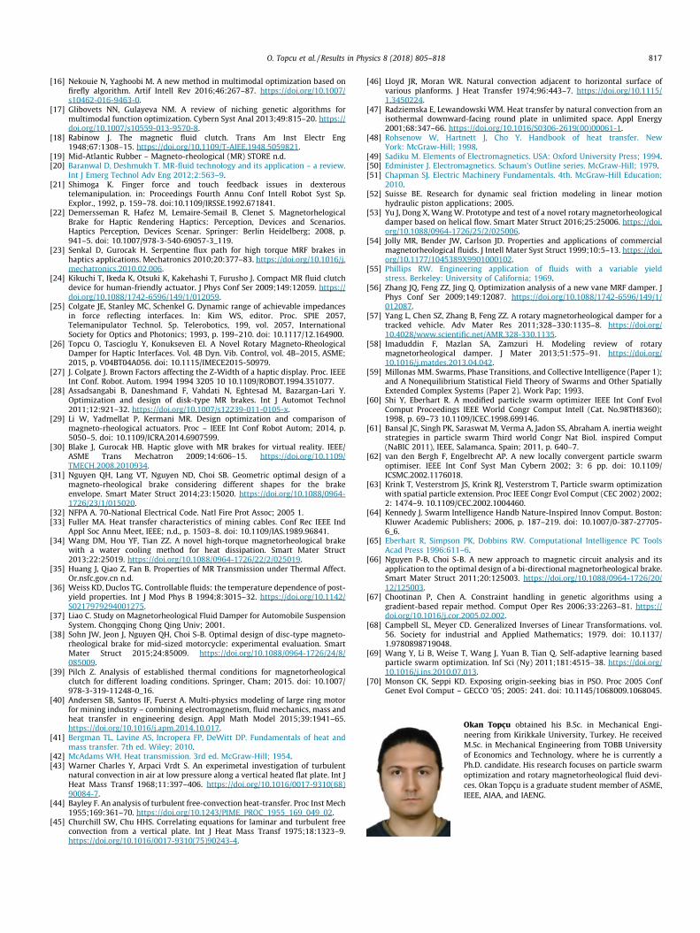
Figs. 15 and 16 show the magnetic field and heat transfer anal-ysis of the hybrid-type (device 0) MRF device at a current of 1.3A. Despite the fact that the hybrid-type favors a cylindrical geom-etry, it has disc geometry because of the mass factor in the costfunction.

Figs. 17 and 18 show the magnetic field and heat transferanalyzes of the disc type (device 1) MRF device at a currentof 1.0 A. Due to the coil winding and the maximum radiuslimitation, the geometry is thicker than conventional discgeometry.

Magnetic field analysis and heat transfer analysis of the rotaryflow-type MRF brake at a current of 1.8 A are given respectivelyin Fig. 19 in Fig. 20. The brake resembles the hybrid type and disctype devices. The flow channel of the flow type device is also deep-ened after optimization. Geometric constraints have forced thesethree devices to take a thick disc shape. The magnetic field analysisand the heat transfer analysis of the T-shape MRF brake at a cur-rent of 1.0 A are given respectively in Fig. 20 and Fig. 21. The brakehas cylindrical geometry unlike the other three designs. Likewisethis geometry, which is usually seen in drum-type devices, is dueto the outer radius limitation.

The regions used in the torque calculations are marked withdashed yellow lines in Fig. 16, Fig. 18, Fig. 20, and Fig. 22. The

MR fluid temperatures for device 0, device 1, device 2, anddevice 3 were obtained approximately 70 �C, 60 �C, 70 �C, and75 �C. It is seen that the temperature distribution changesdepending on the external surface area, position of coil winding,and power input.

Results of common PSO

The cost function dependent torque, mass, and power valuesobtained from the common PSO are given in Fig. 23.

In Table 4, the parameters of the designs obtained at the lowestcost are given.

Table 5 gives the characteristics of the devices which areachieved by common PSO. It is seen that the hunting PSO, whichhas the lowest cost function value of 0.091, is more successfulwhen Tables 3 and 5 are compared.

1st subswarm’s timing is 28.2 h, 2nd subswarm’s timing is22.5 h, and 3rd subswarm’s timing is 22.4 h. Total running timefor the hunting PSO and the common PSO is respectively 73.1and 195.8 h. Device 3 has two additional dimensional parameters,which have increased the simulation time by 54% compared toother devices. The hunting PSO required about 1/3 computationaltime compared to the common PSO. Furthermore hunting PSO

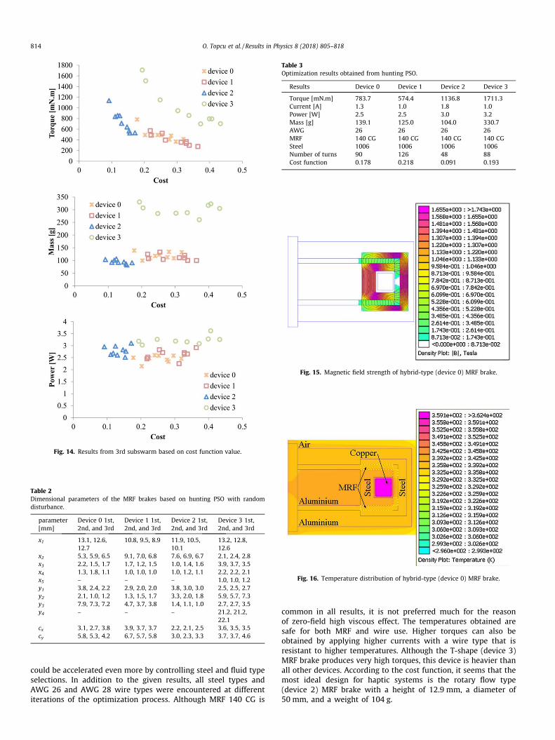
Fig. 14. Results from 3rd subswarm based on cost function value.

Table 2Dimensional parameters of the MRF brakes based on hunting PSO with randomdisturbance.

parameter[mm]

Device 0 1st,2nd, and 3rd

Device 1 1st,2nd, and 3rd

Device 2 1st,2nd, and 3rd

Device 3 1st,2nd, and 3rd

x1 13.1, 12.6,12.7

10.8, 9.5, 8.9 11.9, 10.5,10.1

13.2, 12.8,12.6

x2 5.3, 5.9, 6.5 9.1, 7.0, 6.8 7.6, 6.9, 6.7 2.1, 2.4, 2.8x3 2.2, 1.5, 1.7 1.7, 1.2, 1.5 1.0, 1.4, 1.6 3.9, 3.7, 3.5x4 1.3, 1.8, 1.1 1.0, 1.0, 1.0 1.0, 1.2, 1.1 2.2, 2.2, 2.1x5 – – – 1.0, 1.0, 1.2y1 3.8, 2.4, 2.2 2.9, 2.0, 2.0 3.8, 3.0, 3.0 2.5, 2.5, 2.7y2 2.1, 1.0, 1.2 1.3, 1.5, 1.7 3.3, 2.0, 1.8 5.9, 5.7, 7.3y3 7.9, 7.3, 7.2 4.7, 3.7, 3.8 1.4, 1.1, 1.0 2.7, 2.7, 3.5y4 – – – 21.2, 21.2,

22.1cx 3.1, 2.7, 3.8 3.9, 3.7, 3.7 2.2, 2.1, 2.5 3.6, 3.5, 3.5cy 5.8, 5.3, 4.2 6.7, 5.7, 5.8 3.0, 2.3, 3.3 3.7, 3.7, 4.6

Table 3Optimization results obtained from hunting PSO.

Results Device 0 Device 1 Device 2 Device 3

Torque [mN.m] 783.7 574.4 1136.8 1711.3Current [A] 1.3 1.0 1.8 1.0Power [W] 2.5 2.5 3.0 3.2Mass [g] 139.1 125.0 104.0 330.7AWG 26 26 26 26MRF 140 CG 140 CG 140 CG 140 CGSteel 1006 1006 1006 1006Number of turns 90 126 48 88Cost function 0.178 0.218 0.091 0.193

Fig. 15. Magnetic field strength of hybrid-type (device 0) MRF brake.

Fig. 16. Temperature distribution of hybrid-type (device 0) MRF brake.

814 O. Topcu et al. / Results in Physics 8 (2018) 805–818

could be accelerated even more by controlling steel and fluid typeselections. In addition to the given results, all steel types andAWG 26 and AWG 28 wire types were encountered at differentiterations of the optimization process. Although MRF 140 CG is

common in all results, it is not preferred much for the reasonof zero-field high viscous effect. The temperatures obtained aresafe for both MRF and wire use. Higher torques can also beobtained by applying higher currents with a wire type that isresistant to higher temperatures. Although the T-shape (device 3)MRF brake produces very high torques, this device is heavier thanall other devices. According to the cost function, it seems that themost ideal design for haptic systems is the rotary flow type(device 2) MRF brake with a height of 12.9 mm, a diameter of50 mm, and a weight of 104 g.

Fig. 17. Magnetic field strength of disc type (device 1) MRF brake.

Fig. 18. Temperature distribution of disc type (device 1) MRF brake.

Fig. 19. Magnetic field strength of rotary flow type (device 2) MRF brake.

Fig. 20. Temperature distribution of rotary flow type (device 2) MRF brake.

Fig. 21. Magnetic field strength of T-shape type (device 3) MRF brake.

Fig. 22. Temperature distribution of T-shape (device 3) MRF brake.

O. Topcu et al. / Results in Physics 8 (2018) 805–818 815

Conclusions and future work

In this paper four rotary MRF brake designs are optimized by asimple cost function which seeks the highest torque, lowest powerconsumption, and lightweight designs. The optimization processwas carried out by a modified PSO algorithm which was inspiredby a hunting party with task distribution. This successfully devel-oped and modified PSO algorithm with multiple subpopulationshas solved a multi-physics optimization problem. The modifiedPSO algorithm begins with a relatively large subpopulation withlimited resources. The first large subswarm is expected to uncovera solution space around the best possible solution. Narrowing ofthis search space is carried by a small subswarm with relatively

Fig. 23. Results obtained from common PSO.

Table 4Dimensional parameters of the MRF brakes based on common PSO with randomdisturbance.

parameter [mm] Device 0 Device 1 Device 2 Device 3

x1 11.6 4.3 9.2 12.4x2 5.2 12.3 7.4 1.9x3 1.5 2.0 1.2 3.7x4 3.8 1.2 1.2 1.2x5 – – – 1.0y1 3.0 4.3 3.1 1.5y2 1.4 2.1 2.6 4.8y3 7.1 5.6 1.0 2.6y4 – – – 16.2cx 3.1 2.1 3.2 3.1cy 5.1 7.2 4.5 3.3

Table 5Optimization results obtained from common PSO.

Results Device 0 Device 1 Device 2 Device 3

Torque [mN.m] 469.0 700.6 1136.8 1711.3Current [A] 1.3 1.3 1.3 1.3Power [W] 2.0 2.6 2.2 2.9Mass [g] 136.1 193.2 138.1 201.7AWG 26 26 26 26MRF 140 CG 140 CG 140 CG 140 CGSteel 1010 1006 1018 1010Number of turns 84 85 77 56Cost function 0.29 0.276 0.156 0.235

816 O. Topcu et al. / Results in Physics 8 (2018) 805–818

large resources that is fully capable of searching the space. Thelocating of optimal positions is carried out by the last subswarmwhich has also limited resources but has the knowledge of thesmall search space where the best solution resides. Obtainedresults sufficiently reveal the applicability of the modified PSOalgorithm in similar multi-physics problems. In future works, themodified PSO algorithm may be applied to solve the multimodalmulti-objective engineering optimization problems.

Declaration of conflicting interests

The author(s) declared no potential conflicts of interest withrespect to the research, authorship, and/or publication of thisarticle.

Funding

This research received no specific grant from any fundingagency in the public, commercial, or not-for-profit sectors.

Appendix A. Supplementary data

Supplementary data associated with this article can be found, inthe online version, at https://doi.org/10.1016/j.rinp.2018.01.007.

References

[1] Lari A, Khosravi A, Rajabi F. Controller design based on analysis and PSOalgorithm. ISA Trans 2014;53:517–23. https://doi.org/10.1016/j.isatra.2013.11.006.

[2] Chiou JS, Tsai SH, Liu MT. A PSO-based adaptive fuzzy PID-controllers. SimulModel Pract Theory 2012;26:49–59. https://doi.org/10.1016/j.simpat.2012.04.001.

[3] Letting LK, Munda JL, Hamam Y. Optimization of a fuzzy logic controller for PVgrid inverter control using S-function based PSO. Sol Energy2012;86:1689–700. https://doi.org/10.1016/j.solener.2012.03.018.

[4] Kennedy J, Eberhart C. Particle swarm optimization. In: Proceeding IEEE Int.Conf. Neural Networks, Perth, Australia; 1995, p. 1942–8.

[5] Reeves WT. Particle systems – a technique for modeling a class of fuzzyobjects. ACM SIGGRAPH Comput Graph 1983;17:359–75. https://doi.org/10.1145/964967.801167.

[6] Reynolds CW. Flocks, herds and schools: a distributed behavioral model. ACMSIGGRAPH Comput Graph 1987;21:25–34. https://doi.org/10.1145/37402.37406.

[7] Chang W. A modified particle swarm optimization with multiplesubpopulations for multimodal function optimization problems. Appl SoftComput J 2015;33:170–82. https://doi.org/10.1016/j.asoc.2015.04.002.

[8] Krishnanand KN, Ghose D. Glowworm swarm optimization for simultaneouscapture of multiple local optima of multimodal functions. Swarm Intell2009;3:87–124. https://doi.org/10.1007/s11721-008-0021-5.

[9] Yazdani S, Nezamabadi-Pour H, Kamyab S. A gravitational search algorithm formultimodal optimization. Swarm Evol Comput 2014;14:1–14. https://doi.org/10.1016/j.swevo.2013.08.001.

[10] Chen C-C. Two-layer particle swarm optimization for unconstrainedoptimization problems. Appl Soft Comput 2011;11:295–304. https://doi.org/10.1016/j.asoc.2009.11.020.

[11] Peng Y, Lu B-L. A hierarchical particle swarm optimizer with latin samplingbased memetic algorithm for numerical optimization. Appl Soft Comput 2012.https://doi.org/10.1016/j.asoc.2012.05.020.

[12] Wang H, Yang S, Ip WH, Wang D. A memetic particle swarm optimisationalgorithm for dynamic multi-modal optimisation problems. Int J Syst Sci2012;43:1268–83. https://doi.org/10.1080/00207721.2011.605966.

[13] Otani T, Suzuki R, Arita T. DE/isolated/1: a new mutation operator formultimodal optimization with differential evolution. Int J Mach Learn Cybern2013;4:99–105. https://doi.org/10.1007/s13042-012-0075-y.

[14] Kaveh A, Laknejadi K. A new multi-swarm multi-objective optimizationmethod for structural design. Adv Eng Softw 2013;58:54–69. https://doi.org/10.1016/j.advengsoft.2013.01.004.

[15] Goh CK, Tan KC, Liu DS, Chiam SC. A competitive and cooperative co-evolutionary approach to multi-objective particle swarm optimizationalgorithm design. Eur J Oper Res 2010;202:42–54. https://doi.org/10.1016/j.ejor.2009.05.005.

O. Topcu et al. / Results in Physics 8 (2018) 805–818 817

[16] Nekouie N, Yaghoobi M. A new method in multimodal optimization based onfirefly algorithm. Artif Intell Rev 2016;46:267–87. https://doi.org/10.1007/s10462-016-9463-0.

[17] Glibovets NN, Gulayeva NM. A review of niching genetic algorithms formultimodal function optimization. Cybern Syst Anal 2013;49:815–20. https://doi.org/10.1007/s10559-013-9570-8.

[18] Rabinow J. The magnetic fluid clutch. Trans Am Inst Electr Eng1948;67:1308–15. https://doi.org/10.1109/T-AIEE.1948.5059821.

[19] Mid-Atlantic Rubber – Magneto-rheological (MR) STORE n.d.[20] Baranwal D, Deshmukh T. MR-fluid technology and its application – a review.

Int J Emerg Technol Adv Eng 2012;2:563–9.[21] Shimoga K. Finger force and touch feedback issues in dexterous

telemanipulation. in: Proceedings Fourth Annu Conf Intell Robot Syst Sp.Explor., 1992, p. 159–78. doi:10.1109/IRSSE.1992.671841.

[22] Demersseman R, Hafez M, Lemaire-Semail B, Clenet S. MagnetorhelogicalBrake for Haptic Rendering Haptics: Perception, Devices and Scenarios.Haptics Perception, Devices Scenar. Springer: Berlin Heidelberg; 2008, p.941–5. doi: 10.1007/978-3-540-69057-3_119.

[23] Senkal D, Gurocak H. Serpentine flux path for high torque MRF brakes inhaptics applications. Mechatronics 2010;20:377–83. https://doi.org/10.1016/j.mechatronics.2010.02.006.

[24] Kikuchi T, Ikeda K, Otsuki K, Kakehashi T, Furusho J. Compact MR fluid clutchdevice for human-friendly actuator. J Phys Conf Ser 2009;149:12059. https://doi.org/10.1088/1742-6596/149/1/012059.

[25] Colgate JE, Stanley MC, Schenkel G. Dynamic range of achievable impedancesin force reflecting interfaces. In: Kim WS, editor. Proc. SPIE 2057,Telemanipulator Technol. Sp. Telerobotics, 199, vol. 2057, InternationalSociety for Optics and Photonics; 1993, p. 199–210. doi: 10.1117/12.164900.

[26] Topcu O, Tascioglu Y, Konukseven EI. A Novel Rotary Magneto-RheologicalDamper for Haptic Interfaces. Vol. 4B Dyn. Vib. Control, vol. 4B–2015, ASME;2015, p. V04BT04A056. doi: 10.1115/IMECE2015-50979.

[27] J. Colgate J. Brown Factors affecting the Z-Width of a haptic display. Proc. IEEEInt Conf. Robot. Autom. 1994 1994 3205 10 10.1109/ROBOT.1994.351077.

[28] Assadsangabi B, Daneshmand F, Vahdati N, Eghtesad M, Bazargan-Lari Y.Optimization and design of disk-type MR brakes. Int J Automot Technol2011;12:921–32. https://doi.org/10.1007/s12239-011-0105-x.

[29] Li W, Yadmellat P, Kermani MR. Design optimization and comparison ofmagneto-rheological actuators. Proc – IEEE Int Conf Robot Autom; 2014, p.5050–5. doi: 10.1109/ICRA.2014.6907599.

[30] Blake J, Gurocak HB. Haptic glove with MR brakes for virtual reality. IEEE/ASME Trans Mechatron 2009;14:606–15. https://doi.org/10.1109/TMECH.2008.2010934.

[31] Nguyen QH, Lang VT, Nguyen ND, Choi SB. Geometric optimal design of amagneto-rheological brake considering different shapes for the brakeenvelope. Smart Mater Struct 2014;23:15020. https://doi.org/10.1088/0964-1726/23/1/015020.

[32] NFPA A. 70-National Electrical Code. Natl Fire Prot Assoc; 2005 1.[33] Fuller MA. Heat transfer characteristics of mining cables. Conf Rec IEEE Ind

Appl Soc Annu Meet, IEEE; n.d., p. 1503–8. doi: 10.1109/IAS.1989.96841.[34] Wang DM, Hou YF, Tian ZZ. A novel high-torque magnetorheological brake

with a water cooling method for heat dissipation. Smart Mater Struct2013;22:25019. https://doi.org/10.1088/0964-1726/22/2/025019.

[35] Huang J, Qiao Z, Fan B. Properties of MR Transmission under Thermal Affect.Or.nsfc.gov.cn n.d.

[36] Weiss KD, Duclos TG. Controllable fluids: the temperature dependence of post-yield properties. Int J Mod Phys B 1994;8:3015–32. https://doi.org/10.1142/S0217979294001275.

[37] Liao C. Study on Magnetorheological Fluid Damper for Automobile SuspensionSystem. Chongqing Chong Qing Univ; 2001.

[38] Sohn JW, Jeon J, Nguyen QH, Choi S-B. Optimal design of disc-type magneto-rheological brake for mid-sized motorcycle: experimental evaluation. SmartMater Struct 2015;24:85009. https://doi.org/10.1088/0964-1726/24/8/085009.

[39] Pilch Z. Analysis of established thermal conditions for magnetorheologicalclutch for different loading conditions. Springer, Cham; 2015. doi: 10.1007/978-3-319-11248-0_16.

[40] Andersen SB, Santos IF, Fuerst A. Multi-physics modeling of large ring motorfor mining industry – combining electromagnetism, fluid mechanics, mass andheat transfer in engineering design. Appl Math Model 2015;39:1941–65.https://doi.org/10.1016/j.apm.2014.10.017.

[41] Bergman TL, Lavine AS, Incropera FP, DeWitt DP. Fundamentals of heat andmass transfer. 7th ed. Wiley; 2010.

[42] McAdams WH. Heat transmission. 3rd ed. McGraw-Hill; 1954.[43] Warner Charles Y, Arpaci Vrdt S. An experimetal investigation of turbulent

natural convection in air at low pressure along a vertical heated flat plate. Int JHeat Mass Transf 1968;11:397–406. https://doi.org/10.1016/0017-9310(68)90084-7.

[44] Bayley F. An analysis of turbulent free-convection heat-transfer. Proc Inst Mech1955;169:361–70. https://doi.org/10.1243/PIME_PROC_1955_169_049_02.

[45] Churchill SW, Chu HHS. Correlating equations for laminar and turbulent freeconvection from a vertical plate. Int J Heat Mass Transf 1975;18:1323–9.https://doi.org/10.1016/0017-9310(75)90243-4.

[46] Lloyd JR, Moran WR. Natural convection adjacent to horizontal surface ofvarious planforms. J Heat Transfer 1974;96:443–7. https://doi.org/10.1115/1.3450224.

[47] Radziemska E, Lewandowski WM. Heat transfer by natural convection from anisothermal downward-facing round plate in unlimited space. Appl Energy2001;68:347–66. https://doi.org/10.1016/S0306-2619(00)00061-1.

[48] Rohsenow W, Hartnett J, Cho Y. Handbook of heat transfer. NewYork: McGraw-Hill; 1998.

[49] Sadiku M. Elements of Electromagnetics. USA: Oxford University Press; 1994.[50] Edminister J. Electromagnetics. Schaum’s Outline series. McGraw-Hill; 1979.[51] Chapman SJ. Electric Machinery Fundamentals. 4th. McGraw-Hill Education;

2010.[52] Suisse BE. Research for dynamic seal friction modeling in linear motion

hydraulic piston applications; 2005.[53] Yu J, Dong X, WangW. Prototype and test of a novel rotary magnetorheological

damper based on helical flow. Smart Mater Struct 2016;25:25006. https://doi.org/10.1088/0964-1726/25/2/025006.

[54] Jolly MR, Bender JW, Carlson JD. Properties and applications of commercialmagnetorheological fluids. J Intell Mater Syst Struct 1999;10:5–13. https://doi.org/10.1177/1045389X9901000102.

[55] Phillips RW. Engineering application of fluids with a variable yieldstress. Berkeley: University of California; 1969.

[56] Zhang JQ, Feng ZZ, Jing Q. Optimization analysis of a new vane MRF damper. JPhys Conf Ser 2009;149:12087. https://doi.org/10.1088/1742-6596/149/1/012087.

[57] Yang L, Chen SZ, Zhang B, Feng ZZ. A rotary magnetorheological damper for atracked vehicle. Adv Mater Res 2011;328–330:1135–8. https://doi.org/10.4028/www.scientific.net/AMR.328-330.1135.

[58] Imaduddin F, Mazlan SA, Zamzuri H. Modeling review of rotarymagnetorheological damper. J Mater 2013;51:575–91. https://doi.org/10.1016/j.matdes.2013.04.042.

[59] Millonas MM. Swarms, Phase Transitions, and Collective Intelligence (Paper 1);and A Nonequilibrium Statistical Field Theory of Swarms and Other SpatiallyExtended Complex Systems (Paper 2). Work Pap; 1993.

[60] Shi Y, Eberhart R. A modified particle swarm optimizer IEEE Int Conf EvolComput Proceedings IEEE World Congr Comput Intell (Cat. No.98TH8360);1998, p. 69–73 10.1109/ICEC.1998.699146.

[61] Bansal JC, Singh PK, Saraswat M, Verma A, Jadon SS, Abraham A. inertia weightstrategies in particle swarm Third world Congr Nat Biol. inspired Comput(NaBIC 2011), IEEE, Salamanca, Spain; 2011, p. 640–7.

[62] van den Bergh F, Engelbrecht AP. A new locally convergent particle swarmoptimiser. IEEE Int Conf Syst Man Cybern 2002; 3: 6 pp. doi: 10.1109/ICSMC.2002.1176018.

[63] Krink T, Vesterstrom JS, Krink RJ, Vesterstrom T, Particle swarm optimizationwith spatial particle extension. Proc IEEE Congr Evol Comput (CEC 2002) 2002;2: 1474–9. 10.1109/CEC.2002.1004460.

[64] Kennedy J. Swarm Intelligence Handb Nature-Inspired Innov Comput. Boston:Kluwer Academic Publishers; 2006, p. 187–219. doi: 10.1007/0-387-27705-6_6.

[65] Eberhart R, Simpson PK, Dobbins RW. Computational Intelligence PC ToolsAcad Press 1996:611–6.

[66] Nguyen P-B, Choi S-B. A new approach to magnetic circuit analysis and itsapplication to the optimal design of a bi-directional magnetorheological brake.Smart Mater Struct 2011;20:125003. https://doi.org/10.1088/0964-1726/20/12/125003.

[67] Chootinan P, Chen A. Constraint handling in genetic algorithms using agradient-based repair method. Comput Oper Res 2006;33:2263–81. https://doi.org/10.1016/j.cor.2005.02.002.

[68] Campbell SL, Meyer CD. Generalized Inverses of Linear Transformations. vol.56. Society for industrial and Applied Mathematics; 1979. doi: 10.1137/1.9780898719048.

[69] Wang Y, Li B, Weise T, Wang J, Yuan B, Tian Q. Self-adaptive learning basedparticle swarm optimization. Inf Sci (Ny) 2011;181:4515–38. https://doi.org/10.1016/j.ins.2010.07.013.

[70] Monson CK, Seppi KD. Exposing origin-seeking bias in PSO. Proc 2005 ConfGenet Evol Comput – GECCO ’05; 2005: 241. doi: 10.1145/1068009.1068045.

Okan Topçu obtained his B.Sc. in Mechanical Engi-neering from Kirikkale University, Turkey. He receivedM.Sc. in Mechanical Engineering from TOBB Universityof Economics and Technology, where he is currently aPh.D. candidate. His research focuses on particle swarmoptimization and rotary magnetorheological fluid devi-ces. Okan Topçu is a graduate student member of ASME,IEEE, AIAA, and IAENG.

818 O. Topcu et al. / Results in Physics 8 (2018) 805–818

Yigit Tas�cıoglu received his B.S. in Mechanical Engi-neering from Middle East Technical University, M.Sc.and Ph.D. in Mechatronics from Loughborough Univer-sity. Since 2006, he is with the Mechanical EngineeringDepartment, TOBB University of Economics and Tech-nology. He is also the founding coordinator of theMechatronics Minor Program.

E. _Ilhan Konukseven obtained Ph.D. degree inMechanical Engineering from METU. During his Post-Doc studies he has focused on mobile robotics andsensor based motion planning at Mechanical Engineer-ing Department, Carnegie Mellon University. Hisresearch interests focus on robotics, robotic machining& deburring, virtual reality, haptic devices, sensor basedmotion planning and mobile robotics.