Retail Redlining: 

Are gasoline prices higher in poor and minority neighborhoods?  by 

Caitlin Knowles Myers Grace Close, Laurice Fox, John William Meyer, and Madeline Niemi 

 August, 2009 

 

MIDDLEBURY COLLEGE ECONOMICS DISCUSSION PAPER NO. 09-06

DEPARTMENT OF ECONOMICS MIDDLEBURY COLLEGE

MIDDLEBURY, VERMONT 05753

http://www.middlebury.edu/~econ

Retail Redlining:

Are gasoline prices higher in poor and minority

neighborhoods?

Caitlin Knowles MyersGrace Close, Laurice Fox, John William Meyer, and Madeline Niemi∗

August 18, 2009

Abstract

Higher retail prices are frequently cited as a cost of living in poor, mi-nority neighborhoods. However, the empirical evidence, which primarilycomes from the grocery gap literature on food prices, has been mixed.This study uses new data on retail gasoline prices in three major U.S.cities to provide evidence on the relationship between neighborhood char-acteristics and consumer prices. We find that gasoline prices do not varygreatly with neighborhood racial composition, but that prices are higherin poor neighborhoods. For a 10 percentage point increase in the percentof families with incomes below the poverty line relative to families withincomes between 1 and 2 times the poverty line, retail gasoline prices areestimated to increase by an average of 0.70 percent. This differential isreduced to 0.22 percent once we add controls for costs, competition, anddemand. Finally, we provide evidence that the remaining, small, pricedifferential for poor neighborhoods is likely the result of traditional pricediscrimination in response to less competition and/or more inelastic de-mand in these locations.

JEL Classification: J15, J16Keywords: consumer prices, consumer market discrimination, race dis-crimination, price discrimination, redlining

∗Caitlin Knowles Myers is Assistant Professor, Department of Economics, MiddleburyCollege, Middlebury, VT 05753 and research fellow, IZA. The remaining authors were studentsin an undergraduate seminar who were instrumental in the planning, implementation, andanalysis associated with this project. We wish to thank Jack Cuneo for his assistance inusing ArcGIS to geocode gas stations and provide several geographic variables, and CarrieMacFarlane and Brenda Ellis for their assistance with ArcGIS and Geolytics software. We alsowish to thank the remaining students from an undergraduate seminar who assisted with thestation surveys: Harrison Brown, Michael Campbell, Matthew Engel, Ryan Fink, AnnabelleFowler, Daniel Haluska, Christopher Hench, Winslow Hicks, Blake Johnson, JiaHao Li, QuincyLiao, Shenique Moxey, Cameron Poole, Mona Quarless, Leah Shackleton, and Mary Walsh.

Anyone who has ever struggled with poverty knows how extremely expensive itis to be poor...Go shopping one day in Harlem– for anything– and compare

Harlem prices and quality with those downtown.James Baldwin, Nobody Knows My Name, 1961

It’s not that these businesses are saying ‘You, black people, you get out of my[establishment].’ They are saying ‘Come on in, but we’re going to rip you off.’Allison Bethel, Florida Assistant Attorney General, in U.S. News and World Report, 2000

1 Introduction

The economics literature on discrimination in consumer markets is dominated

by studies of differences in negotiated prices in two markets: housing (e.g.,

Yinger, 1986, 1995; Ondrich et al., 2003; Myers, 2004) and automobiles (e.g.,

Ayres and Siegelman, 1995; Goldberg, 1996). A few additional studies examine

price differentials in smaller markets in which prices are also negotiated such

as trading cards (List, 2004) and car repairs (Gneezy and List, 2004). Less

evidence is available from the numerous consumer markets in which prices are

publicly posted and fixed. In this situation, individually targeted racial price

discrimination is unlikely because, as Siegelman (1998) points out, it would re-

quire the flagrant and illegal display of different prices for whites and minorities.

However, firms may still adopt practices that increase the probability that mi-

norities or other targeted groups will pay higher prices. We use data on gasoline

prices and station characteristics from three metropolitan areas to test for one

such practice, commonly referred to as “retail redlining.”

Following D’Rozario and Williams (2005), we define “retail redlining” as a

practice among retailers that results in lower quality goods and services and/or

higher prices in areas with large minority or poor populations. Claims of retail

redlining arise regularly in both academic sources and the popular press, often

involving catch phrases such as “the poor pay more,” ”the high price of poverty,”

or “the poorer you are the more things cost” (e.g., Sturdivant, 1969; Downing,

1

2007; Brown, 2009). Accusations of retail redlining also arise in courtrooms,

and politics. GM, Wal-Mart, Burger King, Domino’s Pizza, and KB Toys have

been sued for discriminatory practices in minority neighborhoods (Jelisavcic,

1996; Smith, 1996; Fuller, 1998; Kaplan, 2000); in 1992 the mayor of Los Angeles

touted the need for more equal access to supermarkets following the Los Angeles

riots; and, in 2009, Illinois Senator Roland Burris introduced a request to the

annual federal appropriations bill for a campaign to fight retail redlining on

Chicago’s south side (Shaffer, 2002; Burris, 2009).

The bulk of the empirical evidence on retail redlining comes from the large

“grocery gap” literature, which explores variations across neighborhoods in the

accessibility, quality, and price of food sold at grocery stores. Much of this

evidence suggests that grocery prices are higher in inner-city neighborhoods

and that this is largely explained by the lack of large chain stores in these areas

(Hall, 1983; Kaufman et al., 1997; Chung and Myers, 1999; Shaffer, 2002). By

contrast, (Hayes, 2000), using a large nationally representative sample of price

data from the sampling frame used to construct the Consumer Price Index,

finds that prices are lower in poor neighborhoods but that the discount is not

constant across races. Poor whites and Hispanics receive discounts, but poor

blacks pay similar prices as affluent whites. Turning to the market for prepared

food, Graddy (1997) finds that fast food meal prices increase by about 5 percent

for a 50 percentage point increase in the percent black in a zip code.

While food, which makes up a large portion of consumer budgets, is an

important candidate for study of inter-neighborhood price variations, accusa-

tions of retail redlining extend beyond this single market. We provide evidence

from a hitherto unexamined market: retail gasoline. There are several reasons

to consider retail gasoline beyond the benefits of deviating from the extensive

literature on food prices. First, like groceries, gasoline makes up a relatively

large portion of the average consumer budget: 4.8 percent as compared to 7.0

2

percent for food purchased for home consumption (U.S. Department of Labor,

Bureau of Labor Statistics, 2008). Moreover, gasoline represents an important

commodity for the poor as well as for the more well-to-do. Private vehicles are

the dominant mode of travel even among households with annual income be-

low $20,000; three-quarters of these households own at least one vehicle, three

quarters of their travel is done in private vehicles, and gasoline makes up 5.1

percent of their consumption expenditures (Pucher and Renne, 2003; U.S. De-

partment of Labor, Bureau of Labor Statistics, 2008). A second reason for

considering the market for gasoline is that the grocery gap literature is compli-

cated by the heterogeneity of stores, products, and quality. Gasoline stations

are considerably more homogenous in terms of size and, after controlling for

branding, quality. This allows us to more precisely identify price differentials

for an identical good. Finally, anecdotal evidence and accusations in the popu-

lar press suggest that gasoline prices vary between stations and neighborhoods

(e.g., Douglas and Cohn, 2005; Rose, 2007), and any such variations have the

potential to be correlated with race and income characteristics.

We combine three sources of survey data to produce a panel of daily price

observations over the course of a year for nearly all of the gas stations in the

Atlanta, Detroit, and Philadelphia metropolitan areas. We examine the re-

lationship between prices and neighborhood racial and income characteristics

with additional controls for costs and demand. The results indicate that prices

do not vary greatly with neighborhood racial composition, but that prices are

slightly higher in poorer neighborhoods.

2 A model of retail redlining

As defined, retail redlining describes only the presence of inter-neighborhood

price differentials, not their source. Such price differentials may represent

3

animus-based discrimination or price discrimination in response to variation

in the elasticity of demand. However, inter-neighborhood price differentials also

may arise in perfectly competitive markets due to differences in costs between

neighborhoods. In fact, firms accused of retail redlining on the basis of race

often respond by claiming that, to the extent that price differentials exist, they

are the result of cost-related factors such as crime (D’Rozario and Williams,

2005).

To account for these possibilities, we adopt the flexible model used by

Graddy (1997) and based on the “new empirical industrial organization” as

described by Bresnahan (1989). Price setting conduct of firm i in market area

j at time t follows the general relation

Pjt +∂P (Qjt)

∂QjtQijtθijt = MCijt (1)

where Pjt is the price in market area j at time t, ∂P (Qjt)/∂Qjt is the derivative

of the inverse demand function, Qijt is quantity sold by firm i, and MC is

marginal cost for firm i. θijt indexes firm competitiveness, with increasing values

reflecting increasing distance from perfect competition. For instance, if θijt = 0,

a firm follows the perfectly competitive strategy of equating price to marginal

cost. If θijt = 1, a firm follows the monopoly strategy of equating monopoly

marginal revenue to marginal cost (for a full discussion, see Bresnahan, 1989).

Assuming constant elasticity of demand, ε, Qijt can be substituted out and

Equation 1 can be expressed as Pjt = MCijt/[1 + (1/ε)θijt]. Taking logs,

log(Pjt) = log(MCijt) − log(1 + (1/ε)θijt). (2)

Our last step is to introduce the possibility of animus-based discrimination

by incorporating a discrimination coefficient a la Becker (1957). Let bj ∈ [0, 1]

be the proportion of residents of neighborhood j who are black and let d ∈ [0, 1]

4

represent the discrimination coefficient for firms. Firms act as if the price they

receive in neighborhood j at time t is Pjt(1 − dbj) so that in the presence of

discriminatory firms (d > 0), firms act as if marginal revenue is decreasing in

the black population of a neighborhood. Equation 2 now can be written as

log(Pjt) = log(MCijt) − log(1 + (1/ε)θijt) − log(1 − dbj). (3)

If we assume that neighborhoods represent individual market areas, prices

could be higher in neighborhood j for four reasons: (1) higher marginal costs,

(2) less competition, (3) less elastic demand in the presence of imperfect com-

petition, which allows for classic price discrimination, or (4) a greater presence

of some attribute (e.g., race) on which all firms engage in animus-based discrim-

ination. Our empirical strategy is to first determine whether there is evidence

of price variation between neighborhoods with different racial and income com-

positions. To the extent that any such differentials remain after controlling

for costs and competitiveness, we discuss and explore whether they represent

animus-based discrimination.

3 Data

We combine three sources of data: gasoline price data from Oil Price Infor-

mational Service (OPIS), neighborhood characteristics from the 2000 Decennial

Census, and individual station characteristics obtained via telephone survey.

Gasoline price data were purchased from OPIS, which monitors retail gaso-

line prices across the United States and Canada by observing “fleet card” trans-

actions: special credit card transactions for groups of vehicles owned or leased

by businesses or government agencies. The data include daily price observa-

tions for regular unleaded gasoline purchased between December 1, 2007 and

November 30, 2008 at stations in three metropolitan areas: Atlanta, Detroit,

5

and Philadelphia. A station enters the OPIS sample on any day in which a fleet

card is used to purchase gasoline there. Because fleet card transactions are quite

common, OPIS estimates that nearly all of the gasoline stations and convenience

stores in a metropolitan area will incur at least one fleet card transaction in a

year and, hence, be represented in the sample. The exceptions will primarily be

stations that do not accept credit cards.

The raw gasoline price data form an unbalanced panel of 1.4 million station-

price observations for 5,736 unique stations. Of these, 322 stations are observed

on fewer than 20 days and have been dropped from the sample. Some of these

stations appear to have entered or exited the market during the sample period,

while others appear to be automobile dealerships where fleet cards are occasion-

ally used to purchase gasoline. The data also include the name and brand of

the station and the station address.

Information about the area surrounding each gasoline station was collected

using ArcGIS software and census data. ArcGIS was used to identify the ge-

ographic coordinates of each station based on the street address provided by

OPIS. Of the 5,414 stations observed twenty or more times by OPIS, the coor-

dinates of 96.5 percent of the stations could be identified in this manner; the

remaining 191 stations also have been dropped from the sample. ArcGIS was

then used to note the number of nearby competing stations and the distance

to major roads. Finally, the census tract containing each station was identified

based on the station’s geographic coordinates, and variables measuring census

tract characteristics were collected from the 2000 U.S. Census. An additional 20

stations have been dropped from the sample because complete characteristics

of the surrounding census tract were not available.

Data measuring individual station characteristics such as capacity and the

presence of a car wash were collected by telephone survey of a subsample of sta-

tions. Undergraduate students contacted a random subsample of 1,745 stations

6

by phone and asked a brief series of survey questions which are reproduced in

Appendix A. Of the contacted stations, 1,131 either had an invalid phone num-

ber, declined to begin the survey, or began but did not complete the survey. Six

hundred and fourteen, or 35 percent, of the surveys were completed. However,

42 of these stations were later dropped from the sample because we could not

identify their geographic coordinates using ArcGIS or because they were ob-

served fewer than 20 times during the sampled year. An additional 5 stations

were dropped because the telephone surveyor mis-coded a variable.1

Table 1 presents descriptive statistics for stations in the final sample. After

removing stations with limited price observations or incomplete geographic vari-

ables, there are 5,203 station observations (2,288 in Atlanta, 1,612 in Detroit,

and 1,302 in Philadelphia). The average station is observed on 250 of the 366

possible days in the sample period (which covers a leap year). The available

variables measure or proxy for the price of gasoline, neighborhood racial and

income characteristics, costs, the level of competitiveness, and demand. We

describe the variables in more detail below.

Price

OPIS records the price posted at the pump, which is inclusive of applicable

gasoline taxes and exclusive of any discounts or rebates that may be offered to

fleet card holders. In the period and metropolitan areas covered by the sample,

applicable gasoline taxes include a federal excise tax and state taxes that can

include excise taxes, state sales tax, and environmental surcharges. Local taxes

are applied in only one of the four states in the sample, Georgia, were they

range from 6 to 7 percent and are pre-paid based on the state’s announced

average sales price of gasoline. We calculate the price net of all taxes using1Response to the telephone surveys is clearly non-random. However, as shown in Table 1,

the observable characteristics of surveyed stations are quite similar to those of non-surveyedstations.

7

information from the American Petroleum Institute and Georgia Department

of Revenue (The American Petroleum Institute, 2009; Georgia Department of

Revenue, 2007a,b, 2008, 2009). Because the incidence of state and local taxes

falls almost entirely on consumers (Chouinard and Perloff, 2004), we choose to

use the net price as the outcome variable in our analysis with the assumption

that it more accurately reflects the pricing behavior of retailers. However, not

surprisingly given the limited local variation in taxes in the sample, the results

are quite similar using gross price and state indicator variables. As reported

in Table 1, the average price of gasoline over the course of the year in which

stations were observed was $3.34 inclusive of taxes and $2.86 exclusive of taxes.

Racial and income characteristics

The racial composition of the census tract surrounding a station was obtained

from the 2000 U.S. Census. Respondents classify themselves into one or more of

multiple racial and ethnic categories, which we use to create four mutually ex-

clusive and collectively exhaustive categories: white, black, Hispanic, and other.

The percent white in a tract measures the percent of respondents reporting that

they are non-Hispanic and white alone; similarly, the percent black in a tract

measures the percent of respondents who are non-Hispanic and black alone. The

percent “other” is the percent of non-Hispanic respondents reporting that they

are Asian, American Indian, some other single race, or more than one race.2 The

percent Hispanic is the percent of residents belonging to any racial category who

reported that they are Hispanic. Table 1 includes summary statistics for these

variables; the average station in the sample is located in a neighborhood that is

69 percent white, 21 percent black, 5 percent Hispanic, and 5 percent other.

Turning to income, we use a set of three income variables from the census

that measure the percent of families in a census tract with incomes placing2Fewer than 2 percent of respondents in the sample indicated that they belonged to multiple

racial categories.

8

them below the poverty line (poor), between the poverty line and two times

the poverty line (lower-middle income), and above two times the poverty line

(middle-upper income). Using these three categories allows for a non-linear

relationship similar to that reported by Frankel and Gould (2001), who found

that retails prices are increasing with both the percent of families who are poor

and who are middle-upper income. As reported in the summary statistics in

Table 1, the average station is located in a neighborood in which 10 percent

of families are poor, 14 percent are lower-middle income, and 76 percent are

middle-upper income.3

Costs

Three quarters of the retail price of gasoline is accounted for by the wholesale

price of refined gasoline (Energy Information Administration, 2009). Time fixed

effects account for temporal fluctuations in the price of crude oil, while state

fixed effects account for differences in the wholesale price of gasoline arising

due to regional variation in the costs of crude oil, refining, and transportation.

However, the wholesale price of gasoline paid by individual stations also varies

within a metropolitan area at any given time due to variation in branding and

the ownership structure, which we describe.

Branded gasoline stations, which make up about 83 percent of the market,

display the name of a major refiner or wholesale marketer such as Shell or

Texaco and sell the wholesaler’s brand of gasoline, which includes proprietary

additives (Kleit, 2003). Branded gasoline stations can roughly be divided into

one of three ownership structures: owned and operated by the wholesaler (19

percent of branded stations nationwide), owned by the wholesaler and leased by

an independent dealer (20 percent of branded stations), and owned and operated

3Because so many respondents fall in the middle-upper income bracket, it would be prefer-able to divide it into smaller categories. However, the Census Bureau does not provide a moredetailed breakdown of family income distributions above two times the poverty line.

9

by an independent dealer (61 percent of branded stations) (Meyer and Fischer,

2004). Stations in the first two categories typically receive gasoline directly from

the wholesaler, while stations in the last category typically receive gasoline from

“jobbers,” independent contractors who gain the right to franchise a brand in

a certain area. Unbranded stations, which make up the remaining 17 percent

of the gasoline market, typically purchase gasoline from a refiner that does not

have a branded presence in the retail gasoline market (Kleit, 2003).

Branded stations that are supplied directly by the wholesaler may be sub-

ject to “zone pricing,” a practice in which branded wholesalers define a price

zone as a contiguous set of stations within a small geographic area that face a

similar market environment. A wholesaler charges all direct-supplied retailers

in the price zone a common wholesale price (Meyer and Fischer, 2004). Zone-

pricing clearly suggests the existence of inter-neighborhood price differentials.

However, retailers who buy from unbranded wholesalers or jobbers at a uniform

regional wholesale price still presumably price retail gasoline according to local

market conditions. To the extent that zone pricing reflects market conditions

but does not itself increase market power, one would expect inter-neighborhood

variation in prices regardless of whether zone pricing is employed in a certain

neighborhood.4.

To account for differences in wholesale prices due to branded status, we

include a single branded variable that indicates a station sells branded gasoline.5

Accounting for price differences due to ownership structure is more difficult,

and we only attempt to do so with stations that were surveyed by telephone.4For more detailed theoretical and empirical evidence on ownership structure and retail

prices, see Shepard (1991); Taylor (2000); Kleit (2003); Meyer and Fischer (2004)5The branded variable indicates that a station displays one of the following brands: BP,

Chevron, Citgo, Conoco, Exxon, Getty, Gulf, Hess, Lukoil, Marathon Ashland, Mobil, Phillips66, Shell, Sunoco, Texaco, and Valero. The results are robust to substituting a series ofindicators for each of the 19 specific retail station types that are observed most at least thirtytimes in the data: 7-eleven, BP, Chevron, Citgo, Clark, Exxon, Getty, Gulf, Hess, Kroger,Lukoil, Marathon, Mobil, Quik Trip, Racetrac, Sams, Shell, Speedway, Sunoco, Texas, Valero,and Wawa.

10

It is not feasible to collect information on ownership structure and wholesale

supply via telephone because many station employees are not aware of this type

of information. Instead, we asked the employee answering the phone whether

the station owner regularly works behind the counter and assume that stations

where this is the case are more likely to be operated by an independent dealer.

We also collected information on three variables that Taylor (2000) found to be

correlated with ownership structure because of their relationship to monitoring

effort. These are indicators for whether the station has repair bays (as proxied

by offering oil changes), full service pumps, and a convenience store (as proxied

by selling milk by the gallon).6 Stations offering repair service or full service

are more likely to be owned or leased by an independent dealer, while stations

with a convenience store are more likely to be owned and operated by a branded

wholesaler (Taylor, 2000).

In addition to variables controlling for brand and proxying for ownership

structure, we include several other controls for costs. Real estate costs are

represented by the log of the median value of owner-occupied housing in the

surrounding census tract. Population density, which is correlated with house

values, also is included. For stations that were surveyed by telephone, we have

a series of additional variables measuring station characteristics including indi-

cators for the presence of a car wash and restaurant. A measure of the number

of gasoline pumps, capacity, represents possible economies of scale associated

with larger stations.

A final concern is that the local crime rate is correlated with gasoline price

either because of the direct cost of crimes committed or because of indirect

costs due to higher insurance rates or the need to pay compensating differen-

tials to employees who feel that working at a station in a high crime area is6All stations in New Jersey are full service. Stations in other states are coded as full service

if they routinely pump gas for customers at any of their pumps.

11

risky. Because of the paucity of crime data available at a small geographic level,

researchers typically control for crime at a broad geographic level such as mu-

nicipality or zip code (e.g., Graddy, 1997; Hayes, 2000). We attempt to create

a proxy variable measuring crime at a smaller local level by asking telephone

survey respondents to rank the severity of crime in the neighborhood on a scale

of one to ten and coding stations with ratings in the top third (greater than a

three) as having severe local crime. Although this measure has the advantage of

presumably being more local to a gas station than crime data for the entire mu-

nicipality as supplied by FBI Uniform Crime Reports, it has the disadvantage

of being subjective. We discuss an alternative measure in Section 6.

Competitiveness and Demand

Our model predicts that prices will be higher in neighborhoods where sta-

tions have greater market power because of some combination of fewer com-

petitors and/or more inelastic demand. We measure the number of competing

stations within a 1 kilometer radius of each station in the sample using ArcGIS

software. We proxy for the elasticity of demand using a set of variables that

we expect to relate to search costs. The first two, km to nearest interstate

and km to nearest highway, measure the distance from each station to the

nearest limited access highway and major non-limited access highway, respec-

tively. We assume that search costs are lower, and demand is more elastic, for

vehicles traveling on major roads because they will typically encounter more

gasoline stations on a trip. The remaining variables that proxy for demand are

pct commute by car, avg commute time, pct of households with 1 vehicle,

and pct of households with 2+ vehicles. We expect that demand is higher

in areas with more vehicles both because those vehicles require gasoline and

because car ownership is positively correlated with unobserved heterogeneity in

income. However, we also expect that demand is more elastic in areas with

12

more vehicles, more commuters, and longer average commutes because search

costs are lower for households that drive more.

4 Empirical Model

The analysis is based on a two-way mixed error component specification:

log(Pijt) = α + Njβ + Cijδ + Dijγ + υi + υt + εijt. (4)

Pijt is the price of regular octane gasoline observed at station i in neighborhood

j on week t. Nj is a vector of racial and income characteristics of neighborhood

j, Cij is a vector of proxies for costs for station i in neighborhood j, and Dij

is a vector of proxies for the competitiveness of station i in neighborhood j.

The error term includes a station-specific component, υi, and a time-specific

component, υt. The final term, εijt, represents a classical random disturbance.

The time-specific component of the error term is treated as a fixed effect so

that identification is based on the deviation of station i’s prices from the mean

price observed during week t. Because all of the explanatory variables are time-

invariant, the station component of the error term is by necessity treated as

random.7 The (un-testable) assumption that we must make is that the unob-

served station effects are not correlated with the regressors. Even if this is not

the case, we still are able to address our first question– Are gasoline prices higher

in poor and minority neighborhoods?– although we would be unsure whether

any observed relationship is the direct effect of race and income or the result

of some unobserved factor that is correlated with neighborhood and/or station

characteristics.7For more on two-way error component specifications, see Baltagi (2008). One might

also wish to consider a three-way error component model with station random effects thatare nested within neighborhood random effects. However, it is very difficult to perform thecomputations required to estimate such a specification because of the large size of the dataset (5,203 stations in 2,117 neighborhoods observed over 52 weeks).

13

5 Do gasoline prices vary with neighborhood char-acteristics?

Table 2 reports the estimated coefficients for the two-way error component spec-

ification with week fixed effects and station random effects.8 The estimates in

Model 1 indicate the mean price differentials observed across neighborhoods with

different racial and income compositions without additional control variables.

In Model 2 we add the variables measuring cost, competition, and demand char-

acteristics that we are able to observe for all stations in the sample. In Model

3 we add additional control variables for station characteristics obtained via

telephone survey, which reduces the sample size accordingly.9

The estimated coefficients for the variables measuring neighborhood racial

composition are small in magnitude and, with one exception, statistically in-

significant. This suggests that there are not large price differentials associated

with race. The coefficient on percent black in Model 1, for example, indicates

that for a 10 percentage point increase in the percent black in a neighborhood,

retail gasoline prices are about 0.02 percent higher (p-value= 0.15). Once we

control for costs, competition, and demand in Models 2 and 3 this differential is

of even smaller magnitude, negative, and highly statistically insignificant. This

suggests that to the extent that (small and statistically insignificant) positive

price effects of minority composition were observed in Model 1, they can be

accounted for by differences in costs, competition, and demand. Moreover, the

single result that is statistically significant indicates that rather than paying a

premium, prices are actually decreasing with the presence of other residents.8Specification tests support the validity of this specification. Breusch Pagan tests indicate

that station random effects are appropriate (p-value< 0.01 for Models 1-3). Hausman testsalso indicate that week fixed effects are appropriate (p-value< 0.01 for Models 1-3). However,while the differences in coefficients between models with and without week fixed effects arestatistically significant, they are not large in magnitude.

9The results in Model 3 may differ from Model 2 because of the change in the sample aswell as because of the additional control variables. However, if we estimate Model 2 usingonly the stations that appear in the sample in Model 3, we get similar point estimates.

14

By contrast to the race results, the coefficients on the income measures

are of larger magnitude as well as highly statistically significant. Like Frankel

and Gould (2001), we find that prices are lowest in neighborhoods with more

lower-middle income families and higher in neighborhoods both with more poor

residents and with more middle-upper income residents. The estimates in Model

1 indicate that for a 10 percentage point increase in the percent of middle-

upper relative to lower-middle income families, retail gasoline prices are 0.48

percent higher (p-value< 0.01). And, for a 10 percentage point increase in

the percent of poor relative to lower-middle income families in a neighborhood,

retail gasoline prices are 0.70 percent higher (p-value< 0.01). At the sample

average gasoline price of $2.86 (net of taxes), a 0.70 percent increase represents

a premium of about $0.02 per gallon of gas. As an alternative way to think

about the magnitude of this effect, consider the spatial variation in gasoline

prices across a city. We observe that the average standard deviation in gasoline

prices observed in a given city on a given day in our sample is about 2.8 percent

of the mean. Hence, a 0.70 percent premium paid for a 10 percentage point

increase in the percent of families in a neighborhood that are poor represents

about a quarter of a standard deviation increase in gasoline prices.

The relationship between income and prices diminishes in Models 2 and 3,

suggesting that the premiums paid in poor and middle-upper income neighbor-

hoods can be partially explained by costs and competition characteristics that

are correlated with income. The estimated coefficient on pct > 2 times poverty

line becomes much smaller as well as statistically insignificant in Models 2 and

3. The coefficient on the percent of families below the poverty line remains

statistically significant in Model 2, although its magnitude is reduced by two-

thirds; for a 10 percentage point increase in the percent of poor families relative

to lower-middle income families, gasoline prices are estimated to be 0.22 per-

cent higher. The corresponding point estimate is 0.37 percent higher in Model

15

3, although the greatly reduced sample size results in a larger standard error

and a lack of statistical significance.

The remaining results in Table 2 are for the most part in keeping with

our expectations and support the validity of our controls. Considering first

the coefficients in Model 2, most are statistically significant, but, as with the

coefficients for the race and income variables, of small magnitude. The results

indicate that branded gasoline is an average of 1.4 percent more expensive than

unbranded gasoline (p-value< 0.01). We also find that for a 1 percent increase in

the median house value, gasoline prices increase by 0.01 percent (p-value< 0.01).

We intend house values to proxy for real estate costs. However, if the effects

of income are not fully accounted for by the poverty status variables and car

ownership variables, the coefficient on house values may also represent an income

effect.

As predicted, gasoline prices are lower in areas with more competition; for

each additional station within a 1 km radius, the average gasoline price is 0.12

percent lower (p-value< 0.01). We also expected that gasoline prices would

increase with distance from both limited and non-limited access highways as

search costs increased. However, we find that for each kilometer increase in dis-

tance from an interstate, prices decline by 0.02 percent (p-value< 0.01), while

for each kilometer increase in distance from a highway, prices increase by 0.01

percent (p-value< 0.01). One explanation is that search costs are higher for

consumers on limited access highways because they usually must exit the in-

terstate to observe prices. Of the remaining variables that relate to demand,

only the coefficient on the percent of residents who commute to work by car is

statistically significant. For a 10 point increase in the percent of car commuters

in a neighborhood, we estimate that gasoline prices are 0.51 percent lower (p-

value< 0.01). This is in keeping with our expectation that search costs are lower

for people who regularly drive to work and, hence, stations in these areas have

16

less power to charge higher prices.

Among the estimated coefficients for the additional variables measuring sta-

tion characteristics in Model 3, only the coefficient for owner present is sta-

tistically significant. Gasoline prices are about 0.30 percent higher at stations

where the owner regularly works behind the counter, which are more likely to be

operated by independent business people rather than by wholesalers. The point

estimates for variables in common with Model 2 are quite similar, although

the standard errors are larger because of the reduction in sample size. Overall,

the point estimates from Model 3 suggests that station characteristics do not

explain the the inter-neighborhood price differentials observed in Model 2.

Taken as a whole, the results in Table 2 indicate that gasoline prices are not

higher in minority neighborhoods. Gasoline prices are slightly higher in poor

neighborhoods (about 0.70 percent higher for a 10 point increase in the percent

poor), and about two-thirds of this differential is explained by proxies for the

cost, competition, and demand characteristics of these neighborhoods.

Estimates by metropolitan area

Table 3 presents results for Models 1 and 2 estimated separately for the three

metropolitan areas in the sample. A Chow test rejects the null that the coeffi-

cients on race and income are identical for the three cities (p-value< 0.01), which

indicates that the relationship between neighborhood characteristics and gaso-

line prices varies geographically. However, the results are, as a whole, similar to

those obtained in the pooled model. We find quite small (although statistically

significant) relationships between race and gasoline prices, and larger premiums

associated with poverty.

For a 10 percentage point increase in the percent of families living below

the poverty line relative to those living between 1 and 2 times the poverty line,

gasoline prices increase by an average of 0.69 percent in Atlanta, 0.65 percent

17

in Detroit, and 1.46 percent in Philadelphia. While this differential becomes

statistically insignificant for Atlanta when additional control variables are added

in Model 2, it is smaller but still statistically significant in the remaining cities.

Even after accounting for cost, competition, and demand characteristics, prices

are still 0.26 percent higher in Detroit and 0.75 percent higher in Philadelphia for

a 10 percentage point increase in the percent of poor families in a neighborhood.

The relationship between race and income varies across the cities. In At-

lanta, gasoline prices are decreasing in the black and Hispanic composition of

neighborhoods, indicating that prices are actually highest in neighborhoods with

more white residents. Conversely, prices are increasing in black and Hispanic

composition in Detroit and Philadelphia. In Model 1, we estimate that for a 10

percentage point increase in the percent black in a neighborhood, gasoline prices

increase by 0.03 percent in Detroit and by 0.14 percent in Philadelphia. The

differentials remain statistically significant in Model 2. However, although the

relationship between race and price is statistically significant in the individual

models, all the coefficients– both negative and positive– continue to be of small

magnitude both absolutely and relative to the income effects. As a whole, the

evidence suggests that the the correlation between race and prices is not large.

6 Explaining the inter-neighborhood price dif-ferentials

The results in the previous section indicate that gasoline prices increase with the

presence of poor residents in all three cities. The estimated premium diminishes

once we control for observable costs and competitiveness, but remains positive.

We consider three alternative explanations for the differentials observed both

with income and with minority composition: omitted cost variables, omitted

competition and demand variables, and animus-based discrimination.

18

Explanations based on costs

Higher prices in minority and low-income neighborhoods may reflect unobserved

higher costs. A particular concern is that our measure of crime, which is avail-

able only for surveyed stations and is based on the respondent’s subjective

opinion, is inadequate. To the extent that crime rates are higher in poor and

minority neighborhoods, and that this, in turn, raises the costs of operating

gas stations there, our estimates of the coefficients on race and income may be

positively biased. To investigate these possibility, we were able to obtain de-

tailed crime information for calendar year 2007 from the City of Atlanta Police

Department (City of Atlanta Police Department, 2007), and then used ArcGIS

to calculate the number of total crimes (violent and property) within a 1 km

radius of each station in its jurisdiction.10 We estimated Model 2 for this small

(n=116) subset of stations both with and without the additional variable mea-

suring crime.11 We do not report, but briefly describe the results here.12 As

expected, the point estimates indicate that higher crime is associated with higher

prices; for a one standard deviation increase in the number of local crimes, we

estimate that gasoline prices are 0.36 percent higher (p-value=0.15). The coef-

ficients on variables measuring race and income, however, are similar to those

reported in Table 3 and robust to the inclusion or exclusion of our measure of

crime. We conclude that unobserved crime heterogeneity is unlikely to explain

the observed inter-neighborhood price differentials.

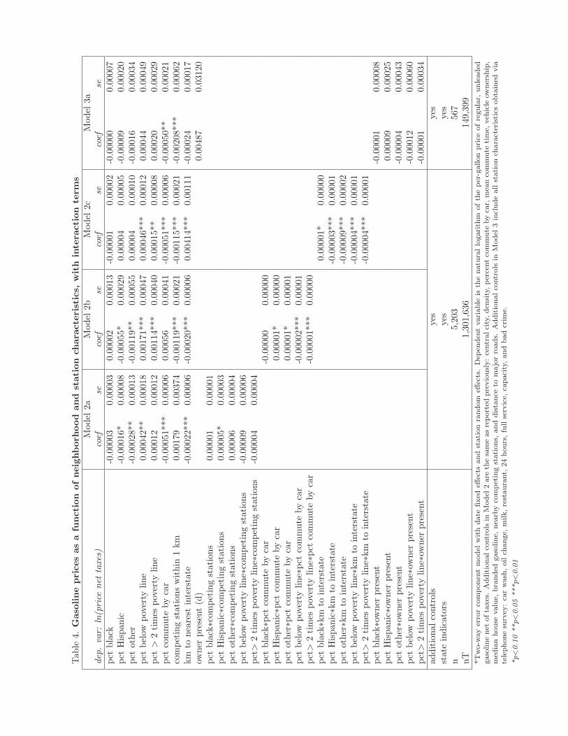
Explanations based on imperfect competition

A second possibility for the residual positive price differentials is that we have10Stations located near the boundary of the police district were dropped from the sample

because we could not observe crimes in the full 1 km radius around their locations.11Only 12 of the 116 stations were surveyed by telephone and, hence, have observations of

bad crime from the station survey to compare the crime rate obtained from the Atlanta PoliceDepartment. Of these stations with observations of both variables, the 9 stations reportingbad crime have a higher average crime rate (560 crimes) than the 3 stations that do not reportbad crime (507 crimes). The small sample size precludes testing for statistical significance.

12The full results are available upon request.

19

not fully observed lower levels of competition and/or relatively inelastic demand

for gasoline in poor and minority neighborhoods. For instance, residents of

poor, minority neighborhoods may be more likely to shop for goods other than

gasoline at gasoline stations, and may therefore be less responsive to the price

of gasoline.

If the residual income and racial price differentials are explained by imperfect

competition, we expect that they will be smaller in magnitude for stations that

have less market power. To investigate this possibility, we estimate Model 2 with

the addition of interactions between income composition and three variables

that relate to market power: competing stations within 1km, km to nearest

interestate, and pct commute by car. We expect that price discrimination will

be less likely when there is more competition as measured by the number of com-

peting stations and/or when demand is relatively elastic as measured by being

farther from an interstate or having more commuters in a neighborhood. Ac-

cordingly, when we observe positive price differentials in poor neighborhoods, we

expect the coefficients on interactions between the poverty rate and competing

stations within 1km, km to nearest interestate, and pct commute by car to

be negative. We also interact these variables will all three racial and ethnic cat-

egories. As with income, we expect the relationship between racial composition

and prices to be attenuated for stations with less market power.

Models 2a-2c in Table A present the estimated coefficients for interactions

between race and income and three variables measuring station competitive-

ness.13 As predicted, the estimated premiums paid in poor and middle-upper

income neighborhoods are smaller for more competitive stations in all three

models, although the differences are not always statistically significant. The

positive and statistically significant premium paid in neighborhoods with more13Separate estimates for the three metropolitan areas are available upon request. Overall,

they are consistent with the results for the pooled model: most of the estimated differentialsare attenuated for stations with less market power.

20

families in poverty decreases with the presence of competing stations (although

the interaction term is insignificant with a p-value of 0.16), with the percent

of residents who commute by car (p-value<0.01), and with distance from the

interstate (p-value<0.01). For instance, in Model 2a we estimate that the av-

erage gasoline premium for a 10 percentage point increase in the poverty rate

is 0.42 percent for stations with no nearby competitors (p-value= 0.02), but

0.24 percent for stations with 2 competitors within a one kilometer radius (p-

value= 0.02). In Model 2c we estimate that the average gasoline premium for a

10 percentage point increase in the poverty rate is 0.42 percent for stations that

are 1 km from an interstate (p-value< 0.01) and (a statistically insignificant)

0.26 percent for stations that are 5 km from an interstate (p-value= 0.90).

Similarly, we find that the positive premium paid with increasing middle-

upper income families also decreases with increased competition and with in-

creasing demand elasticity. The results for race are, again, mostly statistically

insignificant. However, the point estimates do suggest that racial price differ-

entials are attenuated in the presence of greater competition. For example, in

Model 2a we estimate that the average gasoline discount for a 10 percentage

point increase in the percent black is 0.03 percent for stations with no nearby

competitors (p-value= 0.28), but that the average discount is 0.01 percent for

stations with 2 nearby competitors (p-value= 0.82).

As a whole, these results are consistent with the explanation that the unex-

plained price differentials in poor and minority neighborhoods can be accounted

for by unobserved lower competition and/or less elastic demand.

Explanations based on animus-based price discrimination

A final possibility is that the unexplained inter-neighborhood price differentials

may reflect animus-based price discrimination on the basis of race or, in the

case of the income differentials, some factor associated with income that is

21

observable to station owners but not to us. If it is the case that the price

differentials result from animus-based discrimination related to race or income,

we expect that the differentials will be larger in magnitude at stations in which

the owner is routinely present and, hence, interacts with customers. Model 3a in

Table A reports estimated coefficients when racial and income characteristics are

interacted with the owner present indicator. Although the reduced sample size

in Model 3 again generates large standard errors and the coefficients of interest

are not statistically significant, we note that the point estimates are mixed.

The small and statistically insignificant discounts paid with increasing minority

composition (which would have to suggest animus-based discrimination against

whites) are more negative in the presence of owners in two of the three cases,

but still very small. The statistically significant premia paid in neighborhoods

with more poor or middle-upper income residents decrease in the presence of

station owners, which is not consistent with animus-based discrimination.

As a whole, the estimated racial and income price differentials do not behave

in a manner that is consistent with our predictions of the effects of animus-based

discrimination. However, like most Becker-type models, our theoretical model

allows animus-based discrimination to be maintained only if all stations have a

similar discrimination coefficient. If tastes for discrimination vary in a perfectly

competitive market, discriminating firms will go out of business. A second,

un-modeled, possibility is that tastes for discrimination vary and that firms in

less competitive markets are more likely to be able to engage in animus-based

discrimination without being priced out of business. In this case, the attenuated

price differentials observed at stations with more competition in Models 2a-2c

would be consistent with animus-based discrimination as well as with classic

price discrimination, and the two would not be separable.

22

7 Conclusion

We have introduced a large and unique data set to examine neighborhood vari-

ation in retail prices. Despite anecdotal evidence of higher prices in minority

neighborhoods, we estimate that any premiums paid for gasoline are quite small.

For instance, for a 10 percentage point increase in the black composition of a

Detroit or Philadelphia neighborhood, gasoline prices are estimated to increase

by about 0.05 percent, or by about 2 cents for a 15 gallon tank at the observed

mean price. The corresponding premium paid in Hispanic neighborhoods is

about 0.20 percent, or about 8 cents for a tank. Moreover, in Atlanta we find

evidence of discounts rather than a premium paid with minority composition,

although the magnitude of the discounts is similarly small.

Larger premia are observed in relation to income. On average across the

three cities in the data set, a 10 percentage point increase in poor relative to

lower-middle income families is associated with a 0.70 percent increase in gaso-

line prices. Two-thirds of this differential can be accounted for by the observable

cost, competition, and demand characteristics of poor neighborhoods. The re-

maining differential is again smaller for stations that have observably less market

power, suggesting that it may be explained by lower levels of competition and/or

more inelastic demand in poor neighborhoods.

We conclude that the evidence from the market for gasoline indicates that

prices are not greatly inflated in minority neighborhoods, but that there is a

small poverty premium that may represent a noteworthy burden for the very

poor living in very poor neighborhoods.

23

A Appendix: Station Telephone Survey Method-ology and Script

The telephone surveys of gasoline stations were conducted by undergraduate

students as part of a class research project. Students piloted an initial script

on approximately 100 stations. The students then worked together during an

afternoon workshop to refine the survey script based on their experience with the

pilot. The refinements included shortening the introduction and several of the

questions. The final version of the survey script is replicated below. Surveyors

reported that only a handful of respondents asked for more detailed information

on the nature of the survey.

Survey Script

First verify that you have the correct station. When the respondent answers thephone, if he or she identifies the station in some way that matches what youwere expecting, simply begin the script. If the respondent does not identify thestation, ask “Hi, is this the [brand] station on [street]?” If it is, continue.If it is not, say that you have the wrong number and hang up.

Then, ask the respondent if he or she is willing to complete the survey. Youcan say whatever feels comfortable, but try to keep it brief and clear. Somethinglike:

Hi, can I ask you a few questions for a class project? It will only takea minute.

Wait for response

• No: Thank them and hang up

• Ask you to call back: Record suggested time and call back as instructed

• Ask you for more information: Tell respondent that you are working ona research project on gasoline prices across neighborhoods. Answer allquestions briefly and truthfully.

• Yes: Proceed with Survey

Great! Thanks very much.

1. Does your station have a car wash?

24

2. Does your station perform oil changes?

3. Do you sell milk by the gallon?

4. Is there a restaurant like a McDonald’s that is part of yourstation?

5. Is your station open 24 hours a day?

6. Does your station pump the gas for customers?

(Question 6 excluded from surveys of New Jersey stations.)

7. How many cars can get gasoline at your station at the sametime?

8. On a scale of 1 to 10, how bad a problem would you say crimeis in your area?

9. Does the owner of your station also work behind the counter?

Thank you very much for you time.

25

References

Ian Ayres and Peter Siegelman. Race and gender discrimination in bargainingfor a new car. The American Economic Review, 85(3), June 1995.

Badi Baltagi. Econometric Analysis of Panel Data. John Wiley and Sons, Ltd,fourth edition, 2008.

Gary S. Becker. The Economics of Discrimination. University of Chicago Press,1957.

Timothy Bresnahan. Empirical studies of industries with market power. InRichard Schmalensee and Robert Willig, editors, Handbook of Industrial Or-ganization, volume 2. North-Holland, 1989.

DeNeen L. Brown. Poor? pay up. The Washington Post, May 18, 2009.

Roland Burris. Senator Roland W. Burris: FY2010 appropriations requests,April 29, 2009. Press Release.

Hayley Chouinard and Jeffrey Perloff. Incidence of federal and state gasolinetaxes. Economics Letters, 83(1), 2004.

Chanjin Chung and Samuel Myers. Do the poor pay more for food? an anal-ysis of grocery store availability and food price disparities. The Journal ofConsumer Affairs, 33(2), 1999.

City of Atlanta Police Department. 2007 crime data, downloaded February 24,2007. URL http://www.atlantapd.org/index.asp?nav=CrimeMapping.

Elizabeth Douglas and Gary Cohn. Zones of contention in gasoline pricing. TheLos Angeles Times, June 19, 2005.

David Downing. Driving shoppers to the suburbs. St. Paul Pioneer Press,March 13, 2007.

Denver D’Rozario and Jerome Williams. Retail redlining: Definition, theory,typology, and measurement. Journal of Macromarketing, 25(2), December2005.

Energy Information Administration. A primer on gasoline prices, 2009. URLhttp://www.eia.doe.gov/bookshelf/brochures/gasolinepricesprimer/.Informational brochure published by a division of the U.S. Department ofEnergy.

David Frankel and Eric Gould. The retail price of inequality. Journal of UrbanEconomics, 49(2), 2001.

Chevon Fuller. Service redlining: The new Jim Crow? Civil Rights Journal, 3(1), May 1998.

Georgia Department of Revenue. Motor fuel tax bulletins, 2007a.

Georgia Department of Revenue. Motor fuel tax bulletins, 2008.

26

Georgia Department of Revenue. Motor fuel tax bulletins, 2009.

Georgia Department of Revenue. Information bulletin #2007-12-19: House bill219– prepaid local tax on motor fuel, December 19, 2007b.

Uri Gneezy and John List. Are the disabled discriminated against in productmarkets? Evidence from field experiments. Working paper, 2004.

Pinelopi Koujianoi Goldberg. Dealer price discrimination in new car purchases:Evidence from the consumer expenditure survey. The Journal of PoliticalEconomy, 104(3), June 1996.

Kathryn Graddy. Do fast-food chains price discriminate on the race and incomecharacteristics of an area? Journal of Business and Economic Statistics, 15(4), 1997.

Bruce Hall. Neighborhood differences in retail food stores: Income versus raceand age of the population. Economic Geography, 59(3), 1983.

Lashawn Richburg Hayes. Do the poor pay more? An empirical investigationof price dispersion in food retailing. 2000.

Betsy Jelisavcic. When redlining isn’t; only banks and insurers are required to dobusiness in minority neighborhoods. The Cleveland Plain Dealer, November17, 1996.

Sheila Kaplan. The new face of racism. U.S. News and World Report, 128(1),January 1, 2000.

Phillip Kaufman, James MacDonald, Steve Lutz, and David Smallwood. Do thepoor pay more for food? Item selection and price differences affect low-incomehousehold food costs. Agricultural Economic Report 759, U.S. Departmentof Agriculture, 1997.

Andrew Kleit. The economics of gasoline retailing: Petroleum distribution andretailing issues in the U.S., December 2003. American Petroleum Institute.

John List. The nature and extent of discrimination in the marketplace: Evidencefrom the field. Quarterly Journal of Economics, 119(1), February 2004.

David Meyer and Jeffrey Fischer. The economics of price zones and territorialrestrictions in gasoline marketing, 2004. Federal Trade Commission workingpaper no. 271.

Caitlin Knowles Myers. Discrimination and neighborhood effects: Understand-ing racial differentials in U.S. housing prices. Journal of Urban Economics,56(2), September 2004.

Jan Ondrich, Stephen Ross, and John Yinger. Now you see it, now you don’t:Why do real estate agents withhold available houses from black customers?Review of Economics and Statistics, 85(4), November 2003.

John Pucher and John Renne. Socioeconomics of urban travel: Evidence fromthe 2001 NHTS. Transportation Quarterly, 57(3), 2003.

27

Craig Rose. Gasoline prices all over the map. San Diego Tribune, August 16,2007.

Amanda Shaffer. The persistence of l.a.’s grocery gap: The need for a new foodpolicy and approach to market development, 2002.

Andrea Shepard. Price discrimination and retail configuration. The Journal ofPolitical Economy, 99(1), 1991.

Peter Siegelman. Racial discriminationi in “everyday” commercial transactions:What do we know, what do we need to know, and how can we find out? InMichael Fix and Margery Austin Turner, editors, A National Report Card onDiscrimination in America: The Role of Testing. The Urban Institute, 1998.

Eric Smith. Caught red-handed? Civil rights group charges Wal-Mart withretail redlining. Black Enterprise, 26(10), May 1996.

Frederick Sturdivant. The Ghetto Marketplace. The Free Press, 1969.

Beck Taylor. Retail characteristics and ownership structure. Small BusinessEconomics, 14(2), 2000.

The American Petroleum Institute. State motor fuel excise and other taxes,January 12, 2009.

U.S. Department of Labor, Bureau of Labor Statistics. Consumer expendituresurvey, 2007 data tables, November 26, 2008.

John Yinger. Measuring discrimination with fair housing audits: Caught in theact. American Economic Review, 76(5), December 1986.

John Yinger. Closed Doors, Opportunities Lost: The continuing costs of housingdiscrimination. Russell Sage Foundation, 1995.

28

Table 1: Descriptive statistics for gasoline stations used in analysisFull Non-surveyed Surveyed

sample stations stationsVariable Source mean s.d. mean s.d. mean s.d.Outcomeprice OPIS 3.34 (0.16) 3.34 (0.16) 3.36 (0.12)price net taxes authors 2.86 (0.15) 2.86 (0.16) 2.86 (0.12)LocationMichigan (d) OPIS 0.31 (0.46) 0.30 (0.46) 0.36 (0.48)New Jersey (d) OPIS 0.07 (0.26) 0.07 (0.26) 0.05 (0.22)Pennsylvania (d) OPIS 0.18 (0.38) 0.18 (0.38) 0.22 (0.41)Georgia (d) OPIS 0.44 (0.50) 0.45 (0.50) 0.38 (0.49)central city (d) OPIS 0.17 (0.37) 0.17 (0.38) 0.13 (0.34)competing stations within 1 km ArcGIS 2.13 (1.37) 2.14 (1.37) 2.09 (1.39)km to nearest interstate ArcGIS 4.29 (4.92) 4.28 (4.84) 4.38 (5.51)km to nearest highway ArcGIS 5.13 (10.16) 4.95 (9.74) 6.55 (13.01)Census tract characteristicspct white Census 68.95 (30.18) 68.52 (30.37) 72.49 (28.35)pct black Census 21.39 (28.90) 21.79 (29.15) 18.16 (26.53)pct other Census 4.52 (4.17) 4.52 (4.18) 4.54 (4.13)pct Hispanic Census 5.13 (8.31) 5.17 (8.38) 4.81 (7.72)pct below poverty line Census 9.90 (9.30) 10.00 (9.45) 9.01 (7.96)pct 1 to 2 times poverty line Census 14.09 (7.55) 14.15 (7.54) 13.63 (7.57)pct > 2 times poverty line Census 76.01 (15.55) 75.85 (15.67) 77.36 (14.48)people/km2 Census 1301 (1620) 1317 (1649) 1176 (1348)pct commute by car Census 90.35 (9.38) 90.25 (9.55) 91.17 (7.81)avg commute time (minutes) Census 30.57 (5.08) 30.64 (5.08) 29.99 (5.00)pct of households with 1 vehicle Census 33.82 (10.98) 33.81 (10.98) 33.92 (16.84)pct of households with 2+ vehicles Census 57.02 (17.82) 56.97 (17.94) 57.41 (16.84)median house value Census 127,787 (65,197) 127,159 (65,159) 132,925 (65,338)Station characteristicsnumber of days in sample 250.17 (107.19) 248.54 (107.65) 263.49 (102.55)branded gasoline (d) OPIS 0.79 (0.40) 0.79 (0.41) 0.81 (0.39)car wash (d) survey 0.12 (0.33)oil change (d) survey 0.19 (0.39)milk (d) survey 0.75 (0.43)restaurant (d) survey 0.15 (0.36)24 hours (d) survey 0.45 (0.50)full service (d) survey 0.23 (0.42)capacity survey 9.20 (3.99)bad crime (d) survey 0.45 (0.50)owner present (d) survey 0.56 (0.50)n 5203 4636 567*Descriptive statistics for for all stations in analysis sample and by survey status. Price is the average price observed over theyear for a station. Dummy variables are noted by a (d).

29

Table 2: Gasoline price as a function of neighborhood and stationcharacteristics

Model 1 Model 2 Model 3dep. var: ln(price net taxes) coef se coef se coef seRace and income compositionpct black 0.00002 0.00001 -2.0x10−6 0.00002 -0.00001 0.00005pct Hispanic -0.00002 0.00004 -0.00004 0.00004 -0.00004 0.00013pct other 0.00007 0.00007 -0.00015** 0.00007 -0.00018 0.00022pct below poverty line 0.00070*** 0.00009 0.00022** 0.00010 0.00037 0.00033pct > 2 times poverty line 0.00048*** 0.00006 0.00002 0.00007 0.00020 0.00021Add’l neighborhoodcharacteristicscentral city (d) -0.00490*** 0.00108 -0.00660* 0.00340density (1,000 ppl/km2) -0.00056** 0.00027 -0.00010 0.00088pct commute by car -0.00051*** 0.00006 -0.00050** 0.00020avg commute time (minutes) -0.00009 0.00007 -0.00030 0.00023pct of households with 1 vehicle 0.00008 0.00008 0.00012 0.00021pct of households with 2+ vehicles 0.00002 0.00007 0.00003 0.00020ln(median house value) 0.01105*** 0.00104 0.00884*** 0.00314Station characteristicsbranded gasoline (d) 0.01410*** 0.00069 0.01568*** 0.00220competing stations within 1 km -0.00117*** 0.00021 -0.00210*** 0.00062km to nearest interstate -0.00021*** 0.00006 -0.00024 0.00017km to nearest highway 0.00009*** 0.00003 0.00014* 0.00007car wash (d) 0.00006 0.00254oil change (d) 0.00328 0.00259milk (d) 0.00017 0.00240restaurant (d) -0.00308 0.0023124 hours (d) 0.00127 0.00197full service (d) 0.00257 0.00224capacity -0.00015 0.00022badcrime 0.00075 0.00169owner present (d) 0.00295* 0.00169state indicators yes yes yesn 5,203 5,203 567nT 1,301,636 1,301,636 149,399*Two-way error component model with date fixed effects and station random effects. Dependent variable is the natural logarithm ofthe per-gallon price of regular, unleaded gasoline net of taxes.

*p<0.10 **p<0.05 ***p<0.01

30

Table 3: Gasoline price as a function of neighborhood characteristics,by metropolitan area

Model 1 Model 2dep. var: ln(price net taxes) coef se coef seAtlantapct black -3.1x10−6 0.00002 -0.00004* 0.00002pct Hispanic -0.00002 0.00006 -0.00018*** 0.00007pct other 0.00011 0.00012 0.00001 0.00012pct below poverty line 0.00069*** 0.00014 0.00010 0.00016pct > 2 times poverty line 0.00023*** 0.00008 -0.00015 0.00011Detroitpct black 0.00003* 0.00002 0.00005** 0.00002pct Hispanic 0.00008 0.00006 0.00018*** 0.00006pct other 0.00039*** 0.00010 0.00020* 0.00010pct below poverty line 0.00065*** 0.00012 0.00026** 0.00013pct > 2 times poverty line 0.00062*** 0.00008 0.00012 0.00009Philadelphiapct black 0.00014*** 0.00004 0.00007* 0.00004pct Hispanic -0.00005 0.00011 0.00022** 0.00011pct other -0.00008 0.00016 -0.00050*** 0.00015pct below poverty line 0.00146*** 0.00024 0.00075*** 0.00025pct > 2 times poverty line 0.00113*** 0.00014 0.00064*** 0.00016additional controls no yes*Two-way error component model with date fixed effects and station random effects. De-pendent variable is the natural logarithm of the per-gallon price of regular, unleaded gasolinenet of taxes. Additional controls in Model 2 are the same as reported previously: central city,density, percent commute by car, mean commute time, vehicle ownership, median house value,branded gasoline, nearby competing stations, and distance to major roads. State indicatorsare not included for the Atlanta and Detroit metropolitan areas, which are each contained inone state, but a New Jersey indicator is included in both models for Philadelphia.

*p<0.10 **p<0.05 ***p<0.01

31

Tab

le4.

Gas

olin

epri

ces

asa

funct

ion

ofnei

ghbor

hood

and

stat

ion

char

acte

rist

ics,

with

inte

ract

ion

term

sM

odel

2aM

odel

2bM

odel

2cM

odel

3ade

p.va

r:ln

(pri

cene

tta

xes)

coef

seco

efse

coef

seco

efse

pct

blac

k-0

.000

030.

0000

30.

0000

20.

0001

3-0

.000

010.

0000

2-0

.000

000.

0000

7pc

tH

ispa

nic

-0.0

0016

*0.

0000

8-0

.000

55*

0.00

029

0.00

004

0.00

005

-0.0

0009

0.00

020

pct

othe

r-0

.000

28**

0.00

013

-0.0

0119

**0.

0005

50.

0000

40.

0001

0-0

.000

160.

0003

4pc

tbe

low

pove

rty

line

0.00

042*

*0.

0001

80.

0017

1***

0.00

047

0.00

046*

**0.

0001

20.

0004

40.

0004

9pc

t>

2ti

mes

pove

rty

line

0.00

012

0.00

012

0.00

114*

**0.

0004

00.

0001

5**

0.00

008

0.00

020

0.00

029

pct

com

mut

eby

car

-0.0

0051

***

0.00

006

0.00

056

0.00

041

-0.0

0051

***

0.00

006

-0.0

0050

**0.

0002

1co

mpe

ting

stat

ions

wit

hin

1km

0.00

179

0.00

374

-0.0

0119

***

0.00

021

-0.0

0115

***

0.00

021

-0.0

0208

***

0.00

062

kmto

near

est

inte

rsta

te-0

.000

22**

*0.

0000

6-0

.000

20**

*0.

0000

60.

0041

4***

0.00

111

-0.0

0024

0.00

017

owne

rpr

esen

t(d

)0.

0048

70.

0312

0pc

tbl

ack∗

com

peti

ngst

atio

ns0.

0000

10.

0000

1pc

tH

ispa

nic∗

com

peti

ngst

atio

ns0.

0000

5*0.

0000

3pc

tot

her∗

com

peti

ngst

atio

ns0.

0000

60.

0000

4pc

tbe

low

pove

rty

line∗

com

peti

ngst

atio

ns-0

.000

090.

0000

6pc

t>2

tim

espo

vert

ylin

e∗co

mpe

ting

stat

ions

-0.0

0004

0.00

004

pct

blac

k∗pc

tco

mm

ute

byca

r-0

.000

000.

0000

0pc

tH

ispa

nic∗

pct

com

mut

eby

car

0.00

001*

0.00

000

pct

othe

r∗pc

tco

mm

ute

byca

r0.

0000

1*0.

0000

1pc

tbe

low

pove

rty

line∗

pct

com

mut

eby

car

-0.0

0002

***

0.00

001

pct>

2ti

mes

pove

rty

line∗

pct

com

mut

eby

car

-0.0

0001

***

0.00

000

pct

blac

k∗km

toin

ters

tate

0.00

001*

0.00

000

pct

His

pani

c∗km

toin

ters

tate

-0.0

0003

***

0.00

001

pct

othe

r∗km

toin

ters

tate

-0.0

0009

***

0.00

002

pct

belo

wpo

vert

ylin

e∗km

toin

ters

tate

-0.0

0004

***

0.00

001

pct>

2ti

mes

pove

rty

line∗

kmto

inte

rsta

te-0

.000

04**

*0.

0000

1pc

tbl

ack∗

owne

rpr

esen

t-0

.000

010.

0000

8pc

tH

ispa

nic∗

owne

rpr

esen

t0.

0000

90.

0002

5pc

tot

her∗

owne

rpr

esen

t-0

.000

040.

0004

3pc

tbe

low

pove

rty

line∗

owne

rpr

esen

t-0

.000

120.

0006

0pc

t>2

tim

espo

vert

ylin

e∗ow

ner

pres

ent

-0.0

0001

0.00

034

addi

tion

alco

ntro

lsye

sye

sst

ate

indi

cato

rsye

sye

sn

5,20

356

7nT

1,30

1,63

614

9,39

9*T

wo-w

ay

erro

rco

mponen

tm

odel

wit

hdate

fixed

effec

tsand

stati

on

random

effec

ts.

Dep

enden

tvari

able

isth

enatu

rallo

gari

thm

ofth

eper

-gallon

pri

ceofre

gula

r,unle

aded

gaso

line

net

ofta

xes

.A

ddit

ionalco

ntr

ols

inM

odel

2are

the

sam

eas

report

edpre

vio

usl

y:

centr

alci

ty,den

sity

,per

cent

com

mute

by

car,

mea

nco

mm

ute

tim

e,veh

icle

ow

ner

ship

,m

edia

nhouse

valu

e,bra

nded

gaso

line,

nea

rby

com

pet

ing

stati

ons,

and

dis

tance

tom

ajo

rro

ads.

Addit

ionalco

ntr

ols

inM

odel

3in

clude

all

stati

on

chara

cter

isti

csobta

ined

via

tele

phone

surv

ey:

car

wash

,oil

change,

milk,re

staura

nt,

24

hours

,fu

llse

rvic

e,ca

paci

ty,and

bad

crim

e.

*p<

0.1

0**p<

0.0

5***p<

0.0

1