return and volatility spillovers from developed markets to
TRANSCRIPT
Return and Volatility Spillovers from Developed to Emerging Capital Markets: The Case of South Asia
Yun Wang#, Abeyratna Gunasekarage## and David M. Power###
#Performance Group, Commerce Commission, Level 6, 44-52 Terrace, PO Box 2351, Wellington, New Zealand. Phone 0064 4 924 3648, Fax 0064 4 924 3700, E-mail:[email protected]. ##Department of Finance, Waikato Management School, University of Waikato, Private Bag 3105, Hamilton, New Zealand. Phone: 0064-7-858 5082; Fax: 0064-7-838 4331; E-mail: [email protected]. ###Department of Accountancy and Business Finance, University of Dundee, Dundee DD1 4HN, Scotland, UK. Phone: 0044-1382 344854; Fax: 0044-1382 344193; E-mail: [email protected].
Abstract
This study examines return and volatility spillovers from the US and Japanese stock markets to three South Asian capital markets – (i) the Bombay Stock Exchange, (ii) the Karachi Stock Exchange, and (iii) the Colombo Stock Exchange. We construct a univariate EGARCH spillover model which allows the unexpected return of any particular South Asian market to be driven by a local shock, a regional shock from Japan, and a global shock from the USA. The study discovers return spillovers in all three markets, and volatility spillovers from the US to the Indian and Sri Lankan markets, and from the Japanese to the Pakistani market. Regional factors seem to exert an influence on these three markets before the Asian financial crisis but the global factor becomes more important in the post-crisis period. JEL Classification: G14; G15 Key Words: Integration; Spillover; EGARCH Model; Asymmetric Effect.
I. Introduction
The theme of integration among international capital markets and the
mechanism whereby information is transmitted among different stock exchanges has
been extensively researched in the modern finance literature. This topic has attracted
the attention of financial economists as the turmoils which occur in some capital
markets have far reaching consequences on security prices on their counterparts in
other countries. For example, the October 1987 crash not only eliminated more than
20 per cent of the market value of US equities but also sent shock waves around the
world. The Asian financial crisis had a similar impact on many other emerging
markets in Latin America as well as in Eastern Europe. The liberalization of capital
movements together with advances in computer technology and the improved world-
wide processing of news have improved the possibilities for national financial markets
to react rapidly to new information from international stock exchanges.
Early investigations in this area analysed the interrelatedness among developed
capital markets using correlations of stock returns. For example, Hilliard (1979)
examined indices for ten international equity markets (Amsterdam, Frankfurt,
London, Milan, New York, Paris, Sydney, Tokyo, Toronto, and Zurich) during the
world-wide financial crisis created by the OPEC embargo in the period of 1973-1974
and found that the most intra-continental prices move simultaneously. More recently,
Eun and Shim (1989) applied vector autoregression (VAR) methodology to study
daily index data for nine of the largest stock exchanges in the world (Australia,
Canada, France, Germany, Hong Kong, Japan, Switzerland, the UK, and the US) and
discovered a substantial amount of multi-lateral interaction among these markets; the
US stock market was the most influential and none of the other markets explained any
movements in US returns. Joen and von Furstenberg (1990) arrived at a similar view;
2
they highlighted evidence of growing international integration among the four major
equity markets of Germany, Japan, the UK and the US in the 1980s. Becker et al.
(1990) concluded that the information from the US market could be used to trade
profitably in the Japanese market as there was a high correlation between the open-to-
close returns of US shares in the previous trading day and the returns of Japanese
equities in the current period. Koch and Koch (1991), who used a dynamic
simultaneous equations model to investigate the contemporaneous and lead-lag
relationships among eight national stock exchanges (Australia, Germany, Hong Kong,
Japan, Singapore, Switzerland, the UK, and the US), discovered a growing level of
market interdependence within the same geographical regions over time; an
increasing influence of the Japanese market at the expense of the US market was also
detected.
Another branch of research concentrates on the transmission of international
equity movements by studying the spillover of return and volatility across markets.
For example, Hamao et al. (1990), who studied three major stock markets (London,
New York and Tokyo,) using univariate GARCH-in-mean models, found volatility
spillovers (i) from New York to Tokyo and London and (ii) from London to Tokyo.
Theodossiou and Lee (1993) used multivariate GARCH-in-mean models to analyse
the markets in Canada, Germany, Japan, the UK and the US; they discovered that the
US market was the major exporter of volatility. More recently, Scheicher (2001)
analysed three Eastern European markets (Czech Republic, Hungary and Poland) and
reported that although the equity returns were affected by both regional and global
factors, the volatilities were impacted by only regional influences. Fratzscher (2002)
and Baele (2002) arrived at a similar conclusion; they documented evidence that
3
shock transmissions from the aggregate European Union market to domestic
European equities had become more pronounced in recent years1.
A number of researchers have addressed the question of whether the quantity of
news (i.e. the size of an innovation) and the quality of the information (i.e. the sign of
an innovation) are important determinants of the degree of volatility spillover across
markets. This question has been motivated by findings of an ‘asymmetric’ or
‘leverage’ effect associated with equity returns; bad news has a different degree of
predictability on future volatility compared to its good news counterpart2. This
asymmetric effect has been examined in studies of volatility spillovers across markets.
For example, Bae and Karolyi (1994), who examined the joint dynamics of overnight
and daytime return volatility for the New York and Tokyo stock markets over the
period 1988-1992, noted that the magnitude and persistence of shocks originating in
New York or Tokyo that transmitted to the other market were significantly
understated if this asymmetric effect was ignored; bad news from domestic and
foreign markets appeard to have a much larger impact on subsequent return volatility
than good news. Koutmos and Booth (1995) investigated the asymmetric impact of
market advances and market declines (i.e. good and bad news respectively) on
volatility transmission across the New York, Tokyo and London stock markets. Using
daily open-to-close returns, they found unidirectional price spillovers (i) from New
York to Tokyo, (ii) from New York to London, and (iii) from Tokyo to London. They
also uncovered bidirectional volatility spillovers among the three markets. In all
1 Some researchers have extended this investigation to foreign exchange and spot and future markets and uncovered evidence for the existence of spillovers among major currency markets (Baillie and Bollerslev, 1990; Engle et al., 1991; Chin et al., 1991; Cheung and Fung, 1997). 2 This phenomenon was originally motivated by the work of Black (1976), Christie (1982), French et al. (1987) and Nelson (1991) and its significance was evaluated by Pagan and Schwert (1990), Braun et al. (1992), Glosten et al. (1993) and Engle and Ng (1993) by employing different variations of volatility models. Nelson (1991), Cheung and Ng (1992), Koutmos (1992) and Poon and Taylor (1992), among others, provide empirical evidence for the existence of a leverage effect.
4
instances, the volatility transmission mechanism was asymmetric - i.e. negative
innovations in one market increased volatility in the other market considerably more
than their positive counterparts. Booth et al. (1997) looked at the four Scandinavian
markets and found significant and asymmetric volatility spillovers among Swedish,
Danish, Norwegian, and Finnish securities. Similar evidence has been reported for
other European markets - London, Paris, and Frankfurt – by Kanas (1998).
Only a minority of studies have focussed on the return and volatility spillovers
from developed to emerging capital markets3. In particular, the evidence on market
interactions and information transmissions in South Asian capital markets is hard to
find. The Capital markets in South Asia have generated a considerable interest among
local and foreign investors as a result of the increased economic activity in these
countries arising from economic reforms and the liberalisation of capital markets. In
this research exercise, we investigate how information is transmitted from developed
capital markets to three recently libaralised South Asian capital markets – the Bombay
Stock Exchange (BSE) of India, the Karachi Stock Exchange (KSE) of Pakistan and
the Colombo Stock Exchange (CSE) of Sri Lanka; return and volatility spillover
models are tested on market index data. Our study differs from the previous research
on this topic in three respects. First, unlike many existing studies which focus on how
a single international market (often the US or a world market) influences other stock
markets4, we consider the innovations from both the US and Japanese markets in an
attempt to analyse the impacts of both regional and world shocks on South Asian
equities. Second, we recognise that volatility transmission may be asymmetric in
3 See, Ng (2000), Chan-Lau and Ivaschenko (2002) and Worthington and Higgs (2004) for some evidence on this topic. 4 Many early studies failed to distinguish between world and regional factors as they were predominantly occupied with testing the influence of the world market (often US) on other markets. For example, see Hamao et al. (1990), Campbell and Hamao (1992), Bekaert and Hodrick (1992), Bekaert and Harvey (1995), Harvey (1995), Karolyi (1995) and Karolyi and Stulz (1996).
5
character – i.e. the negative innovations in one market may produce higher volatility
spillovers in another market, than the positive innovations of equal magnitude.
Finally, we address the possible effect of the Asian financial crisis5 on the
transmission mechanism by disaggregating the data into three sample periods: (i) pre-
crisis, (ii) in-crisis and (iii) post-crisis.
The reminder of this paper is organized as follows. Section II provides a brief
overview about the South Asian stock markets. Section III describes the spilover
models used to analyse the data in this study. Section IV outlines the data employed in
the study and presents the empirical results. The final section offers some conclusions.
II. An Overview of South Asian Capital Markets
The South Asian region is notable for its large population (more than one-fifth
of the world total’s inhibitants) which continues to grow rapidly. India is by far the
largest South Asian country, in terms of population, GDP, and land area. Sri Lanka
has the most open economy. Indian, Pakistan, and Sri Lankan stock exchanges are
also the three biggest markets in this region in terms of market capitalization. South
Asia has experienced fast economic growth in recent years because of the economic
reforms implemented by these countries’ governments; it was the fastest growing
region of the world in 1998. The emerging capital markets in this region have
generated considerable interest among regional as well as global investors because of
the rapid growth of these countries’ economies and the concessions provided to
foreign investors through radical liberalization processes.
The Bombay Stock Exchange is the oldest stock market in Asia - even older
than the Tokyo Stock Exchange - and was established in 1875 as a voluntary non-
5 Bollerslev et al. (1992) suggest that the asymmetric response of volatility to innovations may be the
6

profit making association. It is one of 25 stock markets throughout India. With over
20 million shareholders, India has the third largest investor base in the world after the
US and Japan. India's market capitalization was the 6th highest among the emerging
markets. Share trading on Colombo Stock Exchange dates back to the 19th century; in
1896 Colombo Brokers Association commenced the trading of shares in limited
liability companies. By contrast, the stock market in Pakistan is relatively new. The
Karachi Stock Exchange only came into existence in 1947. These capital markets
exhibit a number of common features; they did not play a prominent role in the
economic development of their countries until the respective governments started a
programme of deregulation and economic liberalization. For example, India initiated
financial reforms in conjunction with economic deregulation and permitted foreign
companies to own a majority stake in quoted Indian firms from many different
industries. The liberalization policies of the Pakistan government have led to rapid
deregulation of the economy and the removal of impediments to private investment.
The secondary stock market in Pakistan is now open to foreign investors; non-
nationals are treated equally with local participants when trading shares. The Sri
Lankan government took a number of steps including the opening of the banking
sector to foreign owners, repealing the business acquisition act and privatizing
government-owned business undertakings in an attempt to create a well-functioning
capital market in the country.
TABLE 1 ABOUT HERE
result of a few extreme observations such as those associated with the October 1987 crash.
7

As a result of these changes, share markets in these three South Asian
countries recorded a remarkable rate of growth in their trading activities. Table 1
reports some market statistics for the stock exchanges in these countries. According to
this table, during the 10-year period ending 2003, these markets have reported a
phenomenal growth in market capitalization: BSE 341.93 per cent, KSE 1,268.57 per
cent and CSE 112.10 per cent. Similar growth patterns can be observed with respect
to market capitalization as a percentage of GDP, annual turnover, the number of listed
companies, and the market price index. The number of companies listed on the BSE at
the end of December 1998 was 5,860. This was more than the aggregate total of
companies listed in 9 emerging markets (Malaysia, South Africa, Mexico, Taiwan,
Korea, Philippines, Thailand, Brazil and Chile) at the same date. The number of listed
companies was also larger than that in several developed markets: Japan, UK,
Germany, France, Australia, Switzerland, Canada and Hong Kong. The KSE has also
grown quickly, especially in recent years. It was declared the “best performing stock
market of the World for the year 2002” by Business Week. The findings of this study
will be interesting as little evidence appears in the finance literature on South Asian
capital markets.
III. Methodology
EGARCH Model Estimation
GARCH (generalized autoregressive conditional heteroskedasticity) models
are generally used to explore the stochastic behavior of several financial time series
and, in particular, to explain the behavior of volatility over time. However, such
models do not work with negative data. The exponential GARCH (EGARCH) model
8
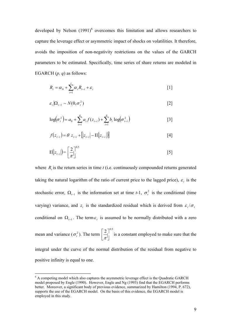
developed by Nelson (1991)6 overcomes this limitation and allows researchers to
capture the leverage effect or asymmetric impact of shocks on volatilities. It therefore,
avoids the imposition of non-negativity restrictions on the values of the GARCH
parameters to be estimated. Specifically, time series of share returns are modeled in
EGARCH (p, q) as follows:
∑=
− ++=r
ititit RR
10 εαα [1]
),0(~ 21 ttt N σε −Ω [2]
( ) (∑∑=
−=
− ++=p
iiti
q
iitit bzfaa
1
2
10
2 log)(log σσ ) [3]
( ) θ=−itzf ( )[ ititit zzz −−− Ε−+ ] [4]
( )itz −Ε = 5.02
π
[5]
where is the return series in time t (i.e. continuously compounded returns generated
taking the natural logarithm of the ratio of current price to the lagged price),
tR
tε is the
stochastic error, is the information set at time t-1, is the conditional (time
varying) variance, and is the standardized residual which is derived from
1−Ωt2tσ
tz tε /
conditional on . The term
tσ
1−Ωt tε is assumed to be normally distributed with a zero
mean and variance ( ). The term 2tσ
5.02
π
is a constant employed to make sure that the
integral under the curve of the normal distribution of the residual from negative to
positive infinity is equal to one.
6 A competing model which also captures the asymmetric leverage effect is the Quadratic GARCH model proposed by Engle (1990). However, Engle and Ng (1993) find that the EGARCH performs better. Moreover, a significant body of previous evidence, summarized by Hamilton (1994, P. 672), supports the use of the EGARCH model. On the basis of this evidence, the EGARCH model is employed in this study.
9
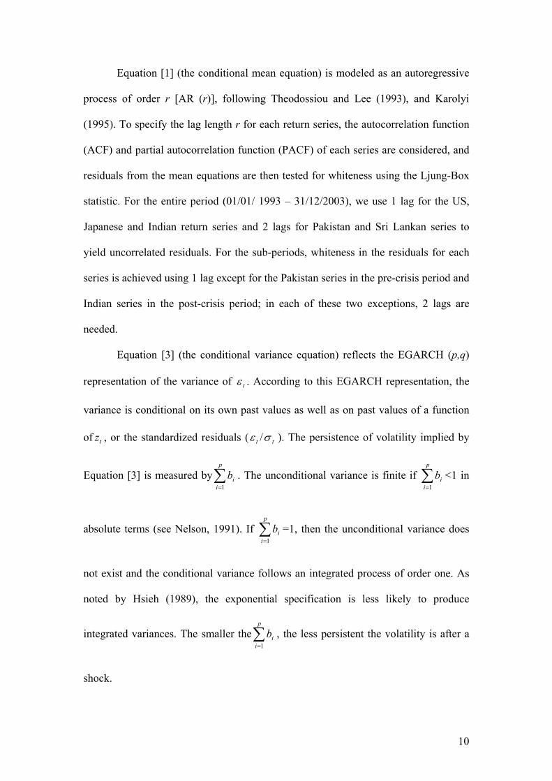
Equation [1] (the conditional mean equation) is modeled as an autoregressive
process of order r [AR (r)], following Theodossiou and Lee (1993), and Karolyi
(1995). To specify the lag length r for each return series, the autocorrelation function
(ACF) and partial autocorrelation function (PACF) of each series are considered, and
residuals from the mean equations are then tested for whiteness using the Ljung-Box
statistic. For the entire period (01/01/ 1993 – 31/12/2003), we use 1 lag for the US,
Japanese and Indian return series and 2 lags for Pakistan and Sri Lankan series to
yield uncorrelated residuals. For the sub-periods, whiteness in the residuals for each
series is achieved using 1 lag except for the Pakistan series in the pre-crisis period and
Indian series in the post-crisis period; in each of these two exceptions, 2 lags are
needed.
Equation [3] (the conditional variance equation) reflects the EGARCH (p,q)
representation of the variance of tε . According to this EGARCH representation, the
variance is conditional on its own past values as well as on past values of a function
of , or the standardized residuals (tz tε / ). The persistence of volatility implied by
Equation [3] is measured by . The unconditional variance is finite if <1 in
absolute terms (see Nelson, 1991). If =1, then the unconditional variance does
not exist and the conditional variance follows an integrated process of order one. As
noted by Hsieh (1989), the exponential specification is less likely to produce
integrated variances. The smaller the∑ , the less persistent the volatility is after a
shock.
tσ
∑=
p
ib1
ib
∑=
p
iib
1∑=
p
iib
1
i
=
p
i 1
10
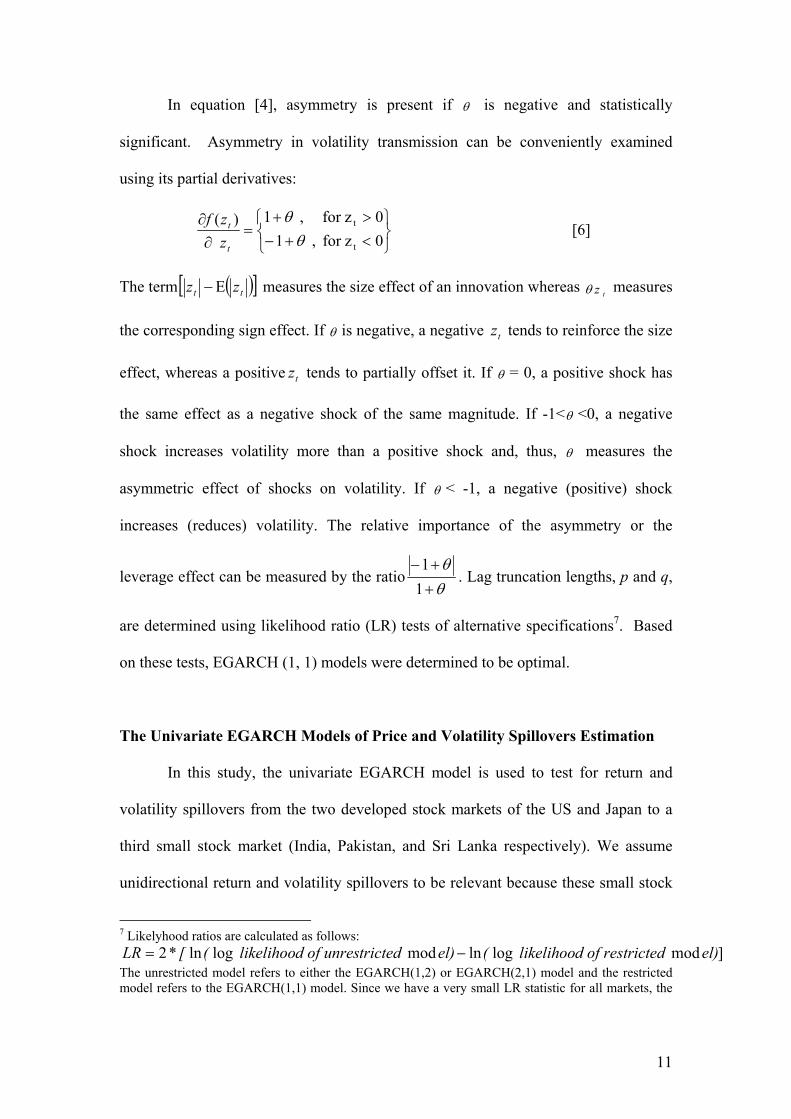
In equation [4], asymmetry is present if θ is negative and statistically
significant. Asymmetry in volatility transmission can be conveniently examined
using its partial derivatives:
<+−>+
=∂∂
0zfor ,10zfor ,1)(
t
t
θθ
t
t
zzf
[6]
The term ( )tt zz Ε−[ measures the size effect of an innovation whereas ]tzθ measures
the corresponding sign effect. If θ is negative, a negative tends to reinforce the size
effect, whereas a positive tends to partially offset it. If
tz
tz θ = 0, a positive shock has
the same effect as a negative shock of the same magnitude. If -1<θ <0, a negative
shock increases volatility more than a positive shock and, thus, θ measures the
asymmetric effect of shocks on volatility. If θ < -1, a negative (positive) shock
increases (reduces) volatility. The relative importance of the asymmetry or the
leverage effect can be measured by the ratioθθ+
+
−
11
. Lag truncation lengths, p and q,
are determined using likelihood ratio (LR) tests of alternative specifications7. Based
on these tests, EGARCH (1, 1) models were determined to be optimal.
The Univariate EGARCH Models of Price and Volatility Spillovers Estimation
In this study, the univariate EGARCH model is used to test for return and
volatility spillovers from the two developed stock markets of the US and Japan to a
third small stock market (India, Pakistan, and Sri Lanka respectively). We assume
unidirectional return and volatility spillovers to be relevant because these small stock
7 Likelyhood ratios are calculated as follows:
]modloglnmodlogln*2 el)icted d of restr likelihoo(el)tricted d of unres likelihoo([LR −=The unrestricted model refers to either the EGARCH(1,2) or EGARCH(2,1) model and the restricted model refers to the EGARCH(1,1) model. Since we have a very small LR statistic for all markets, the
11
markets are not thought to have a substantial impact on the two developed markets
considered. To test for spillovers from a foreign market to the domestic market, the
approach adopted by Hamao et al. (1990) and Theodossiou and Lee (1993) is
followed. According to this approach, the most recent squared residuals from the
conditional mean–conditional variance formulation of the foreign market are
introduced as an exogenous variable in the conditional variance equation of the
domestic market. The univariate EGARCH (1, 1) models of return and volatility
spillovers for market j are specified as follows:
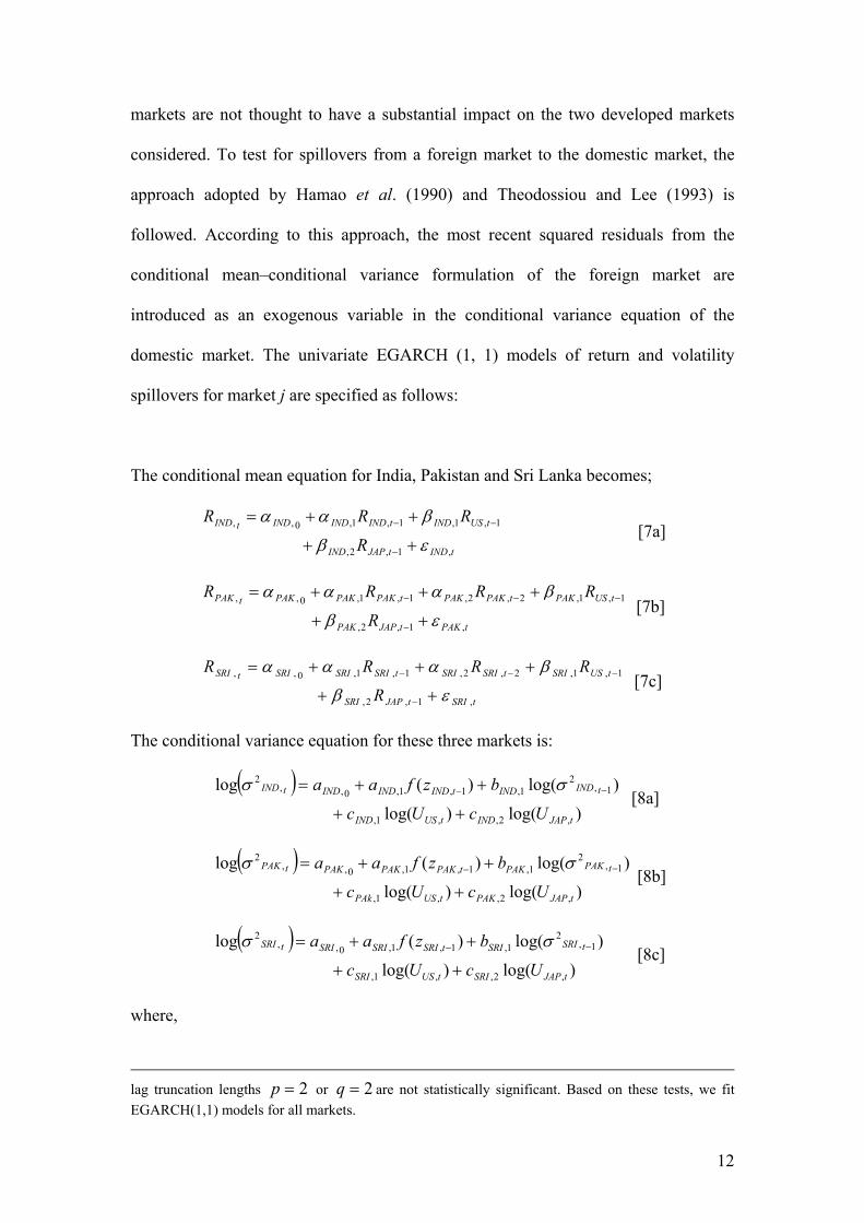
The conditional mean equation for India, Pakistan and Sri Lanka becomes;
tINDtJAPIND
tUSINDtINDINDINDtIND
R
RRR
,1,2,
1,1,1,1,0,,
εβ
βαα
++
++=
−
−− [7a]
tPAKtJAPPAK
tUSPAKtPAKPAKtPAKPAKPAKtPAK
R
RRRR
,1,2,
1,1,2,2,1,1,0,,
εβ
βααα
++
+++=
−
−−− [7b]
tSRItJAPSRI
tUSSRItSRISRItSRISRISRItSRI
R
RRRR
,1,2,
1,1,2,2,1,1,0,,
εβ
βααα
++
+++=
−
−−− [7c]
The conditional variance equation for these three markets is:
( ))log()log(
)log()(log
,2,,1,
1,2
1,1,1,0,,2
tJAPINDtUSIND
tINDINDtINDINDINDtIND
UcUc
bzfaa
++
++= −− σσ [8a]
( ))log()log(
)log()(log
,2,,1,
1,2
1,1,1,0,,2
tJAPPAKtUSPAk
tPAKPAKtPAKPAKPAKtPAK
UcUc
bzfaa
++
++= −− σσ [8b]
( ))log()log(
)log()(log
,2,,1,
1,2
1,1,1,0,,2
tJAPSRItUSSRI
tSRISRItSRISRISRItSRI
UcUc
bzfaa
++
++= −− σσ [8c]
where,
2=p 2=qlag truncation lengths or are not statistically significant. Based on these tests, we fit
EGARCH(1,1) models for all markets.
12
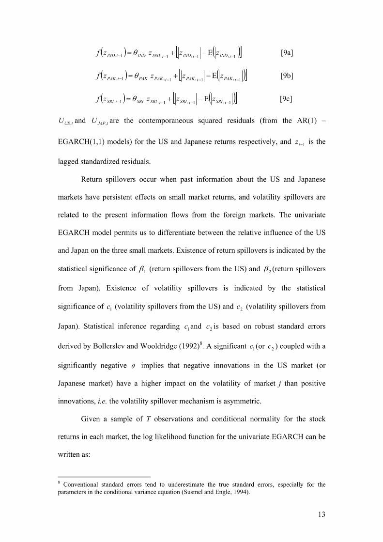
( ) INDtINDzf θ=−1, ( )[ ]1,1,1, −−−
Ε−+tINDtINDtIND zzz [9a]
( ) PAKtPAKzf θ=−1, ( )[ ]1,1,1, −−−
Ε−+tPAKtPAKtPAK zzz [9b]
( ) SRItSRIzf θ=−1, ( )[ ]1,1,1, −−−
Ε−+tSRItSRItSRI zzz [9c]
tUSU , and are the contemporaneous squared residuals (from the AR(1) –
EGARCH(1,1) models) for the US and Japanese returns respectively, and is the
lagged standardized residuals.
tJAPU ,
1−tz
Return spillovers occur when past information about the US and Japanese
markets have persistent effects on small market returns, and volatility spillovers are
related to the present information flows from the foreign markets. The univariate
EGARCH model permits us to differentiate between the relative influence of the US
and Japan on the three small markets. Existence of return spillovers is indicated by the
statistical significance of 1β (return spillovers from the US) and 2β (return spillovers
from Japan). Existence of volatility spillovers is indicated by the statistical
significance of c (volatility spillovers from the US) and (volatility spillovers from
Japan). Statistical inference regarding and is based on robust standard errors
derived by Bollerslev and Wooldridge (1992)
1 2c
1c 2c
8. A significant c (or c ) coupled with a
significantly negative
1 2
θ implies that negative innovations in the US market (or
Japanese market) have a higher impact on the volatility of market j than positive
innovations, i.e. the volatility spillover mechanism is asymmetric.
Given a sample of T observations and conditional normality for the stock
returns in each market, the log likelihood function for the univariate EGARCH can be
written as:
8 Conventional standard errors tend to underestimate the true standard errors, especially for the parameters in the conditional variance equation (Susmel and Engle, 1994).
13

∑=
−−=ΘT
ttTL
1
2 )log(5.0)2log()2/()( σπ [10]
where Θ is the parameter vector ( 0α 1α 2α 0a 1a 1b 1c 2c θ ) to be estimated.
IV. Empirical Findings
Data and Preliminary Statistics
The data used in the study consist of daily stock indices for five countries - the
USA, Japan, India, Pakistan, and Sri Lanka for the period 1 January 1993 to 31
December 2003; a total of 2869 observations are employed for each market. The
sample period is divided into three sub-periods – pre-crisis (01/01/1993- 31/06/1997),
in-crisis (01/07/1997-31/12/1999), and post-crisis (01/01/2000-31/12/2003). The
index data are obtained from Datastream. The stock market indices used in this study
are the S&P 500 (the US), the Nikkei 500 (Japan), the BSE National Price Index
(India), the Karachi 100 Price Index (Pakistan), and the Colombo All Share Price
Index (Sri Lanka). In each market, we choose the most comprehensive and diversified
stock index. The S&P 500 index consists of the 500 largest, publicly-held companies
representing approximately 76 percent of total market capitalization. The Nikkei 500
index incorporates 500 Japanese companies listed in the First Section of the Tokyo
Stock Exchange. The BSE National Index comprises 100 stocks listed at five major
Indian stock exchanges (Mumbai, Calcutta, Delhi, Ahmedabad and Madras). The
Karachi 100 includes the largest 100 companies in the exchange (27 companies
representing 27 sectors and 73 companies representing the entire market) covering
about 83 percent of market capitalization of the exchange. The Colombo All Share
14

Price Index consists of all the shares traded on the stock exchange9.With the exception
of the Nikkei 500, all indices are calculated on a value-weighted basis. The Japanese
index is a share price-weighted index which does not take dividend reinvestment into
account. However, cash dividends paid on most Japanese stocks are relatively small,
so this dividend omission is of little consequence. 10 The variable analysed in the
study is the daily return which is calculated by taking the natural logarithm of the ratio
of current price to the lagged price11.
TABLE 2 ABOUT HERE
Table 2 reports summary statistics for the daily returns of the five national
stock markets. The mean returns are positive for four markets with the exception of
Japan. The Pakistan market earned the highest mean return but with the largest risk as
measured by the standard deviation. However, the sample means for all five markets
are not statistically different from zero. The measures for skewness show that with the
exception of the distribution of returns for the Sri Lankan market, the return series are
negatively skewed. The excess Kurtosis measures indicate that the distributions of all
the return series are highly leptokurtic. Likewise, the Jarque-Bera statistics reject
normality for each of the return series at the 1 percent level of significance.
The Ljung-Box q-statistics - LB(k) and LB2(k) - for lag lengths of 6 and 12
days are used to test for serial correlation in the return and squared return series. The
9 Even though the CSE had a “blue chips” index representing the top companies in the market, its composition changed in 1998. Therefore, it was decided to use the All Share Price Index. 10 See Campbell and Hamao (1989) for evidence on the dividend-price ratio for the Tokyo market. 11 Since Eastern trading time leads Western trading time by one day, we consider US returns with a one day lag in order to overcome problems associated with non-synchroneous trading across five markets analysed. All three South Asian markets have overlapping trading hours with the Japanese market but not with the US market. Recent spillover investigations deal with this problem using open-to-close returns (Hamao et al. 1990; Bae and karolyi, 1994; and Koutmos and Booth, 1995). However, this
15

null hypothesis of uncorrelated returns is rejected at the 1 percent level of significance
for the markets of Japan, India, Pakistan, and Sri Lanka at both lag lengths used. The
null hypothesis of homoskedastic returns (uncorrelated squared returns) is also
rejected at the 1 percent level for all markets at both lag levels. Linear dependencies
may be due either to non-synchronous trading of the stocks that make up each index12
or to some form of market inefficiency. Non-linear dependencies may be due to
autoregressive conditional heteroskedasticity, as documented by several recent studies
for both the US and foreign stock markets13. The ARCH Lagrange Multiplier (LM)
tests (Engle, 1982) indicate that each market’s returns strongly depend on their past
values and exhibit strong ARCH effects, implying that the ARCH model is
appropriate for data analysis in this study14. The ARCH effects may explain (at least
partially) the observed thicker than normal distributional tails. Since the Jarque-Bera
normality tests show that all the return series are not normally distributed, we examine
the relationship among returns using nonparametric correlations. All return series are
positively correlated, but the cross-correlations among returns are relatively low.
Univariate EGARCH Model Estimation
We first estimate a univariate EGARCH (1, 1) model for each of the five
indices by restricting all cross-market coefficients measuring return and volatility
spillovers to be zero. An EGARCH (1, 1) model was determined to offer the best fit
for the data series. The resulting coefficients from these models are presented in Table
option was not available to us due to the difficulty of obtaining opening and closing prices for the South-Asian capital markets. 12 See Scholes and Williams (1977) and Lo and MacKinley (1988). 13 See, for example, Nelson (1991), Akgiray (1989) and Booth et al. (1992). 14 The LM test approach requires the estimation of the auxiliary regression model of
, where ets are the OLS residuals, i =1,2,..p;and t = p+1, p+2, …, ∑=
− ++=p
iitit erroretconse
1
22 tan δ
16

3. Panel A provides estimates for equation [1]. The first order autoregressive
coefficient, α1, is statistically significant for the Japanese, Indian, Pakistan, and Sri
Lankan markets, indicating that either non-synchronous trading or market inefficiency
induces autocorrelation in the return series. The second order autoregressive
coefficient, α2, is also statistically significant for the Pakistan and Sri Lankan markets.
However, for the US market, α1, is insignificant; this finding is consistent with
previous studies such as Theodossiou and Lee (1993) and Koutmos and Booth (1995),
indicating that the US market is more efficient than other markets. Conditional
hetreoskedasticity is perhaps the single most important property describing the short-
term dynamics of all markets.
TABLE 3 ABOUT HERE
The conditional variance is a function of past innovations and past conditional
variances. Panel B provides estimates for equation [3]. The relevant coefficients, a1
(measuring the ARCH effect) and b1 (measuring the degree of volatility persistence)
are all statistically significant for all the markets. Furthermore, the values of b1
coefficients are all close to one indicating a high degree of persistence in volatility.
This volatility persistence is highest for the US, followed by the Japanese, Indian,
Pakistan, and Sri Lankan markets. The leverage effect, as measured by θ, or the
asymmetric impact of past innovations on current volatility, is negative and
statistically significant for the US, Japanese, and Indian markets indicating that the
volatility spillovers may also be asymmetric. The relative importance of the
2*)( RpN −m. From the results of this auxiliary regression, a test statistic is calculated as which is
expected to be distributed as Chi-squared (p) under the null hypothesis of no ARCH effects.
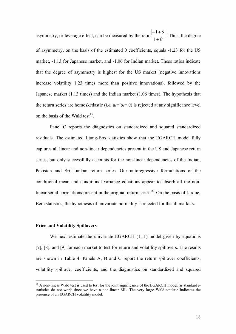
17
asymmetry, or leverage effect, can be measured by the ratioθθ
++−
11
. Thus, the degree
of asymmetry, on the basis of the estimated θ coefficients, equals -1.23 for the US
market, -1.13 for Japanese market, and -1.06 for Indian market. These ratios indicate
that the degree of asymmetry is highest for the US market (negative innovations
increase volatility 1.23 times more than positive innovations), followed by the
Japanese market (1.13 times) and the Indian market (1.06 times). The hypothesis that
the return series are homoskedastic (i.e. a1= b1= θ) is rejected at any significance level
on the basis of the Wald test15.
Panel C reports the diagnostics on standardized and squared standardized
residuals. The estimated Ljung-Box statistics show that the EGARCH model fully
captures all linear and non-linear dependencies present in the US and Japanese return
series, but only successfully accounts for the non-linear dependencies of the Indian,
Pakistan and Sri Lankan return series. Our autoregressive formulations of the
conditional mean and conditional variance equations appear to absorb all the non-
linear serial correlations present in the original return series16. On the basis of Jarque-
Bera statistics, the hypothesis of univariate normality is rejected for the all markets.
Price and Volatility Spillovers
We next estimate the univariate EGARCH (1, 1) model given by equations
[7], [8], and [9] for each market to test for return and volatility spillovers. The results
are shown in Table 4. Panels A, B and C report the return spillover coefficients,
volatility spillover coefficients, and the diagnostics on standardized and squared
15 A non-linear Wald test is used to test for the joint significance of the EGARCH model, as standard t-statistics do not work since we have a non-linear ML. The very large Wald statistic indicates the presence of an EGARCH volatility model.
18

standardized residuals respectively. The full model considers both return and volatility
spillovers from the world source of shocks (the US) and the regional source of shocks
(Japan) to the three small emerging markets. In terms of first moment
interdependencies (return spillovers), there are positive significant return spillovers
from the US to India, Pakistan, and Sri Lanka respectively; all three US return
spillover coefficients (0.0989, 0.0382, and 0.0269) are statistically significant at
conventional levels. There is a positive significant return spillover from Japan to
Pakistan, but there are negative significant return spillovers from Japan to India and
Sri Lanka. Again, all three Japanese return spillover coefficients (-0.0346, 0.0600, and
-0.0376) are statistically significant. Moreover, the magnitude of the spillover
coefficients varies from a low of 0.0269 from the US to Sri Lanka to a high of 0.0989,
from the US to India.
TABLE 4 ABOUT HERE
Turning to second moment interdependencies (volatility spillovers), a
statistically significant spillover effect exists from US to India at the 10 per cent level
of significance, from US to Sri Lanka at the 1 per cent level, and from Japan to
Pakistan at the 5 per cent level. The magnitude of the volatility spillover coefficients
also varies. Specifically, the coefficient from the US to Sri Lanka (0.0209) is greater
than its counterparts from Japan to Pakistan (0.0097), and from the US to India
(0.0056); these findings indicate that the US, proxying for the world factor as a source
of shocks, has more impact on the Asian small markets. In addition, the coefficient
measuring asymmetry, θ, is significant for the Indian and Sir Lankan markets, which
16 Higher-order lags could not eliminate the linear serial correlation present in the Indian, Pakistan and
19

means that any negative news (innovations) from the US market increase volatility
more than positive news of similar size from the same market. Thus, both the Indian
and Sri Lankan markets present evidence consistent with an asymmetric response of
volatility to innovations from the US market. Numerically, bad news from the US
market for Indian and Sri Lankan markets have 1.06 times, and 1.07 times the impact
of good news as indicated by the relative asymmetry ratio. The spillovers are
symmetric for the Pakistan market since the coefficient measuring asymmetry is
insignificant.
Comparing the coefficients from the univariate EGARCH model (restricted
model) with those of the spillover model (unrestricted model) (i.e. Tables 3 and 4,
respectively), we can see that both sets of results are consistent. The coefficients α1, α2
(for the one-lag and two-lag conditional means) and b1 (for the one-lag conditional
variances) all are highly significant; b1 is close to unity as well. These findings clearly
indicate that both the returns and volatility of all three small markets respond to their
own past information. Thus, current information for a market remains important for
all future forecasts of the conditional mean and conditional variance of that market.
Conditional volatilities of the returns in the Pakistan and Sri Lankan markets
respond symmetrically to their own past innovations; the θ coefficients reported in
Table 3 for these two markets are insignificant. Also, evidence of asymmetric
volatility transmission from either of the developed markets to the Pakistan market is
not present; the θ coefficient reported in Table 4 for this market is insignificant.
However, after taking into account volatility spillover, the Sri Lankan market
becomes sensitive to news originating from the US market more strongly when the
news is ‘bad’ than when the news is ‘good’. The Indian market also responds
Sri Lankan return series.
20
asymmetrically to its own past innovations and also to world shocks; both the θ
coefficients reported in Tables 3 and 4 are negative and significant. We use the
likelihood ratio (LR) statistic to test the hypothesis that return and volatility spillovers
from the two developed markets to three small markets are jointly zero (i.e. the
univariate EGARCH model versus the spillover model). The null hypothesis cannot
be rejected at any significance level, implying the importance of return and volatility
spillovers. The Ljung-Box statistics for the standardized and squared standardized
residuals reported in this unrestricted model indicate the presence of limited spillover
effects as the values reported in the table are very close to those calculated for the
restricted model. The Jarque-Bera normality test statistics indicate that standardized
residuals for all three indices exhibit strong deviations from normality. In short, the
existence of first and second moment interdependencies points to the presence of a
global marketplace; however, the degree of interdependencies is limited.
Subperiod Price and Volatility Spillovers
The Asian financial crisis started in mid-1997 and lasted until the end of 1999.
The most directly affected nations were from Southeast Asia, namely Malaysia,
Thailand, the Philippines and Indonesia. However, other countries soon became
affected. Due to “financial contagion”, markets fell across the globe and the
implications of the Asian financial turmoil became far-reaching. For example, in the
US the Dow Jones Industrial Average fell by 554 points on October 27, 1997. The
crisis badly affected Japan which was the biggest trading partner of the main Asian
countries affected and the main supplier of foreign capital to Asian markets.
TABLE 5 ABOUT HERE
21
The results for the unrestricted model (i.e. univariate EGARCH(1,1) with
spillover effect) for the three sub-periods are reported in Table 5. Coefficient a1
(measuring ARCH effect) and b1 (measuring volatility persistence) are significant for
almost all markets in the three periods. The α1 coefficient (measuring the return
persistence) is significant on average, except for India during in-crisis period and for
Pakistan during in- and post-crisis periods. The findings are consistent with the results
reported in Table 4 for the entire period; that is, for these small emerging markets,
past information can be used to forecast both stock market returns and variance.
Finally, the Ljung-Box statistics for the standardized and squared standardized
residuals indicate that the univariate EGARCH model with spillover effects are
correctly specified.
For the pre-crisis period, there is evidence of return spillovers from Japan to
all three small markets. There is also evidence of volatility spillovers from Japan to
the Pakistan and Sri Lankan markets. However, these spillovers are symmetric since
the θ coefficients (measuring the asymmetry) for both markets are insignificant. For
the in-crisis period, the Indian market shows evidence of return spillovers from both
the US and Japanese markets; the Pakistan market also shows signs of return
spillovers from the Japanese market. There is no evidence of return spillovers for Sri
Lankan markets and also no evidence of volatility spillovers for any market.
However, the θ coefficient is significant for the Indian and Pakistan markets, implying
both markets respond asymmetrically to their own past innovations. For the post-crisis
period, there is evidence of both return spillovers and volatility spillovers from the US
market to the Indian, Pakistan, and Sri Lankan markets. In addition, there is some
evidence of return spillovers from the Japanese to the Pakistan market and volatility
22
spillovers from the Japanese to the Indian market. However, the volatility spillovers
are only asymmetric in the Indian market as the coefficient θ is only significant for
India. Thus, the Indian market appears to respond asymmetrically to its own past
innovations and to innovations from the two developed markets as well.
A comparison of the results from the three sub-periods reveals that during the
crisis the small markets are comparatively isolated. In more recent years, however,
these markets have grown more interdependent in the sense that information affecting
asset prices has become more global in nature. We also find that during the pre-crisis
period, these small markets are more responsive to price changes in the Japanese
market which suggests that a regional factor dominates the source of spillovers.
However, during the post-crisis period, the small markets have become more sensitive
to news originating in the US market which indicates that the world factor is the
source of spillovers. Even though we find significant volatility spillovers in these
markets, the volatility transmission is not all asymmetric in the sense the bad news (a
market decline) in one market has a greater impact on the volatility of the next market
to trade.
Discussion
Since governments have implemented financial liberalisation policies, the
capital markets in South Asian countries have become more dependent upon news
from their developed market counterparts which are often the sources of capital
outflows. This fact is confirmed by the findings of significant return spillovers from
both the world’s largest (the US) and the region’s largest (the Japanese) stock markets
to all three South Asian stock markets.
23
The return and volatility spillovers observed from the US market to the Indian
market are hardly surprising as the US is India’s biggest foreign trade partner as well
as its largest cumulative investor - both in Foreign Direct Investment (FDI) and
Foreign Portfolio Investment (FPI). According to the International Financial Statistics
Yearbook, for example, the FDI inflows from the US constituted about 16 percent of
the total actual inflow into the economy in 2001. Out of the 538 Foreign Institutional
Investors (FIIs) registered with the BSE, 220 were from the US. An investment of
nearly USD7 billion out of a total of USD13 billion by FIIs in the Indian capital
markets was from the US. This accounts for about 47 percent of the net investments
made by the FIIs since 1993. However, FPI inflows are very volatile. For example, in
1998, FDI inflows from the US were negative. As Granger et al. (1999) highlighted,
foreign investments to emerging markets are extremely volatile and depend on
changing economic conditions. Since independence, Pakistan has had to depend on
foreign assistance in its development efforts. Japan is its largest donor and the biggest
investor. According to the International Financial Statistics Yearbook, the share of
financial flows from Japan to Pakistan amounted to 91.9 percent, 39 percent, and 59
percent of total donations in 1998, 1999, and 2000 respectively. The total cumulative
amount of net disbursement from Japan's Official Development Assistance (ODA) to
Pakistan reached USD4 billion through 1999. As a result, it is not too surprising to
find that the volatility of the Japanese capital market influences the volatility of
Pakistan equity values. Due to the small size of Sri Lankan economy, export-oriented
industries are extremely important. Sri Lanka and the US enjoy cordial trade relations.
Since the proportion of exports to the US as a percentage of total exports has reached
an average of 40 percent during 1993-2001, according to International Trade Statistics
24
Yearbook, we would therefore expect the volatility of the US economy to be
transmitted to the Sri Lankan market.
It is interesting to see that the South Asian stock markets do not show any
volatility spillovers from the US and/or Japan during the in-crisis period. The South
Asian countries that were examined in this study have been relatively insulated from
the 1997 financial crisis. One reason might be that the financial sectors of these
counties might not have been libaralised to the extent that is evident in East Asian
countries. Also, these countries, and in particular their companies, are less exposed to
foreign debt.
V. Conclusion
This study investigates the magnitude and changing nature of the return and
volatility spillovers from the US and Japan to the three small South Asian stock
markets: namely India, Pakistan and Sri Lanka. We use a univariate Exponential
Generalized Autoregressive Conditionally Heteroskedastic (EGARCH) spillover
model to account for asymmetries in the volatility transmission mechanism, i.e. the
possibility that bad news in a given market has a greater impact on the volatility of the
returns of an other market than good news. We also attempt to distinguish world
forces (the US) from regional factors (Japan). The tests cover the period 01/01/1993-
31/12/2003. To examine whether or not there are structural shifts in the international
market dynamics, the tests are also conducted for three sub-periods – pre-crisis, in-
crisis, and post-crisis.
A number of findings emerge from the analysis. First, for the entire period
analysed, both world and regional factors are important in explaining returns and
volatility in the three South Asian countries examined, although the world market
25
influence tends to be greater. We find evidence of significant return spillovers from
the US and Japan to all three small markets. We also document evidence of volatility
spillovers from the US to Sri Lanka and from Japan to Pakistan at the 5 per cent
significance level and from the US to India at the 10 per cent significance level.
Second, the volatility transmission mechanism is asymmetric but only from the US
stock market, i.e. negative innovations in US equity prices increase volatility in the
Indian and Sri Lankan stock markets considerably more than positive innovations.
Third, no volatility spillovers existed during the period of Asian crisis. More
spillovers, and spillovers of greater intensity, were uncovered during the post-crisis
period. In most cases, spillovers during the post-crisis period were not asymmetric.
Finally, the relative importance of the world and regional market factors was
influenced by the Southeast Asian financial crisis. The sub-period analysis revealed
that before the crisis, regional factors were more important than their world factor
counterparts; in other words, the Japanese stock market was the source of price and
volatility spillover for the South Asia region. However, after the crisis, the world
factors dominate the regional factors; that is, the US stock market has had a larger
impact on small South Asian stock markets.
26
References
Akgiray, V., 1989. Conditional Heteroskedasticity in Time Series of Stock Returns:
Evidence and Forecasts. Journal of Business 62, 55--80.
Bae, K.H., Karolyi, G.A., 1994. Good News, Bad News and International Spillovers
of Stock Return Volatility Between Japan and the U.S. Pacific-Basin Finance Journal
2, 405--438.
Baele, L., 2002. Volatility Spillover Effects in European Equity Markets: Evidence
from a Regime Switching Model. Working Paper, Ghent University.
Baillie, R.T., Bollerslev, T., 1990. Intra-Day and Inter-Market Volatility in Foreign
Exchange Rates. Review of Economics Studies 58, 565--585.
Bekaert, G., Harvey, C.R., 1995. Time-Varying World Market Integration. Journal of
Finance 50, 403--444.
Bekaert, G., Hodrick, R.J., 1992. Characterizing Predictable Components in Excess
Retruns on Equity and Foreign Exchange Markets. Journal of Finance 47, 467--509.
Becker, K.G., Finnerty, J.E., Gupta, M., 1990. The International Relation between the
U.S. and Japanese Stock Markets. Journal of Finance 45, 1297--1306.
Black, F., 1976. Studies of Stock Market Volatility Changes. Proceedings of the
American Econometrics 31, 307--327.
Bollerslev, T., Chou, R., Kroner, K., 1992. ARCH Modeling in Finance: A Review of
the Theory and Empirical Evidence. Journal of Econometrics 52, 5--60.
Bollerslev, T., Wooldridge, J., 1992. Qusai-maximum Likelihood Estimation and
Inference in Dynamic Models with Time-Varying Covariances. Econometric Reviews
11, 143--172.
27
Booth, G.G., Hatem, J., Vitranen, I., Yli-Olli, P., 1992. Stochastic Modeling of
Security Returns: Evidence from the Helsinki Stock Exchange. European Journal of
Operational Research 56, 98--106.
Booth, G.G., Martikainen, T., Tse, Y., 1997. Price and Volatility Spillovers in
Scandinavian Stock Markets. Journal of Banking and Finance 21, 811--823.
Braun, P., Nelson, D., Sunier, A., 1992. Good News, Bad News, Volatility and Betas.
Working paper, University of Chicago.
Campbell, J.Y., Hamao, Y., 1989. Predictable Stock Returns in the United States and
Japan: A Study of Long-term Capital Market Integration. Working Paper, National
Bureau of Economic Research.
Campbell, J.Y., Hamao, Y. 1992. Predictable Stock Returns in the United States and
Japan: A Study of Long-term Capital Market Integration. Journal of Finance 47, 43--
69.
Chan-Lau, J.A., Ivaschenko, I., 2002. Asian Flu or Wall Street Virus? Price and
Volatility Spillovers of the Tech and Non-Tech Sectors in the United States and Asia.
IMF Working Paper.
Chueng, Y.W., Ng, L.K., 1992. Stock Price Dynamics and Firm Size: An Empirical
Investigation. Journal of Finance 47, 1985--1997.
Cheung, Y.W., Fung, H.G., 1997. Information Flows between Eurodollar Spot and
Futures Markets. Multinational Finance Journal 1, 255--271.
Chin, K., Chan, K.C., Karolyi, A., 1991. Intra day Volatility in the Stock Index and
Stock Index Futures Markets. Review of Financial Studies 4, 657--684.
Christie, A.A., 1982. The Stochastic Behavior of Common Stock Variances: Value,
Leverages and Interest Rate Effects. Journal of Financial Economics 10, 407--432.
28
Engle, R.F., 1982. Autoregressive Conditional Heteroscedasticity with Estimates of
the Variance of United Kingdom Inflation. Econometrica 50, 987—1008.
Engle, R.F., 1990. Discussion: Stock Volatility and the Crash of 87. Review of
Financial Studies 3, 103--106.
Engle, R.F., Ito, T., Lin, W., 1991. Meteor Shower or Heat Waves? Heteroscedastic
Intra-Daily Volatility in the Foreign Exchange Market. Econometrica 58, 525--542.
Engle, R.F., Ng, V., 1993. Measuring and Testing the Impact of News on Volatility.
Journal of Finance 48, 1749--1777.
Eun, C., Shim, S., 1989. International Transmission of Stock Market Movements.
Journal of Financial and Quantitative Analysis 24, 241--256.
Fratzscher, M., 2002. Financial Market Integration in Europe: on the Effects of EMU
on Stock Markets. International Journal of Finance and Economics 7, 165--193.
French, K.R., Schwert, G.W., Stambaugh, R.F., 1987. Expected Stock Returns and
Volatility. Journal of Financial Economics 19, 3--29.
Glosten, L., Jagannathan, R., Runkle, D., 1993. Seasonal Patterns in the Volatility of
Stock Index Excess Returns. Journal of Finance 48, 1779--1801.
Granger, C.W. J., Huang, B.N., Yang, C.W., 1999. A Bivariate Causality Between
Stock Prices and Exchange Rates: Evidence from Recent Asian Flu. University of
California at San Diego (UCSD) Economics Discussion Paper.
Hamao, Y., Masulis, R. Ng, V., 1990. Correlations in Price Changes and Volatility
Across International Stock Markets. Review of Financial Studies 3, 281--307.
Hamilton, J.D., 1994. Time Series Analysis. Princeton University Press, Princeton,
New Jersey.
Harvey, C.R., 1995. Predictable Risk and Returns in Emerging Markets. Review of
Financial Studies. 8, 773--816.
29
Hilliard, J., 1979. The Relationship between Equity Indices on World Exchanges.
Journal of Finance 34, 103--114.
Hsieh, D., 1989. Modeling Heteroskedasticity in Daily Foreign Exchange Rates.
Journal of Business and Economics Statistics 7, 5--33.
Joen, B.N., von Furstenberg, G.M., 1990. Growing International Co-movement in
Stock Price Indexes. Quarterly Review of Economics and Business 30, 15--30.
Kanas, A., 1998. Volatility Spillovers Across Equity Markets: European Evidence.
Applied Financial Economics 8, 245--256.
Karolyi, G.A., 1995. A Multivariate GARCH model of International Transmissions of
Stock Returns and Volatility: the Case of the United States and Canada. Journal of
Business and Economics Statistics 13, 11--25.
Karolyi, G.A., Stulz, R.M., 1996. Why do Markets Move Together? An Investigation
of US-Japan Stock Return Comovements Using ADRs. Journal of Finance 51, 951--
986.
Koch, P.D., Koch, T.W., 1991. Evaluation in Dynamic Linkages across Daily
National Stock Indexes. Journal of International Money and Finance 10, 231--251.
Koutmos, G., 1992. Asymmetric Volatility and Risk Return Tradeoff in Foreign Stock
Markets. Journal of Multinational Financial Management 2, 27--43.
Koutmos, G., Booth, G.G., 1995. Asymmetric Volatility Transmission in International
Stock Markets. Journal of International Money and Finance 14, 747--762.
Lo, A.W., MacKinley, A.C., 1988. Stock Market Prices do not Follow Random
Walks. Review of Financial Studies 1, 41--66.
Ng, A., 2000. Volatility Spillover Effects from Japan and the US to the Pacific-Basin.
Journal of International Money and Finance 19, 207--233.
30
Nelson, D.B., 1991. Conditional Heteroskedasticity in Asset Returns: A New
Approach. Econometrica 59, 347--370.
Pagan, A., Schwert, W., 1990. Alternative Models for Conditional Stock Volatility.
Journal of Econometrics 52, 245--266.
Poon, S.H., Taylor, S.J., 1992. Stock Returns and Volatility: An Empirical Study of
the U.K. Stock Market. Journal of Banking and Finance 37--59.
Scheicher, M., 2001. The Comovements of Stock Markets in Hungary, Poland, and
the Czech Republic. International Journal of Finance and Economics 6, 27--39.
Scholes, M., Williams, J.T., 1977. Estimating Betas from Nonsynchronous Data.
Journal of Financial Economics 5, 309--327.
Susmel, R., Engle, R.F., 1994. Hourly Volatility Spillovers between International
Equity Markets. Journal of International Money and Finance 13, 3--25.
Theodossiou, P., Lee, U., 1993. Mean and Volatility Spillovers across Major National
Stock Markets: Further Empirical Evidence. Journal of Financial Research 16, 337--
350.
Worthington, A., Higgs, H., 2004. Transmission of Equity Returns and Volatility in
Asian Developed and Emerging Markets: A Multivariate GARCH analysis.
International Journal of Finance and Economics 9, 71--80.
31
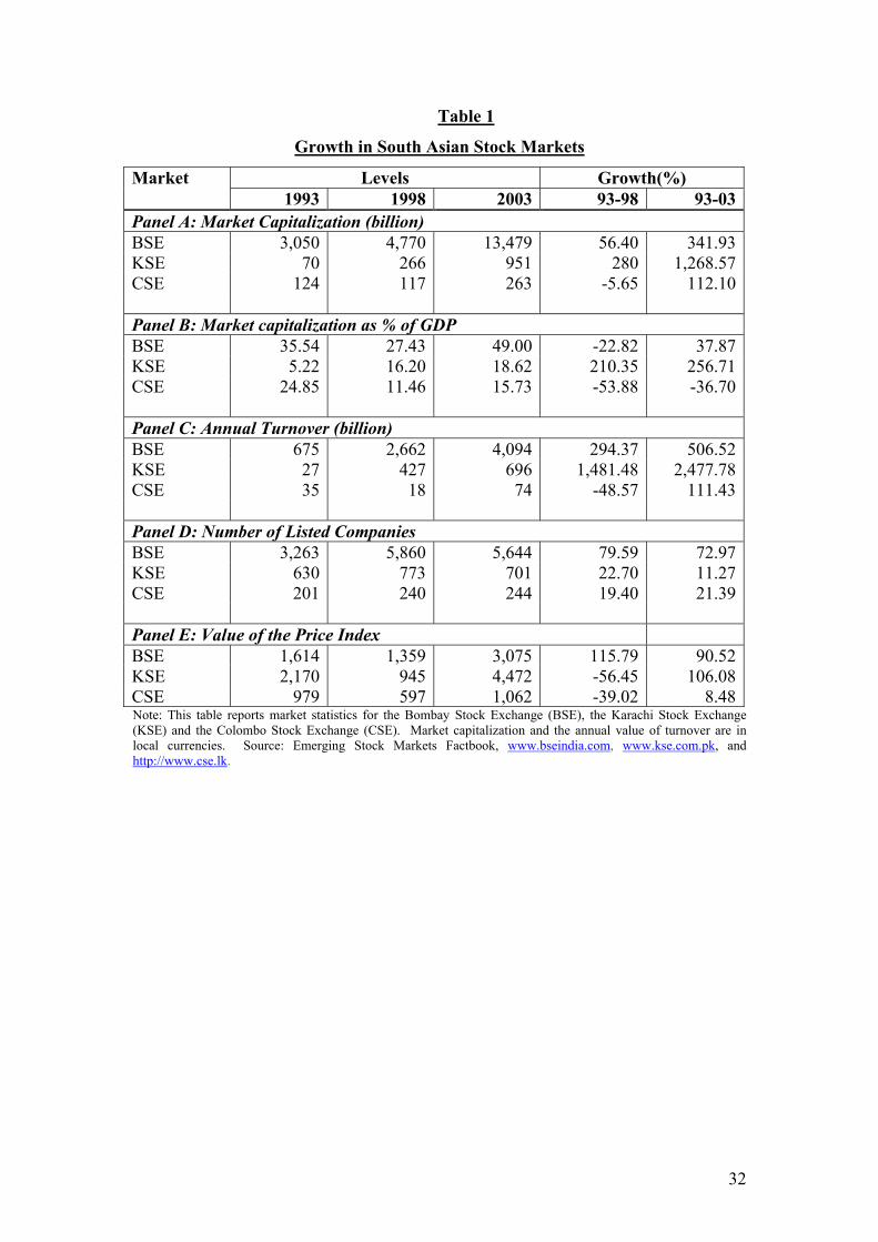
Table 1
Growth in South Asian Stock Markets
Market Levels Growth(%) 1993 1998 2003 93-98 93-03Panel A: Market Capitalization (billion) BSE 3,050 4,770 13,479 56.40 341.93KSE 70 266 951 280 1,268.57CSE 124 117 263 -5.65 112.10 Panel B: Market capitalization as % of GDP BSE 35.54 27.43 49.00 -22.82 37.87KSE 5.22 16.20 18.62 210.35 256.71CSE 24.85 11.46 15.73 -53.88 -36.70 Panel C: Annual Turnover (billion) BSE 675 2,662 4,094 294.37 506.52KSE 27 427 696 1,481.48 2,477.78CSE 35 18 74 -48.57 111.43 Panel D: Number of Listed Companies BSE 3,263 5,860 5,644 79.59 72.97KSE 630 773 701 22.70 11.27CSE 201 240 244 19.40 21.39 Panel E: Value of the Price Index BSE 1,614 1,359 3,075 115.79 90.52KSE 2,170 945 4,472 -56.45 106.08CSE 979 597 1,062 -39.02 8.48Note: This table reports market statistics for the Bombay Stock Exchange (BSE), the Karachi Stock Exchange (KSE) and the Colombo Stock Exchange (CSE). Market capitalization and the annual value of turnover are in local currencies. Source: Emerging Stock Markets Factbook, www.bseindia.com, www.kse.com.pk, and http://www.cse.lk.
32
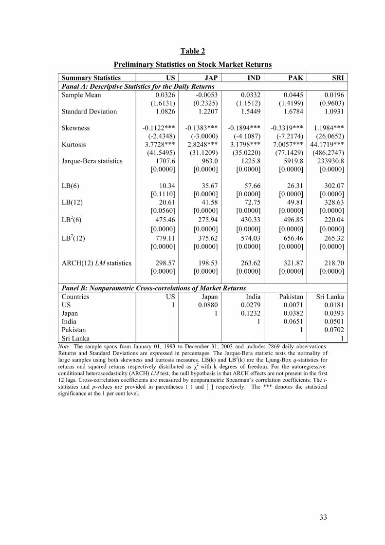
Table 2
Preliminary Statistics on Stock Market Returns
Summary Statistics US JAP IND PAK SRIPanal A: Descriptive Statistics for the Daily Returns Sample Mean 0.0326 -0.0053 0.0332 0.0445 0.0196 (1.6131) (0.2325) (1.1512) (1.4199) (0.9603)Standard Deviation 1.0826 1.2207 1.5449 1.6784 1.0931 Skewness -0.1122*** -0.1383*** -0.1894*** -0.3319*** 1.1984*** (-2.4348) (-3.0000) (-4.1087) (-7.2174) (26.0652)Kurtosis 3.7728*** 2.8248*** 3.1798*** 7.0057*** 44.1719*** (41.5495) (31.1209) (35.0220) (77.1429) (486.2747)Jarque-Bera statistics 1707.6 963.0 1225.8 5919.8 233930.8 [0.0000] [0.0000] [0.0000] [0.0000] [0.0000] LB(6) 10.34 35.67 57.66 26.31 302.07 [0.1110] [0.0000] [0.0000] [0.0000] [0.0000]LB(12) 20.61 41.58 72.75 49.81 328.63 [0.0560] [0.0000] [0.0000] [0.0000] [0.0000]LB2(6) 475.46 275.94 430.33 496.85 220.04 [0.0000] [0.0000] [0.0000] [0.0000] [0.0000]LB2(12) 779.11 375.62 574.03 656.46 265.32 [0.0000] [0.0000] [0.0000] [0.0000] [0.0000] ARCH(12) LM statistics 298.57 198.53 263.62 321.87 218.70 [0.0000] [0.0000] [0.0000] [0.0000] [0.0000] Panel B: Nonparametric Cross-correlations of Market Returns Countries US Japan India Pakistan Sri LankaUS 1 0.0880 0.0279 0.0071 0.0181Japan 1 0.1232 0.0382 0.0393India 1 0.0651 0.0501Pakistan 1 0.0702Sri Lanka 1
Note: The sample spans from January 01, 1993 to December 31, 2003 and includes 2869 daily observations. Returns and Standard Deviations are expressed in percentages. The Jarque-Bera statistic tests the normality of large samples using both skewness and kurtosis measures. LB(k) and LB2(k) are the Ljung-Box q-statistics for returns and squared returns respectively distributed as χ2 with k degrees of freedom. For the autoregressive-conditional heteroscedasticity (ARCH) LM test, the null hypothesis is that ARCH effects are not present in the first 12 lags. Cross-correlation coefficients are measured by nonparametric Spearman’s correlation coefficients. The t-statistics and p-values are provided in parentheses ( ) and [ ] respectively. The *** denotes the statistical significance at the 1 per cent level.
33
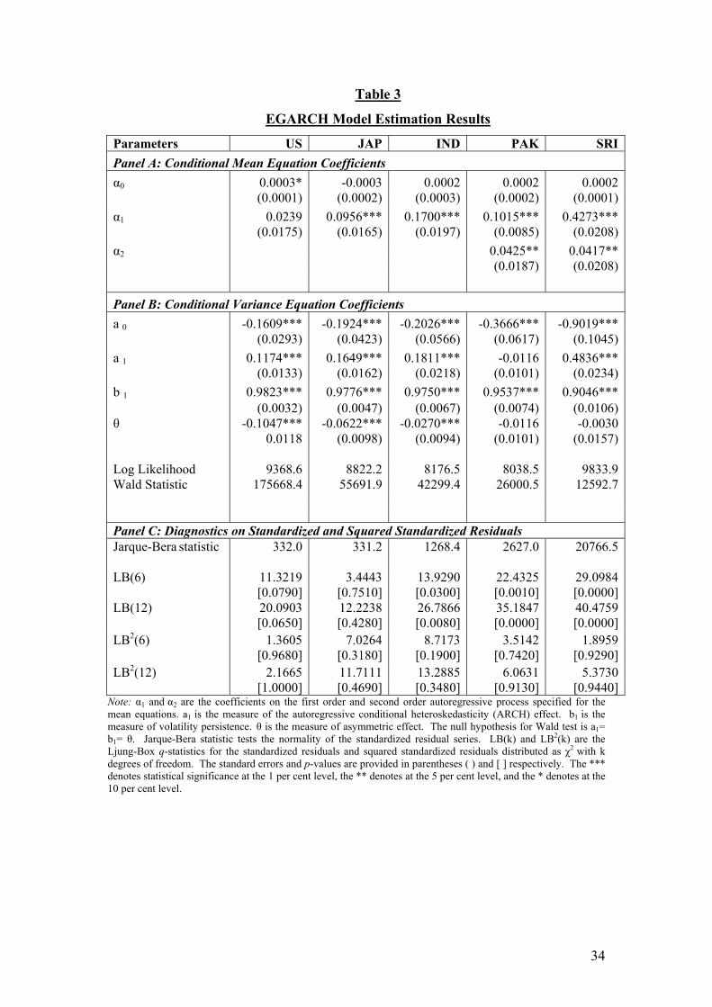
Table 3
EGARCH Model Estimation Results
Parameters US JAP IND PAK SRIPanel A: Conditional Mean Equation Coefficients α0 0.0003* -0.0003 0.0002 0.0002 0.0002 (0.0001) (0.0002) (0.0003) (0.0002) (0.0001)α1 0.0239 0.0956*** 0.1700*** 0.1015*** 0.4273*** (0.0175) (0.0165) (0.0197) (0.0085) (0.0208)α2 0.0425** 0.0417** (0.0187) (0.0208) Panel B: Conditional Variance Equation Coefficients a 0 -0.1609*** -0.1924*** -0.2026*** -0.3666*** -0.9019*** (0.0293) (0.0423) (0.0566) (0.0617) (0.1045)a 1 0.1174*** 0.1649*** 0.1811*** -0.0116 0.4836*** (0.0133) (0.0162) (0.0218) (0.0101) (0.0234)b 1 0.9823*** 0.9776*** 0.9750*** 0.9537*** 0.9046*** (0.0032) (0.0047) (0.0067) (0.0074) (0.0106)θ -0.1047*** -0.0622*** -0.0270*** -0.0116 -0.0030 0.0118 (0.0098) (0.0094) (0.0101) (0.0157) Log Likelihood 9368.6 8822.2 8176.5 8038.5 9833.9Wald Statistic 175668.4 55691.9 42299.4 26000.5 12592.7 Panel C: Diagnostics on Standardized and Squared Standardized Residuals Jarque-Bera statistic 332.0 331.2 1268.4 2627.0 20766.5 LB(6) 11.3219 3.4443 13.9290 22.4325 29.0984 [0.0790] [0.7510] [0.0300] [0.0010] [0.0000]LB(12) 20.0903 12.2238 26.7866 35.1847 40.4759 [0.0650] [0.4280] [0.0080] [0.0000] [0.0000]LB2(6) 1.3605 7.0264 8.7173 3.5142 1.8959 [0.9680] [0.3180] [0.1900] [0.7420] [0.9290]LB2(12) 2.1665 11.7111 13.2885 6.0631 5.3730 [1.0000] [0.4690] [0.3480] [0.9130] [0.9440]
Note: α1 and α2 are the coefficients on the first order and second order autoregressive process specified for the mean equations. a1 is the measure of the autoregressive conditional heteroskedasticity (ARCH) effect. b1 is the measure of volatility persistence. θ is the measure of asymmetric effect. The null hypothesis for Wald test is a1= b1= θ. Jarque-Bera statistic tests the normality of the standardized residual series. LB(k) and LB2(k) are the Ljung-Box q-statistics for the standardized residuals and squared standardized residuals distributed as χ2 with k degrees of freedom. The standard errors and p-values are provided in parentheses ( ) and [ ] respectively. The *** denotes statistical significance at the 1 per cent level, the ** denotes at the 5 per cent level, and the * denotes at the 10 per cent level.
34
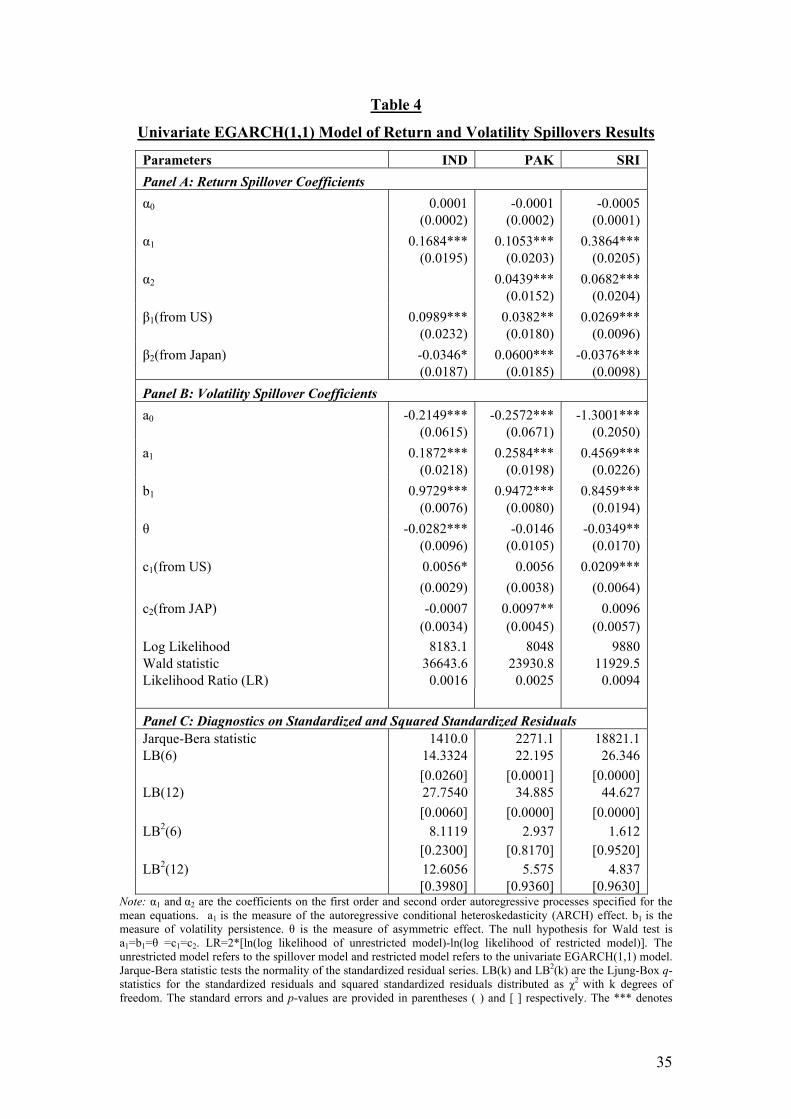
Table 4
Univariate EGARCH(1,1) Model of Return and Volatility Spillovers Results
Parameters IND PAK SRI Panel A: Return Spillover Coefficients α0 0.0001 -0.0001 -0.0005 (0.0002) (0.0002) (0.0001) α1 0.1684*** 0.1053*** 0.3864*** (0.0195) (0.0203) (0.0205) α2 0.0439*** 0.0682*** (0.0152) (0.0204) β1(from US) 0.0989*** 0.0382** 0.0269*** (0.0232) (0.0180) (0.0096) β2(from Japan) -0.0346* 0.0600*** -0.0376*** (0.0187) (0.0185) (0.0098) Panel B: Volatility Spillover Coefficients a0 -0.2149*** -0.2572*** -1.3001*** (0.0615) (0.0671) (0.2050) a1 0.1872*** 0.2584*** 0.4569*** (0.0218) (0.0198) (0.0226) b1 0.9729*** 0.9472*** 0.8459*** (0.0076) (0.0080) (0.0194) θ -0.0282*** -0.0146 -0.0349** (0.0096) (0.0105) (0.0170) c1(from US) 0.0056* 0.0056 0.0209*** (0.0029) (0.0038) (0.0064) c2(from JAP) -0.0007 0.0097** 0.0096 (0.0034) (0.0045) (0.0057) Log Likelihood 8183.1 8048 9880 Wald statistic 36643.6 23930.8 11929.5 Likelihood Ratio (LR) 0.0016 0.0025 0.0094 Panel C: Diagnostics on Standardized and Squared Standardized Residuals Jarque-Bera statistic 1410.0 2271.1 18821.1 LB(6) 14.3324 22.195 26.346 [0.0260] [0.0001] [0.0000] LB(12) 27.7540 34.885 44.627 [0.0060] [0.0000] [0.0000] LB2(6) 8.1119 2.937 1.612 [0.2300] [0.8170] [0.9520] LB2(12) 12.6056 5.575 4.837 [0.3980] [0.9360] [0.9630]
Note: α1 and α2 are the coefficients on the first order and second order autoregressive processes specified for the mean equations. a1 is the measure of the autoregressive conditional heteroskedasticity (ARCH) effect. b1 is the measure of volatility persistence. θ is the measure of asymmetric effect. The null hypothesis for Wald test is a1=b1=θ =c1=c2. LR=2*[ln(log likelihood of unrestricted model)-ln(log likelihood of restricted model)]. The unrestricted model refers to the spillover model and restricted model refers to the univariate EGARCH(1,1) model. Jarque-Bera statistic tests the normality of the standardized residual series. LB(k) and LB2(k) are the Ljung-Box q-statistics for the standardized residuals and squared standardized residuals distributed as χ2 with k degrees of freedom. The standard errors and p-values are provided in parentheses ( ) and [ ] respectively. The *** denotes
35

36
statistical significance at the 1 per cent level, the ** denotes at the 5 per cent level, and the * denotes at the 10 per cent level.
Table 5
Subperiod Return and Volatility Spillovers Results
Pre-Crisis(1172 Observations) In-Crisis(654 Observations) Post-Crisis(1043 Observations) Parameters IND PAK SRI IND PAK SRI IND PAK SRI Panel A: Return Spillover Coefficients α0 -0.0002 -0.0004 -0.0001 0.0005 -0.0003 0.0002 0.0002 0.0009** 0.0001 (0.0005) (0.0003) (0.0001) (0.0006) (0.0007) (0.0003) (0.0004) (0.0004) (0.0002) α1 0.2817*** 0.2227*** 0.5988*** 0.0572 0.0632 0.3804*** 0.1096*** 0.0011 0.3973*** (0.0282) (0.0332) (0.0277) (0.0389) (0.0446) (0.0393) (0.0344) (0.0349) (0.0343) α2 0.0394 0.0066 (0.0334) (0.0351) β1 (from US) -0.0005 0.0451 0.0292 0.1941*** 0.1095 0.0352 0.1280*** 0.0517* 0.0371*** (0.0384) (0.0475) (0.0201) (0.0531) (0.0698) (0.0258) (0.0294) (0.0274) (0.0140) β2 (from Japan) 0.0770** 0.0577* -0.0219* -0.1064** 0.1175* -0.0103 -0.0346 0.0368* -0.0235 (0.0387) (0.0342) (0.0127) (0.0494) (0.0648) (0.0163) (0.0284) (0.0190) (0.0147) Panel B: Volatility Spillover Coefficients a 0 -0.1633* -0.9776*** -1.0115*** -0.9785 -0.2762 -1.2784 -0.6184 -1.1255 -0.8053 (0.0917) (0.3355) (0.2657) 0.4558 0.1616 0.4107 0.1822 0.2765 0.2061 a 1 0.1705*** 0.3137*** 0.5600*** 0.0913 0.2003*** 0.4254*** 0.3496*** 0.3410*** 0.5784*** (0.0282) (0.0428) (0.0482) (0.0592) (0.0354) (0.0683) (0.0567) (0.0446) (0.0412) b 1 0.9762*** 0.8645*** 0.8784*** 0.8858*** 0.9352*** 0.8544*** 0.9266*** 0.8882*** 0.9127*** (0.0093) (0.0358) (0.0191) (0.0560) (0.0205) (0.0412) (0.0224) (0.0243) (0.0146) θ 0.0063 0.0299 0.0463 -0.0893*** -0.0569*** -0.0092 -0.0913*** -0.0329 -0.0467 (0.0143) (0.0243) (0.0304) (0.0293) (0.0241) (0.0359) (0.0248) (0.0248) (0.0320) c1 (from US) 0.0068 -0.0106 -0.0030 -0.0036 0.0173 0.0152 -0.0222*** -0.0235** -0.0232* (0.0056) (0.0095) (0.0113) (0.0108) (0.0109) (0.0164) (0.0095) (0.0105) (0.0122) c2 (from Japan) -0.0039 0.0301*** 0.0208** 0.0012 0.0163 -0.0194 0.0222** 0.0032 0.0073 (0.0050) (0.0090) (0.0098) (0.0160) (0.0127) (0.0168) (0.0103) (0.0100) (0.0109) Log Likelihood 3557.1 3585.0 4362.9 1754.8 1601.9 2278.7 2941.1 2918.5 3356.7 Wald statistic 18907.7 1291.3 3415.6 392.3 3494.8 1052.9 4538.4 2777.6 5517.5 Panel C: Diagnostics on Standardized and Squared Standardized Residuals Jarque-Bera statistic 725.0 180.9 632.4 126.7 550.9 78.8 53.4 461.4 16460.7 LB(6) 6.2091 14.2920 9.3241 9.1736 7.8576 12.1215 8.3227 7.5840 6.0126 [0.4000] [0.0270] [0.1560] [0.1640] [0.2490] [0.0590] [0.2150] [0.2700] [0.4220] LB(12) 13.8916 18.6630 18.2663 17.1463 16.4519 19.5879 15.1638 22.0721 15.3297 [0.3080] [0.0970] [0.1080] [0.1440] [0.1710] [0.0750] [0.2330] [0.0370] [0.2240] LB2(6) 8.2867 5.1431 1.9895 2.6644 1.9672 2.7444 2.7100 7.2896 0.8446 [0.2180] [0.5260] [0.9210] [0.8500] [0.9230] [0.8400] [0.8440] [0.2950] [0.9910] LB2(12) 10.7286 6.4961 4.5923 4.6227 3.9156 38.3501 9.5785 9.6050 2.2708 [0.5520] [0.8890] [0.9700] [0.9690] [0.9850] [0.0000] [0.5910] [0.6510] [0.9990]
Note: α1 and α2 are the coefficients on the first order and second order autoregressive process specified for the mean equations. a1 is the measure of the autoregressive conditional heteroskedasticity (ARCH) effect. b1 is the measure of volatility persistence. θ is the measure of asymmetric effect. The null hypothesis for Wald test is a1=b1=θ =c1=c2. Jarque-Bera statistic tests the normality of the standardized residual series. LB(k) and LB2(k) are the Ljung-Box q-statistics for the standardized residuals and squared standardized residuals distributed as χ2 with k degrees of freedom. The standard errors and p-values are provided in parentheses ( ) and [ ] respectively. The *** denotes statistical significance at the 1 per cent level, the ** denotes at the 5 per cent level, and the * denotes at the 10 per cent level.