return predictability in the treasury market: real rates, inflation, and liquidity
TRANSCRIPT

7/29/2019 Return Predictability in the Treasury Market: Real Rates, Inflation, and Liquidity
http://slidepdf.com/reader/full/return-predictability-in-the-treasury-market-real-rates-inflation-and-liquidity 1/91
Copyright © 2010, 2011, 2013 by Carolin E. Pflueger and Luis M. Viceira
Working papers are in draft form. This working paper is distributed for purposes of comment anddiscussion only. It may not be reproduced without permission of the copyright holder. Copies of workingpapers are available from the author.
Return Predictability in theTreasury Market: Real Rates,
Inflation, and LiquidityCarolin E. PfluegerLuis M. Viceira
Working Paper
11-094
April 25, 2013

7/29/2019 Return Predictability in the Treasury Market: Real Rates, Inflation, and Liquidity
http://slidepdf.com/reader/full/return-predictability-in-the-treasury-market-real-rates-inflation-and-liquidity 2/91
Return Predictability in the Treasury Market:Real Rates, Inflation, and Liquidity
Carolin E. Pflueger and Luis M. Viceira1
First draft: July 2010This version: April 2013
Abstract
This paper decomposes excess return predictability in U.S. and U.K. inflation-indexed andnominal government bonds. We find that nominal bonds reflect time-varying inflation andreal rate risk premia, while inflation-indexed bonds reflect time-varying real rate and liquidityrisk premia. These three risk premia exhibit quantitatively similar degrees of time variation.We estimate a systematic liquidity premium in U.S. inflation-indexed yields over nominalyields, which declined from 100 bps in 1999 to 30 bps in 2005 and spiked to over 150 bpsduring the crisis 2008-2009. We find no evidence that shocks to relative inflation-indexedbond issuance generate return predictability.
JEL Classification: G12Keywords: Expectations Hypothesis; Term structure; Real interest rate risk; Inflation risk;Inflation-Indexed Bonds
1Pflueger: University of British Columbia, Vancouver BC V6T 1Z2, Canada. Email [email protected]. Viceira: Harvard Business School, Boston MA 02163 and NBER. Email [email protected]. We thank Tom Powers and Haibo Jiang for excellent research assistance. We are grateful toJohn Campbell, Kent Daniel, Graig Fantuzzi, Michael Fleming, Josh Gottlieb, Robin Greenwood, ArvindKrishnamurthy, George Pennacchi, Michael Pond, Matthew Richardson, Jeremy Stein, to seminar partic-ipants at the NBER Summer Institute 2011, the Econometric Society Winter Meeting 2011, the Federal
Reserve Board, the European Central Bank, the New York Federal Reserve, the Foster School of Business atthe U. of Washington, the HBS-Harvard Economics Finance Lunch and the HBS Finance Research Day forhelpful comments and suggestions. We are also grateful to Martin Duffell and Anna Christie from the U.K.Debt Management Office for their help providing us with U.K. bond data. This material is based upon worksupported by the Harvard Business School Research Funding. This paper was previously circulated underthe title “An Empirical Decomposition of Risk and Liquidity in Nominal and Inflation-Indexed GovernmentBonds”.

7/29/2019 Return Predictability in the Treasury Market: Real Rates, Inflation, and Liquidity
http://slidepdf.com/reader/full/return-predictability-in-the-treasury-market-real-rates-inflation-and-liquidity 3/91
There is wide consensus among financial economists that returns on nominal U.S. Trea-
sury bonds in excess of Treasury bills are predictable at different investment horizons. Pre-
dictor variables include forward rates (Fama and Bliss, 1987), the slope of the yield curve
(Campbell and Shiller, 1991), and a linear combination of forward rates (Cochrane and Pi-
azzesi, 2005). This paper conducts a joint empirical analysis of the sources of excess bond
return predictability in both nominal and inflation-indexed bonds in the U.S. and the U.K.
Importantly, this joint examination helps to distinguish between different explanations that
have been proposed for excess return predictability in nominal bonds.
The question of whether expected excess returns on inflation-indexed bonds are time-
varying is also important on its own. This question remains relatively unexplored, partly
due to the short history of U.S. inflation-indexed bonds (Campbell, Shiller, and Viceira,
2009). Pflueger and Viceira (2011) show preliminary evidence of excess return predictability
in U.S. Treasury Inflation-Protected Securities (or TIPS) but do not identify its sources. We
examine three potential sources of excess return predictability in inflation-indexed bonds:
time-varying real interest rate risk, time-varying liquidity risk, and market segmentation
between inflation-indexed and nominal bond markets.
We find strong evidence that both time-varying real rate risk premia and time-varying
inflation risk premia contribute to return predictability in nominal government bond excess
returns. Inflation risk premia explain as much time variation in predicted nominal bond
excess returns as do real rate risk premia both in the U.S. and the U.K., suggesting that
a complete theory of nominal bond return predictability needs to incorporate both time-
varying nominal and real risks.
Liquidity explains a substantial fraction of the variation in U.S. and U.K. breakeven, or
1

7/29/2019 Return Predictability in the Treasury Market: Real Rates, Inflation, and Liquidity
http://slidepdf.com/reader/full/return-predictability-in-the-treasury-market-real-rates-inflation-and-liquidity 4/91
the spread between nominal and inflation-indexed bond yields of similar maturity. Novel and
unique to our paper is the finding that the liquidity component in breakeven predicts the
return differential between nominal and inflation-indexed bonds due to liquidity. The U.S.
estimated return differential due to liquidity exhibits a highly significantly positive CAPM
beta with respect to the stock market, but its U.K. counterpart does not. This finding
suggests that U.S. TIPS investors bear systematic risk due to time-varying liquidity and
should be compensated in terms of a return premium.
Although there is wide consensus among financial economists that nominal bond excess
returns are predictable, there is no agreement about what drives this predictability. Proposed
theories of nominal bond excess return predictability differ dramatically in the weights on
real and nominal factors and in the sources of real risk premia.
One hypothesis is that excess return predictability results from time variation in the
aggregate price of risk. Campbell and Cochrane (1999) propose a model where the represen-
tative investor exhibits difference habit preferences over aggregate consumption. Their model
generates a time-varying price of risk, and matches the evidence on predictability in aggre-
gate stock returns from the aggregate price-dividend ratio. Building on this work, Wachter
(2006) shows that a model with time-varying real interest rates can generate nominal bond
excess return predictability from the yield spread of the type documented in Campbell and
Shiller (1991).
A second hypothesis is that excess return predictability results from time variation in
expected aggregate consumption growth or its volatility. The long-run consumption risk
model of Bansal and Yaron (2004) and Bansal, Kiku, and Yaron (2010) emphasizes this
possibility. Bansal and Shaliastovich (2012) show that this, combined with time-varying
2

7/29/2019 Return Predictability in the Treasury Market: Real Rates, Inflation, and Liquidity
http://slidepdf.com/reader/full/return-predictability-in-the-treasury-market-real-rates-inflation-and-liquidity 5/91
inflation volatility, can explain nominal Treasury bond predictability.
If excess bond return predictability is entirely due to time-varying habit or long-run
consumption risk, then we should observe excess return predictability in real (or inflation-
indexed) bonds, since real, not nominal, factors drive the predictability of excess nominal
bond returns. Moreover, the excess return on nominal bonds over inflation-indexed bonds
should not be predictable.
A third hypothesis is that the nominal nature of bonds is an important source of time-
varying risk premia. In this case, we should find that the wedge between nominal and
inflation-indexed bond returns is predictable. Time-varying inflation risk drives bond return
predictability in the time-varying rare disasters framework of Gabaix (2012). Bansal and
Shaliastovich (2013) report that without the inflation risk channel the amount of return
predictability in their model is greatly reduced. In the model of Buraschi and Jiltsov (2005),
both time-varying real and nominal risk premia are important sources of bond excess return
predictability. Campbell, Sunderam, and Viceira (2013) propose a model of the term struc-
ture of interest rates in which a time-varying covariance of inflation with the real stochastic
discount factor generates a time-varying systematic inflation risk premium and nominal bond
excess return predictability. Piazzesi and Schneider (2006) model the slope of the nominal
yield curve when inflation is a predictor of consumption growth.
We contribute to this discussion by providing a new set of empirical phenomena, which
a well specified model of bond return predictability should aim to match: substantial pre-
dictability in both real bond excess returns and in the differential between nominal and real
bond excess returns. Moreover, we find that time-varying real rate risk premia and time-
varying inflation risk premia can switch sign. Both types of risk premia can contribute either
3

7/29/2019 Return Predictability in the Treasury Market: Real Rates, Inflation, and Liquidity
http://slidepdf.com/reader/full/return-predictability-in-the-treasury-market-real-rates-inflation-and-liquidity 6/91
positively or negatively to expected nominal bond returns.
This paper differs from nominal term structure models, such as Campbell, Sunderam,
and Viceira (2013), in one key respect: we quantify time variation in inflation and real rate
risk premia without relying on specific modeling restrictions. In contrast, our decomposition
of bond risk premia should be valid for a wide range of nominal term structure models.
This paper also differs from Campbell, Sunderam, and Viceira (2013) in that it finds and
corrects for an economically significant liquidity risk premium, which could otherwise distort
estimates of inflation and real rate risk premia.
Our empirical exercise carefully addresses two potentially confounding reasons of price
divergence between nominal and inflation-indexed bonds. First, market participants and
financial economists have argued that the market for U.S. inflation-indexed bonds is not as
liquid as the market for nominal bonds.2 It is natural to expect that TIPS might have been
less liquid than nominal Treasury bonds in their early years of learning and supply buildup.
In addition, liquidity differentials between the nominal bond market and the inflation-indexed
bond market might persist even as inflation-indexed bond markets mature. For any investor
the riskless asset is an inflation-indexed bond whose cash flows match his consumption
plan (Campbell and Viceira, 2001, Wachter, 2003), so that inflation-indexed bonds should
typically be held by buy-and-hold investors.
This liquidity differential might result in a liquidity discount on inflation-indexed bonds
relative to nominal bonds and a return differential between both types of bonds controlling
2For evidence of relatively lower liquidity in TIPS see D’Amico, Kim, and Wei (2008), Campbell, Shiller,and Viceira (2009), Fleckenstein, Longstaff, and Lustig (2010), Fleming and Krishnan (2009), Dudley,Roush, and Steinberg Ezer (2009), Gurkaynak, Sack, and Wright (2010), Christensen and Gillan (2011),and Haubrich, Pennacchi, and Ritchken (2011).
4

7/29/2019 Return Predictability in the Treasury Market: Real Rates, Inflation, and Liquidity
http://slidepdf.com/reader/full/return-predictability-in-the-treasury-market-real-rates-inflation-and-liquidity 7/91
for all other sources of return. Indeed, over the 11-year period starting in 1999 the average
annualized excess log return on 10 year U.S. TIPS equaled a substantial 4.7%, almost half
a percentage point higher than that on comparable nominal U.S. Treasury bonds. What
portion of this return differential is attributable to differential liquidity? Does the liquidity
differential between both markets move over time? Is there a similar liquidity differential in
the older and more established market for U.K. inflation-indexed bonds?
We estimate the liquidity differential between inflation-indexed and nominal bond yields
using an empirically flexible approach. We regress breakeven onto liquidity proxies while
controlling for proxies of inflation expectations. Liquidity proxies can explain almost as
much variation in U.S. breakeven as can inflation expectation proxies, consistent with similar
results in Gurkaynak, Sack, and Wright (2010) and D’Amico, Kim, and Wei (2010). Liquidity
variables have smaller, but still significant, explanatory power for U.K. breakeven. After
adjusting for liquidity, our findings suggest that U.S. liquidity-adjusted breakeven inflation
has been quite stable and close to three percent over our sample period, while U.K. breakeven
inflation has trended upwards from three to four percent. U.S. liquidity-adjusted breakeven
inflation remained above 1.7% during the financial crisis, while realized breakeven inflation
was close to zero or even negative for some maturities, suggesting that low realized breakeven
inflation may not have reflected investors’ long-term deflationary fears but relative illiquidity
in U.S. TIPS.
We find a statistically significant and economically important time-varying liquidity com-
ponent in U.S. breakeven. Over our sample period the yield on U.S. TIPS has been about
69 basis points larger on average than it would have been if TIPS had been as liquid as
nominal Treasury bonds. This high average reflects extraordinary events associated with
5

7/29/2019 Return Predictability in the Treasury Market: Real Rates, Inflation, and Liquidity
http://slidepdf.com/reader/full/return-predictability-in-the-treasury-market-real-rates-inflation-and-liquidity 8/91
very low liquidity in this market. We find a high liquidity discount in the years following the
introduction of TIPS (about 70 to 100 bps), which we attribute to learning and low trading
volume, and during the fall of 2008 at the height of the financial crisis (beyond 150 bps).
We estimate a much lower but still significant liquidity discount of between 30 to 70 bps
between 2004 and 2007 and after the crisis. The liquidity premium in U.K. inflation-indexed
gilt yields has been lower on average at 50 bps and has steadily declined over time.
A second complication in using inflation-indexed bonds to identify the systematic sources
of bond excess return predictability is the possibility that the inflation-indexed bond market
and the nominal bond market might be segmented. Recent research has emphasized the
role of limited arbitrage and bond investors’ habitat preferences to explain predictability
in nominal bond returns (Modigliani and Sutch, 1966, Vayanos and Vila, 2009). It seems
plausible that the preference of certain investors, such as pension funds with inflation-indexed
liabilities, for real bonds and the preference of others, such as pension funds with nominal
liabilities, for nominal bonds might lead to imperfect market integration between nominal
and inflation-indexed markets.
We investigate this market segmentation hypothesis using the approach of Greenwood and
Vayanos (2008) and Hamilton and Wu (2010). We find no evidence that market segmentation
and bond supply effects explain breakeven or generate predictability in the relative returns
of inflation-indexed and nominal bonds in the U.S. or the U.K. One potential interpretation
for this finding could be that governments adjust issuance according to investor demand for
the different types of securities, effectively acting as arbitrageurs between the two markets.
Conditional on our estimates of liquidity-adjusted returns, we test whether nominal bond
excess return predictability is due to time-varying real interest risk or time-varying infla-
6

7/29/2019 Return Predictability in the Treasury Market: Real Rates, Inflation, and Liquidity
http://slidepdf.com/reader/full/return-predictability-in-the-treasury-market-real-rates-inflation-and-liquidity 9/91
tion risk. Prices of both inflation-indexed and nominal government bonds change with the
economy-wide real interest rate. Consequently, nominal and inflation-indexed bond risk pre-
mia will reflect investors’ perception of real interest rate risk, which may vary over time.
Prices of nominal government bonds, but not inflation-indexed government bonds, also vary
with expected inflation, so inflation risk will impact their risk premia. Adjusting for liquid-
ity differentials, we find that excess returns on nominal bonds over inflation-indexed bonds
are predictable from the term spread in breakeven inflation both in the U.S. and the U.K.
We interpret this empirical finding as evidence that time-varying inflation risk premia are
a source of return predictability in nominal government bonds. We also find that liquidity-
adjusted excess returns on inflation-indexed bonds are predictable from the inflation-indexed
term spread, even though this empirical finding is only marginally statistically significant for
the U.S. We interpret this second finding as evidence that time-varying real risk contributes
to return predictability in nominal government bond excess returns. Finally, we find that
time-varying liquidity risk contributes statistically and economically significantly to excess
returns on inflation-indexed bond excess returns.
The structure of this paper is as follows. Section I estimates liquidity premia in U.S. and
U.K. inflation-indexed bond yields over nominal bond yields. Section II tests the market
segmentation hypothesis in the U.S. and the U.K. Section III tests for and quantifies time-
varying real interest rate risk premia, inflation risk premia, and liquidity risk premia. Section
IV concludes.
7

7/29/2019 Return Predictability in the Treasury Market: Real Rates, Inflation, and Liquidity
http://slidepdf.com/reader/full/return-predictability-in-the-treasury-market-real-rates-inflation-and-liquidity 10/91
I Bond Data and Definitions
A Bond Notation and Definitions
We denote by y$n,t and yTIPS n,t the log (or continuously compounded) yield with n periods
to maturity for nominal and inflation-indexed bonds, respectively. We use the superscript
TIPS for both U.S. and U.K. inflation-indexed bonds. We define breakeven inflation as the
difference between nominal and inflation-indexed bond yields:
bn,t = y$n,t − yTIPS n,t . (1)
Log excess returns on nominal and inflation-indexed zero-coupon n-period bonds held for
one period before maturity are given by:
xr$n,t+1 = ny$n,t − (n− 1) y$n−1,t+1 − y$1,t, (2)
xrTIPS n,t+1 = nyTIPS
n,t − (n− 1) yTIPS n−1,t+1 − y
TIPS 1,t . (3)
The log excess one-period holding return on breakeven inflation is equal to:
xrbn,t+1 = xr$n,t+1 − xrTIPS n,t+1 . (4)
Note that this is essentially the return on a portfolio long long-term nominal bonds and shortlong-term inflation-indexed bonds. This portfolio will have positive returns when breakeven
inflation declines, and negative returns when it increases.
8

7/29/2019 Return Predictability in the Treasury Market: Real Rates, Inflation, and Liquidity
http://slidepdf.com/reader/full/return-predictability-in-the-treasury-market-real-rates-inflation-and-liquidity 11/91
The yield spread is the difference between a long-term yield and a short-term yield:
s$n,t = y$n,t − y$1,t, (5)
sTIPS n,t = yTIPS
n,t − yTIPS 1,t , (6)
sbn,t = bn,t − b1,t. (7)
Inflation-indexed bonds are commonly quoted in terms of real yields, but since xrTIPS n,t+1
is an excess return over the real short rate it can be interpreted as a real or nominal excess
return. We approximate y$n−1,t+1 and yTIPS n−1,t+1 with y$n,t+1 and yTIPS
n,t+1 .
B Yield Data
For the U.S., we use yields from Gurkaynak, Sack, and Wright (2007) and Gurkaynak, Sack,
and Wright (2010, GSW henceforth). GSW construct constant-maturity zero-coupon off-
the-run yields for nominal bonds starting January 1961 and for TIPS starting January 1999
by fitting smoothed yield curves. We focus on 10-year nominal and real yields, because this
maturity has the longest and most continuous history of TIPS outstanding. We measure U.S.
inflation with the all-urban seasonally adjusted CPI, and the short-term nominal interest rate
with the 3 month T-bill rate from the Fama-Bliss riskless interest rate file from CRSP. Our
sample period for yields is 1999.3-2010.12, while that for quarterly excess returns starts in
1999.6.
The principal of inflation-indexed bonds adjusts automatically with a consumer price
index, which in the U.S. is the Consumer Price Index (CPI-U) and in the U.K. is the
9
7/29/2019 Return Predictability in the Treasury Market: Real Rates, Inflation, and Liquidity
http://slidepdf.com/reader/full/return-predictability-in-the-treasury-market-real-rates-inflation-and-liquidity 12/91
Retail Price Index (RPI). Inflation-indexed bond coupons adjust with inflation and equal
the inflation-adjusted principal on the bond times a fixed coupon rate.3
The nominal principal value of U.S. TIPS is guaranteed to never fall below its original
nominal face value. Consequently, a recently issued TIPS, whose nominal face value is
close to its original nominal face values, has a deflation option built into it that is more
valuable than that in a less recently issued TIPS with the same remaining time to maturity.
Grishchenko, Vanden, and Zhang (2011) study the deflationary expectations reflected in the
pricing of the TIPS deflation floor. During normal times the probability of a severe and
prolonged deflation is negligible so that those bonds trade at identical prices, but Wright
(2009) points out some dramatic price discrepancies between recently issued and seasoned
five-year TIPS during the financial crisis. Appendix Figure A.1 illustrates the GSW 10 year
TIPS yield with yields of 10 year TIPS issued at different reference CPI. The GSW yield is
closest to TIPS yields with low reference CPIs. We conclude that the 10 year GSW TIPS
yield does not reflect a significant deflation option.
We use U.K. constant-maturity zero-coupon yield curves from the Bank of England,
which are estimated with spline-based techniques (Anderson and Sleath, 2001). Nominal
yields are available starting in 1970 and real yields are available starting in 1985. We use
20-year yields because those have the longest history.4 In contrast to the U.S., U.K. inflation-
indexed bonds contain no deflation option. We use the sample period 1999.11-2010.12 for
U.K. yields and 2000.2-2010.12 for U.K. quarterly excess returns because liquidity variables
3There are further details such as in inflation lags in principal updating and tax treatment of the couponsthat slightly complicate the pricing of these bonds. More details on TIPS can be found in Viceira (2001),Roll (2004), Campbell, Shiller, and Viceira (2009) and Gurkaynak, Sack, and Wright (2010). Campbell andShiller (1996) offer a discussion of the taxation of inflation-indexed bonds.
4For some months the 20 year yields are not available and instead we use the longest maturity available.The maturity used for the 20 year yield series drops down to 16.5 years for a short period in 1991.
10

7/29/2019 Return Predictability in the Treasury Market: Real Rates, Inflation, and Liquidity
http://slidepdf.com/reader/full/return-predictability-in-the-treasury-market-real-rates-inflation-and-liquidity 13/91
only become available at the end of 1999. We measure inflation with the non seasonally
adjusted Retail Price Index, which is also used to calculate inflation-indexed bond payouts.
U.K. three month Treasury bill rates are from the Bank of England (IUMAJNB).
Since neither the U.S. nor the U.K. governments issue inflation-indexed bills, we build
a hypothetical short-term real interest rate following Campbell and Shiller (1996) as the
predicted real return on the nominal three month T-bill. Our predictor variables include the
lagged real return on the nominal three month T-bill, the lagged nominal T-bill, and lagged
four quarter inflation. Appendix Figure A.2 shows hypothetical short-term real interest
rates and the corresponding regressions are reported in Appendix Table A.I. For simplicity
we assume a zero liquidity premium on one-quarter real bonds. Appendix Table A.VIII
shows that our results are similar if we replace TIPS returns in excess of the estimated real
interest rate with nominal TIPS returns in excess of the nominal T-bill rate.
Finally, although our yield data is available monthly, we focus on quarterly overlapping
bond returns to reduce the influence of high-frequency noise in observed inflation and short-
term nominal interest rate volatility in our tests.
II Estimating the Liquidity Differential Between Inflation-
Indexed and Nominal Bond Yields
Breakeven inflation, or the yield spread between nominal and inflation-indexed bonds with
identical timing of cash flows, should reflect investors’ inflation expectations plus any com-
pensation for bearing inflation risk, if markets are perfectly liquid. However, if the inflation-
11

7/29/2019 Return Predictability in the Treasury Market: Real Rates, Inflation, and Liquidity
http://slidepdf.com/reader/full/return-predictability-in-the-treasury-market-real-rates-inflation-and-liquidity 14/91
indexed bond market is not as liquid as the nominal bond market, inflation-indexed bond
yields might reflect a liquidity premium relative to nominal bond yields.
We pursue an empirical approach to identify the liquidity differential between inflation-
indexed and nominal bond markets in the U.S. and the U.K. We estimate the liquidity
differential by regressing breakeven inflation on measures of liquidity as in Gurkaynak, Sack,
and Wright (2010), while controlling for inflation expectation proxies. We capture different
notions of liquidity through three different liquidity proxies: the nominal off-the-run spread,
relative transaction volume of inflation-indexed bonds and nominal bonds, and proxies for
the cost of funding a levered investment in inflation-indexed bonds.
Time-varying market-wide desire to hold only the most liquid securities might drive
part of the liquidity differential between nominal and inflation-indexed bonds. In ”flight to
liquidity” episodes some market participants suddenly prefer highly liquid securities rather
than less liquid securities. For the U.S., we measure this desire to hold only the most liquid
securities by the nominal off-the-run spread. The Treasury regularly issues new 10 year
nominal notes and the newest “on-the-run” 10 year note is considered the most liquidly
traded security in the Treasury bond market. After the Treasury issues a new 10-year note,
the prior note goes “off-the-run”. The off-the-run bond typically trades at a discount over
the on-the-run bond – i.e., it trades at a higher yield – despite the fact that it offers almost
identical cash flows (Krishnamurthy, 2002).5 The U.K. Treasury market does not have on-
the-run and off-the-run bonds in a strict sense, since the Treasury typically reopens existing
bonds to issue additional debt. We capture liquidity in the U.K. nominal government bond
5In the search model with partially segmented markets of Vayanos and Wang (2001) short-horizon tradersendogenously concentrate in one asset, making it more liquid. Vayanos (2004) presents a model of financialintermediaries and exogenous transaction costs, where preference for liquidity is time-varying and increasingwith volatility.
12

7/29/2019 Return Predictability in the Treasury Market: Real Rates, Inflation, and Liquidity
http://slidepdf.com/reader/full/return-predictability-in-the-treasury-market-real-rates-inflation-and-liquidity 15/91
market with the difference between a fitted par yield and the yield on the most recently
issued 10 year nominal bond. This measure of the smoothness of the nominal yield curve is
similar to Hu, Pan, and Wang (2012). Hu, Pan, and Wang (2012) show that such a measure
can proxy for market-wide liquidity and the availability of arbitrage capital. Due to its close
relation, we refer to this U.K. measure as the “off-the-run spread” for simplicity.
Liquidity developments specific to inflation-indexed bond markets might also generate
liquidity premia. For instance, when U.S. TIPS were first issued in 1997, investors might
have had to learn about them and the TIPS market might have taken time to get established.
More generally, following Duffie, Garleanu and Pedersen (2005, 2007) and Weill (2007), one
can think of the transaction volume of inflation-indexed bonds as a measure of illiquidity
due to search frictions.6 We proxy for this idea with the transaction volume of inflation-
indexed bonds relative to nominal bonds for the U.S. and the U.K., a measure previously
used by Gurkaynak, Sack, and Wright (2010) for U.S. TIPS. Fleming and Krishnan (2009)
previously found that trading activity is a good measure of cross-sectional TIPS liquidity,
lending credibility to relative transaction volume as a time series liquidity proxy.
Finally, we want to capture the cost of arbitraging between inflation-indexed and nominal
bond markets for levered investors, and more generally the availability of arbitrage capital
and the shadow cost of capital (Garleanu and Pedersen, 2011). In the U.S., levered investors
looking for TIPS exposure can either borrow by putting the TIPS on repo or enter into an
asset-swap, which requires no initial capital. An asset-swap is a derivative contract between
two parties, where one party receives the cash flows on a particular government bond (TIPS
or nominal) and pays LIBOR plus the asset-swap spread (ASW ), which can be positive
6See Duffie, Garleanu, and Pedersen (2005, 2007) and Weill (2007) for models of over-the-counter markets,in which traders need to search for counter parties and incur opportunity or other costs while doing so.
13

7/29/2019 Return Predictability in the Treasury Market: Real Rates, Inflation, and Liquidity
http://slidepdf.com/reader/full/return-predictability-in-the-treasury-market-real-rates-inflation-and-liquidity 16/91
or negative. We use the difference between the asset-swap spreads for TIPS and nominal
Treasuries:
ASW spreadn,t = ASW TIPS n,t −ASW $n,t. (8)
A non-levered investor who perceives TIPS to be under priced relative to nominal Treasuries
can enter a zero price portfolio long one dollar of TIPS and short one dollar of nominal
Treasuries. A levered investor can similarly enter a position long one TIPS asset-swap and
short one nominal Treasury asset-swap. This levered investor pays the relative spread (8),
which is typically positive, for the privilege of not having to put up any initial capital. Since
the levered investor holds a portfolio with a theoretical price of zero, this spread reflects the
current and expected relative financing costs of holding the bond position.
The asset-swap spread is likely related to specialness of nominal Treasuries in the repo
market and the lack of specialness of TIPS, which can vary over time. 7 Differences in
specialness might be the result of variation in the relative liquidity of securities, which make
some securities easier to liquidate and hence more attractive to hold than others.
As a robustness analysis, we consider the spread between synthetic breakeven and cash
breakeven. Synthetic breakeven inflation is the fixed rate in a zero-coupon inflation swap.
Zero-coupon inflation swaps are contracts where one party pays the other cumulative CPI
inflation at the end of maturity in exchange for a pre-determined fixed rate. Entering a
zero-coupon inflation swap does not require any initial capital, similarly to entering a TIPS
asset-swap and going short a nominal Treasury asset-swap. The difference between synthetic
7Holders of certain bonds may be able to borrow at ‘special’ collateralized loan rates below general marketinterest rates (Duffie, 1996, Buraschi and Menini, 2002). In private email conversations Michael Flemingand Neel Krishnan report that for the period Feb. 4, 2004 to the end of 2010 average repo specialness was asfollows. On-the-run coupon securities: 35 bps; off-the-run coupon securities: 6 bps; T-Bills: 13 bps; TIPS:0 bps.
14

7/29/2019 Return Predictability in the Treasury Market: Real Rates, Inflation, and Liquidity
http://slidepdf.com/reader/full/return-predictability-in-the-treasury-market-real-rates-inflation-and-liquidity 17/91
breakeven (or breakeven in the inflation swap market) and cash breakeven is therefore the
flip side of the asset-swap spread (Viceira, 2011). We use the asset-swap spread as our
benchmark variable, since it most closely captures the relative financing cost and specialness
of TIPS over nominal Treasuries.
U.K. asset-swap spread or inflation swap data is not available. We use the LIBOR-general
collateral (GC) repo interest-rate spread, which Garleanu and Pedersen (2011) suggest as
a proxy for arbitrageurs’ shadow cost of capital. In contrast to the asset-swap spread, this
measure cannot capture time-varying margin requirements of inflation-indexed bonds relative
to nominal bonds.
The liquidity differential between inflation-indexed and nominal bond markets can also
give rise to a liquidity risk premium: If the liquidity of inflation-indexed bonds deteriorates
during periods when investors would like to sell, as in “flight to liquidity” episodes, risk averse
investors will demand a liquidity risk premium for holding these bonds (Amihud, Mendelson,
and Pedersen, 2005, Acharya and Pedersen, 2005). While the relative transaction volume
of inflation-indexed bonds likely only captures the current ease of trading and therefore
a liquidity premium, the off-the-run spread, the smoothness of the nominal yield curve,
the asset-swap spread and the LIBOR-GC spread are likely to represent both the level of
liquidity and liquidity risk. Our estimated liquidity premium is therefore likely to represent
a combination of current ease of trading and the risk that liquidity might deteriorate.
In order to isolate the liquidity component in breakeven inflation, we control for inflation-
expectations with survey inflation expectations and variables known to forecast inflation.
15

7/29/2019 Return Predictability in the Treasury Market: Real Rates, Inflation, and Liquidity
http://slidepdf.com/reader/full/return-predictability-in-the-treasury-market-real-rates-inflation-and-liquidity 18/91
A Estimation Strategy
When inflation-indexed bonds are relatively less liquid than nominal bonds, we would ex-
pect inflation-indexed bond prices to decrease and inflation-indexed bond yields to increase
relative to nominal bonds. Let bn,t be breakeven inflation, X t a vector of liquidity proxies,
and πet a vector of inflation expectation proxies. To account for this premium, we estimate:
bn,t = a1 + a2X t + a3πet + εt, (9)
Variables indicating less liquidity in the inflation-indexed bond market, such as the off-
the-run spread, the smoothness of the nominal yield curve, the asset-swap spread, and the
LIBOR-GC spread, should enter negatively in (9). Higher relative transaction volume in the
inflation-indexed bond market should enter positively.
Our liquidity variables are normalized to go to zero in a world of perfect liquidity. When
liquidity is perfect, the off-the-run spread, the smoothness of the nominal yield curve, the
asset-swap spread, and the LIBOR-GC spread should equal zero. U.S. and U.K. relative
transaction volumes are normalized to a maximum of zero. Intuitively, we assume that
the U.S. liquidity premium attributable to low transaction volume was negligible during
2004-2007.
We obtain the liquidity premium in inflation-indexed yields relative to nominal yields as
the negative of the variation in bn,t explained by the liquidity variables:
Ln,t = −a2X t. (10)
16

7/29/2019 Return Predictability in the Treasury Market: Real Rates, Inflation, and Liquidity
http://slidepdf.com/reader/full/return-predictability-in-the-treasury-market-real-rates-inflation-and-liquidity 19/91
a2 is the vector of slope estimates in (9). Thus an increase in Ln,t reflects a reduction in the
liquidity of inflation-indexed bonds relative to nominal bonds.
While our liquidity estimate most likely reflects liquidity fluctuations in both nominal
bonds and in inflation-indexed bonds, we have to make an assumption in computing liquidity-
adjusted inflation-indexed bond yields. We could assume that all of the liquidity premium is
in nominal bonds, in which case we would not need to correct inflation-indexed bond yields.
Alternatively, we could assume that the relative liquidity premium is entirely attributable to
inflation-indexed bond illiquidity. To allow for comparison between these two possibilities,
we calculate inflation-indexed bond yields under the second assumption. We refer to the
following variables as liquidity-adjusted inflation-indexed bond yields and liquidity-adjusted
breakeven:
yTIPS,adjn,t = yTIPS n,t − Ln,t, (11)
badjn,t = bn,t + Ln,t. (12)
B Data on Liquidity and Inflation Expectation Proxies
We obtain the U.S. off-the-run spread by subtracting the on-the-run yield to maturity for
a generic 10 year nominal Treasury bond from Bloomberg (USGG10YR) from the 10 year
GSW off-the-run par yield. The U.K. “off-the-run spread” is the difference between the
fitted 10 year nominal par yield available from the Bank of England (IUMMNPY) and the
generic 10 year nominal U.K. bond yield from Bloomberg.
We calculate U.S. relative transaction volume as logTransTIPS
t /Trans$t
. TransTIPS
t
17

7/29/2019 Return Predictability in the Treasury Market: Real Rates, Inflation, and Liquidity
http://slidepdf.com/reader/full/return-predictability-in-the-treasury-market-real-rates-inflation-and-liquidity 20/91
denotes the average weekly Primary Dealers’ transactions volume over the past month and
Trans$t the corresponding figure for nominal bonds from the New York Federal Reserve FR-
2004 survey. We use the transaction volume for nominal coupon bonds with a long time to
maturity because we aim to capture the differential liquidity of TIPS with respect to 10 year
nominal bonds. Including all maturities or even T-bills would also reflect liquidity of short-
term instruments versus long-term instruments. We smooth relative transaction volume
over the past three months because we think of it as capturing secular learning effects rather
than short-term fluctuations in liquidity.8 We normalize the maximum relative transaction
volume to zero. We construct U.K. transaction volume of inflation-indexed gilts relative to
conventional gilts analogously.9
[FIGURE 1 ABOUT HERE]
We obtain asset-swap spread data from Barclays Live. We only have data on ASW spreadn,t
from January 2004, and set it to its January 2004 value of 28 bps before that date. Weobtain 10 year zero-coupon inflation swap data from Bloomberg (USDSW10Y) from July
2004. The U.K. LIBOR-GC spread is the difference between three month British Pound
LIBOR and three month British Pound GC rates from Bloomberg.
Figures 1A and 1B plot the time series of the U.S. and U.K. liquidity variables. The U.S.
off-the-run spread was high during the late 1990s, declined during 2005-2007, and jumped to
8
In 2001 the Federal Reserve changed the maturity cutoffs for which the transaction volumes are reported.Before 6/28/2001 we use the transaction volume of Treasuries with 6 or more years to maturity while starting6/28/2001 we use the transaction volume of Treasuries with 7 or more years to maturity. The series afterthe break is scaled so that the growth in Trans
$ from 6/21/2001 to 6/28/2001 is equal to the growth intransaction volume of all government coupon securities.
9We are grateful to Martin Duffell from the U.K. Debt Management Office for providing us with turnoverdata.
18

7/29/2019 Return Predictability in the Treasury Market: Real Rates, Inflation, and Liquidity
http://slidepdf.com/reader/full/return-predictability-in-the-treasury-market-real-rates-inflation-and-liquidity 21/91
over 50 bps during the financial crisis. U.S. relative transaction volume rises linearly through
2004, stabilizes, and declines modestly after the financial crisis. This pattern suggests that
the liquidity premium due to the novelty of TIPS should have been modest in the period
since 2004. Interestingly, the U.S. Treasury’s renewed commitment to the TIPS issuance
program (Bitsberger, 2003) and the development of synthetic markets occurred at a similar
time.
Finally, the asset-swap spread ASW spreadn,t varies within a relatively narrow range of 21
basis point to 41 basis points from January 2004 through December 2006, and rises sharply
during the financial crisis, reaching 130 bps in December 2008. That is, before the cri-
sis financing a long position in TIPS was about 30 basis more expensive than financing
one in nominal Treasury bonds, but this cost differential rose dramatically after the Lehman
bankruptcy in September 2008. Campbell, Shiller, and Viceira (2009) argue that the Lehman
bankruptcy significantly affected TIPS liquidity, because Lehman Brothers had been very ac-
tive in the TIPS market. The unwinding of its large TIPS inventory in the weeks following its
bankruptcy, combined with a sudden increase in the cost of financing long positions in TIPS
appears to have induced unexpected downward price pressure in the TIPS market. This led
to a liquidity-induced sharp tightening of breakeven inflation associated with a widening of
the TIPS asset-swap spread. The asset-swap spread ASW spreadn,t and the differential between
synthetic and cash breakeven inflation track very closely, as expected.
Figure 1B shows a steady increase in the U.K. relative transaction volume until 2005 and
flat relative transaction volume thereafter. This increase in relative trading volume might
at first seem surprising, since U.K. inflation-indexed gilts have been issued for significantly
longer than their U.S. counterparts. However, Greenwood and Vayanos (2010) argue that the
19

7/29/2019 Return Predictability in the Treasury Market: Real Rates, Inflation, and Liquidity
http://slidepdf.com/reader/full/return-predictability-in-the-treasury-market-real-rates-inflation-and-liquidity 22/91
U.K. pension reform of 2004, which required pension funds to discount future liabilities at
long-term real rates, increased demand for inflation-indexed gilts and it seems plausible that
the same reform also increased trading volume. Figure 1B also shows that the LIBOR-GC
spread peaked during the financial crisis, similarly to the Asset-Swap-Spread in the U.S.,
consistent with the notion that arbitrageurs’ capital was scarce during the financial crisis.
The U.K. off-the-run spread is significantly smoother than in the U.S. This is unsurprising
given the different market structures. The smoother U.K. off-the-run spread might also
indicate that during flight-to-liquidity episodes investors have a preference for U.S. on-the-
run nominal Treasuries.
We use two variables to proxy for U.S. inflation expectations. First, we use the median
10 year CPI inflation forecast from the Survey of Professional Forecasters (SPF), consistent
with the 10 year maturity of U.S. breakeven.10 Long-term survey inflation expectations are
extremely stable over our sample period. Second, we use the Chicago Fed National Activity
Index (CFNAI) to account for the possibility that short-term inflation expectations enter
into breakeven. The CFNAI provides reliable inflation forecasts over 12 month horizons
(Stock and Watson, 1999). It is based on economic activity measures and should especially
reflect inflation expectation fluctuations related to the aggregate economy.
We proxy for U.K. inflation expectations using the Bank of England Public Attitudes
survey. We use the median response to the question “How much would you expect prices in
the shops generally to change over the next 12 months?”. Unfortunately, this is the longest
forecasting horizon available for our sample.
10SPF survey expectations are available at a quarterly frequency and are released towards the end of the middle month of the quarter. We create a monthly series by using the most recently released inflationforecast.
20

7/29/2019 Return Predictability in the Treasury Market: Real Rates, Inflation, and Liquidity
http://slidepdf.com/reader/full/return-predictability-in-the-treasury-market-real-rates-inflation-and-liquidity 23/91
[TABLE I ABOUT HERE]
Table I shows summary statistics for bond yields, breakeven, excess returns, liquidity, and
inflation expectation proxies. Over our sample period, U.S. average breakeven was 2.24% per
annum (p.a.), average TIPS yields were 2.44% p.a., and average U.S. survey inflation was
2.47% p.a. In contrast, average U.K. breakeven exceeded survey inflation over the similar
period 1999.11-2010.12.
Summary statistics suggest that there may have been a substantial liquidity premium
in U.S. TIPS yields relative to nominal Treasury yields, or a substantial negative inflation
risk premium in nominal yields. If breakeven exclusively reflected investors’ inflation expec-
tations, the negative gap between U.S. breakeven and survey inflation would be surprising.
It would be even more surprising in light of findings that the SPF tends to under predict
inflation when inflation is low (Ang, Bekaert, and Wei, 2007).
Realized log excess returns on U.S. TIPS have averaged 4.66% p.a., exceeding the average
log excess returns on U.S. nominal government bonds by 48 basis points (bps) over our
sample. Average log excess returns on U.K. inflation-indexed bonds have been substantially
smaller at only 2.36% p.a., but have exceeded U.K. nominal log excess returns by 1.80% p.a.
C Estimating Differential Liquidity
Table II estimates the relative liquidity premium in inflation-indexed bonds according to (9).
Panel A presents results for U.S. TIPS, and Panel B for U.K. inflation-linked bonds. We add
21

7/29/2019 Return Predictability in the Treasury Market: Real Rates, Inflation, and Liquidity
http://slidepdf.com/reader/full/return-predictability-in-the-treasury-market-real-rates-inflation-and-liquidity 24/91
liquidity proxies one at a time. In both panels, column (4) presents our benchmark estimate
with all liquidity proxies and inflation expectation controls over our full sample. The last
two columns of each panel present results excluding the financial crisis.
[TABLE II ABOUT HERE]
Table IIA column (1) shows that inflation expectation proxies explain 39% of the vari-
ability in U.S. breakeven. CFNAI is statistically significant with a positive slope, suggesting
that short-run inflation expectations influence investors’ long-run inflation expectations. Ta-
ble I shows that the SPF inflation expectations exhibit very little time variation. Table II
suggests that this variation appears to be unrelated to breakeven inflation, after controlling
for our liquidity proxies and CFNAI.
Panel A shows that liquidity measures explain a significant portion of the variability of
U.S. breakeven inflation. The regression R2 increases with the inclusion of every additional
liquidity variable and reaches 70% in column (5). The off-the-run spread alone increases the
regression R2 regression to 60% from 39% as shown in column (2). Appendix Table A.II
shows that each variable alone also explains significant variation in breakeven inflation.
Table IIA shows coefficients whose signs are consistent with intuition and statistically
significant. Breakeven inflation moves negatively with the off-the-run spread with a large
coefficient, suggesting that TIPS yields reflect a strong market-wide liquidity component.
A one standard deviation move in the off-the-run spread of 11 bps tends to go along with
a decrease in breakeven of 9.5 bps in our benchmark estimation (0.87 × 11 bps). These
magnitudes are substantial relative to average breakeven of 224 bps. This empirical finding
22

7/29/2019 Return Predictability in the Treasury Market: Real Rates, Inflation, and Liquidity
http://slidepdf.com/reader/full/return-predictability-in-the-treasury-market-real-rates-inflation-and-liquidity 25/91
indicates that while during a flight-to-liquidity episode investors rush into nominal on-the-
run U.S. Treasuries, they do not buy U.S. TIPS to the same degree, even though both types
of bonds are fully backed by the same issuer, the U.S. Treasury.
The positive and significant coefficient on relative TIPS trading volume indicates that
the impact of search frictions on inflation-indexed bond prices were exacerbated during the
early period of inflation-indexed bond issuance. As TIPS trading volume relative to nominal
Treasury trading volume increased, TIPS yields fell relative to nominal bond yields. Our
empirical estimates suggest that an increase in relative trading volume from its minimum
in 1999 to its maximum in 2004 was associated with an economically significant decrease in
the TIPS liquidity premium of 48 bps.
When the marginal investor in TIPS is a levered investor, we would expect breakeven to
fall one for one in the asset-swap differential. The estimated slope on the asset-swap spread is
at -0.86 well within one standard deviation of the theoretical value of -1. This result suggests
that the buyers and sellers of asset-swaps may have acted to a large extent as the marginal
buyers and sellers of TIPS. The negative and economically significant coefficient on the
asset-swap spread suggests that disruptions to securities markets and constraints on levered
investors were important in explaining the sharp fall in breakeven during the financial crisis,
since the asset-swap spread differential behaves almost like a dummy variable that spikes
up during the financial crisis. We obtain similar results estimating the regression with the
synthetic minus cash breakeven spread instead of the asset-swap spread.
While bond market liquidity was especially variable during the financial crisis, we also find
a strong relationship between breakeven and liquidity proxies during the pre-crisis period.
Column (6) in Panel A shows that before 2007, proxies for inflation expectations explain
23

7/29/2019 Return Predictability in the Treasury Market: Real Rates, Inflation, and Liquidity
http://slidepdf.com/reader/full/return-predictability-in-the-treasury-market-real-rates-inflation-and-liquidity 26/91
30% of the variability of breakeven inflation. Column (7) shows that adding liquidity proxies
more than doubles the regression R2 to 61% and that the off-the-run spread enters with a
strongly negative and significant coefficient.
Since some of the liquidity variables are persistent, one might be concerned about spu-
riousness. If there is no slope vector so that the regression residuals are stationary, Ordi-
nary Least Squares is quite likely to produce artificially large R2s and t-statistics (Granger
and Newbold, 1974, Phillips, 1986, Hamilton, 1994). Table II shows that the augmented
Dickey-Fuller test rejects the presence of a unit root in regression residuals for all regression
specifications at conventional significance levels. Appendix Table A.III shows that the U.S.
regression results in quarterly changes are very similar to those in levels, further alleviating
concerns.
Our estimation of the liquidity premium might rely on extrapolation outside the range
of historically observed liquidity events. The effect of liquidity proxies on the liquidity dif-
ferential between inflation-indexed and nominal bonds might be nonlinear, especially during
events of extreme liquidity or extreme illiquidity. Appendix Tables A.IV reports additional
results including interaction terms. Appendix Table A.IV also reports regressions with the
U.S. TIPS bid-ask spread as an additional natural liquidity. We find that the bid-ask spread
does not enter, suggesting that the other liquidity proxies already incorporate the time-
varying round-trip cost of buying and selling a TIPS.11
Table IIB shows that U.K. survey inflation, which exhibits much larger time series volatil-
ity than its U.S counterpart, explains 51% of the variability in U.K. breakeven. Adding our
11We are grateful to George Pennachi for making his proprietary data on TIPS bid-ask spreads availableto us.
24

7/29/2019 Return Predictability in the Treasury Market: Real Rates, Inflation, and Liquidity
http://slidepdf.com/reader/full/return-predictability-in-the-treasury-market-real-rates-inflation-and-liquidity 27/91
proxies for liquidity increases the regression R2 to 65%. Liquidity proxies enter with the
predicted signs. Interestingly, columns (5) and (6) in the panel show that prior to the finan-
cial crisis, liquidity variables have even greater explanatory power. In the pre-2007 sample,
survey inflation explains 31% of the variability of breakeven inflation, and including the
liquidity variables more than doubles the R2 to 67%. While in the full sample only rela-
tive transaction volume is individually statistically significant, in the pre-2007 sample our
measure of the smoothness of the nominal yield curve also becomes statistically significant.
Again, the augmented Dickey-Fuller tests reject the presence of a unit root for all regression
specifications in the panel. Overall these results suggest that liquidity factors are important
for understanding the time series variability of breakeven inflation both in the U.S. and the
U.K.
[FIGURES 2A AND 2B ABOUT HERE]
Figures 2A and 2B plot U.S. and U.K. liquidity premia as estimated in the benchmark
regressions in Table II (4), Panels A and B. We obtain liquidity premia according to (10). In-
tuitively, liquidity premia equal the negative of the variation explained by liquidity variables
in Table II.
The estimated U.S. liquidity premium, shown in Figure 2A, has averaged 69 bps with a
standard deviation of 24 bps over our sample. Although this average is high, one must take
into account that it reflects periods of very low liquidity in this market. Figure 2A shows a
high liquidity premium in the early 2000’s (about 70-100 bps), but a much lower liquidity
premium between 2004 and 2007 (35-70 bps). The premium shoots up again beyond 150 bps
25

7/29/2019 Return Predictability in the Treasury Market: Real Rates, Inflation, and Liquidity
http://slidepdf.com/reader/full/return-predictability-in-the-treasury-market-real-rates-inflation-and-liquidity 28/91
during the crisis, and finally comes down to 50 bps after the crisis.
The estimated liquidity time series is consistent with the findings in D’Amico, Kim, and
Wei (2008) but in addition we provide an estimate of the liquidity premium during and
after the financial crisis. In recent work Fleckenstein, Longstaff, and Lustig (2010) show
evidence that inflation swaps, which allow investors to trade on inflation without putting up
any initial capital, appear to be mispriced relative to breakeven inflation in the cash market
for TIPS and nominal Treasury bonds. We account for their average mispricing time series
through the difference between synthetic and cash breakeven in column (5) and through the
closely linked asset swap spread in column (4).
The large liquidity premium in TIPS is puzzling given that bid-ask spreads on TIPS are
small. Haubrich, Pennacchi, and Ritchken (2010) report TIPS bid-ask spreads between 0.5
bps up to 10 bps during the financial crisis. It seems implausible that the liquidity premium
in TIPS yields simply serves to amortize transaction costs of a long-term investor.12 As
previously argued, TIPS should be held by buy-and-hold investors. In a simple model of
liquidity, such as in Amihud, Mendelson and Pedersen (2005), transaction costs of 10 bps
can only justify a 1 bp liquidity premium for 10 year TIPS held by buy-and-hold investors.
A simple calculation shows that the estimated liquidity premium in U.S. TIPS, though
puzzlingly large when compared to bid-ask spreads, gives rise to liquidity returns in line
with those on off-the-run nominal Treasuries. Table I shows that the average U.S. off-the-
run spread over our sample period is 21 bps. However, the on-the-run off-the-run liquidity
differential can be expected to converge in 6 months when the new on-the-run nominal 10
year bond is issued. Thus the average annualized return on the liquidity differential between
12See also Wright (2009).
26

7/29/2019 Return Predictability in the Treasury Market: Real Rates, Inflation, and Liquidity
http://slidepdf.com/reader/full/return-predictability-in-the-treasury-market-real-rates-inflation-and-liquidity 29/91
10 year on-the-run and off-the-run nominal Treasury bonds is 21 × 10× 2 bps = 420 bps. In
contrast, the 10 year U.S. TIPS liquidity premium might take as long as 10 years to converge,
giving an average annualized return on U.S. TIPS liquidity of only 65 bps.
The estimated U.K. liquidity premium has a lower average (50 bps) but a similar standard
deviation (24 bps) compared to U.S. liquidity. Figure 2B shows that the estimated U.K.
liquidity premium was initially similar to the U.S. liquidity premium (around 100 bps) and
stabilized around 40 bps after 2005. It even became negative during the financial crisis,
reflecting extremely high relative transaction volume in U.K. inflation-indexed bonds.
[FIGURE 3 ABOUT HERE]
Figures 3A and 3B show liquidity-adjusted U.S. and U.K. breakeven inflation. Our U.S.
benchmark estimation suggests that liquidity-adjusted U.S. breakeven averaged 2.93% with
a standard deviation of 25 bps over our sample. Liquidity-adjusted U.S. breakeven was
substantially more stable than raw U.S. breakeven. Both raw and liquidity-adjusted U.S.
breakeven fell during the financial crisis but the drop was significantly smaller for liquidity-
adjusted breakeven. Adjusting breakeven for liquidity therefore suggests that while investors’
U.S. long-term inflation expectations fell during the crisis, there was never a period when
investors feared substantial long-term deflation in the U.S.
Figure 3B partly attributes the strong upward trend in U.K. breakeven inflation to liq-
uidity. However, even after adjusting for liquidity U.K. breakeven has trended upwards from
around 3% at the beginning of our sample period to around 4% at the end of 2010. In con-
trast to the U.S., U.K. breakeven does not exhibit a pronounced drop during the financial
27

7/29/2019 Return Predictability in the Treasury Market: Real Rates, Inflation, and Liquidity
http://slidepdf.com/reader/full/return-predictability-in-the-treasury-market-real-rates-inflation-and-liquidity 30/91
crisis. Both raw and liquidity-adjusted U.K. breakeven become substantially more volatile
during 2008-2010, potentially due to increased U.K. inflation uncertainty.
III Testing for Preferred Habitat in U.S. and U.K.
Inflation-Indexed and Nominal Bond Markets
Section II shows that liquidity, understood as market factors not directly related to real
interest rate and inflation fundamentals, explains substantial variation in the yield differential
between inflation-indexed and nominal government bonds in the U.S. and the U.K. However,
before decomposing the fundamental sources of bond return predictability, we still need to
test for one additional potential non-fundamental source of return predictability. This section
tests whether between nominal and inflation-indexed bond markets are segmented due to
preferred habitat preferences.
The preferred habitat hypothesis of Modigliani and Sutch (1966) states that the pref-
erence of certain types of investors for specific bond maturities might result in supply im-
balances and price pressure in the bond market. In recent work Vayanos and Vila (2009)
formalize this hypothesis in a theory where risk-averse arbitrageurs do not fully offset the
price imbalances generated by preferred-habitat investors, leading to excess bond return
predictability. Greenwood and Vayanos (2008) and Hamilton and Wu (2010) find empiri-
cal support for this theory using the relative supply of nominal Treasury bonds at different
maturities as a proxy for supply shocks.
We consider a natural extension of the market segmentation hypothesis. Inflation-indexed
28

7/29/2019 Return Predictability in the Treasury Market: Real Rates, Inflation, and Liquidity
http://slidepdf.com/reader/full/return-predictability-in-the-treasury-market-real-rates-inflation-and-liquidity 31/91
and nominal bond markets might be segmented due to different investor clienteles: Certain
types of investors might have a natural preference for inflation-indexed bonds – for example,
conservative long-term investors or pension funds with inflation-indexed liabilities – while
others might have a natural preference for nominal bonds – for example, pension funds
with nominal liabilities or global investors seeking highly liquid, non-defaultable securities
denominated in a strong currency. If there is limited arbitrage capital keeping both markets
tightly connected, we might observe temporary price divergences unrelated to fundamentals.
For example, breakeven inflation could be larger than implied by market expectations of
inflation and inflation risk premia, if there is strong non-fundamental demand of inflation-
indexed bonds. The Treasury can take advantage of this situation by issuing TIPS. Until it
does so, TIPS bonds will appear overpriced relative to fundamentals and breakeven inflation
will be large relative to fundamentals.13 Prices will correct once the Treasury increases the
supply of TIPS, generating a decline in breakeven and negative returns for TIPS holders.
We test whether segmentation between inflation-indexed and nominal bond markets in-
duces relative price fluctuations and return predictability in an empirical setup similar to
Greenwood and Vayanos (2008). If supply is subject to exogenous shocks while clientele de-
mand is stable over time we would expect increases in the relative supply of inflation-indexed
bonds to be correlated with contemporary decreases in breakeven inflation, as the price of
inflation-indexed bonds falls in response to excess supply. Subsequently we would expect to
see positive returns on inflation-indexed bonds as their prices rebound.
13Greenwood and Vayanos (2010) analyze an episode of this nature in the U.K. The U.K. Pensions Act of 2004 provided pension funds with a strong incentive to buy long-maturity and inflation-linked governmentbonds. Pundits and market participants argued that this led to an overpricing of inflation-indexed bondsbecause the government did not immediately increase the issuance of these bonds to keep up with theregulatory driven excess demand for inflation linkers.
29

7/29/2019 Return Predictability in the Treasury Market: Real Rates, Inflation, and Liquidity
http://slidepdf.com/reader/full/return-predictability-in-the-treasury-market-real-rates-inflation-and-liquidity 32/91
Alternatively, it could be the case that bond demand changes over time, while the govern-
ment tries to accommodate changes in demand. This issuance behavior would be consistent
with a debt management policy that tries to take advantage of interest rate differentials
across both markets. In this case, the relative supply of inflation-indexed bonds might be
unrelated to subsequent returns, and possibly even positively correlated with contempora-
neous breakeven inflation.
Let DTIPS t denote the face value of inflation-indexed bonds outstanding and Dt the
combined face value of nominal and inflation-indexed bonds outstanding at time t for either
the U.S. or the U.K. We define relative supply Supplyt and relative issuance ∆Supplyt:
Supplyt = DTIPS t /Dt, (13)
∆Supplyt =DTIPS
t −DTIPS t−1
/DTIPS
t−1 − (Dt −Dt−1) /Dt−1. (14)
We also construct a measure of unexpected relative issuance εSupplyt .14 In Appendix Table
A.XII we conduct Dickey-Fuller tests to find that in the U.S. we cannot reject a unit root
in Supplyt or in ∆Supplyt. However, the year-over-year change in relative issuance appears
stationary and we construct a supply shock εSupplyt as the residual from an autoregression of
14We measure the relative supply of inflation-indexed bonds in the U.S. as the nominal amount of TIPSoutstanding relative to U.S. government TIPS, notes and bonds outstanding. U.K. relative supply is thetotal amount of inflation-linked gilts relative to the total amount of conventional gilts outstanding. Theeconomic report of the president reports U.S. Treasury securities by kind of obligation and reports T-bills,Treasury notes, Treasury bonds and TIPS. The data can be found in Table 85 until 2000 and in Table 87
afterwards at http://www.gpoaccess.gov/eop/download.html. The face value of TIPS outstanding availablein the data is the original face value at issuance times the inflation incurred since then and therefore itincreases with inflation. The numbers include both privately held Treasury securities and Federal Reserveand intra-governmental holdings as in Greenwood and Vayanos (2008). We are deeply grateful to the U.K.Debt Management Office for providing us with data. Conventional U.K. gilts exclude floating-rate anddouble-dated gilts but include undated gilts. The face value of U.K. index-linked gilts does not includeinflation-uplift and is reported as the original nominal issuance value.
30

7/29/2019 Return Predictability in the Treasury Market: Real Rates, Inflation, and Liquidity
http://slidepdf.com/reader/full/return-predictability-in-the-treasury-market-real-rates-inflation-and-liquidity 33/91
∆Supplyt−∆Supplyt−12 with twelve lags. In the U.K. we can reject stationarity in relative
issuance ∆Supplyt, potentially reflecting the less regular U.K. bond issuance cycle. We
therefore construct the U.K. supply shock εSupplyt as the residual from an autoregression of
∆Supplyt with twelve lags.
[FIGURE 4 ABOUT HERE]
Figure 4A plots the relative supply of U.S. TIPS and U.S. 10 year breakeven inflation.
Starting from less than 2% in 1997 TIPS increased to represent over 14% of the U.S. Treasury
coupon bond portfolio in 2008. Subsequently to the financial crisis the U.S. government
issued substantial amounts of nominal notes and bonds, leading to a drop in the relative
TIPS share to 9% in 2010. U.S. breakeven inflation remained relatively steady with a large
drop in the fall of 2008.
Figure 4B illustrates that the relative share of U.K. linkers has increased from about 9%
in 1985 to 16% in 2010. Over the same time period 20 year U.K. breakeven inflation has
fallen, reaching a low of 2.1% in 1998. The increase in inflation-linked bonds outstanding
accelerated noticeably after the U.K. Pension Reform of 2004.
[TABLE III ABOUT HERE]
Table III tests whether breakeven is related to the relative supply measures Supplyt,
∆Supplyt, and Supplyt . If markets are segmented and subject to exogenous supply shocks we
would expect to find negative slope coefficients onto these measures. Panel A in the table
31

7/29/2019 Return Predictability in the Treasury Market: Real Rates, Inflation, and Liquidity
http://slidepdf.com/reader/full/return-predictability-in-the-treasury-market-real-rates-inflation-and-liquidity 34/91
shows results for the U.S., and Panel B shows results for the U.K. We include controls for
inflation expectations in all regressions.
Table IIIA shows that U.S. relative supply enters with a positive and significant coef-
ficient, but the coefficient becomes insignificant when controlling for liquidity proxies and
a time trend. Neither relative issuance nor relative supply shocks εSupplyt appear related to
breakeven, either individually or when controlling for liquidity variables and a time trend.
Table IIIB shows similar empirical results for the U.K. The U.K. results are consistent
between a significantly longer sample period, and a shorter sample period, for which liquidity
controls are available. Relative supply enters with a positive and significant coefficient, but
this coefficient becomes insignificant as we include a time trend in the regression. The time
trend is highly statistically significant and dramatically increases the regression R2. Again,
relative issuance or supply shocks εSupplyt do not enter significantly.
The positive coefficient onto relative supply for both countries could be consistent with
the U.S. and the U.K. governments reacting to increased demand for inflation-linked bonds
by issuing more inflation-indexed bonds, which is consistent with at least U.K. anecdotal
evidence. Unlike the U.S. Treasury, the U.K. Debt Management Office has an irregular
auction calendar and appears to take into account bond demand when deciding the size and
characteristics of bond issues.
Our results in this section can be reconciled with Fleckenstein, Longstaff, and Lustig
(2010), who argue that the supply of Treasury securities affects the relative mispricing of
inflation-indexed and nominal bonds. We use the theoretically motivated relative supply of
inflation-indexed bonds, while they include both the supply of TIPS and of Treasuries sepa-
32

7/29/2019 Return Predictability in the Treasury Market: Real Rates, Inflation, and Liquidity
http://slidepdf.com/reader/full/return-predictability-in-the-treasury-market-real-rates-inflation-and-liquidity 35/91
rately in their regressions. They find that TIPS become relatively more expensive when the
Treasury issues more TIPS, which seems inconsistent with a market segmentation hypoth-
esis. They interpret their results as evidence that markets with liquid on-the-run securities
allow arbitrageurs to drive prices together.
If markets are segmented in the sense of Greenwood and Vayanos (2008) a positive
shock to the relative supply of inflation-indexed bonds should predict lower excess returns
on nominal bonds over inflation-indexed bonds. Table IV finds no evidence that U.S. or
U.K. supply variables predict bond excess returns. Table IV reports regressions of nominal,
inflation-indexed and breakeven returns as defined in (2), (3) and (4) onto lagged relative
supply. Campbell and Shiller (1996) show that the nominal term spread can predict excess
returns on long-term nominal bonds. Moreover, Pflueger and Viceira (2011) show that TIPS
term spreads and breakeven term spreads are significant predictors of the corresponding
excess returns and therefore we control for these spreads in our regressions. We control
for lagged relative inflation-indexed bonds liquidity to control for potentially time-varying
liquidity risk premia.
[TABLE IV ABOUT HERE]
Table IV shows that even after controlling for supply effects, the nominal term spread
forecasts positively nominal bond excess returns and its slope coefficient is significant in the
U.K. over the longer sample period. The breakeven term spread predicts breakeven excess
returns both in the U.S. and the U.K. The inflation-indexed bond term spread predicts
inflation-indexed bond excess returns in the U.K. over the longer sample and is marginally
significant in the U.S. and the U.K. over the shorter 11 year period. Relative supply shocks
therefore cannot explain why term spreads predict excess returns on inflation-indexed bonds
33

7/29/2019 Return Predictability in the Treasury Market: Real Rates, Inflation, and Liquidity
http://slidepdf.com/reader/full/return-predictability-in-the-treasury-market-real-rates-inflation-and-liquidity 36/91
and on nominal bonds in excess of inflation-indexed bonds.
In summary, there is no evidence of relative supply shocks predicting bond excess returns
in either the U.S. or the U.K. These results do not seem consistent with segmented markets
that are subject to exogenous supply shocks. Instead they might indicate that U.S and U.K.
governments accommodate demand pressures from investors for nominal or inflation-indexed
bonds.
IV Decomposing Time-Varying Bond Risk Premia
As shown in Section II, bond market liquidity proxies can explain substantial variation in the
difference between nominal and inflation-indexed yields. This section provides new empirical
evidence on excess bond return predictability using liquidity-adjusted inflation-indexed bond
returns, liquidity-adjusted breakeven returns, and returns due to changes in bond market
liquidity. In Section III, we found no evidence that relative supply shocks and preferredhabitat with limits to arbitrage generate bond return predictability; we therefore interpret
our predictability results as evidence of time variation in real interest rate risk premia,
inflation risk premia, and liquidity risk premia.15
This section decomposes government bond excess returns into returns due to real interest
rates, changing inflation expectations, and liquidity. We test for predictability in each com-
15Pflueger and Viceira (2011) find that TIPS returns are predicted by the TIPS term spread and thatbreakeven inflation returns are predicted by the breakeven term spread. However, they cannot test whetherreal rate risk premia and inflation risk premia are time-varying because they do not adjust for the substantialliquidity component in breakeven. See also Barr and Campbell (1997) and Evans (2003) for evidence onpredictability in inflation-indexed bond excess returns using a significantly shorter U.K. sample with noliquidity adjustment.
34

7/29/2019 Return Predictability in the Treasury Market: Real Rates, Inflation, and Liquidity
http://slidepdf.com/reader/full/return-predictability-in-the-treasury-market-real-rates-inflation-and-liquidity 37/91
ponent separately: Predictability in liquidity-adjusted real bond excess returns would indi-
cate a time-varying real interest rate risk premium, while predictability in liquidity-adjusted
breakeven returns would indicate a time-varying inflation risk premium. Predictability in the
liquidity component of TIPS returns would indicate a time-varying liquidity risk premium.
We compute liquidity-adjusted inflation-indexed and breakeven excess returns by replac-
ing inflation-indexed bond yields and breakeven with their liquidity-adjusted counterparts
(11) and (12):
xrTIPS −Ln,t+1 = nyTIPS,adjn,t − (n− 1) yTIPS,adjn−1,t+1 − y
TIPS 1,t , (15)
xrb+Ln,t+1 = xr$n,t+1 − xr
TIPS −Ln,t+1 . (16)
The expression (15) relies again on the assumption that the liquidity differential is en-
tirely attributable to inflation-indexed bonds. The return on inflation-indexed bonds due to
illiquidity is given by:
rLn,t+1 = − (n− 1)Ln−1,t+1 + nLn,t. (17)
Table V regresses excess returns (15), (16), and (17) onto one-quarter lags of the liquidity-
adjusted real term spreadyTIPS n,t − Ln,t
− yTIPS
1,t , the liquidity-adjusted breakeven term
spread (bn,t + Ln,t) − b1,t, and the estimated liquidity differential between inflation-indexed
and nominal yields Ln,t. Intuitively, the three right-hand-side variables decompose the nomi-
nal term spread, used by Campbell and Shiller (1991) to predict nominal bond excess returns,
into real term structure, inflation, and liquidity components. Table V reports Newey-West
standard errors with three lags and one-sided bootstrap p-values, which account for the
35

7/29/2019 Return Predictability in the Treasury Market: Real Rates, Inflation, and Liquidity
http://slidepdf.com/reader/full/return-predictability-in-the-treasury-market-real-rates-inflation-and-liquidity 38/91
fact that liquidity is estimated.16 For comparison, Appendix Table A.IX reports results for
non-liquidity adjusted excess returns.
[TABLE V ABOUT HERE]
The first two columns in Panel A show that liquidity-adjusted TIPS excess returns are
not statistically significantly predictable according to bootstrap p-values. Of course, this
finding of no predictability might partly be due to our short U.S. sample, which reduces our
statistical power. Columns (1) and (2) of Panel B provide additional evidence from the cross-
section of international inflation-indexed bonds and show strong evidence for excess return
predictability in the U.K. The U.K. real term spread enters with a positive and significant
coefficient even when controlling for liquidity. The liquidity-adjusted breakeven term spread
and lagged liquidity do not enter significantly in columns (1) or (2) either in the U.S. or the
U.K., as one might expect if those variables are unrelated to real interest rate risk.
Columns (3) and (4) in Tables VA and VB show strong evidence that liquidity-adjusted
breakeven excess returns are predictable. Liquidity-adjusted breakeven term spreads predict
breakeven excess returns with coefficients that are large, statistically significant, and similar
across both countries. This empirical finding indicates that that time-varying inflation risk
premia are a source of predictability in nominal bond excess returns and that the nominal
term spread partly reflects time-varying inflation risk premia.
Remarkably, liquidity does not predict liquidity-adjusted real bond or breakeven excess
returns in the U.S. or the U.K. The estimated liquidity differential does not appear related to
16We use a non-parametric block bootstrap with block length 24 months and 2000 replications. SeeHorowitz (2001) for a survey of bootstrap methods.
36

7/29/2019 Return Predictability in the Treasury Market: Real Rates, Inflation, and Liquidity
http://slidepdf.com/reader/full/return-predictability-in-the-treasury-market-real-rates-inflation-and-liquidity 39/91
fundamental bond cash-flow risk, alleviating concerns that estimated liquidity might capture
time-varying inflation risk premia as a result of our estimation strategy.
The last two columns of Tables VA and VB show that liquidity Ln,t predicts quarterly
liquidity returns rLn,t+1 with large and highly significant coefficients. Both in the U.S. and
the U.K., time-varying and predictable liquidity premia are a source of excess return pre-
dictability inflation-indexed bonds. The effect of the liquidity premium on returns is such
that when liquidity in the inflation-indexed bond market is scarce, inflation-indexed bonds
enjoy a higher expected return relatively to nominal bonds, rewarding investors who are
willing to invest into a temporarily less liquid market.
Table V uses inflation-indexed bond returns in excess of a hypothetical real short rate.
Appendix Table A.VII shows that return predictability regressions are very similar if we
include interaction terms in the liquidity estimation. Appendix Table A.VIII shows that
results hold up for tradeable nominal returns on inflation-indexed bond in excess of the
nominal short rate.
The return predictability regressions in Table V provide empirical evidence of time varia-
tion in three different components of bond risk premia: real interest rate risk premia, inflation
risk premia, and liquidity risk premia. The evidence for time-varying inflation risk premia
and liquidity risk premia is highly statistically significant and consistent across U.S. and
U.K. data.
A Economic Significance of Bond Risk Premia
[TABLE VI ABOUT HERE]
37

7/29/2019 Return Predictability in the Treasury Market: Real Rates, Inflation, and Liquidity
http://slidepdf.com/reader/full/return-predictability-in-the-treasury-market-real-rates-inflation-and-liquidity 40/91
We now evaluate the economic significance of time-varying real rate risk premia, infla-
tion risk premia, and liquidity risk premia. The first column of Table VI reports annualized
average excess log returns on real bonds and breakeven, and average log liquidity returns.
We note that our average return calculations are based on log returns with no variance ad-
justments for Jensen’s inequality. For simplicity we refer to the expected liquidity excess
return as a liquidity risk premium, the expected liquidity-adjusted breakeven return as an
inflation risk premium and expected liquidity-adjusted TIPS returns as a real rate risk pre-
mium. Note that the average excess return on inflation-indexed bonds equals the sum of the
liquidity risk premium plus the real rate risk premium and that the average excess return on
nominal bonds equals the sum of the inflation risk premium plus the real rate risk premium.
Table VIA shows that, at 99 bps, the liquidity risk premium accounts for almost one-
fifth of the average realized total U.S. TIPS excess return over this period (see Table I).
Although the average estimated inflation risk premium is economically significant at 52 bps,
it is substantially smaller than the average real interest rate risk premium over the same
time period. Table VIB shows that at 161 basis points, the average estimated liquidity
risk premium is even more substantial in the U.K. Interestingly, the estimated inflation risk
premium in U.K. nominal bonds is negative at -34 bps, helping to explain low average log
excess returns on nominal U.K. bonds (Table I).17
Column (2) of Table VIA shows that U.S. liquidity-adjusted breakeven excess returns
and liquidity-adjusted TIPS excess returns both have small and negative CAPM betas.18
17Our estimates suggest that the negative inflation risk premium estimated by Campbell, Sunderam andViceira (2013) over our sample period might have been partly due to a relative TIPS liquidity premium.
18We compute CAPM betas using the stock market as the proxy for the wealth portfolio. The U.S. excessstock return is the log quarterly return on the value-weighted CRSP index, rebalanced annually, in excess of the log 3-month interest rate. The U.K. excess stock return is the log quarterly total return on the FTSE inexcess of the log 3-month interest rate. In Appendix Table A.X, we find that raw breakeven returns exhibit
38
7/29/2019 Return Predictability in the Treasury Market: Real Rates, Inflation, and Liquidity
http://slidepdf.com/reader/full/return-predictability-in-the-treasury-market-real-rates-inflation-and-liquidity 41/91
By contrast, the beta on U.S. liquidity returns is positive and significant. The positive
liquidity beta implies that TIPS tend to become illiquid relative to nominal Treasury bonds
– or conversely, nominal bonds become liquid relative to TIPS – during stock market drops.
The strong positive covariation between U.S. estimated liquidity returns and stock returns
suggests that investors should expect to earn a premium on TIPS for bearing systematic
variation in liquidity. Consistent with this notion, Appendix Table A.X shows that the
market alpha of liquidity returns is small and insignificant over our full sample. This table
also shows that during the pre-crisis period, liquidity returns have no market exposure and
substantial alpha, suggesting that positive liquidity returns compensate TIPS holders for
the risk that TIPS become less liquid during dramatic drops in the stock market. Appendix
Table A.XI shows that TIPS liquidity returns are not related to innovations in the Pastor-
Stambaugh factor, which captures stock market liquidity, or to the Fama-French factors.
In contrast, column (2) of Table VIB shows that the U.K. liquidity beta is indistin-
guishable from zero. The CAPM beta of U.K. liquidity-adjusted breakeven returns is large,
negative, and statistically significant, suggesting that inflation expectations and thus nomi-
nal interest rates have been pro-cyclical during our sample period. The combined evidence
of procyclical nominal interest rates and low inflation risk premia is consistent with a view
that nominal Treasuries were safe assets and provided investors with sizable diversification
benefits over our sample in the framework of Campbell, Sunderam, and Viceira (2013).
We find that time-varying real rate risk premia, time-varying inflation risk premia and
time-varying liquidity premia are quantitatively equally important sources of return pre-
dictability. Column (3) of Table VI reports roughly similar standard deviations for estimated
a large and negative CAPM beta.
39

7/29/2019 Return Predictability in the Treasury Market: Real Rates, Inflation, and Liquidity
http://slidepdf.com/reader/full/return-predictability-in-the-treasury-market-real-rates-inflation-and-liquidity 42/91
expected liquidity-adjusted real bond excess returns, liquidity-adjusted breakeven returns,
and liquidity returns. The standard deviations in column (3) are in line with the standard
deviation of predicted nominal excess bond returns estimated from standard Campbell and
Shiller (1991) bond return forecasting regressions (Appendix Table A.IX), suggesting that
estimated components of bond excess returns are as predictable as raw excess returns.
[FIGURE 5 ABOUT HERE]
Figure 5 shows predicted 3-month excess returns, labeled real rate risk premia, inflation
risk premia, and liquidity risk premia. While magnitudes may appear large, Figure 5 shows
predicted 3-month returns in annualized units and not predicted 12-month returns. Figure
5A shows that the U.S. inflation risk premium was small or negative 2000-2006. The inflation
risk premium became positive during the period of high oil prices in 2008 and fell to almost
-5% at the beginning of 2009, just when the U.S. real rate risk premium increased sharply.
The U.S. liquidity risk premium was large in the early 2000s, declined steadily during the
decade, and spiked during the financial crisis in the fall of 2008.
The negative U.S. inflation risk premium in 2009 indicates that investors were willing
to accept negative expected breakeven returns. Investors should accept negative expected
returns if they consider the nominal component of bond returns safe. Such would be the case
if further economic deterioration is anticipated to go along with high breakeven returns and
low inflation rather than high inflation. A large and positive real interest rate risk premium
during the same time period indicates that real bonds were considered risky, so a deepening
of the recession was considered likely to go along with high long-term real interest rates.
40

7/29/2019 Return Predictability in the Treasury Market: Real Rates, Inflation, and Liquidity
http://slidepdf.com/reader/full/return-predictability-in-the-treasury-market-real-rates-inflation-and-liquidity 43/91
In contrast, Figure 5B suggests that the U.K. inflation risk premium shot up during the
financial crisis. In the framework of Campbell, Sunderam, and Viceira (2013) this could
indicate that while U.K. investors feared that further economic deterioration would go along
with inflation, U.S. investors were concerned about low growth accompanied by low inflation
or even deflation. The liquidity risk premium on real bonds relative to nominal bonds did
not spike in the U.K. during the financial crisis, and in fact it declined, suggesting that
investors did not consider U.K. real bonds risky due to illiquidity.
V Conclusion
This paper explores the sources of time variation in bond risk premia in nominal and inflation-
indexed bonds in the U.S. and the U.K. We find strong empirical evidence in both markets
that nominal bond excess return predictability is related to time variation in inflation risk
premia. Inflation risk premia exhibit significant time variation, are low on average, and take
both positive and negative values in our sample. We find strong evidence in U.K. data that
predictability in nominal bond excess returns is also related to time-varying real interest rate
risk premia.
We find strong empirical evidence for both time-varying real rate and time-varying liq-
uidity risk premia in inflation-indexed bonds in both markets. Liquidity risk premia in U.S.
TIPS exhibit a positive and statistically significant CAPM beta and account for 99 bps
of TIPS excess returns over our sample. Our results suggest that bond investors receive
a liquidity discount for holding inflation-indexed bonds, but that this discount varies with
economic conditions and exposes them to systematic risk.
41

7/29/2019 Return Predictability in the Treasury Market: Real Rates, Inflation, and Liquidity
http://slidepdf.com/reader/full/return-predictability-in-the-treasury-market-real-rates-inflation-and-liquidity 44/91
Survey inflation expectations and leading inflation indicators account for 39% of the
time series variability in breakeven in the U.S., and 51% in the U.K. Time-varying liquidity
explains substantial additional variation in breakeven, raising regression R2s to 70% in the
U.S. and 65% in the U.K. Liquidity-adjusted U.S. breakeven has been stable around 3% over
our sample period, suggesting that bond investors’ U.S. long-term inflation expectations have
not moved significantly, even during the financial crisis. U.K. breakeven inflation adjusted
for liquidity exhibits an upward trend.
The estimated liquidity premium in U.S. TIPS yields relative to nominal yields is eco-
nomically significant and strongly time-varying. We estimate a large premium early in the
life of TIPS, a significant decline after 2004, and a sharp increase to over 150 bps during the
height of the financial crisis in the fall of 2008 and winter of 2009. Since then, the premium
has declined back to more normal levels of 50 to 70 bps.
The estimated relative liquidity premium might partly reflect a convenience yield on nom-
inal bonds (Krishnamurthy and Vissing-Jorgensen, 2010), rather than a liquidity discount
specific to TIPS. In this case, TIPS are not undervalued securities; instead investors appear
to be willing to pay a liquidity premium on nominal Treasury bonds. The Treasury could
take advantage of this premium by issuing more nominal Treasury bonds, but it would still
be issuing TIPS at their fair value. If investors appropriately value TIPS, taking them off
the market might have adverse welfare consequences for investors in need of the real interest
rate hedge and inflation hedge offered by TIPS (Campbell and Viceira, 2001).
Estimated inflation risk premia, real rate risk premia and liquidity risk premia are roughly
equally quantitatively important as sources of bond excess return predictability. The em-
pirical results in this paper have important implications for modeling and understanding
42

7/29/2019 Return Predictability in the Treasury Market: Real Rates, Inflation, and Liquidity
http://slidepdf.com/reader/full/return-predictability-in-the-treasury-market-real-rates-inflation-and-liquidity 45/91
predictability in bond excess returns. We find an important role for time-varying real inter-
est rate risk, which can be modeled either in a model of time-varying habit (Wachter, 2006)
or in a model of time variation in expected aggregate consumption growth or its volatility
(Bansal and Yaron, 2004, Bansal, Kiku, and Yaron, 2010). However, our results indicate
that time-varying inflation risk is equally important for understanding the time-varying risks
of nominal government bonds. A model that aims to capture predictability in nominal gov-
ernment bond excess returns therefore has to integrate sources of real interest rate risk and
inflation risk.
Our results suggest directions for future research. Different classes of investors have differ-
ent degrees of exposure to time-varying liquidity risk, real interest rate risk and inflation risk.
Exposures may vary with shares of real and nominal liabilities and time horizons. Under-
standing the sources of bond return predictability can therefore have potentially important
implications for investors’ portfolio management and pension investing.
References
Acharya, Viral V., and Lasse Heje Pedersen, 2005, Asset Pricing with Liquidity Risk, Journal of
Finance 77, 375–410
Amihud, Yakov, Haim Mendelson, and Lasse Heje Pedersen, 2005, Liquidity and Asset Prices,Foundations and Trends in Finance 1(4), 269–364
Anderson, Nicola and John Sleath, 2001, New estimates of the U.K. real and nominal yield curves,Bank of England Working Paper, ISSN 1368-5562
Ang, Andrew, Geert Bekaert, and Min Wei, 2007, Do Macro Variables, Asset Markets, or Surveys
Forecast Inflation better?, Journal of Monetary Economics 54:1163-1212
Bansal, Ravi, Dana Kiku, and Amir Yaron, 2010, Long Run Risks, the Macroeconomy, and Assetprices, American Economic Review 100(2), 542-546
Bansal, Ravi, and Ivan Shaliastovich, 2013, A Long-Run Risks Explanation of PredictabilityPuzzles in Bond and Currency Markets, Review of Financial Studies 26(1), 1-33
43

7/29/2019 Return Predictability in the Treasury Market: Real Rates, Inflation, and Liquidity
http://slidepdf.com/reader/full/return-predictability-in-the-treasury-market-real-rates-inflation-and-liquidity 46/91
Bansal, Ravi, and Amir Yaron, 2004, Risks for the Long Run: A Potential Resolu- tion of AssetPricing Puzzles, Journal of Finance 59, 1481-1509.
Barr, David G., and John Y. Campbell, 1997, Inflation, Real Interest Rates, and the Bond Market:A Study of UK Nominal and Index-Linked Government Bond Prices, Journal of Monetary
Economics 39:361-383
Bitsberger, Timothy, 2003, Why Treasury Issues TIPS, Chart Presentation of Deputy AssistantSecretary for Federal Finance Timothy S. Bitsberger To the Bond Market Association’sInflation-Linked Securities Conference New York, NY, available at http://www.treasury.gov/press-center/press-releases/Pages/js505.aspx
Buraschi, Andrea, and Alexei Jiltsov, 2005, Inflation Risk Premia and the Expectations Hypoth-esis, Journal of Financial Economics 75, 429490
Buraschi, Andrea, and Davide Menini, 2002, Liquidity Risk and Specialness, Journal of Financial Economics 64, 243-284
Campbell, John Y., and John H. Cochrane, 1999, By Force of Habit: A Consumption-BasedExplanation of Aggregate Stock Market Behavior, Journal of Political Economy 107, 205251
Campbell, John Y. and Robert J. Shiller, 1991, Yield Spreads and Interest Rate Movements: ABird’s Eye View, Review of Economic Studies 58, 495–514
Campbell, John Y., and Robert J. Shiller, 1996, A Scorecard for Indexed Government Debt, inBen S. Bernanke and Julio Rotemberg, ed.: National Bureau of Economic Research Macroe-
conomics Annual 1996 (MIT Press)
Campbell, John Y., Robert J. Shiller, and Luis M. Viceira, 2009, ”Understanding Inflation-IndexedBond Markets”, in David Romer and Justin Wolfers, ed.: Brookings Papers on Economic
Activity: Spring 2009 (Brookings Institution Press)
Campbell, John Y., Adi Sunderam, and Luis M. Viceira, 2013, Inflation Bets or Deflation Hedges?The Changing Risks of Nominal Bonds, Manuscript, Harvard University
Campbell, John Y., and Luis M. Viceira, 2001, Who Should Buy Long-Term Bonds?, American
Economic Review 91, 99–127
Campbell, John Y., and Luis M. Viceira, 2005, The Term Structure of the Risk-Return Tradeoff,Financial Analysts Journal 61(1), 34–44
Christensen, Jens E., and Gillan, James M., 2011, A Model-Independent Maximum Range for theLiquidity Correction of TIPS Yields, manuscript, Federal Reserve Bank of San Francisco.
Cochrane, John H., and Monika Piazzesi, 2005, Bond Risk Premia, American Economic Review
95(1):138-160
44

7/29/2019 Return Predictability in the Treasury Market: Real Rates, Inflation, and Liquidity
http://slidepdf.com/reader/full/return-predictability-in-the-treasury-market-real-rates-inflation-and-liquidity 47/91
D’Amico, Stefania, Don H. Kim, and Min Wei, 2008, Tips from TIPS: the informational contentof Treasury Inflation-Protected Security prices, BIS Working Papers , No 248
Dudley, William C., Jennifer Roush, and Michelle Steinberg Ezer, 2009, The Case for TIPS: AnExamination of the Costs and Benefits, Economic Policy Review 15(1), 1-17
Duffie, Darrel, 1996, Special Repo Rates, Journal of Finance 51(2), 493-526
Duffie, Darrel, Nicolae Garleanu, and Lasse Heje Pedersen, 2005, Over-the-Counter Markets,Econometrica 73(6), 1815-1847
Duffie, Darrel, Nicolae Garleanu, and Lasse Heje Pedersen, 2007, Valuation in Over-the-CounterMarkets, Review of Financial Studies 20(5), 1865-1900
Evans, Martin D., 1998, Real Rates, Expected Inflation and Inflation Risk Premia, Journal of
Finance 53(1):187-218
Fama, Eugene F., and Robert R. Bliss, 1987, The Information in Long-Maturity Forward Rates,American Economic Review 77, 680-692
Fleckenstein, Matthias, Francis A. Longstaff, and Hanno Lustig, 2010, Why does the TreasuryIssue TIPS? The TIPS-Treasury Bond Puzzle, NBER Working Paper Series, No. 16358
Fleming, Michael J., and Neel Krishnan, 2009, The Microstructure of the TIPS Market, FRB of
New York Staff Report, No. 414
Gabaix, Xavier, 2012, Variable Rare Disasters: An Exactly Solved Framework for Ten Puzzles inMacro-Finance, Quarterly Journal of Economics 127, 645700
Garleanu, Nicolae, and Lasse H. Pedersen, 2011, “Margin-Based Asset Pricing and Deviationsfrom the Law of One Price”, Review of Financial Studies 24(6), 1980-2022
Gurkaynak, Refet S., Brian Sack, and Jonathan H. Wright, 2007, The U.S. Treasury yield curve:1961 to the present, Journal of Monetary Economics 54(8), 2291-2304
Gurkaynak, Refet S., Brian Sack, and Jonathan H. Wright, 2010, The TIPS Yield Curve andInflation Compensation, American Economic Journal: Macroeconomics 2(1), 70–92
Granger, C.W.J., and P. Newbold, 1974, Spurious Regressions in Econometrics, Journal of Econo-
metrics 2, 111-120
Greenwood, Robin, and Dimitri Vayanos, 2008, Bond Supply and Excess Bond Returns, NBERWorking Paper Series , No. 13806
Greenwood, Robin, and Dimitri Vayanos, 2010, Price pressure in the government bond market,American Economic Review 100(2), 585–90
45

7/29/2019 Return Predictability in the Treasury Market: Real Rates, Inflation, and Liquidity
http://slidepdf.com/reader/full/return-predictability-in-the-treasury-market-real-rates-inflation-and-liquidity 48/91
Grishchenko, Olesya V., Joel M. Vanden, and Jianing Zhang, 2011, The Informational Content of the Embedded Deflation Option in TIPS, Finance and Economics Discussion Series, FederalReserve Board
Hamilton, James, 1994, ”Time Series Analysis”, Princeton University Press
Haubrich, Joseph G., George G. Pennacchi, and Peter H. Ritchken, 2011, Inflation Expectations,Real Rates, and Risk Premia: Evidence from Inflation Swaps, Working Paper, Federal Re-serve Bank of Cleveland, available at SSRN: http://ssrn.com/abstract=1784067
Hamilton, James D., and Jing (Cynthia) Wu, 2010, The Effectiveness of Alternative MonetaryPolicy Tools in a Zero Lower Bound Environment, Manuscript, University of California, SanDiego
Horowitz, J.L., 2001,”The Bootstrap“, in J.J. Heckman and E.E. Leamer, ed: Handbook of Econo-
metrics Vol. 5 (Amsterdam: North-Holland Publishing Co.)Hu, Grace Xing, Jun Pan, ad Jiang Wang, 2012, “Noise as Information for Illiquidity”, Manuscript,
MIT
Krishnamurthy, Arvind, 2002, The Bond/Old-Bond Spread, Journal of Financial Economics
66(2), 463-506
Krishnamurthy, Arvind, and Annette Vissing-Jorgensen, 2010, The Aggregate Demand for Trea-sury Debt, Working Paper, Kellogg School of Management at Northwestern University.
Longstaff, Francis A., 2004, The Flight-to-Liquidity Premium in U.S. Treasury Bond Prices, Jour-nal of Business 77(3), 511–26.
Modigliani, Franco, and Richard Sutch, 1966, Innovations in Interest-Rate Policy, American Eco-
nomic Review 56, 178-197
Pastor, Lubos, and Robert F. Stambaugh, 2003, Liquidity Risk and Expected Stock Returns,Journal of Political Economy 111, 642–685.
Phillips, P.C.B., 1986, Understanding Spurious Regressions in Econometrics, Journal of Econo-
metrics 33(3), 311-340
Piazzesi, Monika, and Martin Schneider, 2007, Equilibrium Yield Curves, NBER Working PaperSeries, No. 12609
Pflueger, Carolin E., and Luis M. Viceira, 2011, Inflation-Indexed Bonds and the ExpectationsHypothesis, Annual Review of Financial Economics 3:139-158
Roll, Richard, 2004, Empirical TIPS, Financial Analysts Journal 60, 31-53
Stock, James, and Mark Watson, 1999, Forecasting inflation, Journal of Monetary Economics 44,293-335
46

7/29/2019 Return Predictability in the Treasury Market: Real Rates, Inflation, and Liquidity
http://slidepdf.com/reader/full/return-predictability-in-the-treasury-market-real-rates-inflation-and-liquidity 49/91
Vayanos, Dimitri, 2004, Flight to Quality, Flight to Liquidity and the Pricing of Risk, NBER
Working Paper Series , No. 10327
Vayanos, Dimitri, and Jean-Luc Vila, 2009, A Preferred-Habitat Model of the Term Structure of Interest Rates, NBER Working Paper Series , No. 15487
Vayanos, Dimitri, and Tan Wang, 2007, Search and endogenous concentration of liquidity in assetmarkets, Journal of Economic Theory 136, 66 -104
Viceira, Luis M., 2011, Discussion of “Why Does The Treasury Issue TIPS? The TIPS-TreasuryBond Puzzle, slide presentation prepared for the NBER Asset Pricing Group Meeting of April29, 2011, Chicago. Available upon request.
Wachter, Jessica A., 2003, Risk Aversion and Allocation to Long-Term Bonds, Journal of Eco-
nomic Theory 112, 325–333
Wachter, Jessica A., 2006, A Consumption-Based Model of the Term Structure of Interest Rates,,Journal of Financial Economics 79, 365–399
Weill, Pierre-Olivier, 2007, Liquidity premia in dynamic bargaining markets, Journal of Economic
Theory 140, 66-96
Wright, Jonathan H., 2009, Comment on Understanding Inflation-Indexed Bond Markets, in DavidRomer and Justin Wolfers, ed.: Brookings Papers on Economic Activity: Spring 2009 (Brook-ings Institution Press)
47

7/29/2019 Return Predictability in the Treasury Market: Real Rates, Inflation, and Liquidity
http://slidepdf.com/reader/full/return-predictability-in-the-treasury-market-real-rates-inflation-and-liquidity 50/91
Panel A: U.S. (1999.3-2010.12)
- 1 . 5
- 1
- . 5
0
T r a n s a c t i o n V o l .
0
. 5
1
1 . 5
A n n u a l i z e d ( % )
99 00 01 02 03 04 05 06 07 08 09 10Year
Off-the-Run Spread Asset-Swap Spread
Synthetic Minus Cash Transaction Vol. (Right)
Panel B: U.K. (1999.11-2010.12)
- 1 . 5
- 1
- . 5
0
T r a n s a c t i o n
V o l .
0
. 5
1
1 . 5
2
2 . 5
A n n u a l i z e d
( % )
99 00 01 02 03 04 05 06 07 08 09 10Year
Off-the-Run Spread LIBOR-GC Spread
Transaction Vol. (Right)
Figure 1: U.S. and U.K. Liquidity Proxies.
We use liquidity proxies to estimate differential liquidity between inflation-indexedand nominal government bonds. For the U.S., we use the spread between off-the-run andon-the-run 10 year nominal bond yields, the relative inflation-indexed bond log transactionvolume, the asset-swap differential, and the difference between synthetic and cash breakeven.For the U.K., we use the the difference between a 10 year nominal fitted par yield and the10 year nominal generic Bloomberg yield, denoted “off the run”. We normalize the maximaof relative transaction volumes to zero. The asset-swap spread differential, synthetic minus
cash breakeven, and the GBP three-month LIBOR-GC spread proxy for the cost of fundinga levered investment in inflation-indexed bonds.

7/29/2019 Return Predictability in the Treasury Market: Real Rates, Inflation, and Liquidity
http://slidepdf.com/reader/full/return-predictability-in-the-treasury-market-real-rates-inflation-and-liquidity 51/91
Panel A: U.S. (1999.3-2010.12)
- . 5
0
. 5
1
1 . 5
2
A n n u a l i z e d ( % )
99 00 01 02 03 04 05 06 07 08 09 10
Year
Panel B: U.K. (1999.11-2010.12)
- . 5
0
. 5
1
1
. 5
2
A n n u a l i z e d ( % )
99 00 01 02 03 04 05 06 07 08 09 10year
Figure 2: Estimated U.S. and U.K. Liquidity Premia.
We estimate liquidity premia as the negative of the variation in breakeven explainedby liquidity proxies. Formally, Ln,t = −a2X t, where X t is the vector of liquidity variablesand a2 is the vector of corresponding estimated coefficients in Table II(4), Panels A and B.

7/29/2019 Return Predictability in the Treasury Market: Real Rates, Inflation, and Liquidity
http://slidepdf.com/reader/full/return-predictability-in-the-treasury-market-real-rates-inflation-and-liquidity 52/91
Panel A: U.S. (1999.3-2010.12)
0
. 5
1
1 . 5
2
2 . 5
3
3 . 5
4
4 . 5
A n n u a l i z e d ( % )
99 00 01 02 03 04 05 06 07 08 09 10Year
U.S. Breakeven Liquidity-Adjusted U.S. Breakeven
Panel B: U.K. (1999.11-2010.12)
0
. 5
1
1 . 5
2
2 . 5
3
3
. 5
4
4 . 5
A n n u a l i z e d ( % )
99 00 01 02 03 04 05 06 07 08 09 10Year
U.K. Breakeven Liquidity-Adjusted U.K. Breakeven
Figure 3: Liquidity-Adjusted U.S. 10 Year Breakeven and U.K. 20 Year Breakeven.
Liquidity-adjusted breakeven equals breakeven plus the liquidity premium shown inFigure 2.

7/29/2019 Return Predictability in the Treasury Market: Real Rates, Inflation, and Liquidity
http://slidepdf.com/reader/full/return-predictability-in-the-treasury-market-real-rates-inflation-and-liquidity 53/91
Panel A: U.S. (2000.2-2010.12)
0
5
1 0
1 5
( % )
. 5
1
1 . 5
2
2 . 5
3
A n n u a l i z e d ( % )
99 00 01 02 03 04 05 06 07 08 09 10Year
U.S. Breakeven Relative Supply U.S. TIPS (Right)
Panel B: U.K. (1986.1-2010.12)
1 0
1 5
2 0
( % )
2
3
4
5
6
A n n u a l i z e d ( % )
85 90 95 00 05 10year
Breakeven Relative Supply Linkers (Right)
Figure 4: Relative Supply of Inflation-Indexed Bonds and Breakeven.
Relative supply shows the face value of inflation-indexed bonds outstanding relativeto the face value of inflation-indexed and nominal bonds outstanding. We show 10 yearU.S. breakeven and 20 year U.K. breakeven.

7/29/2019 Return Predictability in the Treasury Market: Real Rates, Inflation, and Liquidity
http://slidepdf.com/reader/full/return-predictability-in-the-treasury-market-real-rates-inflation-and-liquidity 54/91
Panel A: U.S. (1999.6-2010.12)
- 5
0
5
1 0
1 5
A n n u a l i z e d ( % )
99 00 01 02 03 04 05 06 07 08 09 10Year
U.S. Liquidity RP U.S. Real Rate RP
U.S. Inflation RP
Panel B: U.K. (2000.2-2010.12)
- 1 0
- 5
0
5
1 0
1 5
A n n u a l i z e d ( % )
99 00 01 02 03 04 05 06 07 08 09 10Year
U.K. Liquidity RP U.K. Real Rate RP
U.K. Inflation RP
Figure 5: U.S. and U.K. Estimated Risk Premia.
Predicted 3-month excess returns in annualized units, labeled real rate risk premia,inflation risk premia, and liquidity risk premia. We obtain predicted excess returns as fitted
values from the regressions shown in Tables V(1), V(3) and V(5), Panels A and B.

7/29/2019 Return Predictability in the Treasury Market: Real Rates, Inflation, and Liquidity
http://slidepdf.com/reader/full/return-predictability-in-the-treasury-market-real-rates-inflation-and-liquidity 55/91
Table I: Summary Statistics.
Nominal and inflation-indexed bond yields, excess returns, inflation expectation proxies, and liquid-ity proxies. U.S. 10 year nominal and TIPS yields from Gurkaynak, Sack, and Wright (2010). U.K.20 year nominal and inflation-indexed yields from Anderson and Sleath (2001). U.S. three-month logexcess returns (1996.-2010.12) and U.K. three-month log excess returns (2000.2-2010.12) are approximatedusing zero-coupon log yields. U.S. survey inflation is the median 10 year CPI inflation forecast from theSurvey of Professional Forecasters. The Chicago Fed National Activity Index (CFNAI) is as in Stock andWatson (1999). U.K. survey inflation reflects Bank of England Public Attitudes Survey 12 month inflationexpectations. U.S. asset-swap spread (2004.1-2010.12), U.S. difference between synthetic and cash breakeven(2004.7-2010.12), and U.K. 3-month GBP LIBOR minus general collateral (GC) spread capture cost of arbitraging between nominal and inflation-indexed bonds. We normalize the maxima of relative transactionvolumes to zero. The U.K. off-the-run spread reflects the spread between a fitted 10 year nominal paryield and the generic 10 year nominal U.K. bond yield from Bloomberg. Spreads and zero-coupon yields
continuously compounded in annualized percent.
Panel A: U.S. (1999.3-2010.12) Mean Std Min Max
Nominal Yields y$n,t 4.68 0.87 2.66 6.70Inflation-Indexed Yields yTIPS n,t 2.44 0.91 0.59 4.29Breakeven bn,t 2.24 0.39 0.39 2.87
Nominal Excess Ret. xr$n,t+1 4.19 8.75 −41.89 56.62Infl.-Indexed Excess Ret. xrTIPS n,t+1 4.66 7.63 −64.91 58.03Breakeven Excess Ret. xrbn,t+1 −0.48 7.30 −42.62 74.33
Survey Inflation πE 2.47 0.07 2.2 2.55Chicago Fed Nat. Activity CFNAI −0.37 0.96 −4.46 1.08Off-the-Run Spr. 0.21 0.11 0.07 0.63
Log Transaction Vol.−
0.57 0.44−
1.44 0.00Asset-Swap Spr. 0.43 0.21 0.21 1.34Synthetic - Cash 0.32 0.17 0.11 1.13
Panel B: U.K. (1999.11-2010.12) Mean Std Min Max
Nominal Yields y$n,t 4.41 0.25 3.79 5.01Inflation-Indexed Yields yTIPS n,t 1.53 0.52 0.57 2.44Breakeven bn,t 2.88 0.46 2.14 3.95
Nominal Excess Ret. xr$n,t+1 0.50 10.09 −49.25 50.08Infl.-Indexed Excess Ret. xrTIPS n,t+1 2.46 8.39 −65.78 32.85Breakeven Excess Ret. xrbn,t+1 −1.96 7.96 −37.39 66.96
Survey Inflation πE
2.52 0.57 1.50 4.40Off-the-Run Spr. 0.04 0.05 −0.06 0.32Log Transaction Vol. −0.65 0.29 −1.36 0.00LIBOR-GC Spr. 0.35 0.36 0.11 2.25

7/29/2019 Return Predictability in the Treasury Market: Real Rates, Inflation, and Liquidity
http://slidepdf.com/reader/full/return-predictability-in-the-treasury-market-real-rates-inflation-and-liquidity 56/91
Table II: Estimating Differential Liquidity.
We regress the difference between nominal and inflation-indexed bond yields (breakeven inflation)onto liquidity proxies. The variables are as described in Table I. Newey-West standard errors with threelags in parentheses. The p-value of the F-test for no predictability is shown. * and ** denote significance atthe 5% and 1% level, respectively.
Panel A: U.S. (1999.3-2010.12)
y$n,t − yTIPS n,t (1) (2) (3) (4) (5) (6) (7)
Off-the-Run Spr. −2.07∗∗ −1.97∗∗ −0.87∗ −1.27∗∗ −1.46∗∗
(0.26) (0.26) (0.42) (0.32) (0.42)Asset-Swap Spr. −0.27 −0.86∗∗ 0.78
(0.24) (0.31) (0.93)Transaction Vol. 0.33∗∗ 0.24∗∗ 0.09
(0.10) (0.07) (0.09)Synthetic-Cash −1.13∗∗
(0.28)Survey Inflation 0.04 0.70 0.50 0.17 0.56 0.80 0.29
(0.46) (0.49) (0.49) (0.41) (0.39) (1.62) (0.82)CFNAI 0.25∗∗ 0.11∗∗ 0.08∗∗ 0.12∗∗ 0.10∗∗ 0.28∗∗ 0.18∗∗
(0.05) (0.04) (0.04) (0.03) (0.03) (0.05) (0.04)p-value 0.00 0.00 0.00 0.00 0.00 0.00 0.00R2 0.39 0.60 0.61 0.66 0.70 0.30 0.61ADF of Residuals −4.17∗∗ −4.45∗∗ −4.27∗∗ −4.73∗∗ −5.08∗∗ −4.58∗∗ −4.75∗∗
Period Full Full Full Full Full 1999.3− 2006.12
Panel B: U.K. (1999.11-2010.12)
y$n,t − yTIPS n,t (1) (2) (3) (4) (5) (6)
Off-the-Run Spr. −0.45 −0.89 −1.25 −3.19∗∗
(0.88) (1.14) (0.94) (0.57)LIBOR-GC Spr. 0.16 0.18 0.39
(0.20) (0.18) (0.20)Transaction Vol. 0.78∗∗ 0.47∗∗
(0.17) (0.11)Survey Inflation 0.57∗∗ 0.59∗∗ 0.56∗∗ 0.28∗∗ 0.55∗∗ 0.27∗∗
(0.06) (0.06) (0.06) (0.08) (0.12) (0.08)p-value 0.00 0.00 0.00 0.00 0.00 0.00
R2
0.51 0.51 0.52 0.65 0.31 0.67ADF of Residuals −3.86∗ −3.88∗ −3.92∗ −4.14∗∗ −3.88∗ −4.07∗∗
Period Full Full Full Full 1999.11− 2006.12
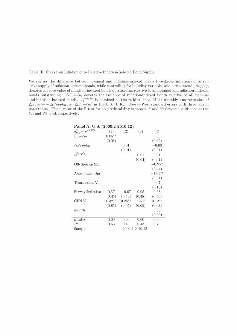
7/29/2019 Return Predictability in the Treasury Market: Real Rates, Inflation, and Liquidity
http://slidepdf.com/reader/full/return-predictability-in-the-treasury-market-real-rates-inflation-and-liquidity 57/91
Table III: Breakeven Inflation onto Relative Inflation-Indexed Bond Supply.
We regress the difference between nominal and inflation-indexed yields (breakeven inflation) onto rel-ative supply of inflation-indexed bonds, while controlling for liquidity variables and a time trend. Supplytdenotes the face value of inflation-indexed bonds outstanding relative to all nominal and inflation-indexedbonds outstanding. ΔSupplyt denotes the issuance of inflation-indexed bonds relative to all nominaland inflation-indexed bonds. ε
Supplyt is obtained as the residual in a 12-lag monthly autoregression of
ΔSupplyt − ΔSupplyt−12 (ΔSupplyt) in the U.S. (U.K.). Newey-West standard errors with three lags inparentheses. The p-value of the F-test for no predictability is shown. * and ** denote significance at the5% and 1% level, respectively.
Panel A: U.S. (2000.2-2010.12)
y$n,t − yTIPS n,t (1) (2) (3) (4)Supplyt 0.05∗∗ 0.03
(0.01) (0.02)ΔSupplyt 0.01 −0.00
(0.01) (0.01)
εSupplyt 0.01 0.01
(0.01) (0.01)Off-the-run Spr. −0.95∗
(0.44)Asset-Swap-Spr. −1.05∗∗
(0.31)Transaction Vol. 0.07
(0.16)Survey Inflation 0.57 −0.07 0.05 0.68
(0.45) (0.49) (0.48) (0.56)CFNAI 0.32∗∗ 0.26∗∗ 0.27∗∗ 0.12∗∗
(0.05) (0.05) (0.05) (0.03)month 0.00
(0.00)p-value 0.00 0.00 0.00 0.00R2 0.53 0.43 0.43 0.70Sample 2000.2-2010.12

7/29/2019 Return Predictability in the Treasury Market: Real Rates, Inflation, and Liquidity
http://slidepdf.com/reader/full/return-predictability-in-the-treasury-market-real-rates-inflation-and-liquidity 58/91
Table III (continued)
Panel B: U.K. (1986.1-2010.12 and 1999.11-2010.12)
y$n,t− yTIPS
n,t(1) (2) (3) (4) (5)
Supplyt 0.07∗ 0.03 0.01(0.03) (0.03) (0.03)
ΔSupplyt 0.00 −0.00 −0.02(0.02) (0.05) (0.05)
εSupplyt 0.01 0.00 0.02
(0.02) (0.05) (0.05)Off-the-run Spr. −0.11
(0.11)LIBOR-GC Spr. 0.02
(0.03)Transaction Vol. −0.00∗∗
(0.00)
Survey Inflation 0.11∗∗
0.14∗∗
0.14∗∗
0.04∗∗
0.06∗∗
(0.02) (0.01) (0.01) (0.02) (0.02)month 0.01∗∗ 0.01∗∗
(0.00) (0.00)p-value 0.00 0.00 0.00 0.00 0.00R2 0.54 0.51 0.51 0.87 0.88Sample 1986.1− 2010.12 1999.11− 2010.12
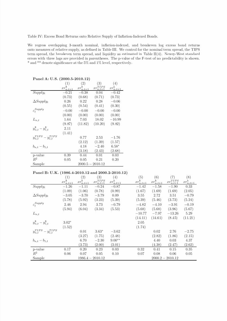
7/29/2019 Return Predictability in the Treasury Market: Real Rates, Inflation, and Liquidity
http://slidepdf.com/reader/full/return-predictability-in-the-treasury-market-real-rates-inflation-and-liquidity 59/91
Table IV: Excess Bond Returns onto Relative Supply of Inflation-Indexed Bonds.
We regress overlapping 3-month nominal, inflation-indexed, and breakeven log excess bond returnsonto measures of relative supply, as defined in Table III. We control for the nominal term spread, the TIPSterm spread, the breakeven term spread, and liquidity as estimated in Table II(4). Newey-West standarderrors with three lags are provided in parentheses. The p-value of the F-test of no predictability is shown.* and ** denote significance at the 5% and 1% level, respectively.
Panel A: U.S. (2000.5-2010.12)(1) (2) (3) (4)
xr$n,t+1 xr$n,t+1 xrTIPS n,t+1 xrbn,t+1Supplyt −0.21 −0.38 0.04 −0.42
(0.73) (0.68) (0.71) (0.73)ΔSupplyt 0.26 0.22 0.28 −0.06
(0.55) (0.54) (0.41) (0.30)
εSupply
t−
0.00
−
0.00
−
0.00
−
0.00(0.00) (0.00) (0.00) (0.00)
Ln,t 1.64 7.03 18.02 −10.99(9.87) (11.82) (10.20) (9.82)
y$n,t − y$1,t 2.11(1.41)
yTIPS n,t − yTIPS 1,t 0.77 2.53 −1.76(2.12) (1.39) (1.57)
bn,t − b1,t 4.18 −2.40 6.58∗
(3.18) (2.43) (2.68)p-value 0.39 0.44 0.01 0.03R2 0.05 0.05 0.21 0.20Sample 2000.5− 2010.12
Panel B: U.K. (1986.4-2010.12 and 2000.2-2010.12)(1) (2) (3) (4) (5) (6) (7) (8)
xr$n,t+1 xr$n,t+1 xrTIPS n,t+1 xrbn,t+1 xr$n,t+1 xr$n,t+1 xrTIPS n,t+1 xrbn,t+1Supplyt −1.26 −1.11 −0.24 −0.87 −1.42 −1.58 −1.90 0.33
(1.09) (1.06) (0.78) (0.99) (1.67) (1.69) (1.69) (2.05)ΔSupplyt −3.05 −3.70 −3.79 0.09 3.55 2.72 3.51 −0.79
(5.78) (5.92) (3.23) (5.39) (5.39) (5.46) (3.73) (5.24)
εSupplyt 2.46 2.94 3.73 −0.79 −4.82 −4.10 −3.91 −0.19
(5.94) (6.04) (3.34) (5.53) (5.68) (5.68) (3.96) (5.67)Ln,t −10.77 −7.97 −13.26 5.29
(14.11) (14.61) (8.45) (11.21)y$n,t − y$1
,t
3.02∗ 2.05(1.52) (1.74)
yTIPS n,t − yTIPS 1,t 0.01 3.63∗ −3.62 0.02 2.76 −2.75(3.27) (1.75) (2.48) (2.82) (1.86) (2.15)
bn,t − b1,t 6.70 −2.30 9.00∗∗ 4.40 0.03 4.37(3.73) (2.00) (3.01) (4.38) (2.47) (2.62)
p-value 0.17 0.20 0.23 0.03 0.32 0.41 0.15 0.35R2 0.06 0.07 0.05 0.10 0.07 0.08 0.06 0.05Sample 1986.4− 2010.12 2000.2− 2010.12
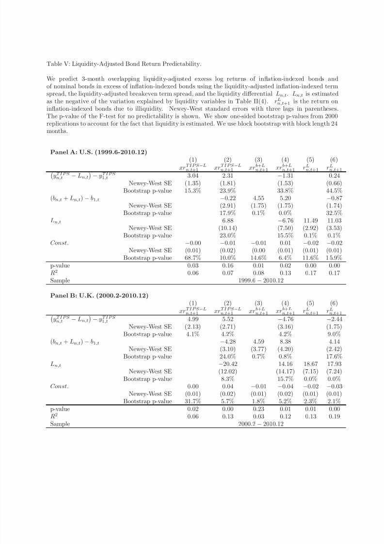
7/29/2019 Return Predictability in the Treasury Market: Real Rates, Inflation, and Liquidity
http://slidepdf.com/reader/full/return-predictability-in-the-treasury-market-real-rates-inflation-and-liquidity 60/91
Table V: Liquidity-Adjusted Bond Return Predictability.
We predict 3-month overlapping liquidity-adjusted excess log returns of inflation-indexed bonds andof nominal bonds in excess of inflation-indexed bonds using the liquidity-adjusted inflation-indexed term
spread, the liquidity-adjusted breakeven term spread, and the liquidity differential Ln,t. Ln,t is estimatedas the negative of the variation explained by liquidity variables in Table II(4). rLn,t+1 is the return oninflation-indexed bonds due to illiquidity. Newey-West standard errors with three lags in parentheses.The p-value of the F-test for no predictability is shown. We show one-sided bootstrap p-values from 2000replications to account for the fact that liquidity is estimated. We use block bootstrap with block length 24months.
Panel A: U.S. (1999.6-2010.12)(1) (2) (3) (4) (5) (6)
xrTIPS −Ln,t+1 xrTIPS −Ln,t+1 xrb+Ln,t+1 xrb+Ln,t+1 rLn,t+1 rLn,t+1yTIPS n,t − Ln,t
− yTIPS 1,t 3.04 2.31 −1.31 0.24
Newey-West SE (1.35) (1.81) (1.53) (0.66)
Bootstrap p-value 15.3% 23.9% 33.8% 44.5%(bn,t + Ln,t)− b1,t −0.22 4.55 5.20 −0.87
Newey-West SE (2.91) (1.75) (1.75) (1.74)Bootstrap p-value 17.9% 0.1% 0.0% 32.5%
Ln,t 6.88 −6.76 11.49 11.03Newey-West SE (10.14) (7.50) (2.92) (3.53)
Bootstrap p-value 23.0% 15.5% 0.1% 0.1%Const. −0.00 −0.01 −0.01 0.01 −0.02 −0.02
Newey-West SE (0.01) (0.02) (0.00 (0.01) (0.01) (0.01)Bootstrap p-value 68.7% 10.0% 14.6% 6.4% 11.6% 1 5.9%
p-value 0.03 0.16 0.01 0.02 0.00 0.00R2 0.06 0.07 0.08 0.13 0.17 0.17Sample 1999.6− 2010.12
Panel B: U.K. (2000.2-2010.12)(1) (2) (3) (4) (5) (6)
xrTIPS −Ln,t+1 xrTIPS −Ln,t+1 xrb+Ln,t+1 xrb+Ln,t+1 rLn,t+1 rLn,t+1yTIPS n,t − Ln,t
− yTIPS 1,t 4.99 5.52 −4.76 −2.44
Newey-West SE (2.13) (2.71) (3.16) (1.75)Bootstrap p-value 4.1% 4.2% 4.2% 9.0%
(bn,t + Ln,t)− b1,t −4.28 4.59 8.38 4.14Newey-West SE (3.10) (3.77) (4.20) (2.42)
Bootstrap p-value 24.0% 0.7% 0.8% 17.6%Ln,t −20.42 14.16 18.67 17.93
Newey-West SE (12.02) (14.17) (7.15) (7.24)
Bootstrap p-value 8.3% 15.7% 0.0% 0.0%Const. 0.00 0.04 −0.01 −0.04 −0.02 −0.03Newey-West SE (0.01) (0.02) (0.01) (0.02) (0.01) (0.01)
Bootstrap p-value 31.7% 5.7% 1.8% 5.2% 2.3% 2.1%p-value 0.02 0.00 0.23 0.01 0.01 0.00R2 0.06 0.13 0.03 0.12 0.13 0.19Sample 2000.2− 2010.12

7/29/2019 Return Predictability in the Treasury Market: Real Rates, Inflation, and Liquidity
http://slidepdf.com/reader/full/return-predictability-in-the-treasury-market-real-rates-inflation-and-liquidity 61/91
Table VI: Predicted Bond Returns.
We show summary statistics for 3-month overlapping log excess returns on real bonds and breakeven, andfor average log liquidity returns. Realized log excess returns are denoted xrn,t, while predicted returns are
denoted E t (xrn,t+1). We show realized sample average returns E (xrn,t) and stock-market betas β (xrn,t).Betas are with respect to excess log stock returns including dividends. We obtain predicted excess returns as
as fitted values from the regressions shown in Tables V(1), V(3) and V(5). Numbers shown are annualized(%). Newey-West standard errors for β are computed with three lags. * and ** denote significance at the
5% and 1% level for β , respectively.
Panel A: U.S. (1999.6-2010.12) Sample Average Stock Market Beta Std. Predicted Exc. Return
E (xrn,t) β (xrn,t) σ (E txrn,t+1)
Liq.-Adj. Exc. Log Ret. BEI 0.52 −0.08 1.62Liq.-Adj. Exc. Log Ret. TIPS 3.67 −0.11 1.63Log Return Liquidity 0.99 0.12∗∗ 1.41
Panel B: U.K. (2000.2-2010.12) Sample Average Stock Market Beta Std. Predicted Exc. Return
E (xrn,t) β (xrn,t) σ (E txrn,t+1)
Liq.-Adj. Exc. Log Ret. BEI −0.34 −0.22∗ 1.93Liq.-Adj. Exc. Log Ret. TIPS 0.85 0.14 2.61Log Return Liquidity 1.61 −0.03 2.23

7/29/2019 Return Predictability in the Treasury Market: Real Rates, Inflation, and Liquidity
http://slidepdf.com/reader/full/return-predictability-in-the-treasury-market-real-rates-inflation-and-liquidity 62/91
Panel A: U.S. (1999.3-2010.12)
- 1 . 5
- 1
- . 5
0
T r a n s a c t i o n V o l .
0
. 5
1
1 . 5
A n n u a l i z e d ( % )
99 00 01 02 03 04 05 06 07 08 09 10Year
Off-the-Run Spread Asset-Swap Spread
Synthetic Minus Cash Transaction Vol. (Right)
Panel B: U.K. (1999.11-2010.12)
- 1 . 5
- 1
- . 5
0
T r a n s a c t i o n
V o l .
0
. 5
1
1 . 5
2
2 . 5
A n n u a l i z e d
( % )
99 00 01 02 03 04 05 06 07 08 09 10Year
Off-the-Run Spread LIBOR-GC Spread
Transaction Vol. (Right)
Figure 1: U.S. and U.K. Liquidity Proxies.
We use liquidity proxies to estimate differential liquidity between inflation-indexedand nominal government bonds. For the U.S., we use the spread between off-the-run andon-the-run 10 year nominal bond yields, the relative inflation-indexed bond log transactionvolume, the asset-swap differential, and the difference between synthetic and cash breakeven.For the U.K., we use the the difference between a 10 year nominal fitted par yield and the10 year nominal generic Bloomberg yield, denoted “off the run”. We normalize the maximaof relative transaction volumes to zero. The asset-swap spread differential, synthetic minus
cash breakeven, and the GBP three-month LIBOR-GC spread proxy for the cost of fundinga levered investment in inflation-indexed bonds.

7/29/2019 Return Predictability in the Treasury Market: Real Rates, Inflation, and Liquidity
http://slidepdf.com/reader/full/return-predictability-in-the-treasury-market-real-rates-inflation-and-liquidity 63/91
Panel A: U.S. (1999.3-2010.12)
- . 5
0
. 5
1
1 . 5
2
A n n u a l i z e d ( % )
99 00 01 02 03 04 05 06 07 08 09 10
Year
Panel B: U.K. (1999.11-2010.12)
- . 5
0
. 5
1
1
. 5
2
A n n u a l i z e d ( % )
99 00 01 02 03 04 05 06 07 08 09 10year
Figure 2: Estimated U.S. and U.K. Liquidity Premia.
We estimate liquidity premia as the negative of the variation in breakeven explainedby liquidity proxies. Formally, Ln,t = −a2X t, where X t is the vector of liquidity variablesand a2 is the vector of corresponding estimated coefficients in Table II(4), Panels A and B.

7/29/2019 Return Predictability in the Treasury Market: Real Rates, Inflation, and Liquidity
http://slidepdf.com/reader/full/return-predictability-in-the-treasury-market-real-rates-inflation-and-liquidity 64/91
Panel A: U.S. (1999.3-2010.12)
0
. 5
1
1 . 5
2
2 . 5
3
3 . 5
4
4 . 5
A n n u a l i z e d ( % )
99 00 01 02 03 04 05 06 07 08 09 10Year
U.S. Breakeven Liquidity-Adjusted U.S. Breakeven
Panel B: U.K. (1999.11-2010.12)
0
. 5
1
1 . 5
2
2 . 5
3
3
. 5
4
4 . 5
A n n u a l i z e d ( % )
99 00 01 02 03 04 05 06 07 08 09 10Year
U.K. Breakeven Liquidity-Adjusted U.K. Breakeven
Figure 3: Liquidity-Adjusted U.S. 10 Year Breakeven and U.K. 20 Year Breakeven.
Liquidity-adjusted breakeven equals breakeven plus the liquidity premium shown inFigure 2.

7/29/2019 Return Predictability in the Treasury Market: Real Rates, Inflation, and Liquidity
http://slidepdf.com/reader/full/return-predictability-in-the-treasury-market-real-rates-inflation-and-liquidity 65/91
Panel A: U.S. (2000.2-2010.12)
0
5
1 0
1 5
( % )
. 5
1
1 . 5
2
2 . 5
3
A n n u a l i z e d ( % )
99 00 01 02 03 04 05 06 07 08 09 10Year
U.S. Breakeven Relative Supply U.S. TIPS (Right)
Panel B: U.K. (1986.1-2010.12)
1 0
1 5
2 0
( % )
2
3
4
5
6
A n n u a l i z e d ( % )
85 90 95 00 05 10year
Breakeven Relative Supply Linkers (Right)
Figure 4: Relative Supply of Inflation-Indexed Bonds and Breakeven.
Relative supply shows the face value of inflation-indexed bonds outstanding relativeto the face value of inflation-indexed and nominal bonds outstanding. We show 10 yearU.S. breakeven and 20 year U.K. breakeven.

7/29/2019 Return Predictability in the Treasury Market: Real Rates, Inflation, and Liquidity
http://slidepdf.com/reader/full/return-predictability-in-the-treasury-market-real-rates-inflation-and-liquidity 66/91
Panel A: U.S. (1999.6-2010.12)
- 5
0
5
1 0
1 5
A n n u a l i z e d ( % )
99 00 01 02 03 04 05 06 07 08 09 10Year
U.S. Liquidity RP U.S. Real Rate RP
U.S. Inflation RP
Panel B: U.K. (2000.2-2010.12)
- 1 0
- 5
0
5
1 0
1 5
A n n u a l i z e d ( % )
99 00 01 02 03 04 05 06 07 08 09 10Year
U.K. Liquidity RP U.K. Real Rate RP
U.K. Inflation RP
Figure 5: U.S. and U.K. Estimated Risk Premia.
Predicted 3-month excess returns in annualized units, labeled real rate risk premia,inflation risk premia, and liquidity risk premia. We obtain predicted excess returns as fitted
values from the regressions shown in Tables V(1), V(3) and V(5), Panels A and B.

7/29/2019 Return Predictability in the Treasury Market: Real Rates, Inflation, and Liquidity
http://slidepdf.com/reader/full/return-predictability-in-the-treasury-market-real-rates-inflation-and-liquidity 67/91
Table I: Summary Statistics.
Nominal and inflation-indexed bond yields, excess returns, inflation expectation proxies, and liquid-ity proxies. U.S. 10 year nominal and TIPS yields from Gurkaynak, Sack, and Wright (2010). U.K.20 year nominal and inflation-indexed yields from Anderson and Sleath (2001). U.S. three-month logexcess returns (1996.-2010.12) and U.K. three-month log excess returns (2000.2-2010.12) are approximatedusing zero-coupon log yields. U.S. survey inflation is the median 10 year CPI inflation forecast from theSurvey of Professional Forecasters. The Chicago Fed National Activity Index (CFNAI) is as in Stock andWatson (1999). U.K. survey inflation reflects Bank of England Public Attitudes Survey 12 month inflationexpectations. U.S. asset-swap spread (2004.1-2010.12), U.S. difference between synthetic and cash breakeven(2004.7-2010.12), and U.K. 3-month GBP LIBOR minus general collateral (GC) spread capture cost of arbitraging between nominal and inflation-indexed bonds. We normalize the maxima of relative transactionvolumes to zero. The U.K. off-the-run spread reflects the spread between a fitted 10 year nominal paryield and the generic 10 year nominal U.K. bond yield from Bloomberg. Spreads and zero-coupon yields
continuously compounded in annualized percent.
Panel A: U.S. (1999.3-2010.12) Mean Std Min Max
Nominal Yields y$n,t 4.68 0.87 2.66 6.70Inflation-Indexed Yields yTIPS n,t 2.44 0.91 0.59 4.29Breakeven bn,t 2.24 0.39 0.39 2.87
Nominal Excess Ret. xr$n,t+1 4.19 8.75 −41.89 56.62Infl.-Indexed Excess Ret. xrTIPS n,t+1 4.66 7.63 −64.91 58.03Breakeven Excess Ret. xrbn,t+1 −0.48 7.30 −42.62 74.33
Survey Inflation πE 2.47 0.07 2.2 2.55Chicago Fed Nat. Activity CFNAI −0.37 0.96 −4.46 1.08Off-the-Run Spr. 0.21 0.11 0.07 0.63
Log Transaction Vol.−
0.57 0.44−
1.44 0.00Asset-Swap Spr. 0.43 0.21 0.21 1.34Synthetic - Cash 0.32 0.17 0.11 1.13
Panel B: U.K. (1999.11-2010.12) Mean Std Min Max
Nominal Yields y$n,t 4.41 0.25 3.79 5.01Inflation-Indexed Yields yTIPS n,t 1.53 0.52 0.57 2.44Breakeven bn,t 2.88 0.46 2.14 3.95
Nominal Excess Ret. xr$n,t+1 0.50 10.09 −49.25 50.08Infl.-Indexed Excess Ret. xrTIPS n,t+1 2.46 8.39 −65.78 32.85Breakeven Excess Ret. xrbn,t+1 −1.96 7.96 −37.39 66.96
Survey Inflation πE
2.52 0.57 1.50 4.40Off-the-Run Spr. 0.04 0.05 −0.06 0.32Log Transaction Vol. −0.65 0.29 −1.36 0.00LIBOR-GC Spr. 0.35 0.36 0.11 2.25

7/29/2019 Return Predictability in the Treasury Market: Real Rates, Inflation, and Liquidity
http://slidepdf.com/reader/full/return-predictability-in-the-treasury-market-real-rates-inflation-and-liquidity 68/91
Table II: Estimating Differential Liquidity.
We regress the difference between nominal and inflation-indexed bond yields (breakeven inflation)onto liquidity proxies. The variables are as described in Table I. Newey-West standard errors with threelags in parentheses. The p-value of the F-test for no predictability is shown. * and ** denote significance atthe 5% and 1% level, respectively.
Panel A: U.S. (1999.3-2010.12)
y$n,t − yTIPS n,t (1) (2) (3) (4) (5) (6) (7)
Off-the-Run Spr. −2.07∗∗ −1.97∗∗ −0.87∗ −1.27∗∗ −1.46∗∗
(0.26) (0.26) (0.42) (0.32) (0.42)Asset-Swap Spr. −0.27 −0.86∗∗ 0.78
(0.24) (0.31) (0.93)Transaction Vol. 0.33∗∗ 0.24∗∗ 0.09
(0.10) (0.07) (0.09)Synthetic-Cash −1.13∗∗
(0.28)Survey Inflation 0.04 0.70 0.50 0.17 0.56 0.80 0.29
(0.46) (0.49) (0.49) (0.41) (0.39) (1.62) (0.82)CFNAI 0.25∗∗ 0.11∗∗ 0.08∗∗ 0.12∗∗ 0.10∗∗ 0.28∗∗ 0.18∗∗
(0.05) (0.04) (0.04) (0.03) (0.03) (0.05) (0.04)p-value 0.00 0.00 0.00 0.00 0.00 0.00 0.00R2 0.39 0.60 0.61 0.66 0.70 0.30 0.61ADF of Residuals −4.17∗∗ −4.45∗∗ −4.27∗∗ −4.73∗∗ −5.08∗∗ −4.58∗∗ −4.75∗∗
Period Full Full Full Full Full 1999.3− 2006.12
Panel B: U.K. (1999.11-2010.12)
y$n,t − yTIPS n,t (1) (2) (3) (4) (5) (6)
Off-the-Run Spr. −0.45 −0.89 −1.25 −3.19∗∗
(0.88) (1.14) (0.94) (0.57)LIBOR-GC Spr. 0.16 0.18 0.39
(0.20) (0.18) (0.20)Transaction Vol. 0.78∗∗ 0.47∗∗
(0.17) (0.11)Survey Inflation 0.57∗∗ 0.59∗∗ 0.56∗∗ 0.28∗∗ 0.55∗∗ 0.27∗∗
(0.06) (0.06) (0.06) (0.08) (0.12) (0.08)p-value 0.00 0.00 0.00 0.00 0.00 0.00
R2
0.51 0.51 0.52 0.65 0.31 0.67ADF of Residuals −3.86∗ −3.88∗ −3.92∗ −4.14∗∗ −3.88∗ −4.07∗∗
Period Full Full Full Full 1999.11− 2006.12

7/29/2019 Return Predictability in the Treasury Market: Real Rates, Inflation, and Liquidity
http://slidepdf.com/reader/full/return-predictability-in-the-treasury-market-real-rates-inflation-and-liquidity 69/91
Table III: Breakeven Inflation onto Relative Inflation-Indexed Bond Supply.
We regress the difference between nominal and inflation-indexed yields (breakeven inflation) onto rel-ative supply of inflation-indexed bonds, while controlling for liquidity variables and a time trend. Supplytdenotes the face value of inflation-indexed bonds outstanding relative to all nominal and inflation-indexedbonds outstanding. ΔSupplyt denotes the issuance of inflation-indexed bonds relative to all nominaland inflation-indexed bonds. ε
Supplyt is obtained as the residual in a 12-lag monthly autoregression of
ΔSupplyt − ΔSupplyt−12 (ΔSupplyt) in the U.S. (U.K.). Newey-West standard errors with three lags inparentheses. The p-value of the F-test for no predictability is shown. * and ** denote significance at the5% and 1% level, respectively.
Panel A: U.S. (2000.2-2010.12)
y$n,t − yTIPS n,t (1) (2) (3) (4)Supplyt 0.05∗∗ 0.03
(0.01) (0.02)ΔSupplyt 0.01 −0.00
(0.01) (0.01)
εSupplyt 0.01 0.01
(0.01) (0.01)Off-the-run Spr. −0.95∗
(0.44)Asset-Swap-Spr. −1.05∗∗
(0.31)Transaction Vol. 0.07
(0.16)Survey Inflation 0.57 −0.07 0.05 0.68
(0.45) (0.49) (0.48) (0.56)CFNAI 0.32∗∗ 0.26∗∗ 0.27∗∗ 0.12∗∗
(0.05) (0.05) (0.05) (0.03)month 0.00
(0.00)p-value 0.00 0.00 0.00 0.00R2 0.53 0.43 0.43 0.70Sample 2000.2-2010.12
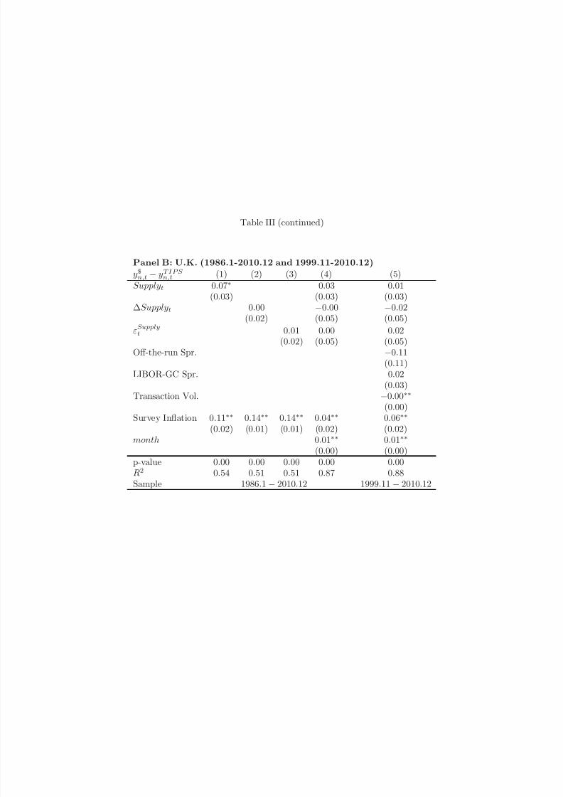
7/29/2019 Return Predictability in the Treasury Market: Real Rates, Inflation, and Liquidity
http://slidepdf.com/reader/full/return-predictability-in-the-treasury-market-real-rates-inflation-and-liquidity 70/91
Table III (continued)
Panel B: U.K. (1986.1-2010.12 and 1999.11-2010.12)
y$n,t− yTIPS
n,t(1) (2) (3) (4) (5)
Supplyt 0.07∗ 0.03 0.01(0.03) (0.03) (0.03)
ΔSupplyt 0.00 −0.00 −0.02(0.02) (0.05) (0.05)
εSupplyt 0.01 0.00 0.02
(0.02) (0.05) (0.05)Off-the-run Spr. −0.11
(0.11)LIBOR-GC Spr. 0.02
(0.03)Transaction Vol. −0.00∗∗
(0.00)
Survey Inflation 0.11∗∗
0.14∗∗
0.14∗∗
0.04∗∗
0.06∗∗
(0.02) (0.01) (0.01) (0.02) (0.02)month 0.01∗∗ 0.01∗∗
(0.00) (0.00)p-value 0.00 0.00 0.00 0.00 0.00R2 0.54 0.51 0.51 0.87 0.88Sample 1986.1− 2010.12 1999.11− 2010.12

7/29/2019 Return Predictability in the Treasury Market: Real Rates, Inflation, and Liquidity
http://slidepdf.com/reader/full/return-predictability-in-the-treasury-market-real-rates-inflation-and-liquidity 71/91
Table IV: Excess Bond Returns onto Relative Supply of Inflation-Indexed Bonds.
We regress overlapping 3-month nominal, inflation-indexed, and breakeven log excess bond returnsonto measures of relative supply, as defined in Table III. We control for the nominal term spread, the TIPSterm spread, the breakeven term spread, and liquidity as estimated in Table II(4). Newey-West standarderrors with three lags are provided in parentheses. The p-value of the F-test of no predictability is shown.* and ** denote significance at the 5% and 1% level, respectively.
Panel A: U.S. (2000.5-2010.12)(1) (2) (3) (4)
xr$n,t+1 xr$n,t+1 xrTIPS n,t+1 xrbn,t+1Supplyt −0.21 −0.38 0.04 −0.42
(0.73) (0.68) (0.71) (0.73)ΔSupplyt 0.26 0.22 0.28 −0.06
(0.55) (0.54) (0.41) (0.30)
εSupply
t−
0.00
−
0.00
−
0.00
−
0.00(0.00) (0.00) (0.00) (0.00)
Ln,t 1.64 7.03 18.02 −10.99(9.87) (11.82) (10.20) (9.82)
y$n,t − y$1,t 2.11(1.41)
yTIPS n,t − yTIPS 1,t 0.77 2.53 −1.76(2.12) (1.39) (1.57)
bn,t − b1,t 4.18 −2.40 6.58∗
(3.18) (2.43) (2.68)p-value 0.39 0.44 0.01 0.03R2 0.05 0.05 0.21 0.20Sample 2000.5− 2010.12
Panel B: U.K. (1986.4-2010.12 and 2000.2-2010.12)(1) (2) (3) (4) (5) (6) (7) (8)
xr$n,t+1 xr$n,t+1 xrTIPS n,t+1 xrbn,t+1 xr$n,t+1 xr$n,t+1 xrTIPS n,t+1 xrbn,t+1Supplyt −1.26 −1.11 −0.24 −0.87 −1.42 −1.58 −1.90 0.33
(1.09) (1.06) (0.78) (0.99) (1.67) (1.69) (1.69) (2.05)ΔSupplyt −3.05 −3.70 −3.79 0.09 3.55 2.72 3.51 −0.79
(5.78) (5.92) (3.23) (5.39) (5.39) (5.46) (3.73) (5.24)
εSupplyt 2.46 2.94 3.73 −0.79 −4.82 −4.10 −3.91 −0.19
(5.94) (6.04) (3.34) (5.53) (5.68) (5.68) (3.96) (5.67)Ln,t −10.77 −7.97 −13.26 5.29
(14.11) (14.61) (8.45) (11.21)y$n,t − y$1
,t
3.02∗ 2.05(1.52) (1.74)
yTIPS n,t − yTIPS 1,t 0.01 3.63∗ −3.62 0.02 2.76 −2.75(3.27) (1.75) (2.48) (2.82) (1.86) (2.15)
bn,t − b1,t 6.70 −2.30 9.00∗∗ 4.40 0.03 4.37(3.73) (2.00) (3.01) (4.38) (2.47) (2.62)
p-value 0.17 0.20 0.23 0.03 0.32 0.41 0.15 0.35R2 0.06 0.07 0.05 0.10 0.07 0.08 0.06 0.05Sample 1986.4− 2010.12 2000.2− 2010.12

7/29/2019 Return Predictability in the Treasury Market: Real Rates, Inflation, and Liquidity
http://slidepdf.com/reader/full/return-predictability-in-the-treasury-market-real-rates-inflation-and-liquidity 72/91
Table V: Liquidity-Adjusted Bond Return Predictability.
We predict 3-month overlapping liquidity-adjusted excess log returns of inflation-indexed bonds andof nominal bonds in excess of inflation-indexed bonds using the liquidity-adjusted inflation-indexed term
spread, the liquidity-adjusted breakeven term spread, and the liquidity differential Ln,t. Ln,t is estimatedas the negative of the variation explained by liquidity variables in Table II(4). rLn,t+1 is the return oninflation-indexed bonds due to illiquidity. Newey-West standard errors with three lags in parentheses.The p-value of the F-test for no predictability is shown. We show one-sided bootstrap p-values from 2000replications to account for the fact that liquidity is estimated. We use block bootstrap with block length 24months.
Panel A: U.S. (1999.6-2010.12)(1) (2) (3) (4) (5) (6)
xrTIPS −Ln,t+1 xrTIPS −Ln,t+1 xrb+Ln,t+1 xrb+Ln,t+1 rLn,t+1 rLn,t+1yTIPS n,t − Ln,t
− yTIPS 1,t 3.04 2.31 −1.31 0.24
Newey-West SE (1.35) (1.81) (1.53) (0.66)
Bootstrap p-value 15.3% 23.9% 33.8% 44.5%(bn,t + Ln,t)− b1,t −0.22 4.55 5.20 −0.87
Newey-West SE (2.91) (1.75) (1.75) (1.74)Bootstrap p-value 17.9% 0.1% 0.0% 32.5%
Ln,t 6.88 −6.76 11.49 11.03Newey-West SE (10.14) (7.50) (2.92) (3.53)
Bootstrap p-value 23.0% 15.5% 0.1% 0.1%Const. −0.00 −0.01 −0.01 0.01 −0.02 −0.02
Newey-West SE (0.01) (0.02) (0.00 (0.01) (0.01) (0.01)Bootstrap p-value 68.7% 10.0% 14.6% 6.4% 11.6% 1 5.9%
p-value 0.03 0.16 0.01 0.02 0.00 0.00R2 0.06 0.07 0.08 0.13 0.17 0.17Sample 1999.6− 2010.12
Panel B: U.K. (2000.2-2010.12)(1) (2) (3) (4) (5) (6)
xrTIPS −Ln,t+1 xrTIPS −Ln,t+1 xrb+Ln,t+1 xrb+Ln,t+1 rLn,t+1 rLn,t+1yTIPS n,t − Ln,t
− yTIPS 1,t 4.99 5.52 −4.76 −2.44
Newey-West SE (2.13) (2.71) (3.16) (1.75)Bootstrap p-value 4.1% 4.2% 4.2% 9.0%
(bn,t + Ln,t)− b1,t −4.28 4.59 8.38 4.14Newey-West SE (3.10) (3.77) (4.20) (2.42)
Bootstrap p-value 24.0% 0.7% 0.8% 17.6%Ln,t −20.42 14.16 18.67 17.93
Newey-West SE (12.02) (14.17) (7.15) (7.24)
Bootstrap p-value 8.3% 15.7% 0.0% 0.0%Const. 0.00 0.04 −0.01 −0.04 −0.02 −0.03Newey-West SE (0.01) (0.02) (0.01) (0.02) (0.01) (0.01)
Bootstrap p-value 31.7% 5.7% 1.8% 5.2% 2.3% 2.1%p-value 0.02 0.00 0.23 0.01 0.01 0.00R2 0.06 0.13 0.03 0.12 0.13 0.19Sample 2000.2− 2010.12

7/29/2019 Return Predictability in the Treasury Market: Real Rates, Inflation, and Liquidity
http://slidepdf.com/reader/full/return-predictability-in-the-treasury-market-real-rates-inflation-and-liquidity 73/91
Table VI: Predicted Bond Returns.
We show summary statistics for 3-month overlapping log excess returns on real bonds and breakeven, andfor average log liquidity returns. Realized log excess returns are denoted xrn,t, while predicted returns are
denoted E t (xrn,t+1). We show realized sample average returns E (xrn,t) and stock-market betas β (xrn,t).Betas are with respect to excess log stock returns including dividends. We obtain predicted excess returns as
as fitted values from the regressions shown in Tables V(1), V(3) and V(5). Numbers shown are annualized(%). Newey-West standard errors for β are computed with three lags. * and ** denote significance at the
5% and 1% level for β , respectively.
Panel A: U.S. (1999.6-2010.12) Sample Average Stock Market Beta Std. Predicted Exc. Return
E (xrn,t) β (xrn,t) σ (E txrn,t+1)
Liq.-Adj. Exc. Log Ret. BEI 0.52 −0.08 1.62Liq.-Adj. Exc. Log Ret. TIPS 3.67 −0.11 1.63Log Return Liquidity 0.99 0.12∗∗ 1.41
Panel B: U.K. (2000.2-2010.12) Sample Average Stock Market Beta Std. Predicted Exc. Return
E (xrn,t) β (xrn,t) σ (E txrn,t+1)
Liq.-Adj. Exc. Log Ret. BEI −0.34 −0.22∗ 1.93Liq.-Adj. Exc. Log Ret. TIPS 0.85 0.14 2.61Log Return Liquidity 1.61 −0.03 2.23

7/29/2019 Return Predictability in the Treasury Market: Real Rates, Inflation, and Liquidity
http://slidepdf.com/reader/full/return-predictability-in-the-treasury-market-real-rates-inflation-and-liquidity 74/91
Appendix: Return Predictability in the Treasury Market:
Real Rates, Inflation, and Liquidity
Carolin E. Pflueger and Luis M. Viceira1
First draft: July 2010This version: April 2013
1Pflueger: University of British Columbia, Vancouver BC V6T 1Z2, Canada. Email [email protected]. Viceira:
Harvard Business School, Boston MA 02163 and NBER. Email [email protected]. We thank Tom Powers and Haibo Jiang
for excellent research assistance. We are grateful to John Campbell, Kent Daniel, Graig Fantuzzi, Michael Fleming, Josh
Gottlieb, Robin Greenwood, Arvind Krishnamurthy, George Pennacchi, Michael Pond, Matthew Richardson, Jeremy Stein, to
seminar participants at the NBER Summer Institute 2011, the Econometric Society Winter Meeting 2011, the Federal Reserve
Board, the European Central Bank, the New York Federal Reserve, the Foster School of Business at the U. of Washington,
the HBS-Harvard Economics Finance Lunch and the HBS Finance Research Day for helpful comments and suggestions. We
are also grateful to Martin Duffell and Anna Christie from the U.K. Debt Management Office for their help providing us with
U.K. bond data. This material is based upon work supported by the Harvard Business School Research Funding. This paper
was previously circulated under the title “An Empirical Decomposition of Risk and Liquidity in Nominal and Inflation-Indexed
Government Bonds”.

7/29/2019 Return Predictability in the Treasury Market: Real Rates, Inflation, and Liquidity
http://slidepdf.com/reader/full/return-predictability-in-the-treasury-market-real-rates-inflation-and-liquidity 75/91
Table A.I: Forecasted Real Short Rate.
Overlapping quarterly realized real return on nominal three month T-bill onto the nominal three
month T-bill, three month lagged realized real return on three month T-bill and inflation over the past year.Newey-West standard errors with four lags in parentheses. * and ** denote significance at the 5% and 1%level.
(1) (2)
y$1,t − πt+1 U.S. UK
y$1,t 0.55∗∗ 0.79∗∗
(0.20) (0.13)y$1,t − πt 0.10 −0.08
(0.08) (0.05)(πt−3 + πt−2 + πt−1 + πt) /4 0.10 −0.07
(0.08) (0.04)
Const. −0.52∗∗ −0.26∗
(0.09) (0.12)p-value 0.00 0.00R2 0.48 0.48Sample 1982.1− 2010.12
1

7/29/2019 Return Predictability in the Treasury Market: Real Rates, Inflation, and Liquidity
http://slidepdf.com/reader/full/return-predictability-in-the-treasury-market-real-rates-inflation-and-liquidity 76/91
Table A.II: Univariate Liquidity Regressions
Variables as in Table II. Newey-West standard errors with three lags in parentheses. The p-value of the F-test for no predictability is shown. * and ** denote significance at the 5% and 1% level.
Panel A. U.S. (1999.3− 2010.12)
y$n,t−yTIPS n,t (1) (2) (3) (4) (5) (6)
Off-the-Run Spr. −2.54∗∗
(0.39)Asset-Swap Spr. −1.24∗∗
(0.29)Transaction Vol. 0.19
(0.14)Synthetic-Cash −1.85∗∗
(0.37)Survey Inflation −0.00
(0.51)CFNAI 0.25∗∗
(0.05)p-value 0.00 0.00 0.18 0.00 1.00 0.00R2 0.53 0.32 0.05 0.36 0.00 0.39Sample 1999.3− 2010.12
Panel B: U.K. (1999.11-2010.12)
y$n,t − yTIPS n,t (1) (2) (3) (4)
Off-the-Run Spr. 1.59(1.00)
LIBOR-GC Spr. 0.46∗∗
(0.15)Transaction Vol. 1.17∗∗
(0.13)Survey Inflation 0.57∗∗
(0.06)p-value 0.11 0.00 0.00 0.00
R
2
0.03 0.13 0.56 0.51Period 1999.11− 2006.12
2

7/29/2019 Return Predictability in the Treasury Market: Real Rates, Inflation, and Liquidity
http://slidepdf.com/reader/full/return-predictability-in-the-treasury-market-real-rates-inflation-and-liquidity 77/91
Table A.III: Estimating Liquidity in Quarterly Changes
We replicate Table II using quarterly changes. Newey-West standard errors with three lags in parentheses.The p-value of the F-test for no predictability is shown. * and ** denote significance at the 5% and 1%level.
Panel A: U.S. (1999.6-2010.12)
∆y$n,t−y
TIPS n,t
(1) (2) (3) (4) (5) (6) (7)
∆ Off-the-Run Spr. −2.47∗∗ −1.02∗ −1.02∗ −1.59∗∗ −0.95(0.68) (0.47) (0.47) (0.49) (0.53)
∆ Asset-Swap Spr. −1.24∗∗ −1.24∗∗ 0.55
(0.26) (0.27) (0.76)∆ Transaction Vol. −0.04 −0.09 −0.19
(0.19) (0.19) (0.18)∆ Synthetic-Cash −1.16∗∗
(0.17)∆ Survey Inflation −0.71 −0.34 −0.55 −0.53 −0.62 −0.00 0.24
(0.55) (0.49) (0.50) (0.50) (0.49) (1.14) (1.09)∆ CFNAI 0.16∗∗ 0.10∗∗ 0.09∗∗ 0.09∗∗ 0.08∗∗ 0.05 0.05
(0.05) (0.03) (0.03) (0.03) (0.03) (0.04) (0.04)p-value 0.01 0.00 0.00 0.00 0.00 0.46 0.42R2 0.11 0.37 0.47 0.47 0.48 0.02 0.07Sample 1999.6− 2010.12 1999.6− 2006.12
Panel B: U.K. (2000.2-2010.12)
∆y$n,t−y
TIPS n,t
(1) (2) (3) (4) (5) (6)
∆ Off-the-Run Spr. −0.61 −0.41 −0.20 0.24(0.32) (0.33) (0.34) (0.52)
∆ LIBOR-GC Spr. −0.21∗ −0.22∗∗ 0.42∗
(0.08) (0.08) (0.17)∆ Transaction Vol. −0.17 −0.04
(0.10) (0.08)∆ Survey Inflation 0.18∗ 0.17∗ 0.18∗∗ 0.20∗∗ 0.16∗ 0.21∗∗
(0.08) (0.07) (0.06) (0.05) (0.07) (0.07)p-value 0.02 0.01 0.00 0.00 0.02 0.06
R2
0.13 0.16 0.25 0.27 0.08 0.12Sample 2000.2− 2010.12 2000.2− 2006.12
3

7/29/2019 Return Predictability in the Treasury Market: Real Rates, Inflation, and Liquidity
http://slidepdf.com/reader/full/return-predictability-in-the-treasury-market-real-rates-inflation-and-liquidity 78/91
Table A.IV: Estimating Liquidity with Additional Controls
We replicate Table II including interaction terms and the TIPS bid-ask spread. The TIPS bid-askspread is from Tradeweb and available 2005.3-2010.6. We set to its 2005.3 value before 2005.3 and to its2010.6 value after 2010.6. Newey-West standard errors with three lags in parentheses. The p-value of theF-test for no predictability is shown. * and ** denote significance at the 5% and 1% level.
Panel A. U.S. (1999.3− 2010.12)
y$n,t−yTIPS n,t (1) (2) (3) (4)Off-the-Run Spr. 1.40 1.66 1.50 −0.84
(0.90) (1.05) (1.04) (0.43)Asset-Swap Spr. −0.59∗ −0.67∗ −0.75 −0.65∗
(0.30) (0.31) (0.66) (0.30)Transaction Vol. 0.39∗∗ 0.32 0.39∗∗ 0.32∗∗
(0.11) (0.19) (0.11) (0.10)Survey Inflation 0.22 0.19 0.18 0.02
(0.37) (0.37) (0.34) (0.42)CFNAI 0.14∗∗ 0.14∗∗ 0.14∗∗ 0.12∗∗
(0.04) (0.03) (0.04) (0.03)(Off-the-Run)2 −4.29∗∗ −4.36∗∗ −4.88
(1.53) (1.51) (3.09)Off-the-Run× Transaction Vol. 0.38
(0.79)Off-the-Run× Asset-Swap Spr. 0.46
(1.81)TIPS Bid-Ask Spread −0.34
(0.26)const. 2.15∗ 2.19∗ 2.28∗ 2.87∗∗
(0.96) (0.93) (0.89) (1.06)p-value 0.00 0.00 0.00 0.00R2 0.69 0.69 0.69 0.67Sample 1999.3− 2010.12
4

7/29/2019 Return Predictability in the Treasury Market: Real Rates, Inflation, and Liquidity
http://slidepdf.com/reader/full/return-predictability-in-the-treasury-market-real-rates-inflation-and-liquidity 79/91
Table A.IV (continued)
Panel B. U.K. (1999.11− 2010.12)
y$
n,t−
yTIPS
n,t (1) (2) (3)Off-the-Run Spr. −1.83 −2.02 −0.96(1.43) (2.65) (1.27)
LIBOR-GC Spr. 0.16 0.16 0.60∗∗
(0.17) (0.17) (0.16)Transaction Vol. 0.77∗∗ 0.78∗∗ 0.79∗∗
(0.17) (0.19) (0.18)Survey Inflation 0.29∗∗ 0.30∗∗ 0.27∗∗
(0.08) (0.09) (0.08)(Off-the-Run)2 3.48 3.78 18.96∗∗
(3.94) (5.67) (5.00)Off-the-Run× Transaction Vol. −0.25
(2.26)
Off-the-Run× LIBOR-GC Spr. −5.16∗∗
(1.28)const. 2.65∗∗ 2.64∗∗ 2.59∗∗
(0.33) (0.34) (0.32)p-value 0.00 0.00 0.00R2 0.66 0.66 0.70Sample 1999.3− 2010.12
5

7/29/2019 Return Predictability in the Treasury Market: Real Rates, Inflation, and Liquidity
http://slidepdf.com/reader/full/return-predictability-in-the-treasury-market-real-rates-inflation-and-liquidity 80/91
Table A.V: Nominal Yields onto Liquidity Proxies U.S.
Variables as in Table II. Newey-West standard errors with three lags in parentheses. The p-value of the F-test for no predictability is shown. * and ** denote significance at the 5% and 1% level, respectively.
Panel A: U.S. (1999.3-2010.12)
y$n,t (1) (2) (3) (4) (5) (6) (7)
Off-the-Run Spr. 2.33∗ 3.24∗∗ −0.67 −1.12 −2.45(0.99) (1.00) (1.46) (1.11) (1.48)
Asset-Swap Spr. −2.37∗∗ −0.27 4.21∗
(0.54) (0.78) (2.04)Transaction Vol. −1.17∗∗ −1.27∗∗ −1.81∗∗
(0.30) (0.22) (0.26)Synthetic-Cash 0.52
(0.70)Survey Inflation 5.61∗∗ 4.87∗∗ 3.21∗∗ 4.38∗∗ 4.64∗∗ 1.34 1.18
(1.23) (1.13) (1.06) (1.26) (1.35) (3.16) (1.48)CFNAI 0.28∗∗ 0.44∗∗ 0.21∗ 0.08 0.12 −0.04 0.12
(0.08) (0.11) (0.10) (0.07) (0.07) (0.18) (0.10)p-value 0.00 0.00 0.00 0.00 0.00 0.87 0.00R2 0.30 0.36 0.47 0.60 0.61 0.00 0.63Sample 1999.3− 2010.12 1999.3− 2006.12
Panel B: U.K. (1999.11-2010.12)
y$n,t (1) (2) (3) (4) (5) (6)Off-the-Run Spr. 0.11 −0.16 0.04 2.01∗
(0.57) (0.64) (0.62) (0.91)LIBOR-GC Spr. 0.10 0.09 −1.03∗∗
(0.06) (0.06) (0.28)Transaction Vol. −0.45∗∗ −0.58∗∗
(0.16) (0.16)Survey Inflation 0.02 0.02 0.00 0.16∗ −0.07 0.07
(0.06) (0.06) (0.06) (0.06) (0.19) (0.16)p-value 0.67 0.90 0.35 0.02 0.71 0.00R2 0.00 0.00 0.02 0.16 0.00 0.28
Sample 1999.11− 2010.12 1999.11− 2006.12
6
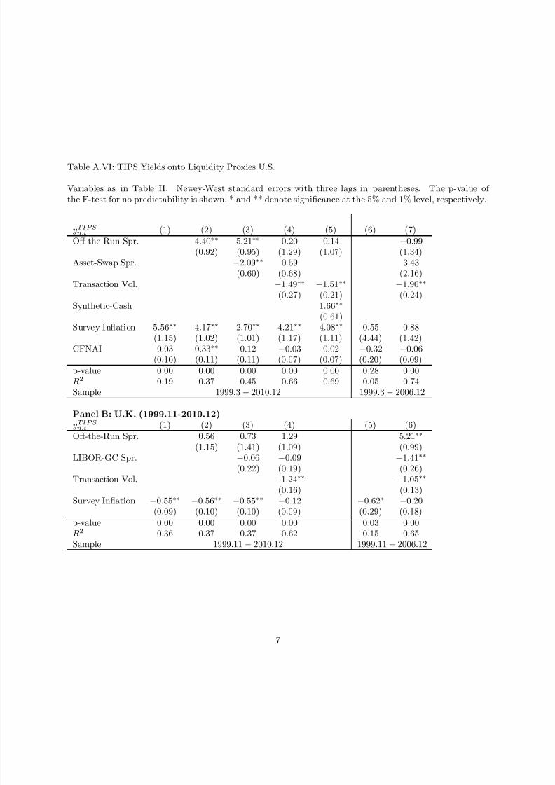
7/29/2019 Return Predictability in the Treasury Market: Real Rates, Inflation, and Liquidity
http://slidepdf.com/reader/full/return-predictability-in-the-treasury-market-real-rates-inflation-and-liquidity 81/91
Table A.VI: TIPS Yields onto Liquidity Proxies U.S.
Variables as in Table II. Newey-West standard errors with three lags in parentheses. The p-value of the F-test for no predictability is shown. * and ** denote significance at the 5% and 1% level, respectively.
yTIPS n,t (1) (2) (3) (4) (5) (6) (7)
Off-the-Run Spr. 4.40∗∗ 5.21∗∗ 0.20 0.14 −0.99(0.92) (0.95) (1.29) (1.07) (1.34)
Asset-Swap Spr. −2.09∗∗ 0.59 3.43
(0.60) (0.68) (2.16)Transaction Vol. −1.49∗∗ −1.51∗∗ −1.90∗∗
(0.27) (0.21) (0.24)Synthetic-Cash 1.66∗∗
(0.61)Survey Inflation 5.56∗∗ 4.17∗∗ 2.70∗∗ 4.21∗∗ 4.08∗∗ 0.55 0.88
(1.15) (1.02) (1.01) (1.17) (1.11) (4.44) (1.42)CFNAI 0.03 0.33∗∗ 0.12 −0.03 0.02 −0.32 −0.06
(0.10) (0.11) (0.11) (0.07) (0.07) (0.20) (0.09)p-value 0.00 0.00 0.00 0.00 0.00 0.28 0.00R2 0.19 0.37 0.45 0.66 0.69 0.05 0.74Sample 1999.3− 2010.12 1999.3− 2006.12
Panel B: U.K. (1999.11-2010.12)yTIPS n,t (1) (2) (3) (4) (5) (6)Off-the-Run Spr. 0.56 0.73 1.29 5.21∗∗
(1.15) (1.41) (1.09) (0.99)LIBOR-GC Spr. −0.06 −0.09 −1.41∗∗
(0.22) (0.19) (0.26)Transaction Vol. −1.24∗∗ −1.05∗∗
(0.16) (0.13)Survey Inflation −0.55∗∗ −0.56∗∗ −0.55∗∗ −0.12 −0.62∗ −0.20
(0.09) (0.10) (0.10) (0.09) (0.29) (0.18)p-value 0.00 0.00 0.00 0.00 0.03 0.00R2 0.36 0.37 0.37 0.62 0.15 0.65Sample 1999.11− 2010.12 1999.11− 2006.12
7

7/29/2019 Return Predictability in the Treasury Market: Real Rates, Inflation, and Liquidity
http://slidepdf.com/reader/full/return-predictability-in-the-treasury-market-real-rates-inflation-and-liquidity 82/91
Table A.VII: Return Predictability Liquidity with Nonlinear Liquidity.
Return-predictability regressions as in Table A.IX. We adjust for nonlinear liquidity as estimated inTable A.IV, column (1) in Panel A and column (3) in Panel B for U.S. and U.K., respectively. Newey-Weststandard errors with three lags appear in parentheses. The p-value of the F-test for no predictability isshown. We also show one-sided bootstrap p-values from 2000 replications. We use block bootstrap withblock length 24 months. Bootstrap accounts for the fact that the liquidity premium is estimated.
Panel A: U.S. (1999.6-2010.12)(1) (2) (3) (4) (5) (6)
xrTIPS −Ln,t+1 xrTIPS −Ln,t+1 xrb+Ln,t+1 xrb+Ln,t+1 rLn,t+1 rLn,t+1yTIPS n,t − Ln,t
− yTIPS 1,t 3.05 2.64 −1.68 −0.29
Newey-West SE (1.24) (1.43) (1.22) (0.53)Bootstrap p-value 12.6% 17.4% 12.8% 28.2%
(bn,t + Ln,t)− b1,t 0.05 4.42 5.11 −0.47Newey-West SE (2.83) (1.62) (1.53) (1.87)
Bootstrap p-value 19.8% 0.1% 0.0% 38.4%Ln,t 4.89 −3.88 15.93 16.38
Newey-West SE (9.20) (5.67) (3.96) (4.18)Bootstrap p-value 26.1% 21.1% 0.0% 0.0%
Const. −0.00 −0.01 −0.00 0.01 −0.01 −0.01Newey-West SE (0.01) (0.01) (0.00) (0.01) (0.01) (0.00)
Bootstrap p-value 73.3% 11.5% 25.6% 7.8% 20.9% 2 6.4%p-value 0.02 0.11 0.01 0.01 0.00 0.00R2 0.06 0.07 0.08 0.12 0.22 0.23Sample 1999.6− 2010.12
Panel B: U.K. (2000.2-2010.12)(1) (2) (3) (4) (5) (6)
xrTIPS −Ln,t+1 xrTIPS −Ln,t+1 xrb+Ln,t+1 xrb+Ln,t+1 rLn,t+1 rLn,t+1yTIPS n,t − Ln,t
− yTIPS 1,t 3.42 2.68 −1.72 0.39
Newey-West SE (2.20) (2.77) (3.10) (2.26)Bootstrap p-value 5.2% 4.6% 5.3% 11.6%
(bn,t + Ln,t)− b1,t −2.50 3.72 6.03 2.41Newey-West SE (3.74) (4.16) (4.60) (2.91)
Bootstrap p-value 23.5% 0.5% 0.8% 19.8%Ln,t −24.17 15.99 21.15 23.20
Newey-West SE (9.51) (11.20) (6.85) (7.94)Bootstrap p-value 7.0% 13.0% 0.0% 0.0%
Const. 0.00 0.03 −0.01 −0.03 −0.02 −0.02Newey-West SE (0.01) (0.01) (0.01) (0.01) (0.01) (0.01)
Bootstrap p-value 31.8% 4.7% 1.7% 3.9% 2.4% 2.1%p-value 0.12 0.00 0.37 0.19 0.00 0.00R2 0.03 0.12 0.02 0.08 0.14 0.16Sample 2000.2− 2010.12
8

7/29/2019 Return Predictability in the Treasury Market: Real Rates, Inflation, and Liquidity
http://slidepdf.com/reader/full/return-predictability-in-the-treasury-market-real-rates-inflation-and-liquidity 83/91
Table A.VIII: Return Predictability Liquidity with Tradeable Excess Returns.
We run liquidity-adjusted return-predictive regressions as in Table A.IX. We consider liquidity-adjustedlog nominal bond returns on TIPS over nominal returns on the nominal T-bill rate rTIPS −Ln,t − rTbillt asa tradeable version of liquidity-adjusted log excess returns of TIPS. We also consider log nominal bondreturns on nominal bonds over liquidity-adjusted log nominal bond returns on TIPS rnomn,t − rTIPS −Ln,t asa tradeable version of liquidity-adjusted breakeven returns. Newey-West standard errors with three lagsappear in parentheses. The p-value of the F-test for no predictability is shown. We also show one-sidedbootstrap p-values from 2000 replications. We use block bootstrap with block length 24 months. Bootstrapaccounts for the fact that the liquidity premium is estimated.
Panel A: U.S. (1999.6-2010.12)
rTIPS −Ln,t − rTbillt
rnomn,t −rTIPS
−Ln,t
yTIPS n,t − Ln,t
−yTIPS 1,t 2.27 2.42 −1.42
Newey-West SE (1.50) (1.69) (1.66)Bootstrap p-value 31.2% 24.3% 33.2%
(bn,t + Ln,t)−b1,t −0.57 4.93 5.55Newey-West SE (2.50) (2.09) (2.20)Bootstrap p-value 14.5% 0.6% 0.2%
Ln,t 5.19 4.91 −7.81 −4.78Newey-West SE (8.75) (9.36) (5.74) (7.58)Bootstrap p-value 21.5% 27.5% 9.8% 20.0%
p-value 0.11 0.20 0.05 0.08R2 0.06 0.06 0.09 0.10
Sample 1999.6−
2010.12
Panel B: U.K. (2000.2-2010.12)
rTIPS −Ln,t − rTbillt
rnomn,t −r
TIPS −Ln,t
yTIPS n,t − Ln,t
−yTIPS 1,t 3.90 4.92 −4.16
Newey-West SE (2.53) (2.71) (3.19)Bootstrap p-value 7.8% 10.4% 13.8%
(bn,t + Ln,t)−b1,t −2.39 3.88 6.49Newey-West SE (2.90) (3.75) (4.22)Bootstrap p-value 14.5% 37.9% 26.0%
Ln,t −17.96 −18.00 15.43 11.74Newey-West SE (12.40) (12.38) (14.32) (15.50)
Bootstrap p-value 62.0% 38.8% 48.3% 50.0%p-value 0.00 0.00 0.39 0.06R2 0.10 0.11 0.05 0.08Sample 2000.2− 2010.12
9

7/29/2019 Return Predictability in the Treasury Market: Real Rates, Inflation, and Liquidity
http://slidepdf.com/reader/full/return-predictability-in-the-treasury-market-real-rates-inflation-and-liquidity 84/91
Table A.IX: Return Predictability of Unadjusted Excess Returns.
We regress 3-month overlapping excess log bond returns of TIPS and of nominal bonds onto theTIPS term spread, the nominal term spread, the liquidity-adjusted TIPS term spread, the liquidity-adjustedbreakeven term spread and the liquidity premium on TIPS Ln,t. Ln,t is estimated as the negative of thevariation explained by liquidity variables in Table II(4). Newey-West standard errors with three lags inparentheses. The p-value of the F-test for no predictability is shown. We also show one-sided bootstrapp-values from 2000 replications. We use block bootstrap with block length 24 months. Bootstrap accountsfor the fact that the liquidity premium is estimated.
Panel A: U.S. (1999.6-2010.12)(1) (2) (3) (4)
xrTIPS n,t+1 xrTIPS n,t+1 xr$n,t+1 xr$n,t+1yTIPS n,t − yTIPS 1,t 4.36
Newey-West SE (1.29)Bootstrap p-value 1.9%
y$n,t − y$1,t 2.40Newey-West SE (1.42)
Bootstrap p-value 21.3%yTIPS n,t − Ln,t
− yTIPS 1,t 2.54 1.00
Newey-West SE (1.71) (2.38)Bootstrap p-value 21.5% 30.8%
(bn,t + Ln,t)− b1,t −1.09 4.98Newey-West SE (2.80) (3.32)
Bootstrap p-value 10.3% 39.3%Ln,t 17.91 0.12
Newey-West SE (8.98) (9.24)Bootstrap p-value 9.2% 48.6%
Const. −0.01 −0.03 −0.00 −0.00Newey-West SE (0.01) (0.01) (0.01) (0.01)
Bootstrap p-value 94.9% 1.9% 46.5% 31.6%p-value 0.00 0.01 0.09 0.33R2 0.12 0.16 0.04 0.05Std-Expected Exc. Ret. 2.64 3.07 1.75 2.01Sample 1999.6− 2010.12
10

7/29/2019 Return Predictability in the Treasury Market: Real Rates, Inflation, and Liquidity
http://slidepdf.com/reader/full/return-predictability-in-the-treasury-market-real-rates-inflation-and-liquidity 85/91
Table A.IX (continued)
Panel B: U.K. (2000.2-2010.12)(1) (2) (3) (4)
xrTIPS n,t+1 xrTIPS n,t+1 xr$n,t+1 xr$n,t+1
yTIPS n,t − y
TIPS 1,t 3.10
Newey-West SE (1.71)Bootstrap p-value 19.5%
y$n,t − y$1,t 2.42Newey-West SE (1.58)
Bootstrap p-value 2.8%yTIPS n,t − Ln,t
− yTIPS 1,t 3.09 0.76
Newey-West SE (1.86) (2.30)Bootstrap p-value 18.0% 41.6%
(bn,t + Ln,t)− b1,t −0.14 4.10Newey-West SE (2.46) (4.37)
Bootstrap p-value 40.2% 3.1%Ln,t −2.49 −6.26
Newey-West SE (10.15) (10.13)Bootstrap p-value 16.3% 26.7%
Const. 0.00 0.01 −0.00 0.00Newey-West SE (0.01) (0.01) (0.01) (0.01)
Bootstrap p-value 52.6% 37.2% 37.3% 48.1%p-value 0.07 0.03 0.13 0.47R2 0.03 0.04 0.04 0.05Std-Expected Exc. Ret. 1.56 1.69 2.01 2.23Sample 2000.2− 2010.12
11
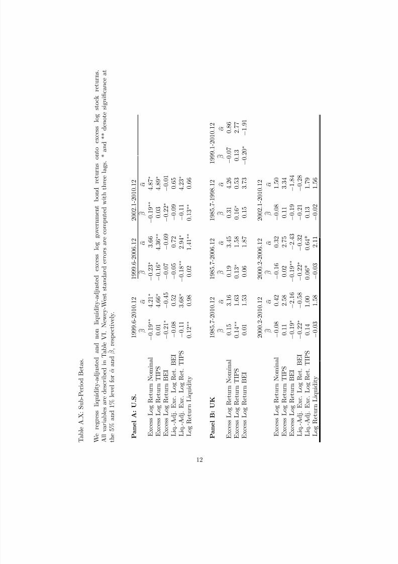
7/29/2019 Return Predictability in the Treasury Market: Real Rates, Inflation, and Liquidity
http://slidepdf.com/reader/full/return-predictability-in-the-treasury-market-real-rates-inflation-and-liquidity 86/91
T a b l e A . X : S u b - P
e r i o d B e t a s .
W e r e g r e s s l i q u i d i t y - a d j u s t e d a n d n o n l i q u i d i t y - a d j u s t e d e x c e s s l o g g o v e r n m e n t b o
n d r e t u r n s o n t o e x c e s s l o g s t o c k
r e t u r n s .
A l l v a r i a b l e s a r e d e s c r i b e d i n T a b l e V I . N e w e y - W e s t s t a n d a r d e r r o r s a r e c o m p u t e d w i t h t h r e e l a g s .
* a n d * * d e n o t e s i g n i fi c a n c e a t
t h e 5 % a n d 1 % l e
v e l f o r ˆ α a n d ˆ β , r e s p e c t i v e l y .
P a n e l A : U . S .
1 9 9 9 . 6 - 2 0 1 0 . 1 2
1 9 9 9 . 6 - 2 0 0 6 . 1 2
2 0 0 2 . 1 - 2 0
1 0 . 1 2
β
α
β
α
β
α
E x c e s s L o g R e t
u r n N o m i n a l
− 0 . 1 9 ∗ ∗
4 . 2 1 ∗
− 0 . 2 3 ∗
3 . 6 6
− 0 . 1 9 ∗ ∗
4 . 8 7 ∗
E x c e s s L o g R e t
u r n T I P S
0 . 0 1
4 . 6 6 ∗
− 0 . 1 6 ∗
4 . 3 6 ∗ ∗
0 . 0 3
4 . 8 9 ∗
E x c e s s L o g R e t
u r n B E I
− 0 . 2 1 ∗
− 0 . 4 5
− 0 . 0 7
− 0 . 6 9
− 0 . 2 2 ∗
− 0 . 0 1
L i q . -
A d j . E x c .
L o g R e t .
B E I
− 0 . 0 8
0 . 5 2
− 0 . 0 5
0 . 7 2
− 0 . 0 9
0 . 6 5
L i q . -
A d j . E x c .
L o g R e t .
T I P S
− 0 . 1 1
3 . 6 8 ∗
− 0 . 1 8 ∗ ∗
2 . 9 4 ∗
− 0 . 1 1
4 . 2 3 ∗
L o g R e t u r n L i q
u i d i t y
0 . 1 2 ∗ ∗
0 . 9 8
0 . 0 2
1 . 4 1 ∗ ∗
0 . 1 3 ∗ ∗
0 . 6 6
P a n e l B : U K
1 9 8 5 . 7 - 2 0 1 0 . 1 2
1 9 8 5 . 7 - 2 0 0 6 . 1 2
1 9 8 5 . 7 - 1 9
9 8 . 1 2
1 9 9 9 . 1 - 2 0 1 0 . 1 2
β
α
β
α
β
α
β
α
E x c e s s L o g R e t u
r n N o m i n a l
0 . 1 5
3 . 1 6
0 . 1 9
3 . 4 5
0 . 3 1
4 . 2 6
− 0 . 0 7
0 . 8 6
E x c e s s L o g R e t u
r n T I P S
0 . 1 4 ∗ ∗
1 . 6 3
0 . 1 3 ∗
1 . 5 8
0 . 1 6 ∗
0 . 5 3
0 . 1 3
2 . 7 7
E x c e s s L o g R e t u
r n B E I
0 . 0 1
1 . 5 3
0 . 0 6
1 . 8 7
0 . 1 5
3 . 7 3
− 0 . 2 0 ∗
− 1 . 9 1
2 0 0 0 . 2 - 2 0 1 0 . 1 2
2 0 0 0 . 2 - 2 0 0 6 . 1 2
2 0 0 2 . 1 - 2 0
1 0 . 1 2
β
α
β
α
β
α
E x c e s s L o g R e t
u r n N o m i n a l
− 0 . 0 8
0 . 4 2
− 0 . 1 6
0 . 3 2
− 0 . 0 8
1 . 5 0
E x c e s s L o g R e t
u r n T I P S
0 . 1 1
2 . 5 8
0 . 0 2
2 . 7 5
0 . 1 1
3 . 3 4
E x c e s s L o g R e t
u r n B E I
− 0 . 1 9 ∗
− 2 . 1 6
− 0 . 1 9 ∗ ∗
− 2 . 4 3
− 0 . 1 9
− 1 . 8 4
L i q . -
A d j . E x c .
L o g R e t .
B E I
− 0 . 2 2 ∗
− 0 . 5 8
− 0 . 2 2 ∗
− 0 . 3 2
− 0 . 2 1
− 0 . 2 8
L i q . -
A d j . E x c .
L o g R e t .
T I P S
0 . 1 4
1 . 0 0
0 . 0 6 *
0 . 6 4 *
0 . 1 3
1 . 7 9
L o g R e t u r n L i q
u i d i t y
− 0 . 0 3
1 . 5 8
− 0 . 0 3
2 . 1 1
− 0 . 0 2
1 . 5 6
12

7/29/2019 Return Predictability in the Treasury Market: Real Rates, Inflation, and Liquidity
http://slidepdf.com/reader/full/return-predictability-in-the-treasury-market-real-rates-inflation-and-liquidity 87/91
Table A.XI: Four Factor Regressions.
US liquidity-adjusted and non liquidity-adjusted excess log government bond returns onto excess log
stock returns xr
equity
t+1 , the SMB factor, the HML factor, and innovations in the Pastor-Stambaugh liquidityfactor. Annualized (%). Newey-West standard errors with three lags in brackets. * and ** denotesignificance at the 5% and 1% level.
Panel A: 1999.6-2010.12 xr$n,t+1 xrTIPS n,t+1 xrbn,t+1 xrTIPS −Ln,t+1 xrb+Ln,t+1 rLn,t+1xrequityt+1 −0.13∗ 0.08 −0.21∗ −0.05 −0.09 0.13∗∗
(0.06) (0.11) (0.09) (0.07) (0.05) (0.04)HML 0.02 −0.03 0.05 −0.04 0.06 0.01
(0.06) (0.07) (0.06) (0.07) (0.06) (0.02)SMB −0.16∗ −0.11 −0.05 −0.13∗ -0.03 0.03
(0.06) (0.06) (0.05) (0.05) (0.05) (0.02)Pastor-Stambaugh −0.07∗ −0.08∗ 0.01 −0.07∗ −0.00 −0.02
(0.03) (0.03) (0.03) (0.03) (0.03) (0.01)const. 5.00∗ 5.23∗∗ −0.22 4.59∗∗ 0.42 0.64
(1.99) (1.81) (1.60) (1.47) (1.30) (0.67)
13

7/29/2019 Return Predictability in the Treasury Market: Real Rates, Inflation, and Liquidity
http://slidepdf.com/reader/full/return-predictability-in-the-treasury-market-real-rates-inflation-and-liquidity 88/91
Table A.XII: Dickey-Fuller Unit Root Tests.
We report Dickey-Fuller test for the null-hypothesis of a unit root with twelve lags. Supplyt denotesthe amount of inflation-indexed bonds outstanding relative to all nominal and inflation-indexed bondsoutstanding. ∆Supplyt denotes the relative issuance of inflation-indexed bonds relative to all nominal andinflation-indexed bonds issuance. ∆Supplyt −∆Supplyt−12 is the change in relative issuance over the past12 months. * and ** denote significance at the 5% and 1% level respectively.
Panel A: U.S.
Supplyt ∆Supplyt ∆Supplyt −∆Supplyt−12−2.02 −2.12 −3.25∗
Sample 1999.1−
2010.12 1999.2−
2010.12 2000.2−
2010.12
Panel B: UK
Supplyt ∆Supplyt ∆Supplyt −∆Supplyt−12−1.96 −4.75∗∗ −2.65
Sample 1986.1− 2010.12 1986.1− 2010.12 1987.1− 2010.12
Table A.XIII: Supply Autoregression.
We regress relative issuance ∆Supplyt, as described in Table 5 onto its own twelve lags. We alsoregress the 12-month change in relative issuance onto its own twelve lags. We report the sum of the twelveautoregressive coefficients.
Panel A: U.S. Panel B: UK∆Supplyt
−∆Supplyt−12 ∆SupplytSum of Coeff. 0.44 0.23
const.−
0.25 0.00(0.21) (0.00)R2 0.29 0.04Sample 2000.2− 2010.12 1986.1− 2010.12
14

7/29/2019 Return Predictability in the Treasury Market: Real Rates, Inflation, and Liquidity
http://slidepdf.com/reader/full/return-predictability-in-the-treasury-market-real-rates-inflation-and-liquidity 89/91
Table A.XIV: Sample Correlations of Excess Returns and Spreads.
Monthly data of quarterly overlapping returns and inflation 1999.6-2010.12. Annualized (%). Alldata are described in Table A.IX.
Panel A. U.S. (1999.6− 2010.12)
Correlations Excess Returns
xrTIPS −
Ln,t+1 xrb+Ln,t+1 rLn,t+1xrTIPS −Ln,t+1 1 −0.06 −0.03
xrb+Ln,t+1 . 1 −0.18rLn,t+1 . . 1
Correlations Spreads yTIPS n,t − Ln,t
− yTIPS 1,t (bn,t + Ln,t)− b1,t Ln,t
yTIPS n,t − Ln,t
− yTIPS 1,t 1 0.30 0.49
(bn,t + Ln,t)− b1,t . 1 0.02Ln,t . . 1
Panel B. U.K. (2000.2− 2010.12)
Correlations Excess Returns
xrTIPS −Ln,t+1 xrb+Ln,t+1 rLn,t+1xrTIPS −Ln,t+1 1 −0.55 −0.63
xrb+Ln,t+1 . 1 0.65rLn,t+1 . . 1
Correlations Spreads yTIPS n,t − Ln,t
− yTIPS 1,t (bn,t + Ln,t)− b1,t Ln,t
yTIPS n,t − Ln,t
− yTIPS 1,t 1 0.53 −0.28
(bn,t + Ln,t)− b1,t . 1 −0.15Ln,t . . 1
15

7/29/2019 Return Predictability in the Treasury Market: Real Rates, Inflation, and Liquidity
http://slidepdf.com/reader/full/return-predictability-in-the-treasury-market-real-rates-inflation-and-liquidity 90/91
1
1.5
2
2.5
3
3.5
4
Apr‐08 Jun‐08 Jul‐08 Sep‐08 Oct‐08 Dec‐08 Feb‐09 Mar‐09
GSW 10 Year TIPS
10 Year TIPS 01/2017
10 Year TIPS 01/2018
10 Year TIPS 07/2018
Figure A.1: Recently Issued and Less Recently Issued 10 Year TIPS.
GSW 10 Year TIPS yields from Gurkaynak, Sack and Wright (2010); 10 Year TIPS maturing in07/2018 (reference CPI 215.7), 01/2018 (reference CPI 209.5) and 01/2017 (reference CPI 201.7) fromBloomberg.
16

7/29/2019 Return Predictability in the Treasury Market: Real Rates, Inflation, and Liquidity
http://slidepdf.com/reader/full/return-predictability-in-the-treasury-market-real-rates-inflation-and-liquidity 91/91
Panel A: U.S.
- 1 0
- 5
0
5
1 0
1 5
A n n u a l i z e d ( % )
99 00 01 02 03 04 05 06 07 08 09 10
Year
Ex-Post Real Short Rate Fitted Real Short Rate
Panel B: U.K.
- 1 0
0
1 0
2 0
A n n u a l i z e d ( % )
85 90 95 00 05 10year
Ex-Post Real Short Rate Fitted Real Short Rate
Figure A.2: U.S. and U.K. Ex-Post and Fitted Real Short-Term Rates
Ex-post real return on a nominal three month T-bill. The fitted real short rate obtains by regress-