reverse mathematics, mass problems, and -
TRANSCRIPT

Reverse Mathematics,
Mass Problems,
and Effective Randomness
Stephen G. Simpson
Pennsylvania State University
http://www.math.psu.edu/simpson/
Workshop on Effective Randomness
American Institute of Mathematics
Palo Alto, California
August 7–11, 2006
1

reverse
mathematics
zzzz
zzzz
zzzz
zzzz
zzzz
zzzz
z
zzzz
zzzz
zzzz
zzzz
zzzz
zzzz
z
FFFFFFFFFFFFFFFFFFFFFFFFFF
FFFFFFFFFFFFFFFFFFFFFFFFFF
mass
problems
effective
randomness
Foundations of mathematics is the study of themost basic concepts and logical structure ofmathematics as a whole.
Reverse mathematics is a particular researchprogram in the foundations of mathematics.
The goal of reverse mathematics is to classify coremathematical theorems up to logical equivalence,according to which set-existence axioms are needed toprove them.
This is carried out in the context of subsystems ofsecond order arithmetic.
This leads to a remarkably regular structure. A largenumber of theorems fall into a small number ofequivalence classes.
2

Books on reverse mathematics:
Stephen G. Simpson
Subsystems of Second Order Arithmetic
Perspectives in Mathematical Logic
Springer-Verlag, 1999, XIV + 445 pages
(out of print)
S. G. Simpson (editor)
Reverse Mathematics 2001
(a volume of papers by various authors)
Lecture Notes in Logic
Association for Symbolic Logic
2005, X + 401 pages
Stephen G. Simpson
Subsystems of Second Order Arithmetic
Second Edition
Perspectives in Logic
Association for Symbolic Logic
approximately 460 pages, in press
3

Reverse mathematics of measure theory.
The first wave:
In 1987 Simpson and X. Yu introduced a
subsystem of second order arithmetic known
as WWKL0. The principal axiom of WWKL0 is
equivalent to
∀X ∃Y (Y is random relative to X).
Many theorems of measure theory are
equivalent to this axiom.
Example: the Vitali Covering Theorem.
See Brown/Giusto/Simpson, Archive for
Mathematical Logic, 41, 2003, 191–206.
4

The second wave:
N. Dobrinen and S. Simpson, Almost
everywhere domination, Journal of Symbolic
Logic, 69, 2004, 914–922, considered the
reverse mathematics of measure-theoretic
regularity statements:
1. Every Gδ set includes an Fσ set of the
same measure.
2. Every Gδ set includes a closed set of
measure within an arbitrarily small epsilon.
3. Every Gδ set of positive measure includes
a closed set of positive measure.
5

By Dobrinen/Simpson, the corresponding
set-existence axioms are:
1. For all A there exists B such that B is
uniformly almost everywhere dominating
relative to A.
2. For all A there exists B such that B is
almost everywhere dominating relative to
A.
3. For all A there exists B such that B is
positive measure dominating relative to A.
Definition. B is said to be almost
everywhere dominating if, for measure one
many X, each X-computable function is
dominated by some B-computable function.
Here B-computable means: computable using
B as a Turing oracle.
6

There is a close relationship between a. e.domination and effective randomness.
Definition (Nies 2002).We say that A is LR-reducible to B if
∀X (X is B-random ⇒ X is A-random).
Theorem 1 (Kjos-Hanssen 2005).
B is positive measure dominating⇐⇒ 0′ ≤LR B.
Here 0′ is a Turing oracle for the HaltingProblem.
Theorem 2(Binns/Kjos-Hanssen/Miller/Solomon 2006).
B is uniformly almost everywhere dominating⇐⇒ B is almost everywhere dominating⇐⇒ B is positive measure dominating.
Thus, it seems likely that all of themeasure-theoretic regularity statmentsconsidered by Dobrinen/Simpson fall into thesame reverse mathematics classification.
7
Because of this work by Kjos-Hanssen and
Binns/Kjos-Hanssen/Miller/Solomon, it
seems foundationally desirable to improve our
understanding of the binary relation A ≤LR B,
and especially of the set {B | 0′ ≤LR B}.
Here is a recent characterization of ≤LR in
terms of Kolmogorov complexity.
Definition (Nies 2002).
We say that A is LK -reducible to B if
KB(τ) ≤ KA(τ) + O(1).
Here KB denotes prefix-free Kolmogorov
complexity relative to the Turing oracle B.
Theorem 3 (B/K-H/M/S 2006).
A ≤LR B ⇐⇒ A ≤LK B.
This is an improvement of some earlier
results due to Nies 2002. In particular, Nies
had proved that A ≤LR 0 ⇐⇒ A ≤LK 0.
8

Another recent result:
Theorem 4 (Simpson 2006).
If A ≤LR B and A is recursively enumerable,
then A′ is truth-table computable from B′.
Here B′ denotes the Turing jump of B.
Corollary (Simpson 2006).
If 0′ ≤LR B then B is superhigh, i.e., 0′′ is
truth-table computable from B′.
Again, these results improve on some earlier
results due to Nies 2002.
The corollary seems especially interesting,
because 0′ ≤LR B ⇐⇒
B is almost everywhere dominating.
9
Remark. Nies/Hirschfeldt/Stephan have
shown that four concepts coincide:
1. A is low-for-random, i.e., A ≤LR 0.
2. A is basic-for-random, i.e., A ≤T X for
some A-random X.
3. A is low-for-K, i.e., K(τ) ≤ KA(τ) + O(1).
4. A is K-trivial, i.e., K(A ↾ n) ≤ K(n)+O(1).
Question. How does this play out in the
context of LR-reducibility? Specifically, can
we characterize LR-reducibility in terms of
relative K-triviality?
Note. We can characterize relative
K-triviality in terms of LR-reducibility.
Namely, A is K-trivial relative to B
⇐⇒ A ⊕ B ≤LR B.
10

Caution. A ≤LR 0 ⇐⇒ A is low-for-random.
However, A ≤LR B is not equivalent to A
being low-for-random relative to B, even in
the special case A = 0′.
What actually holds is:
A is low-for-random relative to B
⇐⇒ A ⊕ B ≤LR B.
This binary relation is not transitive!
Caution. If A ≤LR 0 and B ≤LR 0 then
A ⊕ B ≤LR 0. This follows from results of
Nies, Advances in Mathematics, and the
Downey/Hirschfeldt/Nies/Stephan paper,
“Trivial reals”.
However, A ≤LR C and B ≤LR C do not imply
A ⊕ B ≤LR C.
In fact, we can find a C such that 0′ ≤LR C
(i.e., C is almost everywhere dominating),
but 0′ ⊕ C 6≤LR C
(i.e., 0′ is not low-for-random relative to C).
11

Question. If A ≤LR X and X is A-random,
does it follow that A ≤LR 0?
This would be an improvement of the Hungry
Sets Theorem, due to
Hirschfeldt/Nies/Stephan. This theorem has
≤T instead of ≤LR.
Question. If A is random and A ≤LR B and
B is C-random, does it follow that A is
C-random?
This would be an improvement of a theorem
of Miller/Yu 2004, which has ≤T instead of
≤LR.
12
Reverse mathematics of general topology.
Background:
In my book Subsystems of Second Order
Arithmetic, a complete separable metric
space is defined as the completion X = ( ̂A, ̂d)
of a countable pseudometric space (A, d).
Here A ⊆ N and d : A × A → R.
Thus complete separable metric spaces are
“coded” by countable objects. Using this
coding, a great deal of analysis and geometry
is developed in RCA0, with many reverse
mathematics results.
However, until recently, there was no reverse
mathematics study of general topology.
13

The obstacle was, there was no way to
discuss abstract topological spaces in L2, the
language of second order arithmetic. This
was the case even for topological spaces
which are separable or second countable.
To overcome this conceptual difficulty,
Mummert and Simpson introduced a
restricted class of topological spaces, called
the countably based MF spaces.
This class includes all complete separable
metric spaces, as well as many nonmetrizable
spaces.
Furthermore, this class of spaces can be
discussed in L2.
14

Details:
Let P be a poset, i.e., a partially ordered set.
Definition. A filter is a set F ⊆ P such that
1. for all p, q ∈ F there exists r ∈ F such that
r ≤ p and r ≤ q.
2. F is upward closed, i.e.,
(q ≥ p ∧ p ∈ F) ⇒ q ∈ F .
Compare the treatment of forcing in Kunen’s
textbook of axiomatic set theory.
Definition. A maximal filter is a filter which
is not properly included in any other filter.
By Zorn’s Lemma, every filter is included in a
maximal filter.
Definition.
MF(P) = {F | F is a maximal filter on P}.
15

Definition.
MF(P) = {F | F is a maximal filter on P}.
MF(P) is a topological space with basic open
sets
Np = {F | p ∈ F}
for all p ∈ P .
Definition. An MF space is a space of the
form MF(P) where P is a poset.
Definition. A countably based MF space is a
space of the form MF(P) where P is a
countable poset.
Thus, the second countable topological space
MF(P) is “coded” by the countable poset P .
Therefore, countably based MF spaces can be
defined and discussed in L2. Thus we can do
reverse mathematics in the usual setting,
subsystems of second order arithmetic.
16

Examples:
Theorem (Mummert/Simpson).
Every complete (separable) metric space is
homeomorphic to a (countably based) MF
space.
Many of the topological spaces which arise in
analysis and geometry are complete separable
metric spaces. Therefore, they may be
viewed as countably based MF spaces.
On the other hand, there are many other
(countably based) MF spaces which are not
metrizable.
An example is the Baire space ωω with the
topology generated by the Σ11 sets, i.e., the
Gandy/Harrington topology. This space plays
a key role in modern descriptive set theory
(Kechris, Hjorth, et al).
17

Recently, Carl Mummert and Frank Stephan
have characterized the countably based MF
spaces up to homeomorphism as the second
countable T1 spaces with the strong Choquet
property.
References:
Carl Mummert and Stephen G. Simpson,
Reverse Mathematics and Π12 Comprehension,
Bulletin of Symbolic Logic, 11, 2005, pages
526–533.
Carl Mummert, Ph.D. thesis, On the Reverse
Mathematics of General Topology, 2005,
Pennsylvania State University, VI + 102
pages.
Forthcoming papers of Mummert,
Mummert/Stephan, etc.
18

A new research direction:
the reverse mathematics of topological
measure theory.
By means of countably based MF spaces, one
can formulate many interesting reverse
mathematics problems in the area of
topological measure theory. For example, one
can consider the reverse mathematics of weak
convergence of measures on general
topological spaces (Billingsley, Topsøe, et al).
19

Mass problems (informal discussion):
A “decision problem” is the problem of
deciding whether a given n ∈ ω belongs to a
fixed set A ⊆ ω or not. To compare decision
problems, we use Turing reducibility. A ≤T B
means that A can be computed using an
oracle for B.
A “mass problem” is a problem with a not
necessarily unique solution. By contrast, a
“decision problem” has only one solution.
The “mass problem” associated with a set
P ⊆ ωω is the “problem” of computing an
element of P .
The “solutions” of P are the elements of P .
One mass problem is said to be “reducible”
to another if, given any solution of the
second problem, we can use it as an oracle to
compute some solution of the first problem.
20

Mass problems (rigorous definition):
Let P and Q be subsets of ωω.
We view P and Q as mass problems.
We say that P is weakly reducible to Q if
(∀Y ∈ Q) (∃X ∈ P) (X ≤T Y ) .
This is abbreviated P ≤w Q.
Summary:
P ≤w Q means that, given any solution of the
mass problem Q, we can use it as a Turing
oracle to compute a solution of the mass
problem P .
21

The lattice Pw:
We focus on Π01 subsets of 2ω, i.e.,
P = {paths through T} where T is a recursive
subtree of 2<ω, the full binary tree of finite
sequences of 0’s and 1’s.
We define Pw to be the set of weak degrees
of nonempty Π01 subsets of 2ω, ordered by
weak reducibility.
Basic facts about Pw:
1. Pw is a distributive lattice, with l.u.b.
given by P × Q = {X ⊕ Y | X ∈ P, Y ∈ Q}, and
g.l.b. given by P ∪ Q.
2. The bottom element of Pw is the weak
degree of 2ω.
3. The top element of Pw is the weak degree
of PA = {completions of Peano Arithmetic}.
(Scott/Tennenbaum).
22
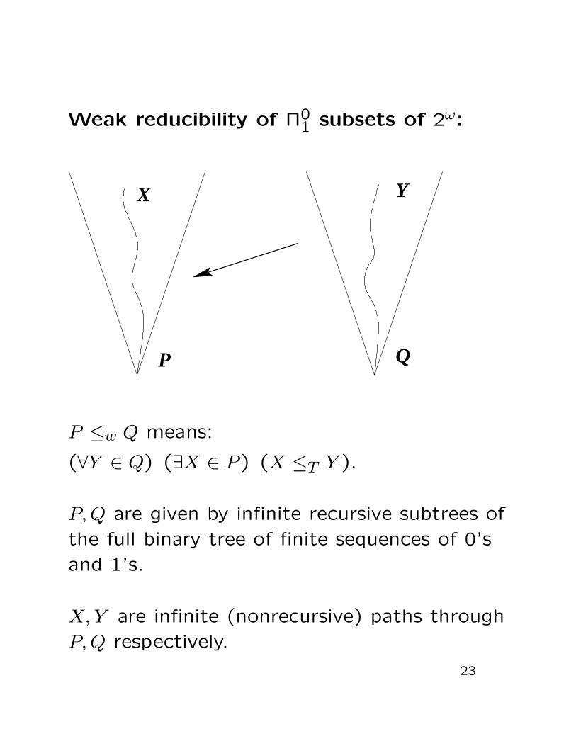
Weak reducibility of Π01 subsets of 2ω:
X Y
QP
P ≤w Q means:
(∀Y ∈ Q) (∃X ∈ P) (X ≤T Y ).
P, Q are given by infinite recursive subtrees of
the full binary tree of finite sequences of 0’s
and 1’s.
X, Y are infinite (nonrecursive) paths through
P, Q respectively.
23

Embedding RT into Pw:
Let RT be the upper semilattice of recursively
enumerable Turing degrees.
Theorem (Simpson 2002):
There is a natural embedding φ : RT → Pw.
The embedding φ is given by
φ : degT (A) 7→ degw(PA ∪ {A}).
Note: PA∪ {A} is not a Π01 set. However, it is
of the same weak degree as a Π01 set. This is
a non-obvious fact.
The embedding φ is one-to-one and preserves
≤, l.u.b., and the top and bottom elements.
The one-to-oneness is not obvious.
Convention:
We identify RT with its image in Pw under φ.
In particular, we identify 0′, 0 ∈ RT with the
top and bottom elements of Pw.
24

A picture of the lattice Pw:
r. e.Turingdegrees
the
0’ = PA����
���
���
0RT is embedded in Pw. 0′ and 0 are the topand bottom elements of both RT and Pw.
25

Specific, natural degrees in Pw:
A fundamental open problem concerning the
recursively enumerable Turing degrees is to
find a specific, natural example of such a
degree, other than 0 and 0′.
In the Pw context, we have discovered many
specific, natural degrees which are > 0 and
< 0′.
The specific, natural degrees in Pw which we
have discovered are related to foundationally
interesting topics:
• effective randomness,
• diagonal nonrecursiveness,
• reverse mathematics,
• subrecursive hierarchies,
• computational complexity.
26

r. e.Turingdegrees
the
d
inf (r ,0’)
r1
2
dREC
���
���
����
����
����
����
����
0’ = PA
0
Note. Except for 0′ and 0, the r.e. Turing
degrees are incomparable with all of these
specific, natural degrees in Pw.
27

Some specific, natural degrees in Pw.
rn = the weak degree of the set of n-randomreals.
d = the weak degree of the set of diagonallynonrecursive functions.
dREC = the weak degree of the set ofdiagonally nonrecursive functions which arerecursively bounded.
Theorem(Simpson 2002, Ambos-Spies et al 2004)
In Pw we have
0 < d < dREC < r1 < inf(r2, 0′) < 0′.
Theorem (Simpson 2002).
1. r1 is the maximum weak degree of a Π01
subset of 2ω which is of positive measure.
2. inf(r2, 0′) is the maximum weak degree ofa Π0
1 subset of 2ω whose Turing upwardclosure is of positive measure.
28

Another specific, natural degree in Pw is
provided by the work of Kjos-Hanssen and
Binns/Kjos-Hanssen/Miller/Solomon on
almost everywhere domination.
Definition. Let m = degw(AED) where
AED = {B | B is almost everywhere
dominating}.
It can be shown that inf(m, 0′) belongs to Pw.
Again, this is not obvious, because AED ∪ PA
is not Π01.
Interestingly, inf(m, 0′) lies below some
recursively enumerable Turing degrees which
are strictly below 0′. This is in contrast to
the behavior of r1, inf(r2, 0′), d, and dREC.
29

inf (m,0’)
degrees
the
d
inf (r ,0’)
r1
2
dREC
r. e.Turing
0’ = PA����
����
����
����
����
��������
0���
���
Note how the behavior of inf(m, 0′) contrasts
with that of inf(r2, 0′), r1, dREC, and d.
Questions????
30
Some additional examples ?
It seems reasonable to think that additional
examples of specific, natural degrees in Pw
could be obtained by replacing measure by
Hausdorff dimension.
For rational s with 0 ≤ s ≤ 1, let
Qs = {X ∈ 2ω | dim(X) = s}. Here dim
denotes effective Hausdorff dimension as
defined by Jack Lutz.
The Qs’s are uniformly Σ03, so by the
Embedding Lemma we have
qs = degw(Qs) ∈ Pw and
q>s = inft>s qt ∈ Pw. By “dilution” we have
qs ≤ qt ≤ r1 for all s < t.
Question. What other relationships hold
among the qs’s?
31

Question. What relationships hold among
the qs’s?
Conceivably qs < qt < r1 for all s < t ≤ 1. At
the other extreme, it is possible that qs = r1for all s > 0.
This is essentially just Reimann’s “dimension
extraction problem”. The problem is, does
dim(X) > 0 imply existence of Y ≤T X such
that Y is random? Does 0 < dim(X) < 1
imply existence of Y ≤T X such that
dim(Y ) > dim(X)?
Question. What relationships hold among
the qs’s and other specific, natural degrees in
Pw such as r1, dREC, d, etc.?
Question. Can we find specific, natural
degrees in Pw analogous to inf(m, 0′),
replacing positive measure domination by
positive Hausdorff dimension domination,
positive effective Hausdorff dimension
domination, etc.?
32

Smallness properties of Π01 subsets of 2ω.
There are many “smallness properties” of Π01
sets P ⊆ 2ω which insure that the weakdegree of P is > 0 and < 0′. Here is oneresult of this type.
Definition.
A Π01 set P ⊆ 2ω is said to be thin if,
for all Π01 sets Q ⊆ P , P \ Q is Π0
1.
Thin perfect Π01 subsets of 2ω have been
constructed by means of priority arguments.Much is known about them. For example,any two such sets are automorphic in thelattice of Π0
1 subsets of 2ω under inclusion.
See Martin/Pour-El 1970,Downey/Jockusch/Stob 1990, 1996,Cholak et al 2001.
Theorem (Simpson 2002).
Let p be the weak degree of a Π01 set P ⊆ 2ω
which is thin and perfect. Then p isincomparable with r1. Hence 0 < p < 0′.
33

Relationship to measure and dimension.
Theorem (Simpson 2002). If P ⊆ 2ω is thin
and perfect, then P is of measure 0.
Theorem (Binns 2006). If P ⊆ 2ω is thin and
perfect, then P is of Hausdorff dimension 0.
Note (Hitchcock 2000). For any Π01 set
P ⊆ 2ω, the effective Hausdorff dimension of
P is equal to the Hausdorff dimension of P .
Question (Simpson 2002). Does there exist
a thin perfect Π01 set P ⊆ 2ω such that the
Turing upward closure of P is of measure
> 0?
Note. This is equivalent to asking whether
the weak degree of such a set can be
≤ inf(r2, 0′).
Note (Reimann). By a theorem in Reimann’s
thesis, all Turing cones are of Hausdorff
dimension 1.
34
Some additional “smallness properties”:
Let P be a Π01 subset of 2ω.
Definition. P is small if there is no recursive
function f such that for all n there exist n
members of P which differ at level f(n) in the
binary tree. (Binns 2003)
Example. Let A ⊆ ω be hypersimple, and let
A = B1 ∪ B2 where B1, B2 are r.e. Then
P = {X ∈ 2ω | X separates B1, B2} is small.
Definition. P is h-small if there is no
recursive, canonically indexed sequence of
pairwise disjoint clopen sets Dn, n ∈ ω, such
that P ∩ Dn 6= ∅ for all n. (Simpson 2003)
For many of these smallness properties, there
are results and questions similar to the ones
which we formulated above for thin perfect
Π01 sets. One can ask about the measure and
dimension of P , and about the measure of
the Turing upward closure of P .
35

Additional references:
Stephen Binns, Small Π01 classes, Archive for
Mathematical Logic, 45, 2006, 393–410.
Stephen G. Simpson, Mass problems and randomness,Bulletin of Symbolic Logic, 11, 2005, 1–27.
Stephen G. Simpson, An extension of the recursivelyenumerable Turing degrees, 15 pages, Journal of the
London Mathematical Society, to appear
Stephen G. Simpson, Some fundamental issuesconcerning degrees of unsolvability, 18 pages, toappear in Computational Prospects of Infinity, editedby C.-T. Chong, Q. Feng, T. A. Slaman, W. H.Woodin, and Y. Yang, World Scientific, to appear.
Stephen G. Simpson, Almost everywhere dominationand superhighness, preprint, 28 pages, July 2006, inpreparation.
Some of my papers are available at
http://www.math.psu.edu/simpson/papers/.
Transparencies for my talks are available at
http://www.math.psu.edu/simpson/talks/.
THE END
36