HAL Id: hal-01305993https://hal.archives-ouvertes.fr/hal-01305993

Submitted on 22 Apr 2016

HAL is a multi-disciplinary open accessarchive for the deposit and dissemination of sci-entific research documents, whether they are pub-lished or not. The documents may come fromteaching and research institutions in France orabroad, or from public or private research centers.

L’archive ouverte pluridisciplinaire HAL, estdestinée au dépôt et à la diffusion de documentsscientifiques de niveau recherche, publiés ou non,émanant des établissements d’enseignement et derecherche français ou étrangers, des laboratoirespublics ou privés.

Review & Perspective for Distance Based Clustering ofVehicle Trajectories

Philippe Besse, Brendan Guillouet, Jean-Michel Loubes, François Royer

To cite this version:Philippe Besse, Brendan Guillouet, Jean-Michel Loubes, François Royer. Review & Perspective forDistance Based Clustering of Vehicle Trajectories. IEEE Transactions on Intelligent TransportationSystems, IEEE, 2016, 17 (11), pp.3306-3317. �10.1109/TITS.2016.2547641�. �hal-01305993�

1

Review & Perspective forDistance Based Clustering of Vehicle Trajectories

Philippe C. Besse, Brendan Guillouet, Jean-Michel Loubes, and Francois Royer,

Abstract—In this paper we tackle the issue of clusteringtrajectories of geolocalized observations based on distance be-tween trajectories. We first provide a comprehensive reviewof the different distances used in the literature to comparetrajectories. Then based on the limitations of these methods, weintroduce a new distance: Symmetrized Segment-Path Distance(SSPD). We compare this new distance to the others accordingto their corresponding clustering results obtained using boththe hierarchical clustering and affinity propagation methods. Wefinally present a python package : trajectory distance, whichcontains the methods for calculating the SSPD distance and theother distances reviewed in this paper.

Index Terms—Trajectory clustering

I. INTRODUCTION

ATRAJECTORY is a set of positional information for amoving object, ordered by time. This kind of multidi-

mensional data is prevalent in many fields and applications,for example, for understanding migration patterns throughstudying trajectories of animals, predicting meteorology withhurricane data, improving athletes performance, etc. Our studyconcentrates on vehicle trajectories within a road network. Thegrowing use of GPS receivers and WIFI-embedded mobiledevices equipped with hardware for storing data enables thecollection of an enormous amount of data that can be used toextract relevant information in order, for instance, to find theoptimal path to go from point A to point B, detect abnormalbehavior, optimize the traffic flow in a city, predict the nextlocation or final destination of a moving object etc. Thisaims actually to build from the data the different features thatcharacterize the different daily movement of the vehicles onthe road network. For this, we consider clustering methodsfor trajectories. Clustering techniques aim to regroup similartrajectories together into groups that are different from oneanother. The complexity of trajectory makes this a challengingtask as objects can move along many different paths in a givenarea, moreover the road network of a highway does not havethe same complexity as that of a city, and finally the roadnetwork in a city differs between the suburbs and downtown.In addition, the speed of an object varies between regions, andbetween paths taken within a single region. Even within thesame path the speed depends on exogenous variables such asthe time of day, or whether it is a weekday or the weekend.

Several methods can be used to cluster trajectories. We willfocus on distance based trajectory clustering but other spe-cific methodologies have been investigated. Dealing with thefunctional properties of trajectories considered as continuous

function of time Gaffney (2009, [1]), Vasquez et al. (2004[2]),Hu et al. (2006[3]) successfully apply trajectory clusteringmethods on video-stream trajectories. Gariel et al. [4] alsouse the continuous definition of trajectory to re-sample thetrajectories and obtain time series of equal length. A principalcomponents analysis is then applied on these new trajectoriesto obtain principal components and finally cluster them. Thismethod is applied to airplane routes. All these methods takeinto account both the spatial and the temporal aspect of thetrajectory, they are not adapted to the vehicle trajectoriesconstrained to a road network whose time progression isvery irregular. Rinzivillo et al. (2008,[5]) and Kim et al.[6])propose density-based methods. Both require the definitionof a density parameter and a minimum cluster size whichimplies an extensive knowledge of the studied area or a precisequestion to obtain good results. Hence, these methods are hardto automatically adapt from one dataset to another. FinallyLee et al. (2007,[7]) and Wu et al. (2014[8]) propose to useclustering methods on trajectory line segments to enable thedetection of important areas of flow, though this does notconsider the trajectory as a whole path. Our main objectivehere is to detect the main path and traffic flow which can laterbe used to study the different behaviors along these paths.

In this context, the goal of this work is to construct, in adata driven way, a collection of trajectories that model thebehaviors of car drivers. These models are learned from adata set of car locations. In this work we focus on clusteringtrajectories having similar paths. This clustering is based onthe comparison between trajectory objects, and as such a newdefinition of distance between the studied trajectory objects isrequired.

A large amount of work has been done to give new defini-tions of trajectory distance. Tiakas et al.(2009[9]) , Rossi etal. (2012[10]), Han et al.(2015[11]) or Hwang et al.(2005[12])propose road network based distances. They assume that thetrajectories studied are perfectly mapped on the road network.However, this task is strongly dependent on the precision ofthe GPS device. When the time interval between two GPSlocations is significant, several paths on the graph are possiblebetween locations, especially when the network is dense.Moreover it requires the knowledge of the road network. Here,we focus on entirely data driven methods without any a prioriinformation. Several methods have been used to cluster data setof trajectories. Clustering methods using Euclidean distancelead to inaccurate results mainly because trajectories havedifferent lengths. Hence, several methods based on warpingdistance have been defined , Berndt (1994[13]), Vlachos etal. (2002[14]), Chen et al. (2004[15]), and Chen et al. (2005

2

[16]). These methods reorganize the time index of trajectoriesto obtain a perfect match between them. Another approach isto focus on the geometry of the trajectories, in particular theirshape. Shape distances like Hausdorff and Frechet distancescan be adapted to trajectories but fail to compare them asa single entity. Lin et al. (2005[17]) proposed a methodbased exclusively on the shape of the trajectory but at highcomputational cost.

In section II the papers definitions, notations and problemstatement are introduced. In section III several distances ontrajectory are studied and compared. A new distance willbe presented in section IV: the Symetrized Segment-PathDistance (SSPD). SSPD is a shape-based distance that does nottake into account the time index of the trajectory. It comparestrajectories as a whole, and is less affected by incidentalvariation between trajectories. It also takes into account thetotal length, the variation and the physical distance betweentwo trajectories. For all these different distances, we obtaindifferent clusterings. So we can compare the distance on theseresults. The choice of clustering used is detailed section V. TheSSPD and the other studied distances were implemented in apython package, trajectory distance available on github. Thepresentation of this package and the experimental evaluationof these distances with the chosen clustering techniques onsome trajectory sets are analyzed in section VI.

II. MODEL FOR TRAJECTORY CLUSTERING

A. Trajectory

A continuous trajectory is a function which gives thelocation of a moving object as a continuous function of time.In our case we will only consider discrete trajectories definedhere after.

Definition 1. A trajectory T is defined asT : ((p1, t1), . . . , (pn, tn)),where pk ∈ R2, tk ∈ R ∀k ∈ [1 . . . n], ∀n ∈ N and n is thelength of the trajectory T .

The exact locations between time ti and ti+1 are unknown.When these locations are required, a piece wise linear repre-sentation is used between each successive location pi and pi+1

resulting in a line segment si between these two points. Thisnew representation is called a piece wise linear trajectory. Inthis representation, no assumption is made about time indexingof segment si.

Definition 2. A piece wise linear trajectory is defined as Tpl: ((s1), . . . , (sn−1)) , where sk ∈ R4 and npl is the length ofthe trajectory.

The length of the trajectory npl is the sum of the lengths ofall segments that compose it : npl =

∑i∈[1...n−1] ‖pipi+1‖2.

The notation used in this paper are summarized in Table I.

B. Distance

There are many ways to define how close two objects arefrom one another. Beyond the notion of mathematical distance,many functions can be used to qualify this dissimilarity. Theterminology used in literature to define them is not completely

standardized. Therefore we will use the definition establishedin Deza et al. (2009[18]) as a reference.

Definition 3. Let T be a set of trajectories. A function d :T ×T 7→ R is called a dissimilarity on T if for all T 1, T 2 ∈T :

• d(T 1, T 2) ≥ 0• d(T 1, T 2) = d(T 2, T 1)• d(T 1, T 1) = 0

If all of these conditions are satisfied and d(T 1, T 2) =0 =⇒ T 1 = T 2 d is considered to be a symmetric. Ifthe triangle inequality is also satisfied, d is called a metric.These notations are summarized in Table II.

X indicates the required properties for each distances, while∗ indicates properties that are automatically satisfied (by thepresence of the other required properties for the metric).

C. Desired properties of clustering and distances

Our aim is to regroup trajectories sharing similar behaviour.We want that trajectories in the same cluster, take similarpaths. Hence our goal is to define a clustering method thatwill regroup trajectories• with similar shape and length• which are physically close to each other• which are similar as a whole with more than just similar

sub-parts• all of these properties should be considered without

regard to their time indexingMoreover we want to design a very general procedure which

is able to treat all trajectories data, without prior knowledge ofthe particular geographical location where they are collected.To obtain such clustering, the goal of this work is to finda distance that respects such properties and to succeed inextracting these features. Actually, the desired distance shouldhave the following properties,• it compares trajectories as a whole• the compared trajectories can be of different lengths,• the time indexing can be very different from one trajec-

tory to another• the trajectories can have similar shapes but can be phys-

ically far from each other and vice versa

TABLE I: Notation

T The set of trajectories

T i The ith trajectory of set T

T ipl The piece wise linear representation of T i

ni Length of trajectory T i

nipl Length of the T i

pl

pik The kth location of T i

pipl The set of continuous points that compose T ipl

sik The line segment between pij and pik+1

tik The time index of location pik

‖pkpl‖2 The Euclidean distance between pk and pl

3

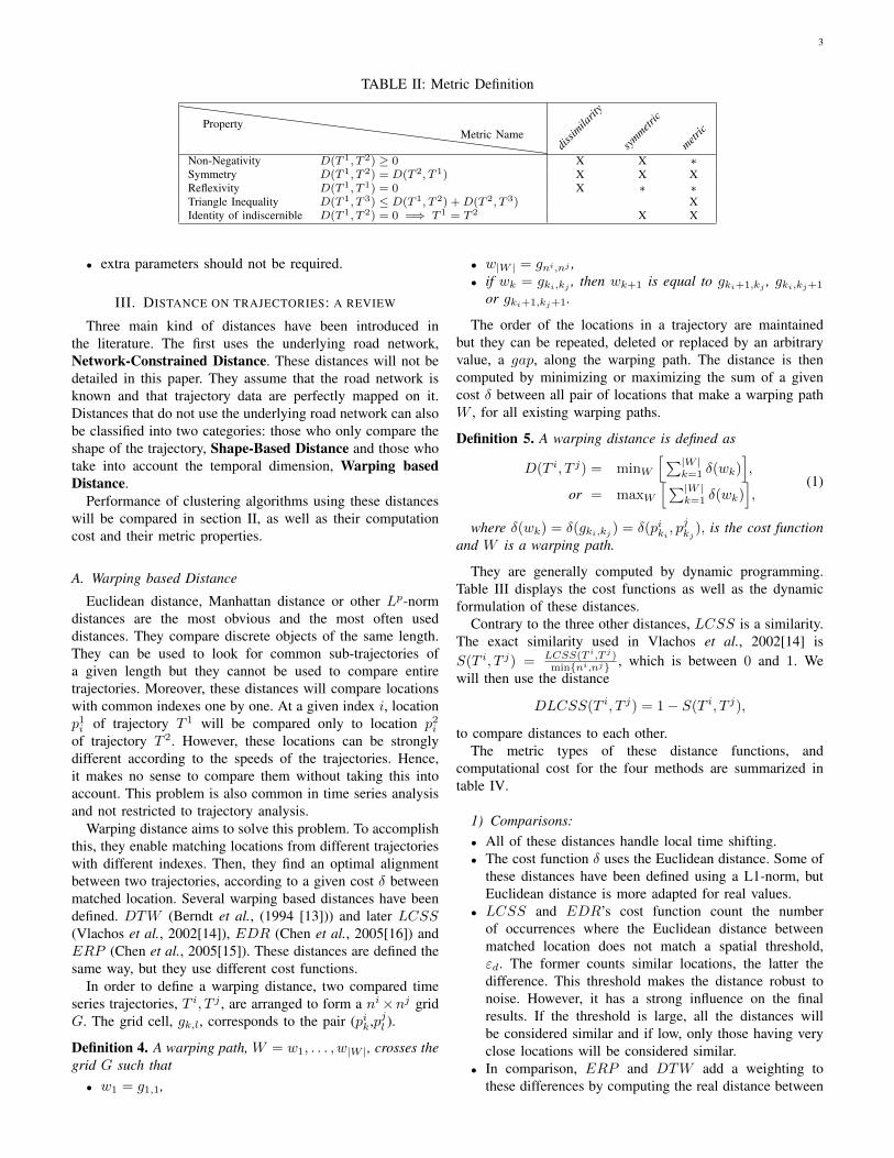
TABLE II: Metric Definition

PropertyMetric Name

dissim

ilarit

y

symmetr

ic

metric

Non-Negativity D(T 1, T 2) ≥ 0 X X ∗Symmetry D(T 1, T 2) = D(T 2, T 1) X X XReflexivity D(T 1, T 1) = 0 X ∗ ∗Triangle Inequality D(T 1, T 3) ≤ D(T 1, T 2) +D(T 2, T 3) XIdentity of indiscernible D(T 1, T 2) = 0 =⇒ T 1 = T 2 X X

• extra parameters should not be required.

III. DISTANCE ON TRAJECTORIES: A REVIEW

Three main kind of distances have been introduced inthe literature. The first uses the underlying road network,Network-Constrained Distance. These distances will not bedetailed in this paper. They assume that the road network isknown and that trajectory data are perfectly mapped on it.Distances that do not use the underlying road network can alsobe classified into two categories: those who only compare theshape of the trajectory, Shape-Based Distance and those whotake into account the temporal dimension, Warping basedDistance.

Performance of clustering algorithms using these distanceswill be compared in section II, as well as their computationcost and their metric properties.

A. Warping based Distance

Euclidean distance, Manhattan distance or other Lp-normdistances are the most obvious and the most often useddistances. They compare discrete objects of the same length.They can be used to look for common sub-trajectories ofa given length but they cannot be used to compare entiretrajectories. Moreover, these distances will compare locationswith common indexes one by one. At a given index i, locationp1i of trajectory T 1 will be compared only to location p2iof trajectory T 2. However, these locations can be stronglydifferent according to the speeds of the trajectories. Hence,it makes no sense to compare them without taking this intoaccount. This problem is also common in time series analysisand not restricted to trajectory analysis.

Warping distance aims to solve this problem. To accomplishthis, they enable matching locations from different trajectorieswith different indexes. Then, they find an optimal alignmentbetween two trajectories, according to a given cost δ betweenmatched location. Several warping based distances have beendefined. DTW (Berndt et al., (1994 [13])) and later LCSS(Vlachos et al., 2002[14]), EDR (Chen et al., 2005[16]) andERP (Chen et al., 2005[15]). These distances are defined thesame way, but they use different cost functions.

In order to define a warping distance, two compared timeseries trajectories, T i, T j , are arranged to form a ni×nj gridG. The grid cell, gk,l, corresponds to the pair (pik,pjl ).

Definition 4. A warping path, W = w1, . . . , w|W |, crosses thegrid G such that• w1 = g1,1,

• w|W | = gni,nj ,• if wk = gki,kj , then wk+1 is equal to gki+1,kj , gki,kj+1

or gki+1,kj+1.

The order of the locations in a trajectory are maintainedbut they can be repeated, deleted or replaced by an arbitraryvalue, a gap, along the warping path. The distance is thencomputed by minimizing or maximizing the sum of a givencost δ between all pair of locations that make a warping pathW , for all existing warping paths.

Definition 5. A warping distance is defined as

D(T i, T j) = minW

[∑|W |k=1 δ(wk)

],

or = maxW

[∑|W |k=1 δ(wk)

],

(1)

where δ(wk) = δ(gki,kj ) = δ(piki , pjkj), is the cost function

and W is a warping path.

They are generally computed by dynamic programming.Table III displays the cost functions as well as the dynamicformulation of these distances.

Contrary to the three other distances, LCSS is a similarity.The exact similarity used in Vlachos et al., 2002[14] isS(T i, T j) = LCSS(T i,T j)

min{ni,nj} , which is between 0 and 1. Wewill then use the distance

DLCSS(T i, T j) = 1− S(T i, T j),

to compare distances to each other.The metric types of these distance functions, and

computational cost for the four methods are summarized intable IV.

1) Comparisons:• All of these distances handle local time shifting.• The cost function δ uses the Euclidean distance. Some of

these distances have been defined using a L1-norm, butEuclidean distance is more adapted for real values.

• LCSS and EDR’s cost function count the numberof occurrences where the Euclidean distance betweenmatched location does not match a spatial threshold,εd. The former counts similar locations, the latter thedifference. This threshold makes the distance robust tonoise. However, it has a strong influence on the finalresults. If the threshold is large, all the distances willbe considered similar and if low, only those having veryclose locations will be considered similar.

• In comparison, ERP and DTW add a weighting tothese differences by computing the real distance between

4

TABLE III: Re-Indexing based distance definitionCost function Distance

δNAME(p1, p2) = NAME(T i, T j) =

DT

W‖p1p2‖2 =

0 if ni = nj = 0∞ if ni = 0 or nj = 0

δDTW (pi1, pj1)+

min

{ DTW (rest(T i), rest(T j)),DTW (rest(T i), T j)),DTW (T i, rest(T j)

}otherwise

NA

ME L

CSS

1 if ‖p1p2‖2 < εd0 if p1 or p2 is a gap0 otherwise

=

0 if ni = 0 or nj = 0

LCSS(rest(T i), rest(T j)) + δLCSS(pi1, p

j1) if δLCSS(p

i1, p

j1) = 1

max

{LCSS(rest(T i), T j)) + δLCSS(p

i1, gap),

LCSS(T i, rest(T j)) + δLCSS(gap, pj1)

}otherwise

ED

R

0 if ‖p1p2‖2 < εd1 if p1 or p2 is a gap1 otherwise

=

ni if nj = 0nj if ni = 0

EDR(rest(T i), rest(T j)) if δEDR(pi1, pj1) = 0

min

{ EDR(rest(T i), rest(T j)) + δEDR(pi1, pj1),

EDR(rest(T i), T j)) + δEDR(pi1, gap),

EDR(T i, rest(T j) + δEDR(gap, pj1)

}otherwise

ER

P

‖p1p2‖2 if p1, p2 are not gaps‖p1g‖2 if p2 is a gap‖gp2‖2 if p1 is a gap

=

∑ni

k=1 ‖pikg‖2 if nj = 0∑nj

l=1 ‖pjl g‖2 if ni = 0

min

{ ERP (rest(T i), rest(T j)) + δERP (pi1, pj1),

ERP (rest(T i), T j)) + δERP (pi1, gap),

ERP (T i, rest(T j) + δERP (gap, pj1)

}otherwise

TABLE IV: Re-Indexing based distance properties

Name Metric Types ComputationCost

DTW symmetric O(n2)LCSS distance O(n2)EDR symmetric O(n2)ERP metric O(n2)

the locations. In this sense they can be viewed as moreaccurate.

• ERP is the only distance which is a metric regardlessof the Lp norm used, yet it works better for normalizedsequences, especially for defining the gap value g. It doesnot apply for vehicle trajectories.

• In addition, these distances may include a time threshold,εt. Thus, two locations will not be compared if the differ-ence between their time indexing is too large. However, itis very hard to estimate the value of this threshold whencomparing trajectories due to the presence of noise.

2) Pros and Cons: The main advantage of these distances isthat they enable comparison of sequences of different lengths.

The two main limitations of warping based distance are thefollowing• Warping methods are based on one-to-one comparison

between sequences. Hence, it often requires the choiceof a particular series that will be used as a reference,onto which all other sequences will be mapped. Theindex of two sequences being compared should be wellbalanced in order to best capture the variability, forinstance, in order to detect if there were accelerationsand decelerations during the measurement of the timeseries. Hence the choice of the reference sequence is veryimportant.

• The performance of the usual methods based on warpingtechniques is hampered by the large amount of noiseinherent to road traffic data, which is not the case whenexamining time series.

Instead of correcting the time index, the solution is to usedistances that have the effect of time removed.

B. Shape-Based Distance

These distances try to catch geometric features of thetrajectories, in particular, their shape. Among Shape-BasedDistances, the Hausdorff distance (Hausdorff, 1914 [19]),and the Frechet distance (Frechet, 1906[20]) are likely themost well known.

1) Hausdorff: The Hausdorff distance is a metric. It mea-sures the distance between two sets of metric spaces. Infor-mally, for every point of set 1, the infimum distance from thispoint to any other point in set 2 is computed. The supremumof all these distances defines the Hausdorff distance.

Definition 6. The Hausdorff distance between two sets ofmetric spaces is defined as

Haus(X,Y ) = max{supx∈X

infy∈Y‖xy‖2, sup

y∈Yinfx∈X‖xy‖2}.

This distance is complicated and resource intensive tocompute when applied to most existing sets. But in the case ofpolygonal curves like trajectories, some simplification can bemade due to the monotonic properties of a segment. Distancefrom a point p to a segment s is defined as follows.

Definition 7. Point− to− Segment distance.

Dps(p1i1 , s

2i2) =

{‖p1i1p

1proji1

‖2 if p1proji1∈ s2i2 ,

min(‖p1i1p2i2‖2, ‖p

1i1p

2i2+1‖2) otherwise.

Where p1proji1is the orthogonal projection of p1i1 on the

segment s2i2 .

Hence, the Hausdorff distance between two line segmentsis

DHaussdorf (s1i1, s2i2) = max{ supp∈s1i1 Dps(p, s

2i2),

supp∈s2i2Dps(p, s

1i1)}

= max{ Dps(p1i1, s2i2), Dps(p

1i1+1, s

2i2),

Dps(p2i2, s1i1), Dps(p

2i2+1, s

1i1)}.

Indeed, a segment is monotonic. As seen in Fig. 1, thesupremum of the Point− to− Segments distance from any

5

Fig. 1: Supremum of Point − to − Segment distance frompoint of segment s11 to segment s21.

point of a segment s1i1 to a segment s2i2 occurs at one of the endpoints of the segment s1i1 . The Hausdorff distance between twotrajectories can then be computed with the following formula.

Definition 8. Hausdorff distance between two discrete trajec-tories.

DHaussdorf (T1, T 2) = max

{max i1∈[1...n1]

j2∈[1...n2−1]

{Dps(p1i1, s

2j2},

maxj1∈[1...n1−1]

i2∈[1...n2]

{Dps(p2i2, s

1j1}

}.

The Hausdorff distance can then be computed in a O(n2)computational time.

2) Frechet and discrete Frechet : The Frechet distancemeasures similarity between curves. It is often known as the”walking-dog distance”. Imagine a dog and its owner walkingon two separate paths without backtracking from one endpointto one other. The Frechet distance is the minimum lengthof leash required to connect a dog and its owner. While theHausdorff distance takes distance between arbitrary points, theFrechet metric takes the form of the two curves into account.

Definition 9. The Frechet distance between two curves isdefined as

DFrechet(A,B) = infα,β∈X

maxt∈[0,1]

{‖A(α(t)

), B(β(t)

)‖2}.

Similar to the Hausdorff distance, the Frechet distance isa metric. It is also resource intensive. Alt et al. (1995[21])developed an algorithm measuring the exact Frechet distancefor polygonal curves based on the free space definition.

Definition 10. The free space Fε(T 1, T 2) between two trajec-tories is the set of all pairs of points whose distance is at mostε.

Fε(T1, T 2) := {(p1, p2) ∈ (T 1, T 2)}|‖p1, p2‖2 ≤ ε}.

The Frechet distance between two trajectories T 1 and T 2

is the minimum value of ε for which a curve exists within thecorresponding Fε from (p10, p

20) to (p1n1 , p2n2) with the property

of being monotone existing in both trajectories. Computing theFrechet distance means finding the minimum value of ε. Byexploiting the monotonic property of the segments and thedefinition of free space, this task can be accomplished moreefficiently.

Indeed, the Frechet distance between segments is equal tothe Hausdorff distance between segments, i.e.

DFrechet(s1i1, s2i2) = max{ Dps(p

1i1, s2i2),

Dps(p1i1+1, s

2i2),

Dps(p2i2, s1i1),

Dps(p2i2+1, s

1i1)}

= εi1,i2 .

To compute the Frechet distance between trajectories T 1

and T 2 , we need only look among the set E of Frechetdistances between all pairs of segments of T 1 and T 2.E = {εi1,i2 for (i1, i2) ∈ ([1 . . . n1 − 1] × [1 . . . n2 − 1])}.This simplification enables us to compute the Frechet distancebetween trajectories T 1 and T 2 in O(n2log(n2)). We highlightthat this computational cost is higher than all the othercalculation methods of the studied distances.

Eiter et al. (1994[22]) describes an approximation of thisdistance for polygonal curves called the discrete Frechetdistance. This distance is close to the definition of the warpingbased distance.

Definition 11. The discrete Frechet distance is defined as

DFrechetDiscr((T 1, T 2) = min

W{ maxk∈[1...|W |]

‖wk‖2}.

with W being the warping path defined in definition 5. Thediscrete Frechet distance can be computed in O(n2) time.

This distance is bounded as follows.

Theorem 1. For any trajectories T i and T j [22]

DFrechet(Ti, T j) ≤ DFrechetDiscr

((T i, T j) ≤ DFrechet(Ti, T j)+ε

Where, ε = max{ maxk∈[1...ni−1]

{‖pikpik+1‖2}, maxl∈[1...nj−1]

{‖pjl pjl+1‖2}}.

3) One Way Distance: Lin et al. 2005[17] defines the One-Way-Distance, OWD, from a trajectory T i to another trajectoryT j as the integral of the distance from points of T ipl totrajectory T jpl divided by the length of T ipl

Definition 12. The OWD distance is defined as

DOWD(Ti, T j) =

1

nipl

∫pi∈T i

pl

Dpoint(piT j)dpi,

where Dpoint(p, T ) is the distance from the point p to thetrajectory T so that

6

TABLE V: Shape based distance properties

Name Metric Types ComputationCost

Hausdorff metric O(n2)Frechet metric O(n2log(n2))

discrete Frechet symmetric O(n2)OWD symmetric O(n2log(n))

OWDgrid symmetric O(mn)

Dpoint(p, T ) = minq∈Tpl

‖pq‖2.

The OWD distance is not symmetric, butDSOWD(T

i, T j) = (DOWD(Ti, T j) + DOWD(T

j , T i))/2is. This distance is a symmetric because it does not satisfythe triangle inequality.

Lin et al.[17], have defined two algorithms to compute theOWD in case of piecewise linear trajectories.• The first consists of finding the parametrized OWD

function DOWD(sik, T

j) from a segment sik of T ipl toall segments sj of T jpl and for all segments of T ipl

DOWD(Ti, T j) =

1

nipl

ni−1∑k=1

DOWD(sik, T

j).‖pikpik+1‖,

with a complexity of O(n2log(n)).• The second uses a grid representation of the trajectory.

As we see in Fig. 2, the space is discrete Trajectories aredefined as the succession of grids they have crossed.

Definition 13. A grid representation trajectory is definedas

Tgrid := (g0, . . . , gngrid),

where gn are cells of the discrete space.

Fig. 2: Grid representation of a segment

This representation simplifies the computation and re-duces the complexity to O(nm) where m is the numberof local min points. Local min points of a grid cell g arethe grids with distances to g shorter than those of theirneighbors’ grid cell.

Table V displays the metric types and the computationalcost of these distances.

4) Pros and Cons:

• Frechet and Hausdorff distances are both metrics, mean-ing they satisfy triangular inequality. With clusteringalgorithms like dbscan or K-medoid this is a necessaryproperty of the distance used if we want the clusteringalgorithm to be efficient. They have been widely used inmany domains where shape comparison is needed. Butthey can fail to compare trajectories as a whole. Indeedboth Frechet and Hausdorff distance return a maximumdistance between two objects at given points within thetwo objects. As we can see in Fig. 3, despite the factthat the trajectories T 1 and T 2 are well separated atthe maximum value of x, they are clearly more similarto each other than to T 3. But with a Hausdorff calcu-lated distance, there are no strong differences betweenDHaussdorf (T

1, T 2) = 3.26, DHaussdorf (T1, T 3) =

3.02 and DHaussdorf (T2, T 3) = 3.5. With Frechet,

DFrechet(T1, T 2) = 6 is even bigger than both

DFrechet(T1, T 3) = 4.19 and DFrechet(T

2, T 3) = 4.17.

Fig. 3: Frechet And Hausdorff Computation between threetrajectories

• The Discrete Frechet distance requires considerably lesscomputing time compared to the Frechet distance. ButDiscrete Frechet is not a metric. Moreover, due to itssimilarity with the warping distance it shares the sameinconveniences.

• The distance present in Lin et al. (2005[17]) is by farthe one that best meets our requirements. It comparestrajectories as a whole, taking into account their shapesand their physical distances, the required features forour distance. However, its complexity makes it com-putationally slow. The algorithm for grid representationis faster. Its computational time is O(mn). Yet it doesnot take into account the computation time required formatching the trajectory to the grid. Moreover, the size ofthe grid chosen strongly influences the final result andmakes it imprecise. Furthermore, the distance gives thesame ”weight” to all points defining the trajectory: pointsdirectly issued from the GPS location, and points whichcompose the piece wise linear representation. The greaterthe length of the segment s is, the stronger its influenceon the trajectory is. The more separated the endpointsof a segment s are, the less confident the interpolationbetween them is.

In the following section, a new distance will be establishedinspired from both the OWD and the Hausdorff distances.

7

IV. A NEW DISTANCE : SYMMETRIZED SEGMENT-PATHDISTANCE (SSPD)

In this section, we define a new shape based distance, theSymmetrized Segment-Path Distance, and we compare it toother shape based distances. We propose SSPD in order tofulfill the desired properties defined in section II-C.

Like the Hausdorff distance (Definition 8), the definitionof SSPD is based on the Point − to − Segment distance(Definition 7). From this definition, we define the Point−to−Trajectory distance, Dpt, from a point p to a trajectory T likethe minimum of distances between this point and all segmentss that compose T (Figure 4). The Segment-Path distance fromtrajectory T 1 to trajectory T 2 is the mean of all distances frompoints composing T 1 to the trajectory T 2 (Figure 5).

Definition 14. SPD distance is defined as

DSPD(T1, T 2) =

1

n1

n1∑i1=1

Dpt(p1i1 , T

2).

where, Dpt(p1i1, T 2) = mini2∈[0,...,n2−1]Dps(p

1i1, s2i2).

Fig. 4: Distance from point p21 to trajectory T 1

Proposition 1. If the points that compose the trajectory T 1

lie in the set of points p2pl that compose the piece wise linearrepresentation, T 2

pl, of trajectory T 2, then DSPD(T1, T 2) = 0.

Proof. If the points that compose the trajectory T 1 lie inthe set p2pl that compose the piece wise linear representation,T 2pl, of trajectory T 2, all points of T 1 lie within one of the

segments, that compose T 2pl. By definition Dps(p

1i1, s2i2) = 0

Fig. 5: SPD Distance from trajectory T 1 to trajectory T 2

∀p1i1 ∈ T 1, s2i1 ∈ T 2pl. It follows that Dpt(p

1i1, T 2) = 0

∀p1i1 ∈ T1 and finally DSPD(T

1, T 2) = 0

This distance is not symmetric. If T 1 is a very small sub-trajectory of T 2, DSPD(T

1, T 2) = 0, DSPD(T2, T 1) can

be very large. By taking the mean of these distances, the”Symmetrized Segment-Path Distance”, SSPD, is definedand is symmetric.

Definition 15. Symmetrized Segment-Path Distance

DSSPD(T1, T 2) =

DSPD(T1, T 2) +DSPD(T

2, T 1)

2.

In definitions 14 and 15, distances SPD and SSPD arecomputed by taking the mean of the Point-to-Trajectory dis-tance and the SPD distance. If the maximum is used insteadof the mean, one recovers the Hausdorff function betweentwo trajectories. Computing only one distance between twolocations makes it very sensitive to noise. Yet our methodcomputes the mean of such quantities which makes it less so.For example, for the trajectories in Fig. 3, the SSPD distancebetween T 1 and T 2 is smaller than the distance between T 1

and T 3 or T 2 and T 3 (D(T 1, T 2) = 0.58, D(T 1, T 3) =1.5, D(T 2, T 3) = 2.03).

Proposition 2. SSDP is a symmetric.

Proof. SSDP is a sum of Euclidean distances. By definitionSSDP is greater or equal to 0. By definition 15, SSDP is sym-metric. Finally theorem 1 states that, if DSDP (T

1, T 2) = 0,T 1 is a sub trajectory of T 2. Therefore if DSSDP (T

1, T 2) =0, both DSDP (T

1, T 2) = 0 and DSDP (T1, T 2) = 0, and

T 1 = T 2. SSDP is then a symmetric.

8

SSDP is quite similar to OWD but its definition resolvesmost of the problems of OWD regarding the desired propertiesdefined in II-C• The points coming from the interpolation of two observed

locations of a trajectory are less trustworthy that the realobservations. Hence, it is natural to give more weight tothe observed points.

• SSPD distance does not require any additional parameterssuch as a threshold or a grid to be computed.

• Its computation cost is O(n2). It only depends on thenumber of locations.

V. CLUSTERING

To evaluate these different distances, we will study differentclustering methods obtained with the same algorithm but withdistances computed using all previous distances. The differentselected clustering methods and the quality of cluster criterionare examined in this section.

A. Methods

The choice of the clustering method is restricted by thecharacteristics of the trajectory object. Indeed, trajectories havedifferent lengths which complicates an easy definition of amean trajectory object. The k-means method cannot be usedon our trajectory set, nor spectral clustering method. k-medoidcan be used but an efficient algorithm, like partitioning aroundmedoids, or dbscan method, require a valid metrics. Indeed,these algorithms are based on nearest neighbor and require thedistance used to be known in order to satisfy the triangularinequality. Most of the studied distances, SSPD, LCSS, DTW,are not metrics. In this way, dbscan or partitioning aroundmedoids algorithms will not be used. Moreover, dbscan de-pends on two extra parameters that are hard to estimate inthis case.

To perform the clustering of the trajectories, we will focuson two methodologies : hierarchical cluster analysis (HCA)and affinity propagation (AP). As a matter of fact, HCAand AP can use distance/similarity which does not satisfythe triangle inequality. We point out that the choice of theclustering method is restricted to the trajectory object we dealwith. Actually, trajectories have different lengths. HCA and APare both methods which only require the distance/similaritymatrix, and thus can cluster objects of different lengths. Bothof these methods will be used to evaluate our distance.

B. Quality criterion of cluster result

A clustering algorithm aims to gather objects into homoge-neous groups that are far one from another. Hence, the qualityof a clustering is usually evaluated by looking at the betweenand within variance of the obtained clusters. On the one hand,the within variance shows the spread of elements belonging tothe same groups. Because we want the elements of the samegroups to be as similar as possible, we want the within varianceto be as small as possible. On the other hand, we want objectsthat belong to different groups to be as far as possible from oneanother. Hence, the between variance, which shows the spread

between clusters, should be as big as possible. The definitionof within group variance and between group variance requirethe definition of a mean object. In our case, they cannot becomputed here because of the impossibility of computing themean of the trajectory object. Therefore, we approximate thismean by considering an exemplar, T ex, of a set of a trajectoryT of length nT , defined as:

T exT = minT i

i∈[0...nT ]

{ nT∑j=1j 6=i

D(T i, T j)}.

By using the exemplar definition, we can define new criteriato approximate the between and within variance : the Between-Like and the Within-Like Criteria. Let C1, . . . , CK be a set ofclusters of T , the Between-Like and the Within-Like criteriaare defined as:

Definition 16. Between-Like and Within-Like

BC =

K∑k=1

D(T exT , T exCk ),

WC =

K∑k=1

1

|Ck|∑T i∈Ck

D(T exCk , Ti).

The Within-Like criterion shows the spread of elementsbelonging to the same cluster while the Between-Like criterionshows the spread between clusters. As for the variance, for agiven number of clusters, we want the Within-Like criterionto be as small as possible, and the Between-Like criterion tobe as big as possible.

These quality criteria can also be used to select the numberof clusters. Indeed, the Within-Like criterion decreases withthe number of clusters, while the Between-Like criterionincreases with the number of clusters. Hence, we are lookingfor a trade off between these criteria and the number ofclusters. We choose the number of clusters so that adding onemore cluster does not decrease significantly the Within-Likecriteria.

VI. EXPERIMENTAL EVALUATION

In this section, we evaluate and compare 7 distances LCSS,DTW, Hausdorff, Frechet, Discrete Frechet, OWD grid andthe SSDP. We present the python package trajectory distancewhere the distances have been implemented. We comparetheir computational cost and the results of the applicationof different clustering techniques for each of them. We alsouse python for the implementation of the chosen clusteringalgorithms, the sklearn library for affinity propagation andscipy library for hierarchical clustering analysis. For the latter,weighted, average, ward, complete and single linkage criteriaare compared.

A. A python package : trajectory distance

All distances have been implemented in python and areavailable in the trajectory distance package available ongithub from this url : https://github.com/bguillouet/traj-dist.

9

Fig. 6: Trajectories subset

Distances have also been implemented in Cython for 2-D tra-jectories. Cython is a language which enables the declarationof static variables and to use the C math library. All distancesbut OWD grid are based on Euclidean distance for point topoint computation. To compute OWD grid, we implementedthe grid algorithm defined in [17]. The trajectories need to bemapped in a grid space. We use the Geohash system to accom-plish this task. It is based on a hash function which subdividesthe geographical space into a grid. Different precision param-eters of this grid are available from 1 (5009.4km×4992.6kmcell) to 12 (3.7cm× 1.9cm). The hash function enables quickmapping of latitude/longitude coordinates to the appropriategrid. Once the trajectory locations have been mapped to agrid, we implemented a algorithm to find all grids they crossedbetween two locations and to obtain the grid representation ofthe trajectory as defined in Definition 13.

B. The Data

The data we used are GPS data from 536 San-Franciscotaxis over a 24-day period. These data are public and can befound on [23]. We extracted a subset of this data as shownFig. 6.

This subset is a blend of 2574 trajectories. All have the samepickup location, the Caltrain station, and all have a drop-offlocation in downtown San-Francisco.

TABLE VI: Computation Time in seconds

Distance Computation timeFrechet 268.32

Discrete Frechet 0.58Hausdorff 2.47

DTW 0.66LCSS 0.60SSPD 2.46

OWD Grid 5 1.88OWD Grid 6 7.44OWD Grid 7 52.96

C. Computation cost

In Table VI we can observe the computation time neededto compute the matrix distance for a subset of 100 taxistrajectories of the studied subset described in section VI-B.Trajectories are composed of 3 to 39 locations, most havingaround 10.

Frechet distance is the distance that requires the most com-putation time. It is the only method that runs in O(n2log(n2)).DTW, LCSS and Discrete Frechet distances are the fastestcomputed methods, all having the same order of computationtime. This three methods require computing the Euclideandistance between each pair of points that compose the twotrajectories. They only differ by their cost function. As ex-plained in section IV, Hausdorff and SSPD distance also arecomputed in the same way. Hausdorff uses the maximum ofthe Point-to-Trajectory distance and SSPD the mean, whichexplains why they have almost the same computation time. Ifthey both have the same complexity as that of DTW, LCSSand Discrete Frechet, log(n2), they require more operations,which explains their relative slowness. The time computationof the OWD grid is strongly dependent on the precision wechoose. Indeed, a precision of 5 resolves the studied space intoa 3× 3 grid space, while precisions of 6 and 7 resolve a gridspace of 10 × 5 and 34 × 25 respectively. This implies thatthe number of cells required to represent the trajectory is verydifferent from one precision to another. With precision 5, 1 to3 cells are needed to represent the trajectory. With precision7, the shortest trajectory is represented with only 1 cell butthe longest needs 47 cells to fully describe it. Therefore, withprecision 5, OWD grid is faster than SSPD, but with precision6 and 7, OWD grid is 3 times and more than 20 times fasterthan SSPD distance. A good trade-off needed to be foundto have a precision which enabled to adequately describe thetrajectories in the new grid space, within a reasonable timecomputation.

D. Analysis of the clustering method

In Fig. 7 we observe the evolution of the Within- and theBetween- like criteria described in section V for the distanceSSPD and for the selected methods AP and HCA. Both theBetween-Like and the Within-Like criteria are shown becausethe sum of these two criteria is not constant as opposed to thesum of the between and within variance.

The HCA single method gives much worse results thanthe other methods, regardless of the number of cluster. Allother HCA methods display the same evolution of the studied

10

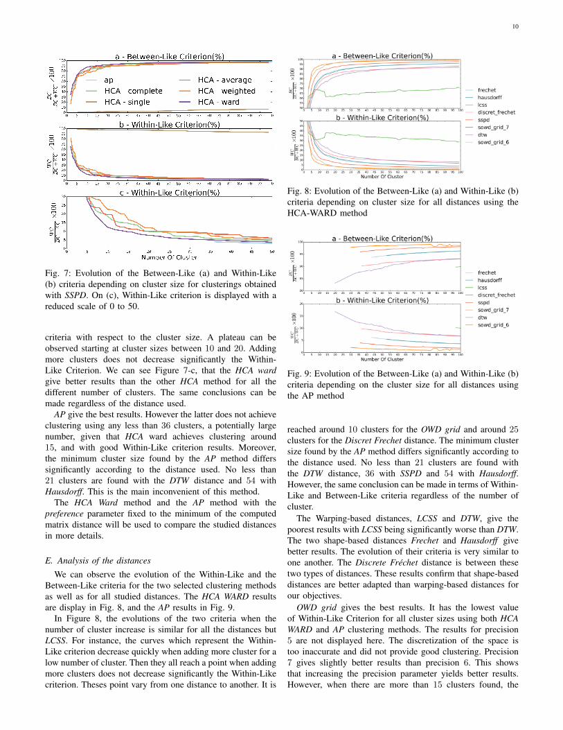
Fig. 7: Evolution of the Between-Like (a) and Within-Like(b) criteria depending on cluster size for clusterings obtainedwith SSPD. On (c), Within-Like criterion is displayed with areduced scale of 0 to 50.

criteria with respect to the cluster size. A plateau can beobserved starting at cluster sizes between 10 and 20. Addingmore clusters does not decrease significantly the Within-Like Criterion. We can see Figure 7-c, that the HCA wardgive better results than the other HCA method for all thedifferent number of clusters. The same conclusions can bemade regardless of the distance used.

AP give the best results. However the latter does not achieveclustering using any less than 36 clusters, a potentially largenumber, given that HCA ward achieves clustering around15, and with good Within-Like criterion results. Moreover,the minimum cluster size found by the AP method differssignificantly according to the distance used. No less than21 clusters are found with the DTW distance and 54 withHausdorff. This is the main inconvenient of this method.

The HCA Ward method and the AP method with thepreference parameter fixed to the minimum of the computedmatrix distance will be used to compare the studied distancesin more details.

E. Analysis of the distances

We can observe the evolution of the Within-Like and theBetween-Like criteria for the two selected clustering methodsas well as for all studied distances. The HCA WARD resultsare display in Fig. 8, and the AP results in Fig. 9.

In Figure 8, the evolutions of the two criteria when thenumber of cluster increase is similar for all the distances butLCSS. For instance, the curves which represent the Within-Like criterion decrease quickly when adding more cluster for alow number of cluster. Then they all reach a point when addingmore clusters does not decrease significantly the Within-Likecriterion. Theses point vary from one distance to another. It is

Fig. 8: Evolution of the Between-Like (a) and Within-Like (b)criteria depending on cluster size for all distances using theHCA-WARD method

Fig. 9: Evolution of the Between-Like (a) and Within-Like (b)criteria depending on the cluster size for all distances usingthe AP method

reached around 10 clusters for the OWD grid and around 25clusters for the Discret Frechet distance. The minimum clustersize found by the AP method differs significantly according tothe distance used. No less than 21 clusters are found withthe DTW distance, 36 with SSPD and 54 with Hausdorff.However, the same conclusion can be made in terms of Within-Like and Between-Like criteria regardless of the number ofcluster.

The Warping-based distances, LCSS and DTW, give thepoorest results with LCSS being significantly worse than DTW.The two shape-based distances Frechet and Hausdorff givebetter results. The evolution of their criteria is very similar toone another. The Discrete Frechet distance is between thesetwo types of distances. These results confirm that shape-baseddistances are better adapted than warping-based distances forour objectives.

OWD grid gives the best results. It has the lowest valueof Within-Like Criterion for all cluster sizes using both HCAWARD and AP clustering methods. The results for precision5 are not displayed here. The discretization of the space istoo inaccurate and did not provide good clustering. Precision7 gives slightly better results than precision 6. This showsthat increasing the precision parameter yields better results.However, when there are more than 15 clusters found, the

11

within and Between-Like criteria are almost the same. Insection VI-C we have seen that the computation time tocompute the distance with precision 7 is seven times higherthan the computation time with precision 6. Hence, we need tolook for the optimal criteria to find a good trade off betweengood clustering results, and reasonable computational time.The choice of this criteria is a strong disadvantage of theOWD method, because it implies to look for the best precisionparameter for each data set.

Finally, the new distance SSDP is the distance which bestapproaches the results found with OWD grid, regardless ofthe number of cluster. But unlike with OWD grid, we do notneed to look for the optimal precision parameter, in order tocompute it, nor to map the trajectory to a new space. Thisenables our distance to be more easily adapted to differentsubsets of trajectories.

We observe the visual results for this distance and bothAP and HCA ward clustering methods, in Fig. 10, and theisolated clusters, in Fig. 11. For the HCA ward method, wedisplay the clustering result obtained with 15 clusters becausewe have seen Section VI-D that a plateau can be observed onthe evolution of the Within-Like criteria with respect to thenumber of cluster starting at cluster sizes between 10 and 20for the SSPD. For the AP, clustering results with 36 clustersis displayed since no less cluster can be obtained with thismethod.

Fig. 10: Clustering results with SSPD distance

We observe that trajectories are well classified accordingto their path. In Fig. 11, clusters found using HCA WARDseem to be consistent. The cluster size with AP method is 36.This is a large number according to the Within-Like criterioncomputed with HCA. In fact, the Within-Like criterion doesnot decrease much between 15 and 36. However, we can seethat the number of clusters found with AP are still consistent.

A cluster computed with the HCA WARD method based ona matrix distance computed with SSPD gives the best result.The Between-Like and Within-Like criteria show that thismethod is best used to regroup cluster around exemplar. Weobtain a partition of the trajectories subset, such as each clusterrepresents a path taken by the drivers. We obtain a partition oftraffic based on the taxi drivers’ behavior leaving the Caltrain

Fig. 11: The isolated clusters

station in San Francisco. The number of trajectories in eachcluster gives us a representation of the importance of eachnetwork traffic stream.

VII. CONCLUSION

Clustering of non Euclidean objects deeply relies on thechoice of a proper distance. For trajectories analysis, wepresented different distances focusing on different featuresof such objects. To cope with their different weaknesseswe propose a new distance, the Symmetrized Segment-PathDistance. This distance is time insensitive, and compares theshape and the physical distance between two trajectory objects.It does not require any additional parameters nor mappingtrajectories in a different space. Hence, It can be appliedon any set of trajectories, regardless of the area they comefrom. It enables us to obtain good clustering using eitherhierarchical clustering and affinity propagation methods. Inthis way, the clusters obtained are homogeneous with regardto shape and seem to properly capture the behaviours of thedrivers. We have thus obtained a partition of the networkbased on the drivers’ usage that can still be interpreted asvehicle trajectories. This partition can be used to solveddifferent problem. Many applications which recommend placesto visit, or which target advertising based on our destinationneed to forecast the final destination of drivers or predict thetravel time of driver trips. Cities which wish to organize tripdistribution of a city, also need to know the behaviours ofthe cars drivers. Some of these problems will be tackled ina following work, based on the partition obtained with ourmethod to cluster trajectories.

ACKNOWLEDGMENTS

We thank the referees for careful reading and numeroussuggestions. They led us to an improvement of the work Wealso thank Frederic and Susan Bejina for helping improve theclarity of the paper.

REFERENCES

[1] S. Gaffney and P. Smyth, “Trajectory clustering with mixtures of regres-sion models,” in Proceedings of the fifth ACM SIGKDD internationalconference on Knowledge discovery and data mining. ACM, 1999, pp.63–72.

[2] D. Vasquez and T. Fraichard, “Motion prediction for moving objects:a statistical approach,” in Robotics and Automation, 2004. Proceedings.ICRA’04. 2004 IEEE International Conference on, vol. 4. IEEE, 2004,pp. 3931–3936.

12

[3] W. Hu, X. Xiao, Z. Fu, D. Xie, T. Tan, and S. Maybank, “A systemfor learning statistical motion patterns,” Pattern Analysis and MachineIntelligence, IEEE Transactions on, vol. 28, no. 9, pp. 1450–1464, 2006.

[4] M. Gariel, A. N. Srivastava, and E. Feron, “Trajectory clustering and anapplication to airspace monitoring,” Intelligent Transportation Systems,IEEE Transactions on, vol. 12, no. 4, pp. 1511–1524, 2011.

[5] S. Rinzivillo, D. Pedreschi, M. Nanni, F. Giannotti, N. Andrienko,and G. Andrienko, “Visually driven analysis of movement data byprogressive clustering,” Information Visualization, vol. 7, no. 3-4, pp.225–239, 2008.

[6] J. Kim and H. S. Mahmassani, “Spatial and temporal characterizationof travel patterns in a traffic network using vehicle trajectories,” Trans-portation Research Part C: Emerging Technologies, vol. 59, pp. 375–390, 2015.

[7] J.-G. Lee, J. Han, and K.-Y. Whang, “Trajectory clustering: a partition-and-group framework,” in Proceedings of the 2007 ACM SIGMODinternational conference on Management of data. ACM, 2007, pp.593–604.

[8] H.-R. Wu, M.-Y. Yeh, and M.-S. Chen, “Profiling moving objects bydividing and clustering trajectories spatiotemporally,” Knowledge andData Engineering, IEEE Transactions on, vol. 25, no. 11, pp. 2615–2628, 2013.

[9] E. Tiakas, A. Papadopoulos, A. Nanopoulos, Y. Manolopoulos, D. Sto-janovic, and S. Djordjevic-Kajan, “Searching for similar trajectories inspatial networks,” Journal of Systems and Software, vol. 82, no. 5, pp.772–788, 2009.

[10] M. K. El Mahrsi and F. Rossi, “Graph-based approaches to clusteringnetwork-constrained trajectory data.” in NFMCP. Springer, 2012, pp.124–137.

[11] B. Han, L. Liu, and E. Omiecinski, “Road-network aware trajectoryclustering: Integrating locality, flow, and density,” Mobile Computing,IEEE Transactions on, vol. 14, no. 2, pp. 416–429, 2015.

[12] J.-R. Hwang, H.-Y. Kang, and K.-J. Li, Spatio-temporal similarityanalysis between trajectories on road networks. Springer, 2005.

[13] D. J. Berndt and J. Clifford, “Using dynamic time warping to findpatterns in time series.” in KDD workshop, vol. 10, no. 16. Seattle,WA, 1994, pp. 359–370.

[14] M. Vlachos, G. Kollios, and D. Gunopulos, “Discovering similar multi-dimensional trajectories,” in Data Engineering, 2002. Proceedings. 18thInternational Conference on. IEEE, 2002, pp. 673–684.

[15] L. Chen and R. Ng, “On the marriage of lp-norms and edit distance,”in Proceedings of the Thirtieth international conference on Very largedata bases-Volume 30. VLDB Endowment, 2004, pp. 792–803.

[16] L. Chen, M. T. Ozsu, and V. Oria, “Robust and fast similarity search formoving object trajectories,” in Proceedings of the 2005 ACM SIGMODinternational conference on Management of data. ACM, 2005, pp.491–502.

[17] B. Lin and J. Su, “Shapes based trajectory queries for moving objects,”in Proceedings of the 13th annual ACM international workshop onGeographic information systems. ACM, 2005, pp. 21–30.

[18] M. M. Deza and E. Deza, Encyclopedia of distances. Springer, 2009.[19] F. Hausdorff, “Grundz uge der mengenlehre,” 1914.[20] M. M. Frechet, “Sur quelques points du calcul fonctionnel,” Rendiconti

del Circolo Matematico di Palermo (1884-1940), vol. 22, no. 1, pp.1–72, 1906.

[21] H. Alt and M. Godau, “Computing the frechet distance between twopolygonal curves,” International Journal of Computational Geometry &Applications, vol. 5, no. 01n02, pp. 75–91, 1995.

[22] T. Eiter and H. Mannila, “Computing discrete frechet distance,” Citeseer,Tech. Rep., 1994.

[23] M. Piorkowski, N. Sarafijanovic-Djukic, and M. Grossglauser, “CRAW-DAD data set epfl/mobility (v. 2009-02-24),” Downloaded fromhttp://crawdad.org/epfl/mobility/, Feb. 2009.

[24] S.-L. Lee, S.-J. Chun, D.-H. Kim, J.-H. Lee, and C.-W. Chung, “Simi-larity search for multidimensional data sequences,” in Data Engineering,2000. Proceedings. 16th International Conference on. IEEE, 2000, pp.599–608.

[25] C.-B. Shim and J.-W. Chang, “Similar sub-trajectory retrieval for movingobjects in spatio-temporal databases,” in Advances in Databases andInformation Systems. Springer, 2003, pp. 308–322.

[26] A. Srivastava, E. Klassen, S. H. Joshi, and I. H. Jermyn, “Shape analysisof elastic curves in euclidean spaces,” Pattern Analysis and MachineIntelligence, IEEE Transactions on, vol. 33, no. 7, pp. 1415–1428, 2011.

Philippe Besse Philippe C. Besse received an En-gineering degree in Computer Science from thePolytechnic Institute of Toulouse, France in 1976and a Ph.D degree in Statistics from the Universityof Toulouse in 1979. He is currently a full Professorin the Department of Mathematics of the InstitutNational des Sciences Appliquees of Toulouse, hav-ing served as Director for the Departement from2007-2013. Prior that, he served as the Directorof the Laboratory of Statistics and Probabilities,University of Toulouse between 2000 and 2005. He

has published more than 50 scientific papers and book chapters in the fieldsof applied Statistics and Biostatistics. His research interests include functionaldata analysis, and the industrial applications of Statistics, Bioinformatics andData Mining.

Brendan Guillouet Brendan Guillouet received hisEngineering degree in Applied Mathematics fromthe Institut National des Sciences Appliquees deToulouse, France in 2013. He is currently doinga CIFRE (Industrial Training and Research) PhD,jointly with Datasio and the Laboratory of Statisticsand Probabilities, University of Toulouse. Its thesisfocusing on Data Mining and Machine Learningmethods applied to mobile data.

Jean-Michel Loubes Jean-Michel Loubes receivedhis Phd of Applied Mathematics at University ofToulouse in 2001. CNRS researcher in statistics atUniversity Paris XI and then Montpellier 2, he issince 2007 a full Professor in the Institute of Math-ematics of the University, having served as Directorfor the Departement of Statistics and Probabilityfrom 2010-2013. He has published more than 50scientific papers and book chapters in the fieldsof applied mathematical Statistics and statisticallearning. His research interests include mathematica

statistics and the industrial applications of Statistics, and Machine Learning.

Francois Royer Francois Royer received his Agron-omy Engineering degree from the Ecole NationaleSuprieure Agronomique de Rennes, after pursueingPhD studies in marine ecology at CLS from 2003 to2005, sponsored by the Centre National des EtudesSpatiales and Ifremer. After a two year post-doctoralposition at the Large Pelagics Research Lab at Uni-versity of New Hampshire, conducting field taggingstudies and working on astronomical geolocationalgorithms, he moved back to the OceanographyDepartment of CLS in 2007 where he actively

worked on underwater geolocation and Argos positioning. He is the author ofnumerous papers specializing in time series analysis, geolocation filtering andsmoothing. He founded Datasio in 2012, a private company focusing on BigData solutions for industrial and environmental applications, where he headsproduct innovation and commercial development. His interests range fromBioinformatics and Data Mining to Domain Specific Language developmentand Functional Programming.