I. Report No. 2. Government Accession No.

FHWNTX-02/4027-1 4. Title and Subtitle

REVIEW AND EVALUATION OFF ACTORS THAT AFFECT THE FREQUENCY OF RED-LIGHT-RUNNING

7. Author(s)

James Bonneson, Marcus Brewer, and Karl Zimmerman 9. Performing Organization Name and Address

Texas Transportation Institute The Texas A&M University System College Station, Texas 77843-3135 12. Sponsoring Agency Name and Address

Texas Department of Transportation Research and Technology Implementation Office P.O. Box 5080 Austin, Texas 78763-5080

15. Supplementary Notes

Technical Rcpon Documentation Page

3. Recipient's Catalog No.

5. Report Date

September 200 I 6. Performing Organization Code

8. Performing Organization Report No.

Report 4027-1 I 0. Work Unit No. (TRAJS)

11. Contract or Grant No.

Project No. 0-4027 13. Type of Report and Period Covered

Research: September 2000 - August 2001 14. Sponsoring Agency Code

Research performed in cooperation with the Texas Department of Transportation and the U.S. Department of Transportation, Federal Highway Administration. Research Project Title: Signalization Countermeasures to Reduce Red-Light-Running 16. Abstract

Red-light-running is a significant problem throughout the United States and Texas. It continues to increase in frequency each year at most intersections and it leads to frequent and severe crashes. Engineering countermeasures represent an attractive means of combating the red-light-running problem because they are intended to help drivers be lawful and they are not punitive (unlike enforcement). The objective of this research project is to describe how traffic engineering countermeasures can be used to minimize the frequency ofred-light-running and associated crashes at intersections.

This report describes findings from the first year of a two-year project. During the first year, studies were conducted ofred-light-running frequency and crash rates at 12 intersection approaches in three Texas cities. The findings from these studies indicate that the frequency ofred-light-running increases in a predictable way with increasing approach volume, increasing heavy-vehicle percentage, and shorter yellow interval durations. The crash data analyses indicate that right-angle crashes increase exponentially with an increasing frequency ofred-light-running. Models for computing an intersection approach's red-light-running frequency and related crash rate are described.

17. Keywords 18. Distribution Statement

Signalized Intersection, Change Interval, Signal Timing Design, Dilemma Zone

No restrictions. This document is available to the public through NTIS:

19. Security Classif.(ofthis report)

Unclassified Fonn DOT F 1700.7 (8-72)

National Technical Information Service 5285 Port Royal Road Springfield, Virginia 22161

20. Security Classif.(of this page)

Unclassified Reproduction of completed page authorized

21. No. of Pages

78 I 22. Price

REVIEW AND EVALUATION OF FACTORS THAT AFFECT THE FREQUENCY OF RED-LIGHT-RUNNING

by

James Bonneson, P .E. Associate Research Engineer Texas Transportation Institute

Marcus Brewer Assistant Transportation Researcher

Texas Transportation Institute

and

Karl Zimmerman Graduate Research Assistant

Texas Transportation Institute

Report 402 7-1 Project Number 0-4027

Research Project Title: Signalization Countermeasures to Reduce Red-Light-Running

Sponsored by the Texas Department of Transportation

In Cooperation with the U.S. Department of Transportation Federal Highway Administration

September 2001

TEXAS TRANSPORTATION INSTITUTE The Texas A&M University System College Station, Texas 77843-3135

---------------------------------------

DISCLAIMER

The contents of this report reflect the views of the authors, who are responsible for the facts and the accuracy of the data published herein. The contents do not necessarily reflect the official view or policies of the Federal Highway Administration and/or the Texas Department of Transportation. This report does not constitute a standard, specification, or regulation. Not intended for construction, bidding, or permit purposes. The engineer in charge of the project was James Bonneson, P.E. #67178.

NOTICE

The United States Government and the State of Texas do not endorse products or manufacturers. Trade or manufacturers' names appear herein solely because they are considered essential to the object of this report.

v

ACKNOWLEDGMENTS

This research project was sponsored by the Texas Department of Transportation (TxDOT) and the Federal Highway Administration. The research was conducted by Dr. James A. Bonneson, Mr. Marcus Brewer, and Mr. Karl Zimmerman with the Design and Operations Division of the Texas Transportation Institute.

The researchers would like to acknowledge the support and guidance provided by the project director, Mr. Wade Odell, and the members of the Project Monitoring Committee, including: Mr. Baltazar Avila, Mr. Dale Barron, Mr. Mike Jedlicka, Mr. James Mercier, Mr. Doug Vanover, Mr. Roy Wright (all with TxDOT), and Mr. Walter Ragsdale (with the City of Richardson). In addition, the researchers would like to acknowledge the assistance provided by Mr. Ismael Soto (with TxDOT) in locating several field study sites and in implementing selected countermeasures. Finally, the valuable assistance provided by Dr. Montasir Abbas in the conduct of this research is also gratefully acknowledged.

Vl

TABLE OF CONTENTS

Page

LIST OF FIGURES ......................................................... viii

LIST OF TABLES ........................................................... ix

CHAPTER 1. INTRODUCTION ............................................. 1-1 OVERVIEW ............................................................ 1-1 RESEARCH OBJECTIVE ................................................. 1-2 RESEARCH SCOPE . . . . . . . . . . . . . . . . . . . . . . . . . . . . . . . . . . . . . . . . . . . . . . . . . . . . . . 1-2 RESEARCH APPROACH ................................................. 1-2

CHAPTER 2. RED-LIGHT-RUNNING PROCESS AND COUNTERMEASURES ... 2-1 OVERVIEW ............................................................ 2-1 EXPOSURE FACTORS ................................................... 2-3 CONTRIBUTORY FACTORS .............................................. 2-6 FACTORS LEADING TO CONFLICT ...................................... 2-13 RED-LIGHT-RUNNING COUNTERMEASURES ............................. 2-15

CHAPTER3. DATA COLLECTION PLAN .................................... 3-1 OVERVIEW ............................................................ 3-1 MODEL DEVELOPMENT ................................................. 3-1 COUNTERMEASURES TO BE EVALUATED ................................ 3-6 SITE SELECTION AND DATA COLLECTION PROCEDURES .................. 3-7

CHAPTER4. DATA ANALYSIS ............................................. 4-1 OVERVIEW ............................................................ 4-1 FACTORS AFFECTING RED-LIGHT-RUNNING .............................. 4-1 EXAMINATION OF CRASH DATA ........................................ 4-17

CHAPTERS. SUMMARY OF FINDINGS ..................................... 5-1 OVERVIEW ............................................................ 5-1 RED-LIGHT-RUNNING PROCESS ......................................... 5-1 RED-LIGHT-RUNNING COUNTERMEASURES .............................. 5-2 FACTORS AFFECTING RED-LIGHT-RUNNING .............................. 5-4 EXAMINATION OF CRASH DATA ......................................... 5-4

CHAPTER6. REFERENCES ................................................ 6-1

APPENDIX: TEXAS TRANSPORTATION CODE CHAPTER 544 ............... A-1

vii

Figure

2-1 2-2 2-3 2-4 2-5 2-6 2-7

2-8 2-9 2-10 3-1 4-1 4-2 4-3 4-4 4-5 4-6 4-7 4-8

4-9

LIST OF FIGURES

Page

Effect of Flow Rate on the Frequency of Red-Light-Running .................... 2-4 Effect of Flow Rate and Detection Design on Max-Out Probability ............... 2-6 Probability of Stopping as a Function of Travel Time and Control Type . . . . . . . . . . . 2-7 Probability of Stopping as a Function of Travel Time and Speed . . . . . . . . . . . . . . . . . 2-8 Probability of Stopping as a Function of Travel Time and Approach Grade . . . . . . . . 2-9 Probability of Stopping as a Function of Travel Time and Yellow Duration . . . . . . . 2-10 Probability of Stopping as a Function of Travel Time and Proximity of Other Vehicles . . . . . . . . . . . . . . . . . . . . . . . . . . . . . . . . . . . . . . . . . . . . 2-11 Variation of Red-Light-Running and Other Conflicts by Time-of-Day ........... 2-13 Relationship Between Probability of Stopping and Yellow Interval Duration . . . . . . 2-14 Relationship Between Red-Light-Running Frequency and Yellow Duration ....... 2-17 Probability of Going at Yellow Onset . . . . . . . . . . . . . . . . . . . . . . . . . . . . . . . . . . . . . . 3-3 Red-Light-Running Frequency as a Function of Approach Volume ............... 4-8 Red-Light-Running Frequency as a Function of Phase-End Flow Rate ............ 4-9 Red-Light-Running Frequency as a Function of Yellow-Interval Duration ........ 4-10 Red-Light-Running Frequency as a Function of Heavy-Vehicle Percentage ....... 4-10 Prediction Ratio versus Predicted Red-Light-Running Frequency ............... 4-13 Comparison of Observed and Predicted Red-Light-Running Frequency .......... 4-14 Predicted Effect of Flow Rate on Red-Light-Running Frequency ................ 4-16 Predicted Effect of Yellow Duration and Vehicle Mix on Red-Light-Rutining Frequency .......................................... 4-17 Predicted Effect of Red-Light-Running on Intersection Crashes ................. 4-20

viii

LIST OF TABLES

Table Page

2-1 Events Leading to Red-Light-Running and Related Crashes . . . . . . . . . . . . . . . . . . . . . 2-1 2-2 Factors Affecting Driver Decision at Onset of Yellow Indication ................. 2-7 2-3 Relationship Between Countermeasure Category and Driver Type . . . . . . . . . . . . . . 2-16 2-4 Engineering Countermeasures to Red-Light-Running ......................... 2-17 3-1 Red-Light-Running-Related Measures of Effectiveness ........................ 3-1 3-2 Intersection Characteristics .............................................. 3-9 3-3 Candidate Study Site Characteristics ...................................... 3-10 3-4 Proposed Countermeasure at Each Study Site . . . . . . . . . . . . . . . . . . . . . . . . . . . . . . . 3-11 3-5 Database Elements .................................................... 3-12 4-1 Database Summary - Geometric and Traffic Control Variables . . . . . . . . . . . . . . . . . . 4..:2 4-2 Database Summary- Total Observations .................................... 4-2 4-3 Database Summary - Statistics for Selected Variables ......................... 4-3 4-4 Red-Light-Running Rates at Each Study Site ................................ 4-7 4-5 Calibrated Red-Light-Running Model Statistical Description ................... 4-12 4-6 Propensity (P,) for Selected Heavy-Vehicle Percentages and Yellow Durations .... 4-15 4-7 Crash Frequency at Each Study Site . . . . . . . . . . . . . . . . . . . . . . . . . . . . . . . . . . . . . . 4-18 4-8 Calibrated Crash Model Statistical Description .............................. 4-19 5-1 Engineering Countermeasures with Greatest Potential . . . . . . . . . . . . . . . . . . . . . . . . . 5-3

lX

CHAPTER 1. INTRODUCTION

OVERVIEW

When a traffic signal changes from a green indication to a yellow indication, the approaching driver must decide to either initiate a stop before the intersection or continue through the intersection. If the driver decides to stop, it is because he or she has determined that there is insufficient time to reach the intersection before the change to a red indication. If the driver decides to continue (or "go"), the reason is less clear. It may be that the driver has determined that: (1) a safe stop is not possible, (2) a comfortable stop is not possible, or (3) it is inconvenient to stop. Alternatively, the driver may simply not be aware of the need to stop. Regardless of the reason, if the "going" driver's arrival to the intersection occurs after the indication has changed to red, then the driver is said to have "run the red light."

Statistics indicate that red-light-running has become a significant safety problem throughout the United States. Retting et al. (J) report that about one million collisions occur at signalized intersections in the U.S. each year. Of these collisions, Mohamedshah et al. (2) estimate that at least 16 to 20 percent can be attributed directly to red-light-running. Retting et al. also report that motorists involved in red-light-running-related crashes are more likely to be injured than in other crashes. In fact, they found that 45 percent of red-light-running-related crashes involve injury whereas only 30 percent of other crashes involve injury.

A 1998 survey of Texas drivers by the Federal Highway Administration (FHW A) (3) found that two of three Texans witness red-light-running every day. About 89 percent of these drivers believe that red-light-running has worsened over the past few years. The largest percentage (66 percent) perceive the reason for red-light-running is that the red runner is "in a hurry." An examination of nationwide fatal crash statistics by the Insurance Institute for Highway Safety found that Texas has the fourth highest number of red-light-running-related deaths per 100,000 population (4).

There is a wide range of potential countermeasures to the red-light-running problem. These solutions are generally divided into two broad categories: engineering countermeasures and enforcement countermeasures. Enforcement countermeasures are intended to encourage drivers to adhere to the traffic laws through the threat of citation and possible fine. In contrast, engineering countermeasures (which include any modification, extension, or adjustment to an existing traffic control device) are intended to reduce the chances of a driver being in a position where he or she must decide whether or not to run the red. Studies by Retting et al. (J) have shown that countermeasures in both categories are effective in reducing the frequency of red-light-running. However, most of the research conducted to date has focused on the effectiveness of enforcement; little is known about the effectiveness of many engineering countermeasures.

In summary, red-light-running is a significant problem throughout the United States and Texas. It appears to be a growing problem and it leads to frequent and severe crashes. Engineering

1-1

countermeasures represent an attractive means of combating the red-light-running problem as they are passively applied (in that they attempt to help drivers be lawful); however, more research is needed to identify the range of countermeasures available and their potential effectiveness.

This report describes the extent of the red-light-running problem as well as several countermeasures that have been used to reduce the frequency of red-light-running and associated right-angle collisions. Initially, there is an examination of the red-light-running process in terms of the events necessary to precipitate a red-light-running event. Then the effectiveness of various countermeasures is discussed. Next, a model for predicting the frequency of red-light-running is developed and used to defme a data collection plan. This development is followed by an analysis of red-light-running data and an analysis of crash history data. Finally, the findings from both of these analyses are summarized.

RESEARCH OBJECTIVE

The objective of this research project is to describe how traffic engineering countermeasures can minimize the frequency of red-light-running and associated crashes at intersections. This objective will be achieved through satisfaction of the following goals:

1. Quantify the effect of various traffic and control factors on frequency of red-light-running. 2. Quantify the relationship between red-light-running and crash frequency. 3. Identify promising engineering countermeasures and quantify their effects. 4. Facilitate implementation of engineering countermeasures through development of a guide.

The research conducted during the first year of the project was focused on fulfilling the first two goals.

RESEARCH SCOPE

This research project deals exclusively with engineering countermeasures to the red-light­running problem. These countermeasures and their associated application guidelines are developed for use at urban and suburban signalized intersections.

RESEARCH APPROACH

This project's research approach is based on a two-year program of development and evaluation that will ultimately yield a guideline document for identifying and deploying effective engineering countermeasures. During the first year of the research, the causes ofred-light-running and its effect on safety has been quantified. In the second year, the most promising countermeasures will be implemented and evaluated. The main product of this research will be a guideline document. This document will provide technical guidance for engineers interested in using engineering countermeasures to reduce red-light-running in a cost-effective manner. It will also provide quantitative information on the effectiveness of each countermeasure.

1-2

OVERVIEW

CHAPTER 2. RED-LIGHT-RUNNING PROCESS AND COUNTERMEASURES

This chapter describes the red-light-running process and the countermeasures described in the literature as having some effect on the frequency of red-light-running. Initially, the red-light­running process is described in terms of the events that lead to red-light-running and the factors that have some influence on a driver's propensity to run the red light. The chapter concludes with a discussion of red-light-running countermeasures with a focus on those described as "engineering" countermeasures.

Red-Light-Running Process

Several events must occur together to result in a driver entering the intersection after the change from a yellow to a red indication. Table 2-1 lists these events in roughly the same sequence that they must occur to lead to a red-run event.

T bl 2 1 E t L d. a e - . ven s ea mg to Rd L" ht R e - 12 - unnm2an dRI dC h e ate ras es. Type Event RLR Rt. Angle Rear-end

Freq Crash Crash

Exposure 1. Vehicle i is x sec. travel time from the intersection (x < 6 s ). .,. .,. .,. Events 2. Phase terminates (yellow presentation). .,. .,. .,.

3. Phase termination is by phase max-out (or controller is pretimed). .,. .,. .,. Contrib- 4. Vehicle i does not stop. .,. .,. .,. utory 5. Vehicle i's entry time occurs after yellow ends. .,. .,. Events

6. Vehicle i's clearance time occurs after all-red ends. .,. 7. Conflicting vehicle k enters intersection y sec. after all-red ends. .,. 8. Vehicle} stops (and it is in front of vehicle i). .,.

Note: RLR =red-light-running

The first three events listed in Table 2-1 represent exposure events because they "set the stage" for the contributory events that follow. Thus, exposure to red-light-running requires: (1) sufficient traffic volume to result in one or more vehicles on the intersection approach; (2) a

.phase termination; and (3) pretimed control or, if the control is actuated and advance detection is used, the termination is by "max-out" (i.e., maximum green limit is reached). Consideration of the first two events suggests that exposure to red-light-running increases with flow rate on the subject approach and the number of signal cycles.

2-1

The contributory events that lead to red-light-running include: (1) the vehicle does not stop, and (2) the vehicle's time of entry to the intersection occurs after the indication changes from yellow to red. Consideration of these two events suggests that the frequency of red-light-running will increase whenever drivers are less likely to stop and when the yellow interval is reduced.

The "vehicle does not stop" event is the most complex event of those listed in Table 2-1. The probability of this event is discussed herein in terms of its inverse, the probability of stopping. It reflects the uncertainty (or indecision) exhibited by the population of drivers on an intersection approach at the onset of the yellow indication. The associated event is complex because many factors can affect the probability of stopping (e.g., travel time to intersection, speed, etc.). A subsequent section of this report discusses these factors in more detail.

The last two columns of Table 2-1 relate to the two types of crashes most commonly found at signalized intersections. Both types require the same exposure events. The right-angle crash also requires: (1) the clearing vehicle to be present in the intersection when the all-red ends, and (2) a conflicting vehicle to enter the intersection while it is occupied by the clearing vehicle. Consideration of these two events suggests that the frequency of right-angle crashes increases with a decrease in the all-red interval and an increase in the conflicting movement flow rate.

Based on the preceding discussion, the following factors are believed to influence the frequency of red-light-running and related crash frequency:

• flow rate on the subject approach (exposure factor), • number of signal cycles (exposure factor), • phase termination by max-out (exposure factor), • probability of stopping (contributory factor), • yellow interval duration (contributory factor), • all-red interval duration (contributory factor), • entry time of the conflicting driver (contributory factor), and • flow rate on the conflicting approach (exposure factor).

Each of these factors is described more fully in a subsequent section.

Review of Texas Law

To provide some perspective on the problem of red-light-running in Texas, it is important to be familiar with the applicable laws, codes, and ordinances. Chapter 544 of the Texas Transportation Code (5) deals with traffic signs, signals, and markings; section 544.007 specifically addresses traffic-control signals. The text of this section is listed in the Appendix; the relevant passages are discussed in this section.

Section 544.007 is somewhat ambiguous concerning the specific problem of red-light­running, in that the definition of a driver's responsibility when encountering a yellow signal is not

2-2

fully specified. According to Subsection (b ), a driver waiting at an intersection when his or her signal turns green must wait until all other legally-entering vehicles have cleared the intersection before proceeding. Therefore, Texas law implies that a vehicle that enters an intersection legally (i.e., during yellow) may still be in the intersection after a conflicting movement receives a green signal.

This law is sometimes referred to as the "permissive yellow rule" in comparison to more restrictive laws that require drivers to have exited the intersection before the end of the yellow interval. Parsonson et al. ( 6) indicate that at least half of the states in the United States follow the permissive rule. The advantage of the permissive rule is that it enables most drivers to be lawful in their responses to the yellow indication.

The disadvantage of the permissive rule is that it creates a situation where the cross street driver (or pedestrian) will receive a green indication but must yield the right-of-way before entering the intersection. Parsonson et al. indicate that 60 percent of drivers are unaware that they have to yield the right-of-way when presented the green indication. Moreover, when asked the following question, "What would you think if traffic engineers decided to time yellow lights so that there might be a vehicle going through the intersection when you get your green?" 69 percent of drivers said that they disapproved because it sounded dangerous. The solution advocated by Parsonson et al. was to provide an all-red interval (following the yellow interval) that was of sufficient duration to permit traffic to clear the intersection before a conflicting phase was presented with a green indication.

EXPOSURE FACTORS

This section summarizes the literature as it relates to events that expose drivers to conditions that may precipitate red-light-running. These events were previously discussed with regard to Table 2-1. The factors that underlie these events include flow rate, number of signal cycles, and phase termination by max-out.

Flow Rate on the Subject Approach

Flow rate on the subject approach is important to the discussion of red-light-running. Each vehicle on the intersection approach at the onset of yellow is exposed to the potential for red-light­running. The number of drivers running the red each signal cycle will likely increase as the flow rate increases.

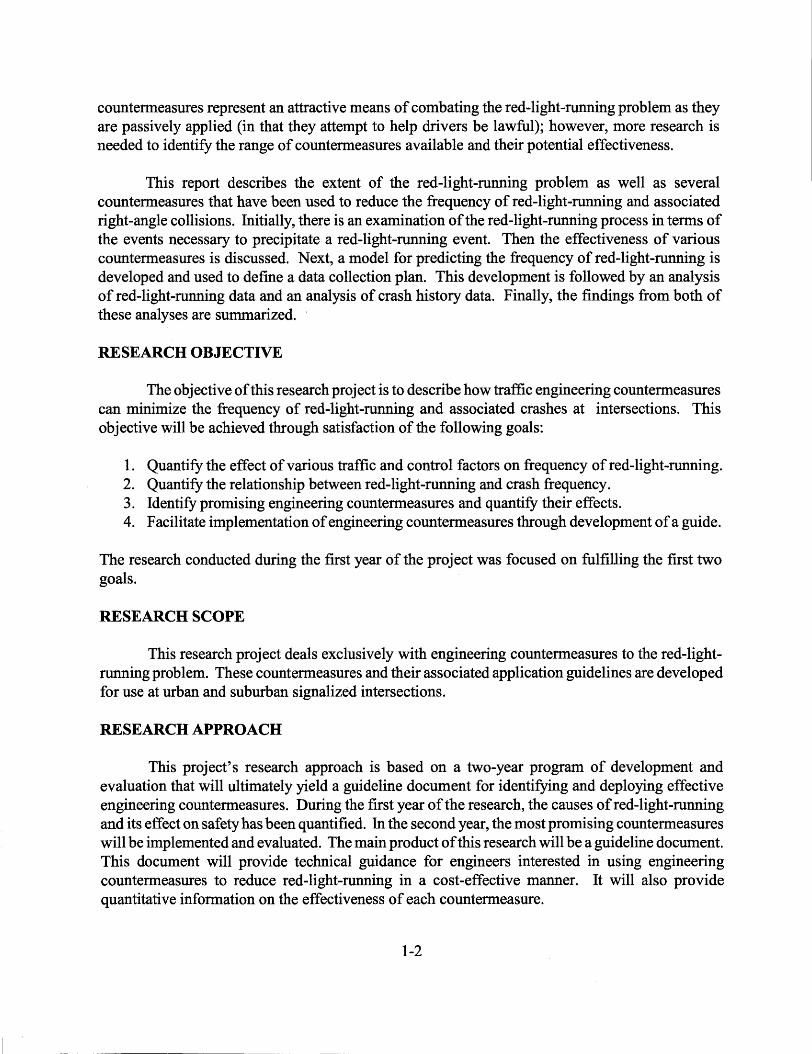
Three studies have considered the effect of flow rate on red-light-running frequency or related crashes. Porter and England (7) observed 5,112 signal cycles at six urban intersections in three Virginia cities. They found that about 35 percent of the observed cycles had at least one red­light-runner. They also noted that intersections with higher volumes were associated with a higher percentage of cycles with red-light-running. This trend is shown in Figure 2-1 (using square data points); it is based on an analysis of the data reported by Porter and England. The "best-fit" trend

2-3

line is labeled "urban, no advance detection." The lack of advance detection was assumed based on the urban-street location of the intersections studied.

>-()

c Cl.I ::I er Cl.I ...

LL. tn .5 .c -c .c c Cl.I ::I > a:

I .. .c . !i?» ..I

I

"D Cl.I a:

30

25 ~ ..................... • ......... I i

20 !

15 ~ : : : : : uman, no advance detection: : : : : • : : : : : : :

10 ~ - - - - - - - - - - - - -.- - - - - - - - - - - - - - - - - -! Rural with advance detection

5 ~ - - - - - - - - - •• - - - -

I • • 0

• • •

0 200 400 600 800 1 ,000 1 ,200 1 ,400

Approach Volume, veh/h

Figure 2-1. Effect of Flow Rate on the Frequency of Red-Light-Running.

Baguley ( 8) examined the frequency of red-light-running at seven rural intersections in England. Each intersection had advance detectors that extended the green indication when vehicles were on the approach. Baguley found that the red-light-running frequency correlated with the approach volume. It also correlated with the number of signal cycles (to be discussed next), approach speed, and the length of the signal cycle. The relationship between flow rate and red-light­running frequency for six of the seven intersections is shown in Figure 2-1 (using circular data points). The six intersections shown had approach speeds of 52 to 67 mph; The seventh intersection had an approach speed well above this range and did not follow the trend shown in Figure 2-1.

Mohamedshah et al. (2) examined the effect of flow rate (and other variables) on red-light­running-related crashes. They obtained crash data for 1,756 urban intersections in California. The data were screened to include only those crashes attributable to a red-light-running event. They found that crash frequency increased with flow rate on the subject approach. Their findings indicate that approach crash frequency increases from 0.25 crash/yr at a two-way volume of 8,000 veh/day to 0.5 crash/yr at 50,000 veh/day.

2-4

Number of Signal Cycles

As noted previously, most researchers recognize that the frequency of red-light-running and associated crashes is largely affected by the frequency with which the yellow indication is presented (7, 8, 9). If the cycle length changes from 60 to 120 s, the number of times that yellow is presented is reduced by 50 percent. A similar reduction in red-light-running frequency should also be observed. Recognition of this relationship is often exhibited by the researchers reporting red-light­running statistics normalized by cycle frequency. For example, Porter and England (7) use "percent of cycles with at least one red-light-runner." Van der Horst and Wilmink (9) use a similar statistic in their work.

Phase Termination by Max-Out

Green-extension detection systems use one or more detectors located in advance of the intersection to hold the green as long as the approach is occupied. By holding the green, drivers are not exposed to the yellow indication and the potential need to red-light-run. However, ifthe green is held to its maximum limit, the phase "maxes-out" and is forced to end, regardless of whether a vehicle is approaching the intersection. An actuated phase that maxes-out (or any pretimed phase) has the potential to expose more drivers to a red-light-running situation than does an actuated phase that ends by gap-out.

Evidence of the effect of a green-extension system (i.e., advance detection) on red-light­running frequency is indicated in Figure 2-1. The trend lines indicate green-extension systems are associated with a lower incidence of red-light-running at a given volume level. Zegeer and Deen (10) also evaluated the effect of green-extension systems on the frequency of red-light-running. Their study revealed a 65 percent reduction in red-running frequency due to the use of a green­extension system.

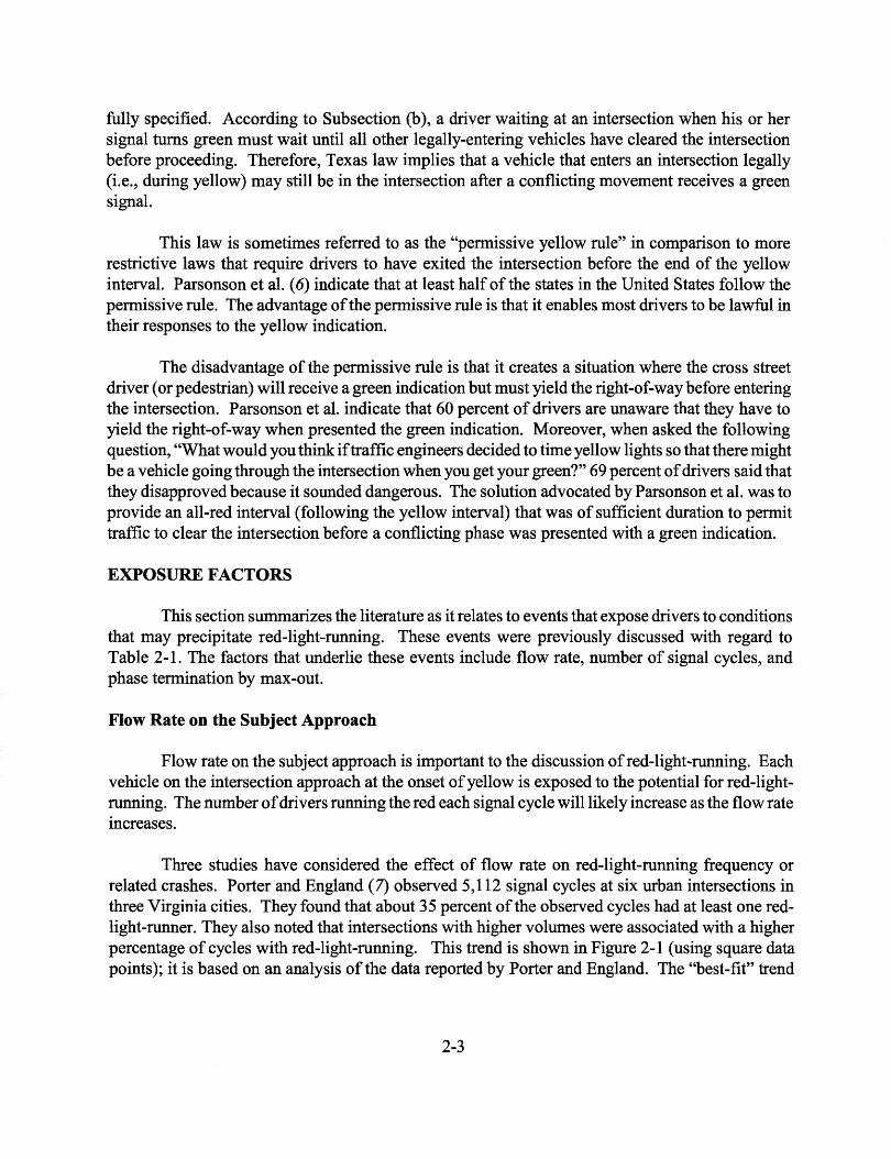
The benefits of green-extension can be negated if the phase maxes-out. The probability of max-out is dependent on flow rate in the subject phase and the "maximum allowable headway," as dictated by the detector design. The maximum allowable headway (MAH) is the largest headway in the traffic stream that can occur and still sustain a continuous extension of the green interval. The relationship between max-out probability, MAH, maximum green, and flow rate is illustrated in Figure 2-2.

Bonneson and McCoy (11) indicate that the MAH values shown in Figure 2-2 (i.e., 4.0 and 7 .0 s) represent the range of values for most detection designs. To illustrate the implications of alternative MAH values, consider the following example. If a phase has a flow rate of 1,200 veh/hr, a maximum green duration of 30 s, and no advance detection (i.e., only a stop-line loop) yielding a MAH of only 4.0 s, then its probability of max-out will be about 0 .05 ( 1 out of 20 cycles). However, if a green-extension system is used, then the MAH will likely be about 7 .0 s and the resulting max­out probability will increase to 0.7 (7 out of 10 cycles). One option available to reduce this

2-5

probability is to increase the maximum green setting; however, this increase may also increase the delay to waiting vehicles.

.. ~

0 I

>< m :E

Jl m Jl 0 ...

D..

1.0 - 30-s Maximum Green

O.S ~ ".""" ":" 50-s Maximum Green ... _ .. _ . _ .

0.6 r- -----------~d~a~~e-D-et-e~ti~~ - - -

! (7.0 s MAH) I

0.4 1 · ...... ~o0A6d:::~ ~et~c~i~n . - - - . - / .. - l

0.2 1- -------------------i

0.0

0 200 400 600 800 1 ,000 1 ,200 1 ,400

Total Flow Rate in Subject Phase, veh/h

Figure 2-2. Effect of Flow Rate and Detection Design on Max-Out Probability.

CONTRIBUTORY FACTORS

Two factors underlie the events that contribute to red-light-running. These factors include the probability of stopping and the yellow interval duration. The former factor represents the complex decision-making process that drivers exhibit at the onset of yellow. A review of the literature indicates that this decision is affected by the driver's assessment of the prevailing traffic and roadway conditions and by his or her estimate of the consequences of stopping (or not stopping). The yellow interval duration contributes in a more fundamental manner. The start of this interval defines the instant when the "signal" to stop is presented. The end of this interval defines the instant when the red indication is presented (whereupon entry to the intersection represents a red-light­running event). Both factors, and their relationship to the frequency of red-light-running, are described in this section.

Probability of Stopping

Many researchers have studied the decision to stop in response to the yellow indication. Van der Horst et al. (9) studied this decision process and found that a driver's propensity to stop is based on three components. These components and the factors that influence them are listed in Table 2-2. Each component is discussed in the following subsections.

2-6

T bl 2 2 F t a e - . ac ors Affi ti D . ec n2 river D .. t 0 t f Y II I d" t" ec1s1on a nse 0 e ow n 1ca ion. Components of the Decision Process Factor

Driver behavior Travel time Speed Actuated control Coordination Approach grade Yellow interval Headway

Estimated consequences of not stopping Threat of right-angle crash Threat of citation

Estimated consequences of stopping Threat of rear-end crash Expected delay

Driver Behavior

Driver behavior embraces many elements of the human psyche as it relates to the expectancy­response system. Driver response to the yellow indication is affected by the driver's awareness of, attitude toward, and ability to estimate the effects of the seven factors listed in Table 2-2. Each of these factors is discussed in the following paragraphs.

Travel Time. A driver's assessment of the probability of stopping requires accurate estimates of speed and distance to the stop line. Through these estimates, a driver assesses his or her ability to stop and the degree of comfort associated with the stop. Several researchers have measured driver response to the yellow indication in terms of the travel time to the intersection at the onset of yellow (9, 12, 13, 14, 15, 16). The relationships reported by these researchers are shown in Figure 2-3.

1.0

en .5 0.8 a. a. 0 u; 0.6 -0

·-~- 0.4 .a m .a 0 D:. 0.2

0.0

0

Olson & Rothery (12)

.. t ._ •••• Actuated

______ H_ulsher (_14)_ __ _ . .. -,- - - 7- - - -- Pretimed

Sheffi &

30 mph

t

• - --~~~- - - - - - - - - - - - - -

' ,.'-......___Bonneson et al. (16) ' $ / ~

- - ~;-. ~' van-der-Horst- & w ilmin-k -<9> -..... _,-- ... = $ -

2 3 4 5 6

Travel Time to Stop Line, s

7

Figure 2-3. Probability of Stopping as a Function of Travel Time and Control Type.

2-7

The trends in Figure 2-3 indicate that the probability of stopping varies with travel time. They also indicate that there is a range, between about 2 and 5-s travel-time from the intersection stop line, where drivers collectively are indecisive about the decision to stop. The solid and dashed lines suggest that there is a difference in driver behavior at pretimed and at actuated intersections. This trend is discussed in the section titled Actuated Control and Coordination.

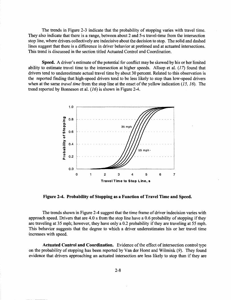
Speed. A driver's estimate of the potential for conflict may be skewed by his or her limited ability to estimate travel time to the intersection at higher speeds. Allsop et al. ( 17) found that drivers tend to underestimate actual travel time by about 30 percent. Related to this observation is the reported finding that high-speed drivers tend to be less likely to stop than low-speed drivers when at the same travel time from the stop line at the onset of the yellow indication (15, 16). The trend reported by Bonneson et al. (16) is shown in Figure 2-4.

1.0

m 0.8 .!: a. a. 0 - 0.6 en .... 0 >.

~ 0.4 .c as .c 0

0.2 ... a.

0.0

0 2 3 4 5 6 7

Travel Time to Stop Line, s

Figure 2-4. Probability of Stopping as a Function of Travel Time and Speed.

The trends shown in Figure 2-4 suggest that the time frame of driver indecision varies with approach speed. Drivers that are 4.0 s from the stop line have a 0.6 probability of stopping if they are traveling at 35 mph; however, they have only a 0.2 probability if they are traveling at 55 mph. This behavior suggests that the degree to which a driver underestimates his or her travel time -increases with speed.

Actuated Control and Coordination. Evidence of the effect of intersection control type on the probability of stopping has been reported by Van der Horst and Wilmink (9). They found evidence that drivers approaching an actuated intersection are less likely to stop than if they are

2-8

approaching a pretimed intersection. They rationalized that drivers learn which signals are actuated and then develop an expectation of service if they are "in queue" near the end of the phase. This effect of control type on the probability-of-stopping is shown in Figure 2-3.

Van der Horst and Wilmink (9) extrapolated the aforementioned expectancy for green to drivers traveling within platoons through a series of interconnected signals. These drivers develop an ad hoc expectancy as they travel without interruption through successive signals. Their expectancy would be that the next signal will remain green until after they (and the rest of the platoon) pass through the intersection. As a result, they are optimistic when the yellow is presented that it will stay yellow long enough for them to stay with the platoon.

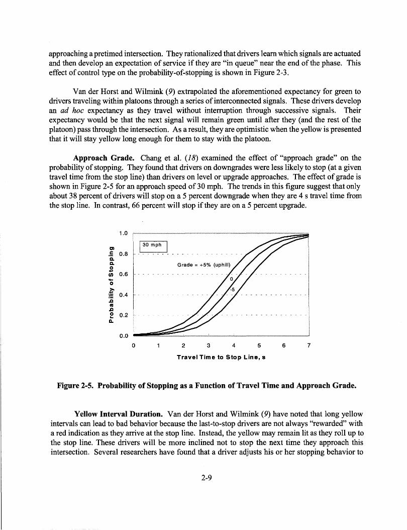
Approach Grade. Chang et al. ( 18) examined the effect of "approach grade" on the probability of stopping. They found that drivers on downgrades were less likely to stop (at a given travel time from the stop line) than drivers on level or upgrade approaches. The effect of grade is shown in Figure 2-5 for an approach speed of 30 mph. The trends in this figure suggest that only about 3 8 percent of drivers will stop on a 5 percent downgrade when they are 4 s travel time from the stop line. In contrast, 66 percent will stop if they are on a 5 percent upgrade.

1.0 I

m ~ 130 mph I

! O.B Grade= +5% (uphill) 0 ~ 0.61 · . . . . . . . . . . . . . . . . . . . . ~ 0.4 r- - - - - - - - - - - - - - - -

~ I £ 0.2 1- ----------I

0.0

0 2 3 4 5 6 7

Travel Time to Stop Line, s

Figure 2-5. Probability of Stopping as a Function of Travel Time and Approach Grade.

Yellow Interval Duration. Van der Horst and Wilmink (9) have noted that long yellow intervals can lead to bad behavior because the last-to-stop drivers are not always "rewarded" with a red indication as they arrive at the stop line. Instead, the yellow may remain lit as they roll up to the stop line. These drivers will be more inclined not to stop the next time they approach this intersection. Several researchers have found that a driver adjusts his or her stopping behavior to

2-9

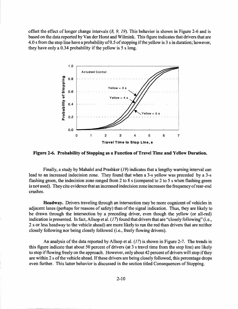
offset the effect of longer change intervals ( 8, 9, 19). This behavior is shown in Figure 2-6 and is based on the data reported by Van der Horst and Wilmink. This figure indicates that drivers that are 4.0 s from the stop line have a probabilityof0.5 of stopping if the yellow is 3 sin duration; however, they have only a 0.34 probability ifthe yellow is 5 s long.

1.0

m .5 0.8 a. a. 0 u; 0.6 -0 >a E o.4 .c ca .c 0 ~ 0.2

0.0

0

Actuated Control

Yellow= 3 s

Yellow= 4 s

2 3 4 5 6 7

Travel Time to Stop Line, s

Figure 2-6. Probability of Stopping as a Function of Travel Time and Yellow Duration.

Finally, a study by Mahalel and Prashker ( 19) indicates that a lengthy warning interval can lead to an increased indecision zone. They found that when a 3-s yellow was preceded by a 3-s flashing green, the indecision zone ranged from 2 to 8 s (compared to 2 to 5 s when flashing green is not used). They cite evidence that an increased indecision zone increases the frequency of rear-end crashes.

Headway. Drivers traveling through an intersection maybe more cognizant of vehicles in adjacent lanes (perhaps for reasons of safety) than of the signal indication. Thus, they are likely to be drawn through the intersection by a preceding driver, even though the yellow (or all-red) indication is presented. In fact, Allsop et al. (17) found that drivers that are "closely following" (i.e., 2 s or less headway to the vehicle ahead) are more likely to run the red than drivers that are neither closely following nor being closely followed (i.e., freely flowing drivers).

An analysis of the data reported by Allsop et al. (17) is shown in Figure 2-7. The trends in this figure indicate that about 50 percent of drivers (at 3 s travel time from the stop line) are likely to stop if flowing freely on the approach. However, only about 42 percent of drivers will stop if they are within 2 s of the vehicle ahead. If these drivers are being closely followed, this percentage drops even further. This latter behavior is discussed in the section titled Consequences of Stopping.

2-10

m .5 0.8 CL CL 0 u; 0.6 .... 0 >

.'!::::: 0.4

.a ca .a ~ 0.2

Q.

9 -Subject vehicle

Free flow vehicle

--~-·~------0.0 l...-----&ii:::~~~-----~----____J

0 2 3 4 5 6 7

Travel Time to Stop Line, s

Figure 2-7. Probability of Stopping as a Function of Travel Time and Proximity of Other Vehicles.

Consequences of Not Stopping

In addition to the various factors that affect driver behavior, there are also several factors that the driver explicitly assesses when deciding on a response to the yellow indication. This assessment includes consideration of the consequences of not stopping and the consequences of stopping. The former consideration includes an estimate of the potential for a right-angle crash and the potential for receiving a citation. The latter consideration is discussed in the section titled Consequences of Stopping.

Threat of Right-Angle Crash. A driver contemplating running the red may assess the threat of a right-angle crash by estimating the number of vehicles in the conflicting traffic stream. This number may be estimated by scanning the intersection ahead and by recalling prior experience at this intersection. A study by Baguley ( 8) found a significant correlation between the frequency of red­light-running and the volume of the conflicting movements. His data indicate that drivers are six times more likely to run the red when the minor road has a daily traffic volume of 2,000 veh/day compared to when it has 17,000 veh/day.

Threat of Citation. Van der Horst and Wilmink (9) noted that drivers consider the potential for being cited when deciding whether to run a red light. The results from a survey of drivers conducted by Retting and Williams (20) support this claim. They found that 46 percent of drivers (in cities without camera enforcement) believe that someone who runs a red light is likely to be given a citation. This percentage increases to 61 percent in cities with camera enforcement.

2-11

Consequences of Stopping

A driver's concern about a possible rear-end crash and lengthy delay is also factored into the decision to stop when presented with a yellow indication.

Threat of Rear-End Crash. Drivers that are being closely followed when the light turns from green to yellow may be more reluctant to stop because of the greater likelihood of a rear-end crash. In a laboratory setting, Allsop et al. (17) observed that drivers being closely followed (i.e., when the following vehicle's headway was less than 2 s) at the onset of yellow were more likely to run the red.

Figure 2-7 shows the effect close following on the probability-of-stopping. The trends in this figure indicate that about 50 percent of drivers (at 3 s travel time from the stop line) are likely to stop if flowing freely on the approach. However, only about 25 percent of drivers will stop if they are being closely followed. This percentage drops to 8 percent when the driver is both closely followed and closely following another vehicle.

Expected Delay. A survey conducted by the FHWA (3) indicated that 66 percent of Texas drivers believe red-light-running is due to drivers who are in a hurry. Obviously, the delay associated with stopping is contrary to most driver's desire to reach his or her destination quickly.

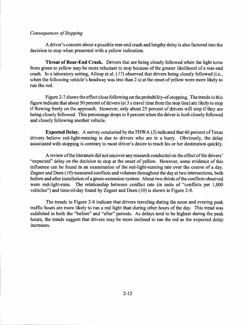
A review of the literature did not uncover any research conducted on the effect of the drivers' "expected" delay on the decision to stop at the onset of yellow. However, some evidence of this influence can be found in an examination of the red-light-running rate over the course of a day. Zegeer and Deen ( 10) measured conflicts and volumes throughout the day at two intersections, both before and after installation of a green-extension system. About two-thirds of the conflicts observed were red-light-runs. The relationship between conflict rate (in units of "conflicts per 1,000 vehicles") and time-of-day found by Zegeer and Deen (10) is shown in Figure 2-8.

The trends in Figure 2-8 indicate that drivers traveling during the noon and evening peak traffic hours are more likely to run a red light than during other hours of the day. This trend was exhibited in both the "before" and "after" periods. As delays tend to be highest during the peak hours, the trends suggest that drivers may be more inclined to run the red as the expected delay increases.

2-12

~ 25 ~~~~~~~~~~~~~~~~~~~~ ~ 'Io Before advance detection •After advance detection : > I •

0 & 20 - - - - - - - - - - - - - - - -- - - - - - - - - - - - -

:i::: en .. . ~ 15 -:;:: c 0 ()

~ 10 - - - -.. ca a: ~ 5 -

- - - - - - - - --

~ o~--------_.__.__.._.~~_._..~~1L-...<-_I~.__.__. 8 9 10 11 12 2 3 4 5

Time of Day

Figure 2-8. Variation of Red-Light-Running and Other Conflicts by Time-of-Day.

Yellow Interval Duration

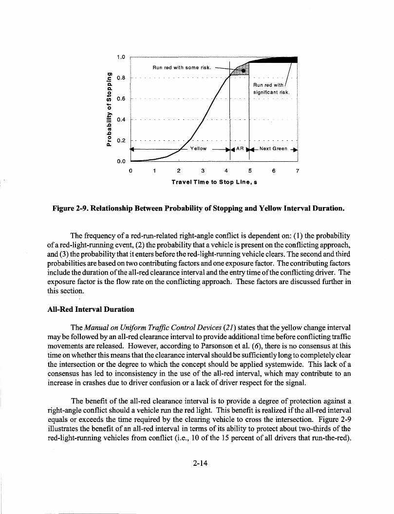
The yellow interval duration is generally recognized as a key factor that affects the frequency ofred-light-running. This recognition has led several researchers to recommend setting the yellow interval duration based on the probability of stopping (9, 12, 18). These researchers suggest that the yellow interval should be based on the g5th (or 90th) percentile driver's travel time to the stop line. This approach is illustrated in Figure 2-9 where the trends shown suggest that a yellow interval of 4.2 s is sufficient for 85 percent of drivers. Only 15 percent of drivers would choose to run the red if they are more than 4.2-s travel time from the stop line at the onset of yellow and are in the "first­to-stop-position."

FACTORS LEADING TO CONFLICT

Once the driver has been exposed to the potential for a red-light-run event and has chosen not to stop at the onset of yellow, there is a threat of conflict with other vehicles. This conflict can lead to a crash if one or both drivers are unable to effect an evasive maneuver. The frequency of a rear-end conflict (that occurs when the lead driver decides to stop and the following driver decides not to stop) is dependent on: (1) the probability of a red-light-running event, (2) the probability that two vehicles are present on the subject approach, and (3) the probability that the driver of the lead vehicle chooses to stop. The second probability is based on the flow rate on the subject approach as a contributing factor. The first and third probabilities were the subject of the preceding section.

2-13

1.0

0) 0.8 .5

c. c. 0 - 0.6 en -0 >-~ 0.4 .a ca .a 0 0.2 ...

CL.

0.0

0

Run red with some risk.

-~.-AR

2 3 4 5

Run red with

significant risk. j - - - - - - - - - -:

'

- - - - - - - - - _\

~ - - - - - - - - -1 i

Next Green -.i i

6 7

Travel Time to Stop Line, s

Figure 2-9. Relationship Between Probability of Stopping and Yell ow Interval Duration.

The frequency of a red-run-related right-angle conflict is dependent on: (1) the probability of a red-light-running event, (2) the probability that a vehicle is present on the conflicting approach, and (3) the probability that it enters before the red-light-running vehicle clears. The second and third probabilities are based on two contributing factors and one exposure factor. The contributing factors include the duration of the all-red clearance interval and the entry time of the conflicting driver. The exposure factor is the flow rate on the conflicting approach. These factors are discussed further in this section.

All-Red Interval Duration

The Manual on Uniform Traffic Control Devices (21) states that the yellow change interval may be followed by an all-red clearance interval to provide additional time before conflicting traffic movements are released. However, according to Parsonson et al. ( 6), there is no consensus at this time on whether this means that the clearance interval should be sufficiently long to completely clear the intersection or the degree to which the concept should be applied systemwide. This lack of a consensus has led to inconsistency in the use of the all-red interval, which may contribute to an increase in crashes due to driver confusion or a lack of driver respect for the signal.

The benefit of the all-red clearance interval is to provide a degree of protection against a right-angle conflict should a vehicle run the red light. This benefit is realized if the all-red interval equals or exceeds the time required by the clearing vehicle to cross the intersection. Figure 2-9 illustrates the benefit of an all-red interval in terms of its ability to protect about two-thirds of the red-light-running vehicles from conflict (i.e., 10 of the 15 percent of all drivers that run-the-red).

2-14

The trends in this figure indicate that if a 0.8-s all-red interval is used, then only 5 percent of all drivers would be at significant risk for a right-angle conflict.

Entry Time of the Conflicting Driver

The lead driver in a conflicting traffic stream could be in one of four states after receiving the green. These states are: (1) the driver is stopped at the stop line and pauses to verify that the intersection is clear before proceeding; (2) the driver is stopped at the stop line and tries to anticipate the onset of green by rolling forward during the all-red interval; (3) the driver is approaching the intersection but is slowing to stop for the red interval; or ( 4) the driver is approaching the intersection but is anticipating the onset of green and maintains a nominal speed. The risk of conflict increases from State 1 to State 4. Any of the four states can occur; however, States 1 and 2 are most likely to occur at intersections where the traffic volumes are sufficiently high as to warrant a traffic signal.

Researchers ( 14, 18) have examined the times associated with States 1 and 2 and found that almost all stopped lead drivers require more than 1.0 s to reach the path of the clearing vehicle. This finding suggests that the red light would have to be run and the clearing vehicle would have to be in the intersection 1.0 s or more after the conflicting movement receives the green for a conflict to occur.

Flow Rate on the Conflicting Approach

By definition, a conflict requires two or more vehicles to interact where one or more of these vehicles have to take an evasive action to avoid a collision. Thus, the frequency ofred-light-running conflicts is a function of the flow rate of the conflicting traffic movements. As evidence of this effect, Mohamedshah et al. (2), in a study of red-light-running crash frequency, found that right­angle crashes on the major street increased with an increase in the volume on the minor street.

RED-LIGHT-RUNNING COUNTERMEASURES

There is a wide range of potential countermeasures to the red-light-running problem. These solutions are generally divided into two broad categories: engineering countermeasures and enforcement countermeasures. Enforcement countermeasures are intended to encourage drivers to adhere to the traffic laws through the threat of citation and possible fine. In contrast, engineering countermeasures are intended to reduce the frequency that drivers are put in a position where they must decide whether or not to run the red. The relationship between countermeasure category and driver behavior is described in Table 2-3.

2-15

T bl 2 3 R I t• h. B tw a e - . ea ions 1p e een c t oun ermeasure ct a e2ory an dD. river T ype.

Red-Light-Run Possible Countermeasure Category Driver Type Scenario

Engineering Enforcement

"Intentional" Congested, Cycle overflow Less Most Effective

"Unintentional" Incapable of stop, Inattentive Most Effective Less

Table 2-3 suggests that there are two basic types of drivers who run red lights. The first is categorized as the "intentional" driver who runs the red light because of frustration or indifference resulting from excessive delay or congested flow conditions. Short of major resource investments to increase capacity, enforcement countermeasures are likely to be the most effective means of curbing this driver's inclination to run the red light. A nonscientific survey conducted by a news magazine of 4,711 readers revealed that 28 percent have intentionally run a red light (22).

The second driver type is the "unintentional" driver who runs the red light because he or she is incapable of stopping (e.g., due to a poorly judged downgrade or relatively high speed) or just inattentive (i.e., does not see the change to yellow). Engineering countermeasures, such as a longer yellow interval or a more visible signal indication, are likely to be the most effective means of helping these drivers avoid the need to run the red. The aforementioned news magazine survey found that most drivers (51 percent) are in the "unintentional" category.

It should be noted that the characterizations associated with Table 2-3 assume that the yellow interval is sufficiently long (relative to the approach speed) to allow drivers ( 1) the time to enter the intersection before the end of the yellow or (2) the distance to safely stop. If the yellow interval is too short such that one of these options is not available, then a "dilemma zone" results and some drivers will be unable to safely stop and, consequently, will be "forced" to run the red light.

Engineering Countermeasures

There is a wide range of potential engineering countermeasures to the red-light-running problem. Most of these countermeasures are listed in Table 2-4; those marked with an asterisk(*) are discussed in this section.

Increase the Yellow Interval Duration

Increasing the yellow interval duration has a direct effect on the frequency of red-light­running. Figure 2-4 suggests that the yellow interval duration should range from 4.5 to 5.5 s (depending on speed) to be consistent with a travel time within which 90 percent of drivers will stop. Retting and Greene (23) cite several studies that have shown an increase in yellow duration to result in significant reductions in the red-light-running frequency, right-angle crashes, or both. Van der Horst and Wilmink (9) documented the relationship between red-light-running frequency and yellow

2-16

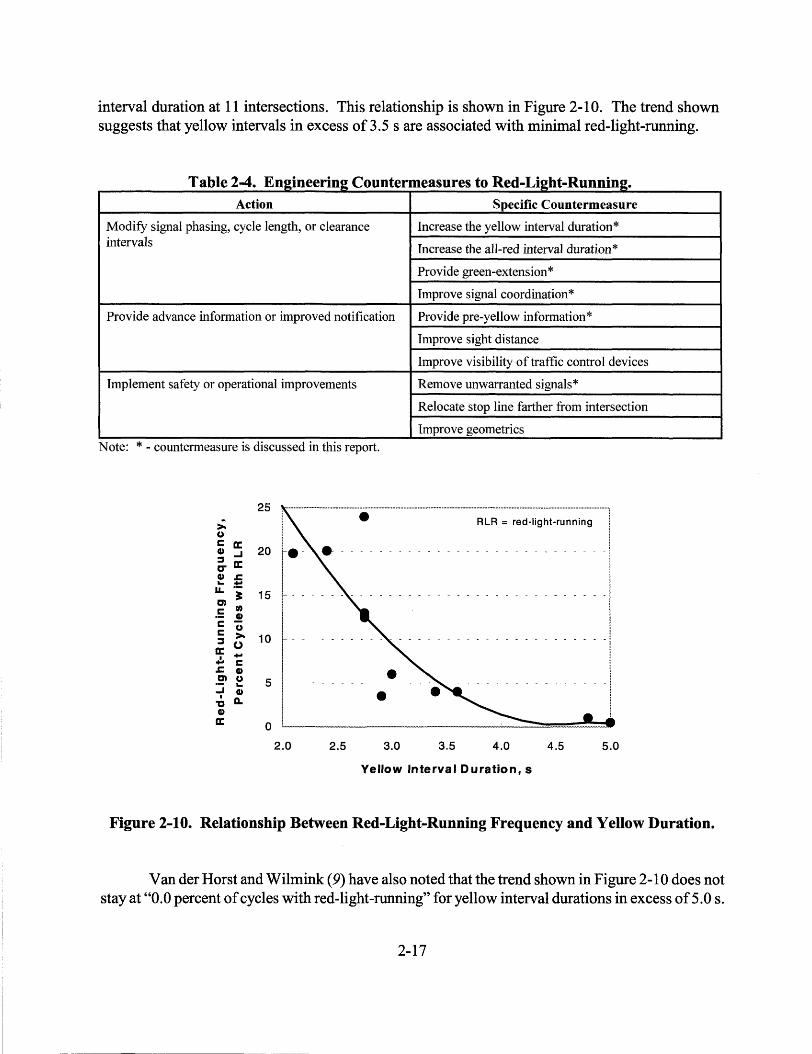
interval duration at 11 intersections. This relationship is shown in Figure 2-10. The trend shown suggests that yellow intervals in excess of 3.5 s are associated with minimal red-light-running.

T bl 2-4 E a e . nizmeerm2 c t oun ermeasures t Rd L" ht R 0 e - 12 - unmn2. Action Specific Countermeasure

Modify signal phasing, cycle length, or clearance Increase the yellow interval duration* intervals Increase the all-red interval duration*

Provide green-extension*

Improve signal coordination*

Provide advance information or improved notification Provide pre-yellow information*

Improve sight distance

Improve visibility of traffic control devices

Implement safety or operational improvements Remove unwarranted signals*

Relocate stop line farther from intersection

Improve geometrics Note: * - countermeasure is discussed in this report.

25 ................................................................................................................................. ~ ............................................................................................. "!

>­u ; 5 20 :I ~ C" G) .c ..... IL ·-m ;= c "' ·- .!

15

c u § ti 10 Cf .. .. c .c G) m u ·- ... ..I G)

,; Q. G)

~

5

0

2.0 2.5

•

• 3.0

i RLR = red-light-running

~ - - - - - - - - - - - - - - - - -t

; !

-I ! ! .................. !

3.5 4.0 4.5 5.0

Yellow Interval Duration, s

Figure 2-10. Relationship Between Red-Light-Running Frequency and Yellow Duration.

Van der Horst and Wilmink (9) have also noted that the trend shown in Figure 2-10 does not stay at "0.0 percent of cycles with red-light-running" for yellow interval durations in excess of 5.0 s.

2-17

Specifically, they note that there are " ... changes in drivers' behavior ... " for overly long yellow warning intervals. Presumably, the change is an increase in the frequency ofred-light-running with increasing yellow duration beyond 5. 0 s.

Increase the All-Red Interval Duration

Retting and Greene (23) examined the effect of all-red interval duration on the frequency of red-light-running. They found that increasing the all-red interval did not reduce the frequency of red­light-running. However, Hagenauer et al. (24) found that the addition of a nominal all-red interval did reduce the frequency of right-angle crashes by about 40 percent.

Provide Green-Extension

Green-extension is a countermeasure used at intersections with actuated control. It employs advance detectors on the major-road approaches. The detector placement and controller settings are designed such that a lengthy gap in traffic is needed before the phase is allowed to terminate. This scheme ensures that the approach is effectively clear of vehicles when yellow is presented unless the phase is forced to end because it has reached its maximum duration (i.e., it maxes-out).

Zegeer and Deen (I 0) and Baguley ( 8) have found that this scheme has the potential to reduce the frequency of red-light-running. However, each reports that the reduction is modest and highly dependent on the frequency of phase max-out. Baguley also noted that green-extension appeared to have the greatest positive effect for low-to-moderate volumes (i.e., a major-road volume less than 30,000 veh/day) and high speeds (i.e., greater than 55 mph).

Provide Pre-Yellow Information

Several kinds of control information have been used to supplement the yellow indication by giving drivers an advance warning of the impending change in right-of-way. The schemes used include:

• advance active warning signs, • flashing green indication prior to solid yellow indication, and • use of solid yellow concurrent with solid green prior to just solid yellow indication.

Farraher et al. (25) studied Minnesota Department of Transportation's (DOT) use of active advance warning signs at selected high-speed (50 mph or more) isolated intersections. Two "Be Prepared to Stop When Flashing" warning signs each combined with two 8-inch, flashing yellow beacons are located about 9 .5 s upstream from the intersection. The beacons flash for the last few seconds of the green and throughout the yellow and red indications. Measurements indicate that the system reduces red-light-running by 29 percent. However, Minnesota DOT recognizes that widespread deployment of this device may reduce this level of effectiveness.

2-18

Mahalel and Prashker (19) studied the effect of using a flashing green indication as an advance warning of phase change. The flashing green occurred for the last 3 s of the green interval; it was followed by a 3-s yellow interval. They found that the flashing green increased the zone of indecision (as noted in a previous section) and reduced the probability of stopping at any given location on the approach. Mahal el and Prashk:er also found that rear-end crash rates increased when flashing green was used.

Remove Unwarranted Signals

Traffic signals at intersections with low side-street volumes may contribute to red-light­running. Retting et al. ( 1) cite two studies that have found crashes to be reduced by about 24 percent through the removal of unneeded signals.

Improve Signal Coordination

Drivers approaching the intersection while the green is displayed and while traveling within a platoon are likely to expect that the indication will remain green at least until they pass through the intersection. This expectation was noted by Van der Horst and Wilmink (9). If the expectation is met through good coordination and wide progression bands (via long cycle lengths), red-light­running may be reduced; however, there does not appear to be any research to support this hypothesis.

Enforcement Countermeasures

Enforcement countermeasures require the use of police presence or some type of automated monitoring system. Police presence has been shown to have a significant short-term effect but is costly to sustain and any ensuing police chases may present a danger to bystanders. Automated enforcement typically uses a camera located on the intersection approach and connected electronically to the signal controller. A recent review of the effectiveness of such camera systems by Retting et al. (J) indicates that they have the potential to reduce right-angle crashes by 32 to 42 percent. One drawback of automated systems is that they cannot be used to identify the off ending driver-just the vehicle. The legal implications of this characteristic have prevented some states from using automated systems. More importantly, survey results reported by Retting et al. indicate that almost one-third of the U.S. drivers are strongly opposed to the use of automated systems.

2-19

CHAPTER 3. DATA COLLECTION PLAN

OVERVIEW

This chapter summarizes the development of a plan for collecting the data needed to quantify: (1) the effect of various factors on red-light-running frequency and (2) the effect ofred-light-running on right-angle crashes. Initially, a model of the red-light-running process is developed and described. This model is used to mathematically describe the events that lead to red-light-running and to define several useful measures of effectiveness. Next, countermeasures to red-light-running are evaluated and the most promising ones are identified. Finally, a comprehensive data collection plan is described.

MODEL DEVELOPMENT

Measures of Effectiveness

A review of the literature indicates that several measures quantify driver behavior at the end of a signal phase. The more commonly used measures include: "Percent of cycles with one or more red-light-runners," "Hourlyred-light-runningrate," and "Percent of vehicles thatrun the red." Other measures related to red-light-running and its consequences also exist, many of which are listed in Table 3-1.

T bl 3 1 R d L" ht R RI t dM a e - . e - If! - unnm2- eae easures o f Efti ti ec veness. lncident1 Frequency-based Measure Rate Location

Expressions 2' 3

Entry dur~g yellow 1. Vehicles entering during the yellow interval ... per hour ... per lane interval

2. Cycles with one or more entries on yellow ... per cycle ... per approach ... per vehicle ... per intersection

Entry during red 3. Vehicles entering during the red interval interval (RLR)

4. Cycles with one or more entries on red

5. Vehicles in intersection after end of all-red

Conflict due to RLR 6. Vehicle-vehicle conflict

Notes: 1 - RLR =red-light-running 2 - "per vehicle" relates to the total number of vehicles counted for the subject location. 3 - If the numerator and denominator have common units (e.g., cycles with one or more entries per cycle), then the ratio

is often multiplied by 100 and expressed as a percentage.

The second column in Table 3-1 lists the frequency-based measures that can be used to quantify problems related to red-light-running. Each of these measures can be converted into a rate­based measure by dividing the frequency measure by a "normalizing" factor. Three typical

3-1

normalizing factors are listed in Column 3 of Table 3-1. For example, the third frequency-based measure listed can be reported as a rate in terms of "vehicles running the red per hour," "vehicles running the red per cycle," or "vehicles running the red per total vehicles." These three rates can be quantified for a given lane, approach, or for the overall intersection.

"Entries during the yellow interval" and "conflicts due to red-light-running" are listed in Table 3-1 because they also provide some measure of driver behavior at the end of the phase. The former provides information about the driver's propensity to enter the intersection after the yellow is presented. Logically, large rates for this measure would correlate with large red-light-running rates. The conflict rate is also a useful measure as it combines the behavior of drivers on the subject approach with those on the conflicting approaches. Of those listed, this measure is likely to have the best correlation with the red-light-running-related crash rate.

The normalizing factors in Table 3-1 can also be referred to as "exposure" variables. They are not considered to be the direct cause of an event; however, there is inherently a linear relationship between the frequency of an event and the amount of exposure it receives. The slope of this line is referred to as the event rate.

Red-Light-Running Model

Model Development

This section describes the development of a model for predi<;;ting the frequency of red-light­running. The model is based on the probability of a driver stopping following the onset of the yellow indication when that driver is t seconds travel time from the stop line. This probability reflects the decision of each driver that decides not to stop as well as the first driver that decides to stop. It is represented mathematically as a probability distribution due to differences among drivers. Chapter 2 describes the effect of speed and other factors (e.g., grade, yellow interval duration, etc.) on the shape and orientation of this distribution.

Different probability distributions have been used to represent the probability-of-stopping relationship. Sheffi and Mahmassani (15) used the normal distribution. Bonneson et al. (16) used the logistic distribution. They selected the logistic distribution because its cumulative form exists as a closed-form equation form whereas that for the normal distribution requires a cumbersome integration. The logistic distribution is represented by the following equation:

1 p stop = 1 + e (a - t)IP (1)

where: p stop = probability of stopping in response to the yellow indication when at a given travel time t;

t = travel time to the stop line at the onset of yellow, s;

3-2

a = shift parameter (equals the travel time at which the probability of stopping is 0.5), s; and P = shape parameter, s-1

•

The complement to the probability of stopping is the "probability of going." This latter probability can be computed as:

P - 1 - p go stop (2)

where, Pgo =probability of going in response to a yellow indication when at a given travel time t. The probability of going is illustrated in Figure 3-1 as it relates to travel time .

... Cl) tn c 0 Yellow ;: 1 ..2 G) > ... ca CJ) c ·s " .... 0 >i

.:!:::::

:a ca

.Q 0 ... 0 Q.

0 5 Travel Time, s

1f L------------~----------~------

0 Travel Distance, ft 300

Figure 3-1. Probability of Going at Yellow Onset.

Shown at the bottom of Figure 3-1 is a schematic of an intersection approach with two vehicles. The travel time and travel distance axes are related by the approach speed. The two

3-3

vehicles are shown by their locations at the onset of the yellow indication. The probability curve in Figure 3-1 indicates that the driver nearest the stop line has a 75 percent chance of going. If this driver should choose to go, he or she will legally enter the intersection during the yellow indication. In contrast, the more distant driver has a 5 percent chance of going. If this more distant driver should go, he or she will run the red light as the yellow interval is shorter than his or her travel time to the intersection.

The red-light-running model is based on the development of a mathematical relationship that combines the first five events listed in Table 2-1 and the concepts shown in Figure 3-1. The form of this model is:

E[R] = Px m f Pgo q(t) dt y

where, E[R] = expected red-light-running frequency, veh/h;

p x = probability of phase termination by max-out; m = number of signal cycles per hour(= 3,600/C), cycles/hr; C = cycle length, s; t = travel time to the stop line at the onset of yellow, s;

Y = yellow interval duration, s; and q(t) = flow rate t seconds travel time from the stop line at the onset of yellow, veh/s.

(3)

The integral in Equation 3 computes the expected number of vehicles running the red at the end of a pretimed signal phase (or an actuated phase that maxes-out) for a given intersection approach. The two terms in the integral represent the number of vehicles at a given time t from the stop line (i.e., q(t) dt) and the probability of these vehicles "going" (i.e.,pg0 ). The integral sums all such possible events for the approach. A second integration over the distribution of approach speeds could be added if the probability of going is found to be a function of vehicle speed.

It should be noted that separate probability distributions may exist for each traffic movement on an approach (i.e., left-tum, through, right-tum), especially when the movement is allocated an exclusive lane (or lanes). If so, each movement should be evaluated with separate applications of Equation 3 and the values obtained added together to yield the total expected red-light-running frequency for the approach. However, to simplify the discussion in this report, the through movement is the subject of the discussion and evaluation. In this regard, it was assumed that the subject "approach" consists only of through vehicles.

Two assumptions are made to simplify Equation 3. First, it is assumed that the intersection is in an urban area such that the subject phase is pretimed (or it is actuated but maxes-out each cycle). This assumption results in the variable Px having a value of 1.0. Second, it is assumed that

3-4

q(t) is equal to the average approach flow rate q (i.e., q(t) = q). Based on these assumptions, Equation 3 simplifies to:

E[R] Qp C r

with,

where, Q = average approach flow rate(= q x 3600), veh/h; and Pr = propensity, s.

(4)

(5)

In Equation 5, the integral represents the propensity of drivers on the subject approach to "run the red light." This integral reflects the shaded area under the curve in Figure 3-1. It should also be noted that integration of Equation 5 from 0.0 to infinity 00 yields a value of Pr that equals the shift parameter a in Equation 1. When this parameter is multiplied by the flow-to-cycle-length ratio Q/C, the result is the expected number of vehicles going through the intersection during the yellow or red intervals.

Two of the more commonly used measures of effectiveness in the literature are "percent of vehicles running the red" and "percent of cycles with one or more red-light-runners." Both of these measures can be computed (and related to) Equation 4. For example, the "percent of vehicles running the red" P V.RLR on a given intersection approach can be computed as:

PV,RLR = 100 E[R]

Q p

100 _r

c

This measure is not influenced by the number of approach lanes.

(6)

If it is assumed that, for a given lane, only one vehicle runs the red per cycle when there is a red-light-runner, then the "percent of cycles with one or more red-light-runners"P c.RLR on an approach can be computed as:

3-5

PC,RLR 100 [1 - ( 1 - E~]r l 100 [ 1 _ ( 1 _ ~ pr l

where, n = the number of approach lanes.

(7)

The most important point to this discussion is that "propensity'' Pr is the most fundamental measure of the likelihood ofred-light-running on a given intersection approach. An examination of factors that influence red-light-running (e.g., speed, grade, yellow interval duration, etc.) should be focused on the effect of these factors on Pr. All other red-light-running measures represent some combination of the propensity variable and one or more exposure variables.

Model Calibration

The red-light-running model is represented by Equation 4, as supplemented by Equations 1, 2, and 5. Calibration of this model consists of quantifying the shift and shape parameters (i.e., a and ~)in Equation 1. This calibration can be achieved by either of two methods. Both methods require measurement of the cycle length and the approach flow rate.

One method requires direct measurement of the probability of stopping on an intersection approach. This method is quite complicated as it requires measurement of the speed, distance-to-the­stop-line, and the stop/ go decision for each vehicle on the intersection approach at the onset of yellow. Logistic regression is then used to calibrate the parameters in Equation 1.

A second method is based on a direct calibration of the red-light-running model (i.e., Equation 4). This method requires counting the number of drivers "going" during the red (i.e., running the red). This count is then compared with values predicted by Equation 4 using a nonlinear regression technique. This technique iteratively searches for the shape parameters that achieve the best overall fit. This calibration method is attractive because it requires only the measurement of the vehicles running the red.

COUNTERMEASURES TO BE EVALUATED

Based on a review of the countermeasures listed in Table 2-4 and discussions with engineers in Texas, it was determined that three countermeasures would be most appropriate for further study. These countermeasures are:

3-6

• increase the yellow interval duration, • improve signal coordination, and • improve visibility of traffic control devices.

For various reasons, the seven remaining countermeasures listed in Table 2-4 were not selected. For example, the literature review indicated that increasing the all-red interval was likely to reduce the frequency of right-angle crashes but not likely to reduce the frequency of red-light­running, which was the focus of this research. The literature review also indicated that pre-yellow information (e.g., flashing green indication for last few seconds of green) led to an increase in rear­end crashes, so this measure was ruled out.

Providing green-extension through advance detection was ruled out because this detection mode was more suitable for rural intersections (which is beyond the scope of this research project). "Improving sight distance to the intersection" and "improving intersection geometry" are viable countermeasures but their application would be very site-specific. Removal of unwarranted signals is also a viable countermeasure but represents a small subset of all problem intersections. Finally, relocation of the stop line to a point further back from the intersection was ruled out because of concerns that doing so might compromise sight lines and, in fact, increase the frequency of right­angle crashes.

SITE SELECTION AND DATA COLLECTION PROCEDURES

This section describes the development of a plan for collecting the data needed to calibrate the red-light-running model and to assess the effect of red-light-running on crash frequency. Initially, the site selection criteria are defined. Then, the candidate study sites are described. Finally, the data collection methods are outlined.

The data collection plan represents a hybrid design that combines both a cross-section study and a before-and-after study. The cross-section study is conducted first and is the focus of this section. The objective of this study is to quantify the effect of various factors (e.g., area population, speed, grade, yellow duration) on the frequency of red-light-running. This objective was achieved by identifying a set of study sites that collectively offer a range in each of the aforementioned factors.

The before-and-after study will follow the cross-section study. This study will take place during the second year of research. For this study, the three countermeasures identified in the previous section will be implemented at a subset of the study sites previously studied. The cross­section study previously conducted will serve as the "before" study. Those sites for which a countermeasure is not implemented will be used as a control site. The "after" study period will take place no sooner than two (and preferably six) months after implementation of the countermeasure. This approach will facilitate the examination of a countermeasure's long-term effect on the frequency of red-light-running. More details on the "before-and-after" study plan will be provided at the conclusion of Task 7 of the research project.

3-7

Site Selection Criteria

This section describes the criteria used to select the candidate study sites. Preliminary analysis indicated that a minimum of 10 study sites would be needed to provide the necessary data. A "study site" is defined to be one signalized intersection approach. The criteria used for site selection included the following items:

• Collectively, the study sites should reflect a range of yellow and all-red interval durations. • Collectively, the study sites should represent small, medium, and large Texas cities. • Collectively, the study sites should represent approach grades from -5 to + 1 percent. • Collectively, the study sites should represent speed limits from 30 to 50 mph. • Pavement markings should be clearly visible. • Approaching drivers should have a clear view of the signal heads for 7-s travel time. • Intersection should be in an urban or suburban area. • Crash history for the previous three years should be available. • Intersection skew angle should be less than 5 degrees. • There should be a minimum approach volume of 400 veh/hr/lane during the peak hour. • Pretimed control should be in use or, if actuated control is in use, the phase should frequently

terminate by max-out.

It was also recognized that these criteria were goals rather than objectives as it was not likely that all the criteria could be satisfied by each site given the time and resources available for the selection process.

Candidate Study Sites

The candidate study sites were identified through a series of activities. Initially, the research team solicited the names of potential study sites from the members of the project monitoring committee. This solicitation was followed by telephone contacts with the traffic engineers in several Texas cities. Finally, the research team added the names of several potential study sites that were believed to satisfy the selection criteria.

The research team visited each potential study site and made measurements of its physical size and traffic control characteristics. For each study site, a traffic engineer with the agency responsible for the site was contacted to solicit his or her interest in participating in the study. Finally, the attributes of the candidate study sites were reviewed and 12 study sites were selected. These sites represent six intersections in three Texas cities. The characteristics of each intersection are listed in Table 3-2.

3-8

Table 3-2. Intersection Characteristics. Characteristics

City Intersection1

Study Sites2 Cycle Advance Enforcement (Approach) Length3

, s Detection Lights?

Mexia Bailey St. (F.M. 1365) & Milam St (U.S. 84) EB,WB 75 No No

S.H. 14 & Tehuacana Hwy (S.H. 171) EB,WB 55 No No

College Texas Ave. (S.H. 6) & G. Bush Dr. (F.M. 2347) NB,SB 110 No No Station

College Main & University Dr. (F.M. 60) EB,WB 110 No No

Richardson Plano Road & Belt Line Road SB,EB 80-109 No Yes

Greenville Ave. & Main Street SB,EB 80-109 No Yes

Notes: 1 - North-south street is listed first. 2 - NB: northbound; SB: southbound; EB: eastbound; WB: westbound. 3 - Cycle lengths shown were observed during the site visit and may vary during the day.

The three cities included in the study collectively represent a wide range in population and facilitated the examination of "small town" versus "big city'' driver behavior. The city of Mexia has a population of 7 ,000 persons and the combined cities of Bryan/College Station have a population of 107 ,000. In contrast, the city of Richardson is in the Dallas/Fort Worth metropolitan area that has a population of about three million persons.

The City of Richardson has an active red-light-running enforcement program that uses white enforcement lights to help police officers determine the status of the red indication from a strategic position downstream from the intersection. It should be noted that this program has been in place for more than three years and its "novelty" effect was considered to be negligible. As such, it was believed to have no effect on the proposed study findings (enforcement activities were not in progress during any study).

At each intersection listed in Table 3-2, two intersection approaches were selected for a formal field study and an evaluation of its crash history. The candidate study site (i.e., intersection approach) characteristics are listed in Table 3-3. The data in this table indicate that the study sites collectively offer a reasonable range of speeds, grades, yellow interval durations, and signal head types.

3-9

a e - . an 1 ae u lY I e t . f arac eris 1cs. City Study Site Characteristics

Speed Grade, 1 Yellow Limit, mph O/o Interval, s

Mexia EB Milam St. 35 -2.8 3.9

WB Milam St. 35 +2.8 4.0

EB S.H. 171 30 -0.5 4.0

WB S.H. 171 30 0.0 4.0

College NB Texas Ave. 40 0.0 3.5 Station SB Texas Ave. 40 -0.5 3.5

EB University Dr. 35 +0.5 3.2

WB University Dr. 35 +0.2 3.2

Richardson SB Plano Road 40 +0.5 4.4

EB Belt Line Road 35 0.0 4.0

SB Greenville Ave. 30 +0.5 3.6

EB Main Street 30 0.0 3.7 Notes: I - Grade: plus ( +) grades are upgrades in a travel direction toward the intersection. 2 - Signal head type: all indications use bulb lighting, except as noted in the table.

All-Red Interval, s

1.0

1.0

1.0

1.0

1.0

2.0

1.0

1.0

2.0

2.5

2.0

2.0

Signal Head Type 2

Red: LED

Red: LED

bulb

bulb

bulb

bulb

bulb

bulb

bulb

bulb

bulb

bulb

Based on discussions with the traffic engineer responsible for the signalization at each study site, one countermeasure was selected for application. The proposed countermeasure for each site is identified in Table 3-4. The proposed countermeasures will be studied during the second year of the project.

Eight additional study sites were added to the 12 study sites listed in Tables 3-2, 3-3, and 3-4. These study sites were added after the studies were conducted at the original 12 study sites and at the request of the project director and the Project Monitoring Committee. The addition adds breadth to the collective set of study sites in terms of adding sites with higher speeds, steeper grades, or both. Information about the study sites and the results of the field studies at these locations will be incorporated in the database during the second year of the project.

3-10

T bl 3 4 P a e - . ropose dC t t E h St d S"t oun ermeasure a ac u ly I e. City Study Site Countermeasure

Mexia EB Milam St. Add LED lighting to all signal indications to improve visibility

WB Milam St. Add LED lighting to all signal indications to improve visibility

EB S.H. 171 Control site

WB S.H. 171 Control site

College Station NB Texas Ave. Increase yellow interval duration

SB Texas Ave. Control site

EB University Dr. Adjust signal progression and increase cycle length

WB University Dr. Adjust signal progression and increase cycle length

Richardson SB Plano Road Increase yellow interval duration

EB Belt Line Road Increase yellow interval duration

SB Greenville Ave. Increase yellow interval duration

EB Main Street Control site

Data Collection Procedure

The data collection plan consisted of two data collection activities. The first activity relates to the field study of the sites described in the preceding section. The second activity relates to the assembly of crash records for the three most-recent years at each study site. The types of data collected and the methods used to collect these data are described in the remainder of this section.

Field Data Collection

The field study of each site included the collection of a wide range of geometric, traffic flow, traffic control, and operational characteristics. These data were collected using a variety of methods including videotape recorders, laser speed guns, and site surveys. The data collected during each field study and the methods of collection are listed in Table 3-5.

During the study of each site, one videotape recorder was positioned upstream of the intersection such that its field-of-view included the appropriate signal heads and all lanes of the subject through movement. Typically, the recorder was located about 150 ft upstream of the subject stop line. The data were extracted from the videotape during its replay in the office. A sample of the vehicle speeds on the intersection approach in the subject lanes was also taken while the approach was being videotaped. Speeds were measured only for those vehicles unaffected by signal­related queues. This speed was intended to represent that of vehicles on the approach at the onset of the yellow indication.

3-11

Table 3-5. Database Elements. Data Collection Method

Category Data Type Reduced from Site Agency

Videotape Survey Files

Geometric Number and width of intersection traffic lanes .,. Characteristics

Distance to adjacent signalized intersections .,. Approach grade .,. Photo log .,.

Traffic Flow Traffic movement counts ti' Characteristics

Heavy-vehicle percentage ti'

Traffic Control Speed limit ti' Characteristics

Phase sequence .,. Yellow interval duration .,. All-red clearance interval duration .,.

Operational Cycle length ti' Characteristics

Average running speed .,. Count of yellow-light-runners ti'

Count of red-light-runners ti'

Safety Overall" crash frequency during past 3 years .,. Characteristics

Average daily traffic volume by leg ti'

Safety Data Collection

The safety data collection activity consisted of the acquisition ofhistorical crash records for each intersection included in the field studies. To facilitate the analysis, computerized databases were requested from the Texas Department of Public Safety and the appropriate city agencies. The request was for the most recent 36 months for which complete information was available and for all four approaches to each intersection. These data were used to quantify the relationship between red­light-running and crash frequency.

A traffic engineer at each agency responsible for a study intersection was also contacted to gather additional information needed for the crash data analysis. Specifically, inquiry was made regarding the history of the study site for the purpose of ruling out crash data during months (or years) during which the geometry or control mode were not consistent with that of the existing intersection. Also, the average daily traffic demand for each intersection leg was obtained during this contact.

3-12

CHAPTER4. DATAANALYSIS

OVERVIEW

This chapter summarizes an analysis of the causes and effects of red-light-running. Specifically, the analysis examined two issues: (1) the factors that lead to red-light-running, and (2) the effect ofred-light-running on right-angle crashes. The analysis of factors affecting red-light­running is based on the model described in Chapter 3. The analysis ofred-light-running's effect on crash frequency is based on an examination of the relationship between the crash rates and red-light­running rates at several intersections. Each of these two analyses is described in a separate section of this chapter.

FACTORS AFFECTING RED-LIGHT-RUNNING

This section describes the findings from an investigation of the factors that affect red-light­running. The findings presented are the result of a statistical analysis of a red-light-running database assembled for this research. Initially, the database content is summarized and reviewed for the existence of basic cause-and-effect relationships. Then, the Red-Light-Running Model calibration is discussed and the statistical approach used for this effort is described. Finally, this section concludes with a sensitivity analysis. This analysis illustrates several of the factors that have an effect on red-light-running.

Database Summary

The database assembled for this research includes the traffic, geometric, and control characteristics for six intersections in Texas. Two approaches were studied at each intersection. Traffic data recorded at each intersection included: traffic volume and vehicle classification for each signal cycle (passenger cars and heavy vehicles), cycle length, number ofred-light-running vehicles per cycle, average running speed, and flow rate at the end of the phase. Details of the site selection criteria and the geometric and control characteristics of each site are included in Chapter 3.

Summary statistics describing the database are provided in Tables 4-1and4-2. The ranges listed in Table 4-1 indicate that the study sites collectively offer good representation of typical yellow interval durations, all-red interval durations, and number of approach lanes. The range of values for grade and speed limit was not as broad as desired and does not reflect steep grades nor high speeds. Additional data collection is planned that will broaden the database and overcome these limitations.

The data in Table 4-2 indicate the number of observations of each traffic variable. With the exception of the running-speed data, the observations reflect six hours of data collection on each intersection approach. All total, more than 3, 100 signal cycles were observed at 12 intersection approaches. During these cycles, 189 vehicles entered the intersection after the change in signal indication from yellow to red.

4-1

T bl 4 1 D t b a e - . a a ase s ummary- G t . eome r1c an d T ffi C t l V . bl ra IC on ro aria es. Variable Statistic City Overall

Mexia I College Station I Richardson

Yellow Interval Minimum: 3.9 3.2 3.6 3.2 Duration, s Maximum: 4.0 3.5 4.4 4.4

All-Red Interval Minimum: 1.0 1.0 2.0 1.0 Duration, s Maximum: 1.0 2.0 2.5 2.5

Grade,% Minimum: -2.8 -0.5 0.0 -2.8

Maximum: 2.8 0.5 0.5 2.8

Number of Minimum: 1 3 2 1 Approach Lanes Maximum: 2 3 3 3

Speed Limit, Minimum: 30 35 30 30 mph Maximum: 35 40 40 40

T bl 4 2 D t b s T t lOb f a e - . a a ase ummary- oa serva ions. City Intersection Total Observations

Approach Vehicles Cycles Speeds Red-Light-Runs

Mexia EB Milam St. 2,531 285 100 13

WB Milam St. 2,728 288 100 9

EB S.H. 171 509 408 20 0

WB S.H. 171 1,073 412 36 1

College Station NB Texas Ave. 6,801 195 100 24

SB Texas Ave. 6,372 191 100 10

EB University Dr. 5,732 194 100 34

WB University Dr. 5,546 195 100 60

Richardson SB Plano Road 4,673 232 81 4

EB Belt Line Road 3,382 232 93 6

SB Greenville Ave. 1,764 236 41 3

EB Main Street 5,179 243 100 25

Total: 46,290 3,111 971 189

The running speeds were obtained during a spot speed survey conducted simultaneously with the collection of the other data listed. Speed data were collected after the queue had cleared following the start of each phase. These data included only vehicles moving at a speed consistent with the mid-block running speed. An analysis of speed variance indicated that 100 speed observations would yield an estimate of the mean running speed with a precision of± 1 mph or less with a 95 percent confidence level. Hence, the goal was to measure 100 speeds for each intersection

4-2

approach. Unfortunately, at a few locations, there was insufficient traffic volume to yield 100 observations of running speed during the six-hour study.

Table 4-3 lists the statistics associated with selected traffic characteristics included in the database. In general, these statistics indicate that there is a wide range of volume and cycle length in the database. The heavy-vehicle percentage also exhibits a reasonably wide range of values given that the intersections were all located within city limits.

T bl 4 3 D t b a e - . aa ase s ummary- St f ti fi S 1 t d V . bl a 1s cs or e ec e aria es. Variable Statistic1 City Overall

Mexia I College Station I Richardson

Approach Average: 285 1018 625 643 Volume, veh/h Std. Deviation: 164 197 278 370

Minimum: 61 698 195 61

Maximum: 517 1384 1306 1384

Running Speed, Average: 34 37 35 35 mph Std. Deviation: 4.0 5.3 6.3 5.5

Minimum: 20 24 21 20

Maximum: 45 52 48 52

Observations: 256 400 315 971

Cycle Length, s Average: 63 110 92 88

Std. Deviation: 11 0 11 21

Minimum: 49 110 75 49

Maximum: 75 110 109 110

Heavy-Vehicle 2 Average: 6.4 2.4 3.5 4.1 Percentage, % Std. Deviation: 2.8 1.3 1.5 2.6

Minimum: 1.8 0.9 1.3 0.9

Maximum: 12.4 6.2 6.5 12.4

Phase-End Flow Average: 297 1452 981 910 Rate, veh/h Std. Deviation: 185 763 624 744

Minimum: 48 107 289 48

Maximum: 660 2609 2378 2609 Note: 1 - With the exception of Running Speed, all statistics are based on six observations of the subject variable-one

observation for each of the six study hours. Running speed statistics are based on the observation of individual vehicle speeds. The number of vehicles for which speed was measured is indicated in the row labeled Observations.

2 - A "heavy vehicle" is defined as any vehicle with more than four tires on the pavement, with the exception of a 1-ton pickup truck with dual tires on the rear axle (this truck was considered to be a "passenger car").

4-3

The "phase-end flow rate" listed in the last row of Table 4-3 represents the flow rate at the end of the phase. Observations during the field studies indicated that flow rates varied considerably during the signal cycles, often due to upstream signalization. At some intersections, the platoons of traffic created by these upstream signals would often arrive near the end of the phase. When this occurred, the propensity for red-light-running appeared to be higher than at intersections of similar volume but with random arrivals or with platoons arriving nearer to the start of green. A subsequent section discusses this effect of flow rate on red-light-running.

Statistical Approach for Model Calibration

A preliminary examination of the red-light-running data indicated that it is neither normally distributed nor of constant variance, as is assumed when using traditional least-squares regression. Under these conditions, the generalized linear modeling (GLIM) technique, described by McCullagh and Nelder (26), is often used because it accommodates explicit specification of the error distribution using maximum-likelihood principles. This technique has been applied to crash data by several researchers, including Hauer et al. (27) and Bonneson and McCoy (28). In fact, the latter researchers developed procedures for automating the GLIM technique using the SAS ® statistical analysis software (29).

Terminology

The distribution of red-light-running frequency can be described by the family of compound Poisson distributions. In this context, there are two different sourc~s of variability underlying the distribution. One source of variability stems from the differences in the mean red-running frequency m among the otherwise "similar" intersection approaches. The other source stems from the randomness in red-light-running frequency at any given site, which is most likely to follow the Poisson distribution.

In spite of being similar, each intersection approach in the group has its own regional character and driver population which give it its own unique mean red-light-running frequency, m;. Thus, the distribution of m's within the group of similar sites can be described by a probability density function with mean E(m) and variance V(m).

Abbess et al. (30) have shown that if event occurrence at a particular location is Poisson distributed then the distribution of events around the E(m) of a group of segments can be described by the negative binomial distribution. The variance of this distribution is:

E(m)2 V(x) = E(m) + --

k (8)

where, x is the observed red-light-running frequency for a given approach with an expected frequency of E(m). Recognizing that the variance of the Poisson distribution is E(m), it is apparent

4-4

that the variance of the negative binomial distribution exceeds that of the Poisson by the amount E(m}2!k.

The nonlinear regression procedure (NLIN) in the SAS software (29) was used to estimate the red-light-running model coefficients. This procedure is sufficiently general that it can be modified to accommodate error structures that are not normally distributed. It can also be modified to yield maximum-likelihood model coefficients. With these modifications, the NLIN procedure can be used as a generalized linear modeling tool.

Quality of Fit

Several statistics are available for assessing model fit and the significance of model coefficients. One measure of model fit provided by NLIN is the generalized Pearson i statistic. This statistic is calculated as:

i = L [x -!<m )]2 V(x)

(9)

where, V(x) is estimated from Equation 8 by substituting E(m) for E(m). This statistic is available from NLIN as the "Sum of Squares" for the residual. McCullagh and Nelder (26) indicate that this statistic follows the i distribution with n-p-1 degrees of freedom where n is the number of observations and p is the number of model parameters. This statistic is asymptotic to the x2

distribution for larger sample sizes and exact for normally distributed error structures. As noted by McCullagh and Nelder, this statistic is not well-defined in terms of minimum sample size when applied to non-normal distributions; therefore, it probably should not be used as an absolute measure of model significance.

Another, more subjective, measure of model fit can be obtained from a graphical plot of the prediction ratio versus the estimate of the expected red-light-running frequency (i.e.,E(m) ). In this context, the prediction ratio is defined as the normalized residual (i.e., the difference between the predicted and observed red-light-running frequencies divided by the standard deviation, J"V(x)). This type of plot yields a visual assessment of the predictive capability of the model over the full range of E(m). A well-fitting model would have the prediction ratios symmetrically centered around zero over the range of E(m), with almost all ratios falling between -3.0 and 3.0.

The significance of the parameter coefficients (with respect to the hypothesis that they equal zero) is also helpful in assessing the relevance of model factors. In this regard, NLIN provides the standard error and 95 percent confidence interval for each coefficient. Because the Pearson x2

statistic (i.e., Equation 9) has some limitations, the significance of the individual parameter coefficients may represent a more realistic measure of model fit.

A third measure of fit is the dispersion parameter crd. This parameter was noted by McCullagh and Nelder (26) to be a useful statistic for assessing the amount of variation in the

4-5

observed data. This statistic can be calculated by dividing Equation 9 by the quantity n-p. It is also available from NLIN as the "Mean Square" for the Residual. A dispersion parameter near 1.0 indicates that the assumed error structure is approximately equivalent to that found in the data. For example, if a Poisson error structure is assumed (i.e., V(x) = E(m)) and the dispersion parameter is 1.68, then the data have greater dispersion than is explained by the Poisson distribution. In this situation, the negative binomial distribution should be considered as it has a larger variance than the Poisson (see Equation 8).

Finally, the coefficient of determination R2 can be used to assess the quality of model fit. This statistic is commonly used for normally distributed residuals; hence, it loses some of its meaning when applied to non-normal residuals. Nevertheless, K valseth ( 31) has investigated the use of R2 to evaluate model forms calibrated with data having non-normal error structures and concluded that it can still be a useful tool if computed with the following equations:

R 2 = l _ SSE SST

with,

n

SSE = L (Yp,i - Ya)2

i

n

SST= L (Yo,i - Ym)2

i

where: y 0, i = observed dependent value for a given set of independent variables i; Yp, i = predicted dependent value for the same set of independent variables i; and y m = mean of all n observed dependent values.

(10)

(11)

(12)

When applied to the prediction of red-light-running frequency, the quantity obtained from Equation 10 is not a true R2 value because the residuals are not necessarily independent, normally distributed variates with constant variance. Nevertheless, it can also be loosely compared to traditional R2 values with similar interpretation.

Database Review and Analysis

Preliminary Review of Red-Light-Running Data

As a practical first step in the analysis of the data, red-light-running rates were computed for each intersection approach. Two rates were computed. The first rate is expressed in terms of red-

4-6

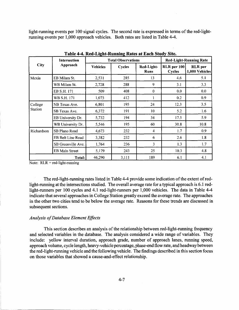
light-running events per 100 signal cycles. The second rate is expressed in terms of the red-light­running events per 1,000 approach vehicles. Both rates are listed in Table 4-4.

T bl 4-4 R d L. ht R a e . e - 1g - unmng R t t E h St d s·t a es a ac U IY I e. Intersection Total Observations Red-Light-Running Rate

City Approach Vehicles Cycles Red-Light- RLRper 100 RLRper Runs Cycles 1,000 Vehicles

Mexia EB Milam St. 2,531 285 13 4.6 5.1

WB Milam St. 2,728 288 9 3.1 3.3

EB S.H. 171 509 408 0 0.0 0.0

WB S.H. 171 1,073 412 1 0.2 0.9

College NB Texas Ave. 6,801 195 24 12.3 3.5 Station SB Texas Ave. 6,372 191 10 5.2 1.6

EB University Dr. 5,732 194 34 17.5 5.9

WB University Dr. 5,546 195 60 30.8 10.8

Richardson SB Plano Road 4,673 232 4 1.7 0.9

EB Belt Line Road 3,382 232 6 2.6 1.8

SB Greenville Ave. 1,764 236 3 1.3 1.7

EB Main S.treet 5,179 243 25 10.3 4.8

Total: 46,290 3,111 189 6.1 4.1

Note: RLR =red-light-running

The red-light-running rates listed in Table 4-4 provide some indication of the extent ofred­light-running at the intersections studied. The overall average rate for a typical approach is 6.1 red­light-runners per 100 cycles and 4.1 red-light-runners per 1,000 vehicles. The data in Table 4-4 indicate that several approaches in College Station greatly exceed the average rate. The approaches in the other two cities tend to be below the average rate. Reasons for these trends are discussed in subsequent sections.

Analysis of Database Element Effects

This section describes an analysis of the relationship between red-light-running frequency and selected variables in the database. The analysis considered a wide range of variables. They include: yellow interval duration, approach grade, number of approach lanes, running speed, approach volume, cycle length, heavy-vehicle percentage, phase-end flow rate, and headway between the red-light-running vehicle and the following vehicle. The findings described in this section focus on those variables that showed a cause-and-effect relationship.

4-7

The effect of approach volume on red-light-running frequency is illustrated in Figure 4-1. This figure indicates that red-light-running frequency increases with increasing volume. The volume reported in this figure represents an average volume and was computed as the total number of vehicles observed during one hour. It should be noted that in this and subsequent figures, each data point represents one hour of data from one intersection approach (a total of 72 ( = 12 * 6) data points are shown).

16 tn .E 14 c c

- - - - - - - - - - - - - - - - - - - -00 - - - - - - - - - -R2 = 0.31 0

:J :E 12 a: I .c - Q) .c > 10

.2> >-..J I u 8

"C c Q) Q)

a: :J 6 C" "C Q) Q) ...

4 > IL ... Q) fl) 2 .D 0

0

0 200 400 600 800 1 ,000 1 ,200 1 ,400

Approach Volume, veh/h

Figure 4-1. Red-Light-Running Frequency as a Function of Approach Volume.

Figure 4-2 presents a comparison of the relationship between phase-end flow rate and red­light-running frequency. Like that found for approach volume, red-light-running frequency increases with increasing flow rate. However, the degree of correlation (i.e., R2

) associated with phase-end flow rate is more than twice that found for approach volume. The significance of this improvement in fit suggests that any prediction of red-light-running frequency should be based on phase-end flow rate.

As noted in a previous section, the flow rate at the end of the phase is likely to be more intense in signalized street systems, particularly when the end of the platoon arrives to the approach at the end of the signal phase. In this situation, it is logical that more drivers are repetitively put in the position of having to decide whether to stop at the onset of yellow, relative to an isolated intersection or one where a larger majority of platoon drivers arrive at the start of green.

4-8

16 D)

.5 14 c c ::::s .c 12 'F :c ~ ~ 10 .!!> >. -7 u 8 'a c CD CD a: ::::s 6 'a CT CD ~ ~ lL 4 CD UJ .a 2 0

0

0

- - - - - - - - - - - - - - - - - - - - - - - - - - - - - - - -0 R

2 = 0.63 0

- - - - - - - - - - - - - - - - - - - - - - - -0- - - - - -0-0

- - - - - - - - - - - - - - - - -0- - - - - - - -0- - -0

- - - - - - - - - - -0- - - - - - - - - - - - - - - - - - -0

- - - -0- - - - - - - - - -0 0 0

- - - 0 CIDCD - - - - -0 - - - - - - - - - - - - 0- - - - -0 ()([) ClID (X)

500 1,000 1,500 2,000 2,500

Phase-End Flow Rate (Q 8 ), veh/h

Figure 4-2. Red-Light-Running Frequency as a Function of Phase-End Flow Rate.

Figure 4-3 illustrates the relationship between yellow interval duration and red-light-running frequency. The best-fit trend line shown suggests a curved relationship where yellow intervals in excess of 4.0 s are associated with less than 1.0 red-light-running vehicle per hour. This trend is very consistent with that reported by Van der Horst and Wilmink (9) (see Figure 2-10). It suggests that yellow interval durations ofless than 3.5 s may result in frequent red-light-running, even though they may be consistent with recognized practices regarding the determination of yellow interval duration (see, for example, Reference 32).

Figure 4-4 illustrates the relationship between heavy-vehicle percentage and red-light-running frequency for two of the three cities. A similar relationship was not found in the data from the Richardson sites. In general, the trends shown suggest that red-light-running frequency increases with heavy-vehicle percentage. An examination of the cause of this trend indicated that heavy vehicles are over-represented in the count of red-light-runners observed for this study. Specifically, heavy vehicles were found to represent 4.1 percent of all vehicles observed; however, they represented 6.4 percent of all red-light-running vehicles observed. A test of proportions indicated that this difference is significant at a 90 percent level of confidence (i.e., 10 percent chance of error).

4-9

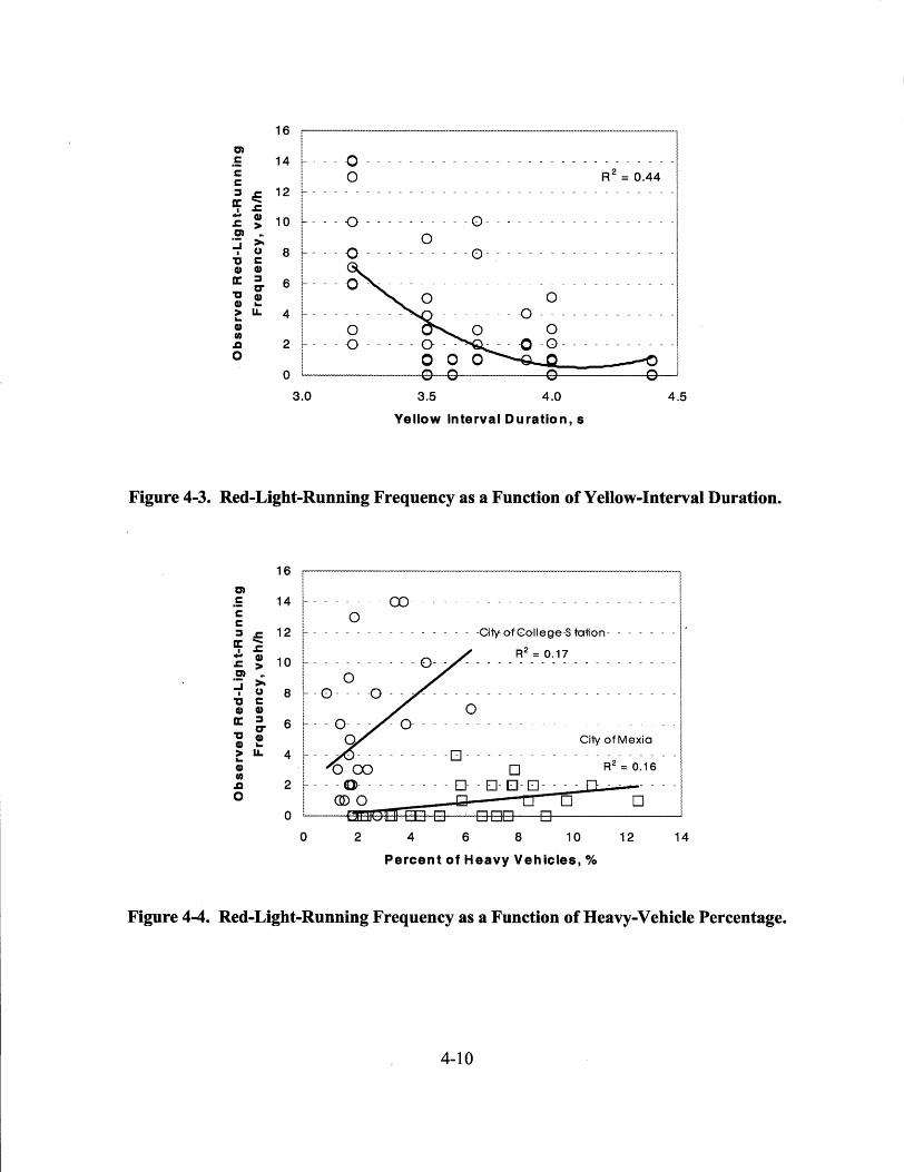
16 C)

·= 14 c c ::::J :E 12 a:

I .c

••• ~ •••••••••••••••••••••• R;=~ - CD 10 .c > - - - 0 - - - - - - - - - -0- - - - - - - - - - - - - - - - - -.2> >-..J

I u 8 "O c

0 - - - 0 - - - - - - - - - -o- - - - - - - - - - - - - - - - - -

CD CD a: ::::J 6 er "O CD CD ...

- - -o- ---- - - -- ------ -- -- - ---- --- - -0 0

> IL 4 ... - - - - - - - -0 - - - - - - - - - - - - -CD 0 .Q 2 0

0

---g -----o - - _o_ - - -o _g_ - - - - - - - - - -1

0 0 0 0 0 0 0

3.0 3.5 4.0 4.5

Yellow Interval Duration, s

Figure 4-3. Red-Light-Running Frequency as a Function of Yellow-Interval Duration.

16 ~, ~~~~~~~~~~~~~~~~~~~--, ;

C)

·= c c ::::J .c a: ......

I .c - CD .c > .2> >-..J

I u "O c CD CD

14 r · · · ·o · · CD · · · · · · · · · · · · · · · · · · · · · · · ·

12 ~ - - - - - - - - - - - - - - - -City- ofCollege-S tation- - - - - - - ! ·

l R2 = 0.17 10 ~ - - - - - - - - - - 0- - - - - - - - - - - - - - - - - - - - - -

! 0 I

8 ~ - 0- - - -0 - - - - - - - - - - - - - - - - - - - - - - - - - - -I o

a: ::::J

"O er CD

CD ... > IL ... CD 0 .Q

0

6 ~ - - 0- - - - 0- - - - - - - - - - - - - - - - - - - - - - - - -I a Ci1y of Mexia

4 ~ - - - - - - - - - - - - -[] - - - - - - - - - - - - - - - - - - - -I 0 (X) D R

2 = 0.16

2 ~ - - - 0- - - - - - - - - D- - EJ- EJ- D- - - - 0 - -I CIDO i;J D D D

o : lit]Q[] EE D DOD D 0 2 4 6 8 10 12 14

Percent of Heavy Vehicles,%

Figure 4-4. Red-Light-Running Frequency as a Function of Heavy-Vehicle Percentage.

4-10

Model Calibration

The findings from the preliminary review and analysis were used to develop the final form of the red-light-running model. The basic form of this model was previously described in Chapter 3; it is repeated below in the form used in the regression analysis:

with,

where, E[R]=

Qe= C= Y=

E[R] ~ ~ f [1 _ (1 + e (lineartermsl) i J dt y

expected red-light-running frequency, veh/h; phase-end flow rate, veh/h; cycle length, s; yellow interval duration, s;

t = travel time to the stop line at the onset of yellow, s; selected traffic and geometric characteristics; and regression coefficients, i = 0, 1, 2, ... , n.

x.= I

b= I

(13)

(14)

A wide range of variables was considered in the regression analysis. These variables include: yellow interval duration, approach grade, number of approach lanes, running speed, approach volume, cycle length, heavy-vehicle percentage, phase-end flow rate, and headway between the red­light-running vehicle and the following vehicle. Each variable was individually included in the model and, if found to be significant, allowed to remain.

The regression analysis revealed that mathematic relationships existed between red-light­running frequency and heavy-vehicle percentage, following headway, and grade. However, only heavy-vehicle percentage was found to be significant at a level of confidence that exceeded 90 percent. This finding suggests that additional data are needed to confirm whether the other variables truly affect red-light-running frequency, as suggested by the existing data. As a result of this analysis, the "linear terms" component of the model was specified as:

where,

HV linear terms = b0 - b1 t + b2 -100

HV = percent of heavy vehicles in the traffic stream.

4-11

(15)

It should be noted that a "heavy vehicle" is defined as any vehicle with more than four tires on the pavement, with the exception ofa 1-ton pickup truck with dual tires on the rear axle (this truck was considered to be a "passenger car").

The statistics related to the calibrated red-light-running model are shown in Table 4-5. The calibrated coefficient values would be used with Equations 13 and 15 to predict the hourly red-light­running frequency for a given intersection approach. A kparameter of 3.8 was found to yield the desired dispersion parameter of 1.0. The Pearson x2 statistic for the model is 69 and the degrees of freedom are 68 (= n-p-1 =72-3-1). As this statistic is less than i 0 05 68 = 89, the hypothesis that the model fits the data cannot be rejected. The R2 for the model is 0. 73: As this value is relatively large, it is reasoned that the model yields a good fit to the data.

With one exception, the coefficients in this model are significant at a 95 percent level of confidence. The coefficient associated with heavy-vehicle percentage is significant at the 90 percent level, which indicates that there is a 10 percent chance that the effect is truly nonexistent. However, this percentage is still acceptably small and likely due to variation among study sites (see Figure 4-4 ).

T bl 4 5 C l"b . t d R d L. ht R a e - . a 1 ra e e - 12 - unmn2 M d I St ft" ID o e a is 1ca "f escr1p ion. Model Statistics Value

R1: 0.73

Dispersion Parameter: 1.0

Pearson x2: 69.0 (x2 o.os, 68 = 89)

k Parameter: 3.8

Observations: 72 hours

Standard Error of an Individual Prediction: ±1.8 veh/h

Range of Model Variables

Variable Variable Name Units Minimum Maximum

Qe Phase-end flow rate veh/h 48 2,609

c Cycle length s 49 110

y Yellow interval duration s 3.2 4.4

HV Heavy-vehicle percentage % 0.9 12.4

Calibrated Coefficient Values

Variable Definition Value Std. Dev. t-statistic

ho Intercept 7.82 2.56 3.1

bl Effect of travel time to stop line 2.33 0.63 3.7

b2 Effect of heavy vehicles 11.64 6.78 1.7

4-12

The fit of the model was assessed using the prediction ratios plotted against the predicted accident frequency. The prediction ratio P Ri for intersection approach i represents its residual error standardized (i.e., divided) by the square root of its predicted variance (obtained from Equation 8). This ratio is computed as:

Yp,i - Yo,; (16)

The plot of prediction ratios for the study sites is provided in Figure 4-5. The trends shown in this figure indicate the model provides a good fit to the data. The prediction ratios have the desired feature of being centered around zero. This pattern indicates that there is no bias in the model predictions. The trend also indicates that the ratios are distributed normally about zero and within the range of ±3 .0 for the entire range of predicted values. This trend was the desired result; it is a consequence of the specification of the negative binomial error structure in the SAS NLIN procedure.

3.a

2.a 0 ;::;

"' a: 1.a c 0 ;::; -~ a.a "tJ G) ...

D..

-1.a

-2.a

l. 0

..... -0....... ......... I I 0 o 0 I ~ 0 -o - - - - - -o- - -o0o - - - - - - - - - - - - - - - - - - -I

I i % coo 0 0 ad ~' ·~ 0 .. 0. ~. . . . . . . ... 0. 0. 0 .

r---~---D-----0--------------------

1

a 2 4 6 8 10 12

Predicted Red-Light-Running Frequency, veh/h

Figure 4-5. Prediction Ratio versus Predicted Red-Light-Running Frequency.

A second means of visually assessing the model's fit is through the graphical comparison of the observed and predicted red-light-running frequencies. This comparison is provided in Figure 4-6. The trend line in this figure does not represent the line of best fit; rather, it is a "y = x" line. The data would fall on this line if the model predictions exactly equaled the observed data. The trends shown in this figure indicate that the model is able to predict the red-light-running without bias. The scatter

4-13

in the data suggests that there is still some unexplained systematic variability or some random variability in the data. In general, the model is able to predict the red-light-running frequency at a given site with a standard error of± 1.8 veh/h.

16 D)

·= 14 - - - - - - - - - - - - - - - - - - - - - - - - - - - - - - - -00 c c 0 ;:, .c 12 a: ......

I .c - Cl) 10 .c >

.2l >-..J I CJ 8

'tJ c Cl) Cl)

a: ;:, 6 er 'tJ Cl) Cl) ... > lL 4 ... Cl) tn

2 .D 0

0

0 2 4 6 8 10 12

Predicted Red-Light-Running Frequency, veh/h

Figure 4-6. Comparison of Observed and Predicted Red-Light-Running Frequency.

The calibrated model can be rewritten to yield the following form:

E[R] = ~ J [1 _ (1 + e (7 &2 -2331+0116HVJ)-1] dt y

(17)

Recognizing that the integral poses problems for practical application, an alternative form of the model was developed that is based on a tabular presentation of the integral values. The alternative form of the model is:

E[R] Qe p C r

(18)

where, Pr = propensity (see Table 4-6), s.

4-14

The values of the propensity variable are provided in Table 4-6 for a typical range of heavy­vehicle percentages and yellow interval durations. For example, if an intersection approach has a yellow interval duration of 4.0 sand has 5.0 percent heavy vehicles, the propensity Pr is 0.15 s. This value would then be used in Equation 18 to predict the hourly red-light-running frequency. The shift parameter (a) listed in Table 4-6 is included as a reminder of the meaning of the regression terms and their relationship to the probability of stopping (see Equation 1 ).

Table 4-6. Propensity (Pr) for Selected Heavy-Vehicle Percenta2es and Yellow Durations. Heavy- Shift Yellow Interval Duration, s Vehicle Parameter 1

3.0 3.5 4.0 4.5 5.0 5.5 Percentage (a)

Propensity (Pr), s

0.0 3.4 0.52 0.24 0.09 0.03 0.01 0.00

2.5 3.5 0.61 0.30 0.12 0.04 0.01 0.00

5.0 3.6 0.71 0.36 0.15 0.05 0.02 0.01

7.5 3.7 0.82 0.44 0.19 0.07 0.02 0.01

10.0 3.9 0.92 0.52 0.24 0.09 0.03 0.01

12.5 4.0 1.04 0.61 0.30 0.12 0.04 0.01

15.0 4.1 1.15 0.71 0.36 0.15 0.05 0.02 Notes: 1 - Shift parameter (a) equals the travel time at which the probability of stopping is 0.5.

It is computed as a= (7.82 + 0.116 HV)/2.33.

Several methods can be used to estimate the phase-end flow rate. The most obvious is through direct measurement of the count of vehicles crossing the stop line in the last 10 to 15 s before the onset of the yellow indication. Alternatively, it can be estimated with the following relationship:

where, Qe = phase-end flow rate, veh/h; Q = average flow rate (or hourly volume), veh/h; and RP= platoon ratio.

(19)

The platoon ratio RP variable is described in Chapter 16 of the Highway Capacity Manual (33). This variable describes the concentration of flow during the green indication relative to the average flow rate. It has values ranging from 0.33 to 2.0 for very poor to exceptionally good progression, respectively. A value of 1.0 is used for isolated intersection approaches. The Highway

4-15

Capacity Manual provides a detailed description of six classes of progression quality and offers recommended values of RP for each.

Sensitivity Analysis

This section describes a sensitivity analysis of the calibrated red-light-running model. For this analysis, the variables that were found to be correlated with red-light-running are examined. For each examination, one or two variables are varied over a reasonable range of values to illustrate the variable's effect on red-light-running frequency. Figure 4-7 illustrates the effect of phase-end flow rate and yellow interval duration on red-light-running. The trends shown indicate that red-light­running increases linearly with increasing flow rate. The effect of volume is most significant when combined with a relatively short yellow interval duration.

c::n .5 c

10

c 8 :I .c ~ :c - Q) .c > 6 .~ >--t () "C c Q) ~ 4 a: D" "C Q) Q) ... u lL 2 Q)

a. >< w

0

90-s cycle length

0% Trucks

Yellow= 3 s

Yellow= 4 s

0 250 500 750 1,000 1,250 1,500

Phase-End Flow Rate, veh/h

Figure 4-7. Predicted Effect of Flow Rate on Red-Light-Running Frequency.

Figure 4-8 illustrates the effect of yellow interval duration and heavy-vehicle percentage on red-light-running frequency. The trends shown indicate that yellow interval duration has a significant effect on red-light-running. Specifically, yellow intervals ofless than 3.5 s appear to be associated with a significant number of red-light-running events per hour. To a lesser extent, the presence of heavy vehicles also increases the number of vehicles running the red light. As discussed previously, this increase is likely a result of the greater propensity of heavy-vehicle operators to run the red light.

4-16

10 a> .5 c c 8 :::::s .c a: ....

I .c .. G) .c > 6 .2> >-~ u "C c G) G)

4 a: :::::s er

"C G) G) ... .. LL u 2 G)

a. >< w

0

10% trucks'

' 1'.

0% trucks

2.5 3.0

' ' '

3.5 4.0

90-s cycle length

1,000 veh/h

... _ ... _ --

4.5 5.0

Yellow Interval Duration, s

5.5

Figure 4-8. Predicted Effect of Yellow Duration and Vehicle Mix on Red-Light-Running Frequency.

EXAMINATION OF CRASH DATA

This section describes the findings from an investigation of the relationship between crash rate and the rate of red-light-running on an intersection approach. The findings presented are the result of a statistical analysis of a red-light-running and crash history database assembled for this research. Initially, the database content is summarized and reviewed for the existence ofbasic cause­and-effect relationships. Then the crash rate model is calibrated and the quality of its fit to the data is examined.

Database Review and Analysis

Table 4-7 documents the three-year crash history for each of the approaches included in the study of red-light-running. The most recent crash records for the cities of Mexia and College Station were obtained from the database maintained by the Texas Department of Public Safety. Those records for the city of Richardson were obtained from the City Traffic Engineering Department. Only those crashes that can be described as right-angle were extracted from the records as these crashes were most likely to be correlated with red-light-running. To the extent permitted by the details provided in the records, the crashes were categorized by the intersection approach associated with the crash-initiating vehicle.

Also shown in Table 4-7 are the average daily traffic volumes corresponding to the second (or middle) year of the three-year crash records. This volume was estimated from data provided by the traffic engineering agencies responsible for the streets studied. In most instances, interpolation

4-17

L ____ ----

between two or more of the provided daily volumes was needed to obtain the estimate for the desired second year. The second-year volume was reasoned to be most representative of the volumes present during the three-year crash history. The "crossing" volume shown in the table represents the daily traffic volume on the street that intersects (or crosses) the subject approach.

T bl 4 7 C hF a e - . ras requency a t E h St d S"t ac u ty I e. Average Daily Volume 1 Right-Angle

City Intersection Crashes, 2 Crash Rate, 3

Approach Subject Approach Crossing crashes/3 yrs crashes/yr/mcv Volume, veh/d Volume, veh/d

Mexia EB Milam St. 12,300 3,400 1 0.27

WB Milam St. 12,300 3,400 2 0.54

EB S.H. 171 7,200 8,800 0 0.00

WB S.H. 171 7,200 8,800 0 0.00

College NB Texas Ave. 49,200 19,800 2 0.09 Station SB Texas Ave. 49,200 19,800 I 0.05

EB University Dr. 40,300 5,500 2 0.33

WB University Dr. 40,300 5,500 I 0.17

Richardson SB Plano Road 36,000 37,800 3 0.07

EB Belt Line Road 37,800 36,000 5 0.13

SB Greenville Ave. 17,500 37,600 I 0.02

EB Main Street 37,600 17,500 3 0.16

Notes: 1 - Daily volumes for Mexia and College Station correspond to 1998; those for Richardson correspond to 1999. 2 - Crash data for Mexia and College Station correspond to the years 1997, 1998, and 1999; those for Richardson

correspond to 1998, 1999, and 2000. 3 - "mcv:" million crossing vehicles.

The last column of Table 4-7 lists the right-angle crash rate on each intersection approach. The rate is represented in terms of the annual number of crashes per million crossing vehicles. The more traditional method ofreporting crash rates (i.e., crashes per million entering vehicles, which represents the sum ofboth the subject and crossing street volumes) was not used for reasons that will be described in the next section.

Model Calibration

Least-squares, linear regression analysis was used to quantify the relationship between crash rate and red-light-running rate. The red-light-running rate was expressed as the number of red-light­runners per 1,000 approach vehicles. These red-light-running rates were previously listed in the last column of Table 4-4. The fact that the subject approach volume is used to compute the red-light-

4-18

running rate is the reason that this volume is not used in the computation of crash rate. Inclusion of the subject street volume in the calculation of both rates could unnecessarily bias the regression by including the same variable (i.e., subject street volume) on both sides of the equal sign.

The model used for the regression analysis is:

Cr = b0 + b1RLRr + b2 (RLR) 2 (20)

where, Cr = annual number of right-angle crashes per million crossing vehicles, crashes/yr/mev;

RLRr = red-light-running rate, number of red-light-runs per 1,000 vehicles; bi= regression coefficients, i = 0, 1, 2.

The results of the regression analysis are summarized in Table 4-8. The coefficient of determination (R2

) of 0. 62 is relatively large and suggests that the calibrated model accounts for most of the variability in the database. The regression analysis indicated that the coefficients b0 and b 1

were not significantly different from zero, so they were omitted from the model. The rate for one approach (i.e., westbound University Drive) was removed from the database because it was in significant disagreement with the trend found for the remaining 11 approaches. This approach demonstrated red-light-running at a rate significantly higher than that of the other approaches.

T bl 4 8 C rb t d C h M d I St f f I D . ti a e - . a1 ra e ras o e a 1s 1ca escnp on. Model Statistics Value

Rz: 0.62

Observations: 11 approaches

Standard Error of an Individual Prediction: ±0.10 crashes/yr/mcv

Range of Model Variables

Variable Variable Name Units Minimum Maximum

RL~ Red-light-running rate RLR/1,000 veh 0.0 5.9

Calibrated Coefficient Values

Variable Definition Value Std. Dev. t-statistic

b2 Effect of red-light-running rate (squared) 0.012 0.002 6.0

The calibrated model for predicting the annual right-angle crash rate for an intersection approach is represented by the following equation:

(21)

4-19

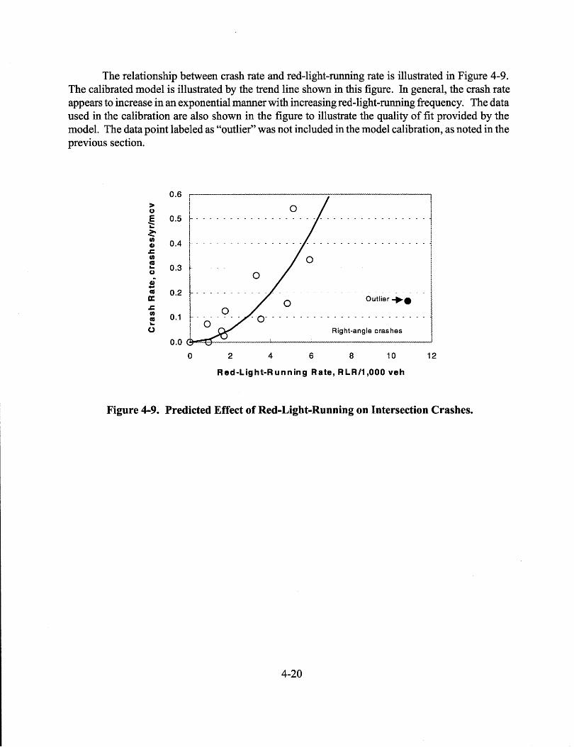
The relationship between crash rate and red-light-running rate is illustrated in Figure 4-9. The calibrated model is illustrated by the trend line shown in this figure. In general, the crash rate appears to increase in an exponential manner with increasing red-light-running frequency. The data used in the calibration are also shown in the figure to illustrate the quality of fit provided by the model. The data point labeled as "outlier" was not included in the model calibration, as noted in the previous section.

0.6 > ()

E 0.5 -... ~ U)

0.4 CD .c U) ca

0.3 ... ()

CD -ca 0.2 a: .c U) 0.1 ca ... 0

l • • • • • • • • • • • 0

• • • • • • • • • • • I l o I ~ - - - - - - - - - - - - - - - - - - - - - - - - - - - - - - - - - - i

I 0 !

l r ............ 0 ......... 6ut1;~,_. •. · 1 I 0 r- - - - - - - - - o- - - - - - - - - - - - - - - - - - - - - - - -! 0 I Right-angle crashes

0 2 4 6 8 10 12

Red-Light-Running Rate, RLR/1,000 veh

Figure 4-9. Predicted Effect of Red-Light-Running on Intersection Crashes.

4-20

CHAPTER 5. SUMMARY OF FINDINGS

OVERVIEW

Statistics indicate that red-light-running has become a significant safety problem throughout the United States. Mohamedshah et al. (2) estimate that at least 16 to 20 percent of intersection crashes can be attributed directly to red-light-running. Retting et al. ( 1) also report that motorists involved in red-light-running-related crashes are more likely to be injured than in other crashes. A 1998 survey of Texas drivers by the FHWA (3) found that two of three Texans witness red-light­running every day. About 89 percent of these drivers believe that red-light-running has worsened over the past few years.

There is a wide range of potential countermeasures to the red-light-running problem. These solutions are generally divided into two broad categories: engineering countermeasures and enforcement countermeasures. Enforcement countermeasures are intended to encourage drivers to adhere to the traffic laws through the threat of citation and possible fine. In contrast, engineering countermeasures are intended to reduce the chances of a driver being in a position where he or she must decide whether or not to run the red.

The objective of this research project is to describe how traffic engineering countermeasures can be used to minimize the frequency of red-light-running and associated crashes at urban intersections. This chapter documents the findings from the first year of research and the partial fulfillment of the research objective.

RED-LIGHT-RUNNING PROCESS

Influential Factors

A review of the literature revealed that red-light-running is the consequence of several events occurring together. They include the light changing to yellow while a vehicle is on the intersection approach, the vehicle's driver deciding not to stop, and the vehicle actually entering the intersection after the yellow interval has timed out. The following factors are related to the occurrence of these events and, thus, have some effect on the frequency ofred-light-running and related crash frequency:

• flow rate on the subject approach, • number of signal cycles, • phase termination by max-out, • probability of stopping, • yellow interval duration, • all-red interval duration, • entry time of the conflicting driver, and • flow rate on the conflicting approach.

5-1

Two fundamental factors that underlie the events leading to red-light-running include the probability-of-stopping and the yellow interval duration. The former factor represents the complex decision-making process that drivers exhibit at the onset of yellow. A review of the literature indicates that this decision is affected by the driver's assessment of the prevailing traffic and roadway conditions and by his or her estimate of the consequences of stopping (or not stopping). The yellow interval duration contributes in a more fundamental manner. The start of this interval defines the instant when the "signal" to stop is presented. The end of this interval defines the instant when the red indication is presented (whereupon entry to the intersection represents a red-light­running event).

Probability of Stopping

Many researchers have studied the decision to stop in response to the yellow indication. Van der Horst et al. (9) studied this decision process and found that a driver's propensity to stop is based on three components. These components include: (1) driver behavior (e.g., travel time, speed, approach grade, headway), (2) the consequences of not stopping (e.g., citation), and (3) the consequences of stopping (e.g., rear-end crash).

A review of the literature indicates that drivers are less likely to stop when they: ( 1) have a short travel time to the intersection, (2) have higher speeds, (3) are traveling in platoons, (4) are on steep downgrades, (5) are faced with relatively long yellow indications, and (6) are being closely followed. A driver is also likely to weigh the consequences of not stopping and of stopping when making his or her decision. Research indicates that drivers are less likely to stop if: ( 1) they believe the crossed street has a low traffic volume, (2) there is little threat of enforcement, (3) there is a threat ofrear-end collision, and (4) the expected delay is lengthy.

Yellow Interval Duration

The yellow interval duration is generally recognized as a key factor that affects the frequency of red-light-running. This recognition has led several researchers to recommend setting the yellow interval duration based on the probability of stopping (9, 12, 18). These researchers suggest that the yellow interval should be based on the travel time of the g5th (or 90th) percentile driver. The corresponding yellow interval duration should range from 4.0 to 5 .5 s (with larger values appropriate for higher-speed approaches). Data reported by Van der Horst and Wilmink (9) indicate that yellow intervals in excess of 3.5 s are associated with minimal red-light-running.

RED-LIGHT-RUNNING COUNTERMEASURES

Countermeasure Categories

There is a wide range of potential countermeasures to the red-light-running problem. These countermeasures are generally divided into two categories: engineering countermeasures and enforcement countermeasures. Enforcement countermeasures are intended to encourage drivers to

5-2

adhere to the traffic laws through the threat of citation and possible fine. In contrast, engineering countermeasures are intended to reduce the frequency that drivers are put in a position where they must decide whether or not to run the red.

There are two basic types of drivers who run red lights. The first is categorized as the "intentional" driver who runs the red light because of frustration or indifference resulting from excessive delay or congested flow conditions. Short of major resource investments to increase capacity, enforcement countermeasures are likely to be the most effective means of curbing this driver's inclination to run the red light. A nonscientific survey conducted by a news magazine of 4,711 readers revealed that 28 percent have intentionally run a red light (22).

The second driver type is the "unintentional" driver who runs the red light because he or she is incapable of stopping (e.g., due to a poorly judged downgrade or relatively high speed) or just inattentive (i.e., does not see the change to yellow). Engineering countermeasures, such as a longer yellow interval or a more visible signal indication, are likely to be the most effective means of helping these drivers avoid the need to run the red. The aforementioned news magazine survey found that most drivers ( 51 percent) are in the "unintentional" category.

Engineering Countermeasures

There is a wide range of potential engineering countermeasures to the red-light-running problem. Those countermeasures with the greatest potential to reduce red-light-running (as determined from the literature review) are listed in Table 5-1. The literature review and discussions with engineers in Texas indicated that the three countermeasures that are underlined in the table should be evaluated in this research project.

T bl 5 1 E a e - . n2meerm2 c t •th G t t P t f I oun ermeasures WI rea es o en Ia. Action Specific Countermeasure 1

Modify signal phasing, cycle length, or clearance Increase the yellow interval duration intervals

Provide green-extension

Im12rove signal coordination

Provide advance information or improved notification Improve sight distance

Im12rove visibilit'. of traffic control devices

Implement safety or operational improvements Remove unwarranted signals

Improve geometrics Note: 1 - Underlined countermeasures were selected for evaluation in this project.

5-3

FACTORS AFFECTING RED-LIGHT-RUNNING

This section describes the findings from an investigation of the factors that affect red-light­running. The findings presented are the result of a statistical analysis of a red-light-running database assembled for this research.

Model for Predicting the Frequency of Red-Light-Running

Analysis of approach volume on red-light-running frequency revealed that red-light-running frequency was highly correlated with the flow rate at the end of the phase. This flow rate is likely to be more intense in signalized street systems, particularly when the end of the platoon arrives to the approach at the end of the signal phase. In this situation, it is logical that more drivers are repetitively put in the position of having to decide to stop at the onset of yellow, relative to an isolated intersection or one where a larger majority of platoon drivers arrive at the start of green. Other factors found to be correlated with the frequency of red-light-running include yellow interval duration and the percentage of heavy vehicles.

A regression model was calibrated to predict the frequency of red-light-running. This model is offered as Equation 18 and is described in Chapter 4. The model includes variables for phase-end flow rate, cycle length, and "propensity," where the latter variable represents the propensity of drivers on a given intersection approach to "run the red light." It incorporates the effect of yellow interval duration and the percentage of heavy vehicles in the traffic stream. Guidance is also provided in Chapter 4 for estimating the phase-end flow rate based on a description of the quality of progression, as defined in Chapter 16 of the Highway Capacity Manual (33).

Sensitivity Analysis

A ·sensitivity analysis using the calibrated red-light-running model confirmed that yellow interval duration has a significant effect on red-light-running. Specifically, yellow intervals ofless than 3.5 s appear to be associated with a significant number of red-light-running events per hour. This finding is consistent with that noted previously when reviewing data reported by Van der Horst and Wilmink (9).

To a lesser extent, the presence of heavy vehicles also increases the number of vehicles running the red light. This increase is likely a result of the greater propensity of heavy-vehicle operators to run the red light.

EXAMINATION OF CRASH DATA

This section describes the findings from an investigation of the relationship between crash rate and the rate of red-light-running on an intersection approach. Least-squares, linear regression analysis was used to quantify the relationship between crash rate and red-light-running rate. The red­light-running rate was expressed as the number of red-light-runners per 1,000 approach vehicles.

5-4

A regression model was calibrated to predict the annual right-angle crash rate for an intersection approach. This model is offered as Equation 21 and is described in Chapter 4. The model includes a variable for the red-light-running rate on the subject approach. A sensitivity analysis using the calibrated crash rate model indicates that the right-angle crash rate increases in an exponential manner with increasing red-light-running frequency.

5-5

CHAPTER6. REFERENCES

1. Retting, R.A., A.F. Williams, and M.A. Greene. "Red-Light Running and Sensible Countermeasures." Transportation Research Record 1640. Transportation Research Board, Washington, D.C., 1998, pp. 23-26.

2. Mohamedshah, Y.M., L.W. Chen, and F.M. Council. "Association of Selected Intersection Factors with Red Light Running Crashes." Proceedings of the 701

h Annual ITE Conference. (CD-ROM). Institute of Transportation Engineers, Washington, D.C., August 2000.

3. Slemmons, B. "Two of Three Texans See Other Drivers Run Red Lights Almost Every Day." Press Release. Federal Highway Administration. Washington, D.C., September 4, 1998.

4. "Deaths in Red-Light-Running Crashes, By State, 1992-1998." News Release. Insurance Institute for Highway Safety, Arlington, Virginia, July 13, 2000.

5. Texas Transportation Code, Section 544. 007: Traffic-Control Signals in General. The Texas Statutes. Texas Legislative Council and West Group, July 2000. (http://www.capitol. state.tx.us/statutes/tr/tr054400.html#tr007 .544.007).

6. Parsonson, P.S., W.S. Czech, and W.C. Bansley, III. "Yellow and Red Clearance Signal Timing: Drivers and Attorneys Speak Out." ITE Journal, Institute of Transportation Engineers, Washington, D.C., June 1993, pp. 26-31.

7. Porter, B.E. and K.J. England. "Predicting Red-Light-Running Behavior: A Traffic Safety Study in Three Urban Settings." Journal of Safety Research, Vol. 31, No. 1, Elsevier Science Ltd, Spring 2000, pp. 1-8.

8. Baguley, C.J. "Running the Red at Signals on High-Speed Roads." Traffic Engineering & Control. Crowthome, England, July/August 1988, pp. 415-420.

9. Van der Horst, R. and A.Wilmink. "Drivers' Decision-Making at Signalized Intersections: An Optimization of the Yellow Timing." Traffic Engineering & Control. Crowthome, England, December 1986, pp. 615-622.

10. Zegeer, C.V. and R.C. Deen. "Green-Extension Systems at High-Speed Intersections." ITE Journal, Institute of Transportation Engineers, Washington, D.C., November 1978, pp. 19-24.

11. Bonneson, J .A. and P. T. McCoy. "Traffic Detector Designs for Isolated Intersections." ITE Journal, Institute of Transportation Engineers, Washington, D.C., August 1996, pp. 42-47.

6-1

12. Olson, P.L. and R.W. Rothery. "Driver Response to the Amber Phase of Traffic Signals." Traffic Engineering. Institute of Traffic Engineers, Washington, D.C., February 1962, pp. 17-29.

13. Williams, W.L. "Driver Behavior During the Yellow Interval." Transportation Research Record 644. Transportation Research Board, Washington, D.C., 1977, pp. 75-78.

14. Hulsher, F.R. "The Problem of Stopping Drivers after the Termination of the Green Signal at Traffic Lights." Traffic Engineering and Control." Crowthome, England, March 1984, pp. 110-116.

15. Sheffi, Y. and H. Mahmassani. "A Model of Driver Behavior at High Speed Signalized Intersections." Transportation Science. Vol. 15, No. 1, February 1981, pp. 50-61.

16. Bonneson, J.A., P.T. McCoy, and B.A. Moen. Traffic Detector Design and Evaluation Guidelines. Report No. TRP-02-31-93. Nebraska Dept. of Roads, Lincoln, Nebraska, April 1994.

17. Allsop, R.E., I.D. Brown, J.A. Groeger, and S.A. Robertson. Contractor Report 264: Approaches to Modelling Driver Behavior at Actual and Simulated Traffic Signals. Transport and Road Research Laboratory, Crowthome, England, 1991.

18. Chang, M., C.J. Messer, and A.J. Santiago. "Timing Traffic Signal Change Intervals Based on Driver Behavior." Transportation Research Record 1027. Transportation Research Board, Washington, D.C., 1985, pp. 20-30.

19. Mahalel, D. and J.N. Prashker. "A Behavioral Approach to Risk Estimation of Rear-End Collisions at Signalized Intersections." Transportation Research Record 1114. Transportation Research Board, Washington D.C., 1987, pp. 96-102.

20. Retting, R.A. and A.F. Williams. "Red Light Cameras and the Perceived Risk of Being Ticketed." Traffic Engineering and Control. Vol. 41, No. 6. Crowthome, England, June 2000, pp. 224-229.

21. Manual on Uniform Traffic Control Devices. U.S. Department of Transportation, Federal Highway Administration, U.S. Government Printing Office, Washington, D.C., 1988.

22. "Quick Results Question." Web survey. USA TODAY, Gannett Co, Inc., July 13, 2000.

23. Retting, R.A. and M.A. Greene. "Influence of Traffic Signal Timing on Red-Light Running and Potential Vehicle Conflicts at Urban Intersections." Transportation Research Record 15 9 5. Transportation Research Board, Washington D.C., 1997, pp. 1-7.

6-2

24. Hagenauer, G.F., J. Upchurch, D. Warren, and M.J. Rosenbaum. "Chapter 5 -Intersections." Synthesis of Safety Research Related to Traffic Control and Roadway Elements. Vol. 1. Report No. FHW A-TS-82-232. Federal Highway Administration, Washington, D.C., December 1982.

25. Farraher, B.A., R.Weinholzer, and M.P. Kowski. "The Effect of Advanced Warning Flashers on RedLight Running -A Study Using Motion Imaging Recording System Technology at Trunk Highway 169 and Pioneer Trail in Bloomington, Minnesota." Compendium of Technical Papers for the 69th Annual !TE Meeting. (CD:.ROM) Institute of Transportation Engineers, Washington, D.C., 1999.

26. McCullagh, P. and J.A. Nelder. Generalized Linear Models, Chapman and Hall, New York, New York, 1983.

27. Hauer, E., J.C. Ng, and J.J. Lovell. "Estimation of Safety at Signalized Intersections." In Transportation Research Record 1185, TRB, National Research Council, Washington, D.C., 1988, pp. 48-61.

28. Bonneson, J.A. and P.T. McCoy. "Effect of Median Treatment on Urban Arterial Safety: An Accident Prediction Model." Transportation Research Record 1581, Transportation Research Board, Washington, D.C., 1997, pp. 27-36.

29. SAS/STAT User's Guide, Version 6, 4th ed., SAS Institute, Inc., Cary, North Carolina, 1990.

30. Abbess, C., D. Jarrett, and C.C. Wright. "Accidents at Black-Spots: Estimating the Effectiveness of Remedial Treatment, with Special Reference to the 'Regression-to-the-Mean' Effect." Traffic Engineering and Control, Vol. 22, No. 10, October 1981, pp. 535-542.

31. Kvalseth, T.O. "Cautionary Note About R2." The American Statistician, Vol. 39, No. 4,

(Part 1), American Statistical Association, November 1985, pp. 279-285.

32. Determining Vehicle Signal Change and Clearance Intervals. Prepared by Technical Council Task Force 4TF-1. Institute of Transportation Engineers, Washington, D.C., August 1994.

33. Highway Capacity Manual 2000. 4th ed. Transportation Research Board, Washington, D.C., 2000.

6-3

APPENDIX

TEXAS TRANSPORTATION CODE

CHAPTER544

A-1

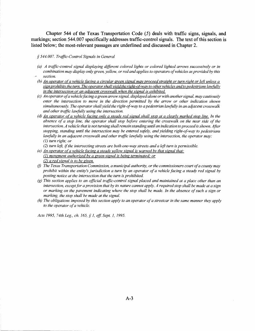
Chapter 544 of the Texas Transportation Code (5) deals with traffic signs, signals, and markings; section 544.007 specifically addresses traffic-control signals. The text of this section is listed below; the most-relevant passages are underlined and discussed in Chapter 2.

§ 544.007. Traffic-Control Signals in General

(a) A traffic-control signal displaying different colored lights or colored lighted arrows successively or in combination may display only green, yellow, or red and applies to operators of vehicles as provided by this section.

(b) An operator ofa vehicle facing a circular green signal may proceed straight or turn right or left unless a sign prohibits the turn. The operator shall yield the right-of-way to other vehicles and to pedestrians lawfully in the intersection or an adjacent crosswalk when the signal is exhibited.

(c) An operator of a vehicle facing a green arrow signal, displayed alone or with another signal, may cautiously enter the intersection to move in the direction permitted by the arrow or other indication shown simultaneously. The operator shall yield the right-of-way to a pedestrian lawfully in an adjacent crosswalk and other traffic lawfully using the intersection. ,

(d) An operator ofa vehicle facing only a steady red signal_shall stop at a clearly marked stop line. In the absence of a stop line, the operator shall stop before entering the crosswalk on the near side of the intersection. A vehicle that is not turning shall remain standing until an indication to proceed is shown. After stopping, standing until the intersection may be entered safely, and yielding right-of-way to pedestrians lawfully in an adjacent cro~swalk and other traffic lawfully using the intersection, the operator may: (1) turn right; or (2) turn left, if the intersecting streets are both one-way streets and a left turn is permissible.

(e) An operator ofa vehicle facing a steady ye/low signal is warned by that signal that: (]) movement authorized by a green signal is being terminated; or (2) a red signal is to be given.

(j) The Texas Transportation Commission, a municipal authority, or the commissioners court of a county may prohibit within the entity's jurisdiction a turn by an operator of a vehicle facing a steady red signal by posting notice at the intersection that the turn is prohibited.

(g) This section applies to an official traffic-control signal placed and maintained at a place other than an intersection, except for a provision that by its nature cannot apply. A required stop shall be made at a sign or marking on the pavement indicating where the stop shall be made. In the absence of such a sign or marking, the stop shall be made at the signal.

(h) The obligations imposed by this section apply to an operator of a streetcar in the same manner they apply to the operator of a vehicle.

Acts 1995, 74th Leg., ch. 165, § 1, ejf. Sept. 1, 1995.

A-3