ISSN 0280–5316ISRN LUTFD2/TFRT­­7607­­SE

Review of Wheel Modelingand Friction Estimation

Jacob SvendeniusBjörn Wittenmark

Department of Automatic ControlLund Institute of Technology

Augusti 2003

Department of Automatic Control

Lund Institute of TechnologyBox 118

SE­221 00 Lund Sweden

Document name

INTERNAL REPORTDate of issue

August 2003Document Number

ISRN LUTFD2/TFRT­­7607­­SE

Author(s)

Jacob SvendeniusSupervisor

Björn Wittenmark

Sponsoring organisationHaldex Brake Products AB

Title and subtitleReview of Wheel Modeling and Friction Estimation

Abstract

In this report research about tire modeling and friction estimation is collected and resumed. The reportalso covers the brush­model explanation to the slip phenomenon that comes up when the rim transmitsa force to the ground through the tire when the wheel is rolling. The term slip significance the differencebetween the wheel velocity and the vehicle velocity when a driving or braking force is working on thetire. Most of the approaches that estimate tire friction build on the relation between the slip and theforce that works on the tire. The paper also describes a couple of ways to include an extra calibrationparameter in the brush model to improve its accuracy and enhance the friction estimation at low forceexcitations. Finally, results from simulation of friction estimation are presented.

Key words

Tire Model, Brush Model, Slip, Friction Estimation

Classification system and/or index terms (if any)

Supplementary bibliographical information

ISSN and key title0280–5316

ISBN

LanguageEnglish

Number of pages38

Security classification

Recipient’s notes

The report may be ordered from the Department of Automatic Control or borrowed through:University Library 2, Box 3, SE­221 00 Lund, SwedenFax +46 46 222 44 22 E­mail ub2@ub2.lu.se

Contents

1. Introduction . . . . . . . . . . . . . . . . . . . . . . . . . . . 52. Tire modeling . . . . . . . . . . . . . . . . . . . . . . . . . . 5

2.1 Vertical deformation pressure distribution . . . . . . . 52.2 Inputs and output for horizontal tire modeling . . . . 72.3 Brush model . . . . . . . . . . . . . . . . . . . . . . . . . 92.4 Empirical models . . . . . . . . . . . . . . . . . . . . . . 14

3. Estimation models . . . . . . . . . . . . . . . . . . . . . . . 163.1 Slip based friction estimation according to NIRA­dynamics 163.2 Brake force estimation with a Kalman­Busy Filter . . 173.3 GPS­based identification of the lateral tire­road fric­

tion coefficient . . . . . . . . . . . . . . . . . . . . . . . 183.4 Optimal braking and friction estimation with the Lu­

Gre model . . . . . . . . . . . . . . . . . . . . . . . . . . 193.5 Extended Braking Stiffness (XBS) . . . . . . . . . . . . 193.6 Lateral friction estimation using the brush tire model 203.7 Longitudinal friction estimation using the brush tire

model . . . . . . . . . . . . . . . . . . . . . . . . . . . . . 203.8 Friction estimation for vehicle path prediction . . . . 213.9 Discussion . . . . . . . . . . . . . . . . . . . . . . . . . . 22

4. Changes to the Brush Tire Model to Enhance Fric­

tion Estimation . . . . . . . . . . . . . . . . . . . . . . . . . 224.1 Pressure distribution . . . . . . . . . . . . . . . . . . . . 234.2 Velocity dependent friction . . . . . . . . . . . . . . . . 274.3 Taylor expansion . . . . . . . . . . . . . . . . . . . . . . 304.4 Velocity dependency . . . . . . . . . . . . . . . . . . . . 31

5. Simulation of Friction Estimation with Brush Model 325.1 Data generation . . . . . . . . . . . . . . . . . . . . . . 325.2 Estimation of brush model parameters . . . . . . . . . 325.3 Estimation results . . . . . . . . . . . . . . . . . . . . . 345.4 Effect of the calibrating d­factor . . . . . . . . . . . . . 35

6. Conclusions . . . . . . . . . . . . . . . . . . . . . . . . . . . 367. References . . . . . . . . . . . . . . . . . . . . . . . . . . . . 38

3

4

1. Introduction

In this report research about tire modeling and friction estimation is col­lected and resumed. It also covers the brush­model explanation to the slipphenomenon that comes up when the rim transmits a force to the groundthrough the tire when the wheel is rolling. The term slip significance thedifference between the wheel velocity and the vehicle velocity when a driv­ing or braking force is working on the tire. Most of the approaches thatestimate tire friction build on the relation between the slip and the forcethat works on the tire. The paper also describes a couple of ways to includean extra calibration parameter in the brush model to improve its accuracyand enhance the friction estimation at low excitations. Finally, results fromsimulation of friction estimation are presented.

The brush­model used for the estimation and empirical tire model aredescribed in Section 2 The estimation review, Section 3, presents tech­niques developed by among others F. Gustafsson [6], L. Ray [16] and C.Canudas de Wit [4]. Section 4 contains an extension of the brush modeland simulated estimation results are given in Section 5.

2. Tire modeling

The main purpose of a tire is to transmitt forces between the road and therim so that the driver can control the vehicle. The tire also works as a lowpass filter in the suspension system by reducing the high frequency vibra­tions from small unevenesses in the road. A lot of work has been done inthe area of modeling tires and it covers everything from simple models aim­ing for understanding the physics to advanced finite­element models thatcan predict the behavior precisely. An exact analysis of the tire and itsdynamical properties is very complex and is not realistic to implement in avehicle system. Since the properties of different tires differ a lot the systemhas to know these properties when the tire is changed. The properties alsochange by wear, temperature, road conditions, etc. Therefore, researchershave developed empirical models including a few parameters, which canbe determined by testing the tire. These models can then be used for calcu­lations in simulations or real­time implementations. The possibility to usethese models in a vehicle system is better, but still limited since factorsfrom the driving environment affect the friction properties. The modelingin this paper will be very basic, with the aim to make the reader under­stand the physics behind the slip behavior of tires. The model is aimed tobe general and the number of parameters is kept as low as possible.

2.1 Vertical deformation pressure distribution

Exposed to a vertical load the tire will deform. An exact analysis of the de­formation requires good calculation tools and accurate information aboutthe tire design and actual conditions, as axle load, road surface, and tem­perature. Schematicly, the deformation can be divided into two parts. Onepart from the change of the carcass shape and one from the compression ofthe rubber material. If the carcass deformation is moderate the air volumein the tire will remain nearly constant and no consideration to increasedtire pressure is necessary. In the static case, i.e. when the wheel is not

5

0 a

p0 Carc

ass

Rubber

Road

qz(x)

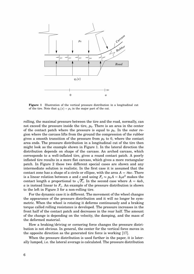
Figure 1 Illustration of the vertical pressure distribution in a longitudinal cutof the tire. Note that qz(x) = p0 in the major part of the cut.

rolling, the maximal pressure between the tire and the road, normally, cannot exceed the pressure inside the tire, p0. There is an area in the centerof the contact patch where the pressure is equal to p0. In the outer re­gion where the carcass lifts from the ground the compression of the rubbergives a smooth transition of the pressure from p0 to 0, where the contactarea ends. The pressure distribution in a longitudinal cut of the tire thenmight look as the example shown in Figure 1. In the lateral direction thedistribution depends on shape of the carcass. An arched carcass, whichcorresponds to a well­inflated tire, gives a round contact patch. A poorlyinflated tire results in a more flat carcass, which gives a more rectangularpatch. In Figure 2 these two different special cases are shown and anyintermediate solution is realistic. In the first case it is assumed that thecontact zone has a shape of a circle or ellipse, with the area A = π ac. Thereis a linear relation between a and c and using Fz p0 A = k0a2 makes thecontact length a proportional to

√Fz. In the second case where A = 4ab,

a is instead linear to Fz. An example of the pressure distribution is shownto the left in Figure 3 for a non­rolling tire.

For the dynamic case it is different. The movement of the wheel changesthe appearance of the pressure distribution and it will no longer be sym­metric. When the wheel is rotating it deforms continuously and a brakingtorque called rolling resistance is developed. The pressure increases in thefront half of the contact patch and decreases in the rear half. The amountof the change is depending on the velocity, the damping, and the mass ofthe deformed material.

How a braking/driving or cornering force changes the pressure distri­bution is not obvious. In general, the center for the vertical force moves inthe opposite direction as the generated tire force is working [17].

When the pressure distribution is used further in the paper, it is later­ally lumped, i.e. the lateral average is calculated. The pressure distribution

6

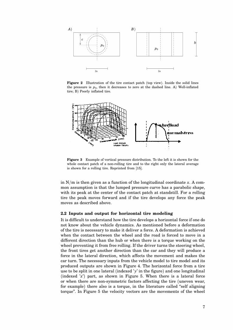
2a2a

cb

A) B)

p0p0

Figure 2 Illustration of the tire contact patch (top view). Inside the solid linesthe pressure is p0, then it decreases to zero at the dashed line. A) Well­inflatedtire; B) Poorly inflated tire.

Figure 3 Example of vertical pressure distribution. To the left it is shown for thewhole contact patch of a non­rolling tire and to the right only the lateral averageis shown for a rolling tire. Reprinted from [15].

in N/m is then given as a function of the longitudinal coordinate x. A com­mon assumption is that the lumped pressure curve has a parabolic shape,with its peak at the center of the contact patch at standstill. For a rollingtire the peak moves forward and if the tire develops any force the peakmoves as described above.

2.2 Inputs and output for horizontal tire modeling

It is difficult to understand how the tire develops a horizontal force if one donot know about the vehicle dynamics. As mentioned before a deformationof the tire is necessary to make it deliver a force. A deformation is achievedwhen the contact between the wheel and the road is forced to move in adifferent direction than the hub or when there is a torque working on thewheel preventing it from free rolling. If the driver turns the steering wheel,the front tires get another direction than the car and they will produce aforce in the lateral direction, which affects the movement and makes thecar turn. The necessary inputs from the vehicle model to tire model and itsproduced outputs are shown in Figure 4. The horizontal force from a tireuse to be split in one lateral (indexed ’y’ in the figure) and one longitudinal(indexed ’x’) part, as shown in Figure 5. When there is a lateral forceor when there are non­symmetric factors affecting the tire (uneven wear,for example) there also is a torque, in the literature called “self aligningtorque”. In Figure 5 the velocity vectors are the movements of the wheel

7

hub and the forces are working in the contact patch between tire and theroad.

y

xF

F

Longitudinal force

Lateral force

xM Self aligning torque

Output

Ω Angular velocity

F z Vertical load

x Longitudinal speed

y Lateral speed

Movement of wheelhub

Whe

elV

ehic

le

Input

v

v

Figure 4 Basic input­output signals for a tire model.

vx

vy

vs v

Fx

Fy

Mz

ΩRe

Figure 5 Forces and movements in a tire model. Re is the rolling radius of thetire.

Slip Definitions One of the mostly used terms in tire modeling is slip. Itcan be defined in a couple of ways and the difference between the definitionsis how to normalize the slip velocity.

Origin Notation Long. Lateral

SAE, ISO κ vsx/vx vy/vx

Praxis s vsx/hvh vy/hvhPhysical σ vsx/(ΩRe) vy/(ΩRe)

Table 1 Slip definitions. Note that vsx = vx −ΩRe , i.e. the longitudinal componentof vs.

The definition denoted s is the most convenient definition. It gets singu­lar only at standstill of the vehicle and the value will always stay between−1 and 1, when braking or cornering (for driving often σ is used since it

8

always has proper values then). The other definitions (κ , σ ) get singular ei­ther at wheel­lock or when the car only has lateral velocity. In Section 2.3an expression depending on σ x is derived. The slip denoted by σ corre­sponds to the deformation of the rubber in the tire contact patch. s and κcorresponds to the relative velocity between the tire and the road. For theempirical modeling the main thing may not be how to define the slip, butrather to know which definition that has been used for the measurements.

2.3 Brush model

In the brush model [13] it is assumed that the slip is caused by deformationof the rubber volume that is between the tire carcass and the ground. Thevolume is approximated as small brush elements, attached to the carcass,see Figure 6. The carcass is assumed to be stiff and it can neither stretchnor shrink, but it can still flex towards the hub. Every brush element candeform independently of the other.

A brush element i comes in contact with the road at time t=0 and atthe position x = a.The position of an element can be defined at its upperpoint (xic, attached to the carcass) or at its lower point (xir, the contact tothe road), see Figure 7. As long as there is no sliding the positions will be

xci = a −∫ t

0ΩRe dt (1)

xri = a −∫ t

0vx dt (2)

The deformation of the element is:

δ i = xci − xri =∫ t

0vx − ΩRe dt =

∫ t

0vsx dt (3)

If constant velocities are assumed, (3) together with (1) or (2) gives

δ i = vsx

ΩRe(a − xci) = vsx

vx(a − xri) (4)

where vsx/(ΩRe) is the longitudinal slip denoted σ x.

Road

CarcassRubber

AdhesionSlide

vsx

a−a xs

x0

Figure 6 Illustration showing the deformation of the rubber layer between thetire carcass and the road according to the brush model. The carcass moves withthe velocity vsx relative the road. The contact zone moves with the vehicle velocityvx.

9

−δ

Road

Carcass

Road

Rubber

Carcass

Rubber

Fxi

Fxi

Fzi

Fzi

Myi

ΩRe

vx

xci

xri

xx

zz

A) B)

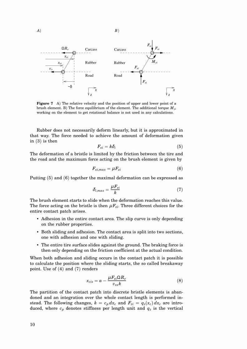
Figure 7 A) The relative velocity and the position of upper and lower point of abrush element. B) The force equilibrium of the element. The additional torque Myi

working on the element to get rotational balance is not used in any calculations.

Rubber does not necessarily deform linearly, but it is approximated inthat way. The force needed to achieve the amount of deformation givenin (3) is then

Fxi = kδ i (5)The deformation of a bristle is limited by the friction between the tire andthe road and the maximum force acting on the brush element is given by

Fxi,max = µ Fzi (6)

Putting (5) and (6) together the maximal deformation can be expressed as

δ i,max = µ Fzi

k(7)

The brush element starts to slide when the deformation reaches this value.The force acting on the bristle is then µ Fzi. Three different choices for theentire contact patch arises.

• Adhesion in the entire contact area. The slip curve is only dependingon the rubber properties.

• Both sliding and adhesion. The contact area is split into two sections,one with adhesion and one with sliding.

• The entire tire surface slides against the ground. The braking force isthen only depending on the friction coefficient at the actual condition.

When both adhesion and sliding occurs in the contact patch it is possibleto calculate the position where the sliding starts, the so called breakawaypoint. Use of (4) and (7) renders

xcis = a − µ FziΩRe

vsxk(8)

The partition of the contact patch into discrete bristle elements is aban­doned and an integration over the whole contact length is performed in­stead. The following changes, k = cp dxc and Fzi = qz(xc) dxc are intro­duced, where cp denotes stiffness per length unit and qz is the vertical

10

force per length unit between tire and road. Adding the force from thearea of adhesion to the force from the sliding region the total braking forceis

Fx =∫ a

xcs

cpvsx

ΩRe

(a − xc) dxc +∫ xcs

a

qz(xc)µ dxc (9)

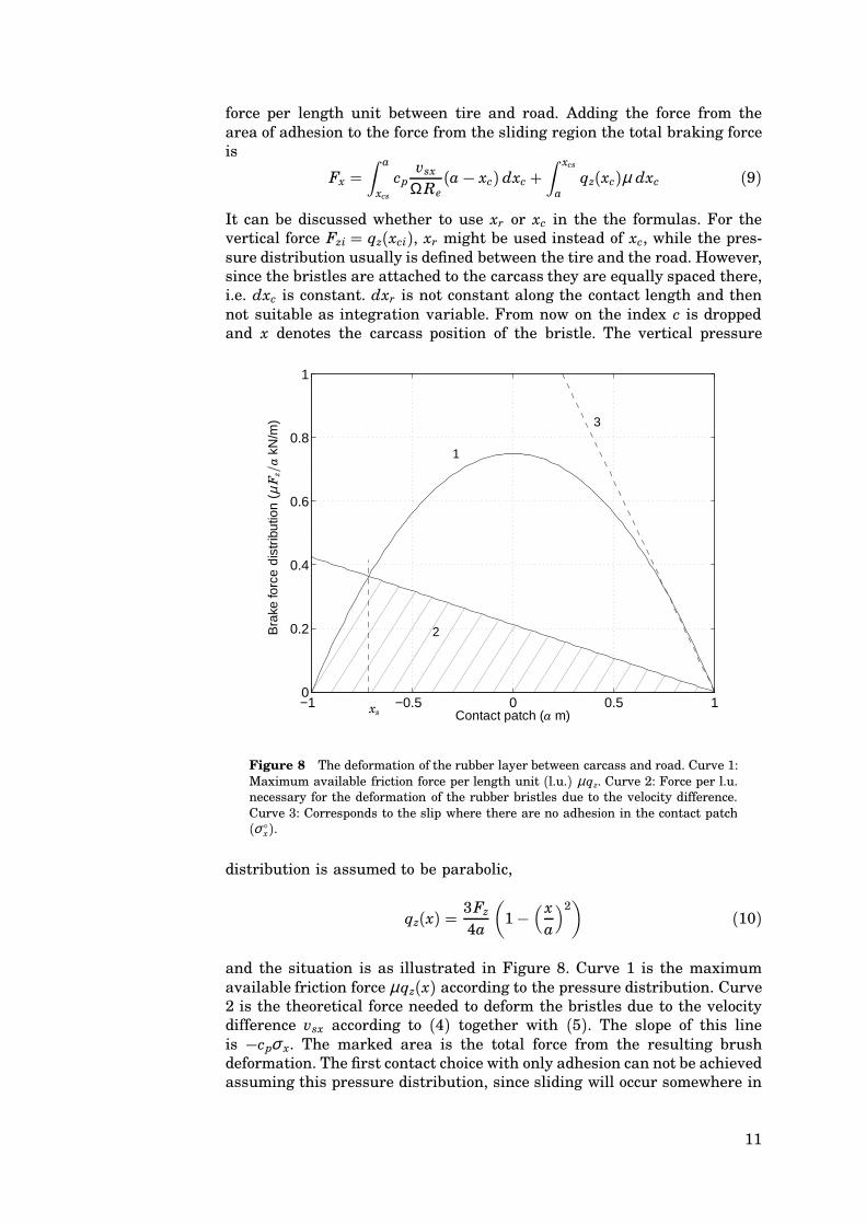
It can be discussed whether to use xr or xc in the the formulas. For thevertical force Fzi = qz(xci), xr might be used instead of xc, while the pres­sure distribution usually is defined between the tire and the road. However,since the bristles are attached to the carcass they are equally spaced there,i.e. dxc is constant. dxr is not constant along the contact length and thennot suitable as integration variable. From now on the index c is droppedand x denotes the carcass position of the bristle. The vertical pressure

−1 −0.5 0 0.5 10

0.2

0.4

0.6

0.8

1

2

1

3

xs Contact patch (a m)

Bra

kefo

rce

dist

ribut

ion

(µF

z/a

kN/m

)

Figure 8 The deformation of the rubber layer between carcass and road. Curve 1:Maximum available friction force per length unit (l.u.) µqz. Curve 2: Force per l.u.necessary for the deformation of the rubber bristles due to the velocity difference.Curve 3: Corresponds to the slip where there are no adhesion in the contact patch(σ

x).

distribution is assumed to be parabolic,

qz(x) = 3Fz

4a

(

1 −( x

a

)2)

(10)

and the situation is as illustrated in Figure 8. Curve 1 is the maximumavailable friction force µqz(x) according to the pressure distribution. Curve2 is the theoretical force needed to deform the bristles due to the velocitydifference vsx according to (4) together with (5). The slope of this lineis −cpσ x. The marked area is the total force from the resulting brushdeformation. The first contact choice with only adhesion can not be achievedassuming this pressure distribution, since sliding will occur somewhere in

11

0 0.1 0.2 0.3 0.4 0.50

0.2

0.4

0.6

0.8

Slip

Nor

mal

ized

bra

ke fo

rce

0 0.1 0.2 0.3 0.4 0.50

0.2

0.4

0.6

0.8

Slip

Nor

mal

ized

bra

ke fo

rce

Figure 9 Normalized brake force contra longitudinal slip (σ x) with different val­ues of µ and cp. Parabolic (left) and uniform (right) pressure distribution is usedin the calculations.

the region as long as the slip is nonzero. The breakaway point xs can bederived from the following formula

cpσ (a − xs) = µqz(xs) (11)

Evaluating (9) with the pressure distribution given by (10) the equationfor the force­slip will be

Fx = 2cpa2σ x − 43

(cpa2σ x)2

µ Fz+ 8

27(cpa2σ x)3

(µ Fz)2 (12)

According to this expression the slip behavior is mainly dependent on thetire properties at low slip. Often the relation between the force and theslip in this region is assumed to be linear with a coefficient called brakingstiffness Cx. In this case Cx = 2cpa2. At higher slip the friction coefficientis the major source for the characteristics. If the inclination of Curve 2 inFigure 8 is steeper than the inclination of Curve 1 at x = a the entiresurface will slide, which is illustrated by Curve 3. Hence, the incline of thepressure distribution at x = a sets the slip limit where the entire rubbersurface starts to slide against the road. In this case it is given by

σ xt = 32

µ Fz

cpa2 (13)

If the slip exceeds this value the braking force will simply be put to Fx =µ Fz.

Fx(σ x) is shown in Figure 9. Since constant friction is assumed thebrake force is constant for slip values above σ xt.

Uniform pressure distribution To show the importance of the verticalpressure distribution the calculation from above has been done assuminguniform pressure. Let qz denote the force per length unit.

qz(x) = Fz

2a

The point where sliding starts can be derived by reformulation of equation(8), hence

xs = a − µ Fz

2cpaσ

12

For xs < −a there is no sliding and the expression for the brake force isderived from the first integral in (9) using xcs = a. In the other case thewhole expression (9) is used That gives

Fx =

2cpa2σ if σ < µ Fz/(4cpa2)

Fzµ − F2z µ2

4a2cpσ xotherwise

(14)

The result is shown in Figure 9. For uniform pressure we never reallyget the entire contact patch to slide, which can be seen on the asymptoticconvergence to µ when the slip increases.

Lateral slip In the lateral direction the effects of the flexibility of thecarcass normally, is larger than in the longitudinal direction [13]. For betteraccuracy its deformation should be included in the model. The literaturemainly describes two ways to handle this. The simpler one is the threadmodel where the carcass is treated as a thread. The more complicated isthe beam model where the deformation is calculated according to the beamtheory.

Deformation of the carcass according to the thread model is given by

Sd2δ c(x)

dx2 = pc y(x) (15)

S is the tension in the thread. p is the horizontal force per length unit.Index ’c’ denotes carcass and ’b’ brush. Deformation of the rubber as in thelongitudinal case

pby(x) = cpyδ b(x)Total deformation of the brush in contact with the road is

δ y = vsy

vxx

The carcass and the brush element can be treated as connected seriallywhich means that the total deformation is the sum of the two elements.The force acting on the brush is the same as the force acting on the corre­sponding point of carcass. This gives

δ y = δ c + δ b

pby = pc y = py

From this we get the following differential equation for the lateral forceper length unit

d2

dx

(

vsy

vxx − py(x)

cpy

)

= py(x)

Which has to be solved with the constraint that py(x) can not exceed µqz.After having solved this equation with suitable initial conditions the totallateral force is derived by

Fy =∫ a

−a

pry dx

13

If the beam model is used instead of the thread model the second derivativeif equation (15) has to be exchanged for a derivative of the fourth order.The equation is rather complicated and will not be solved in this paper. Asimpler approach is to assume a certain shape of the carcass deformationwith an amplitude depending on the total lateral force.

Combined slip When there is both longitudinal and lateral slip correc­tions are necessary. In the case that the tire has isotropic properties (i.e.equal in all directions) the resultant of the slip vector (σ 2

x + σ 2y)1/2 can be

used in the force­slip formula and the tire force acts in the opposite direc­tion as the slip vector. A tire is, in general, not isotropic as discussed aboveand in [13] and [5] it is explained how the brush model can be expandedinto two dimensions assuming anisotropic conditions. For empirical mod­els, see Section 2.4, there are a lot of suggested solutions how to derive theforce­slip relation for any direction of the slip vector given the results frompure lateral and pure longitudinal slip. One solution is explained in [5],which has the following important features:

• It reduces exactly to the empirical model at pure­slip.

• It gives a smooth transition from small­slip to large­slip behavior thatagrees with empirical observations.

• Only few parameters are needed, which all have clear physical inter­pretations.

• Nominal parameter values may be derived automatically from theempirical pure­slip models.

• Differences between driving and braking conditions are accounted for.

Discussion This section has mainly treated the way to physically derivea relation between the braking force and the slip. The resulting expressionincludes the rubber stiffness cp, the length of the contact patch 2 a, thetire/road friction µ , and the vertical wheel load Fz. The vertical pressuredistribution qz(x) is another very important factor for the formula. cp isa material parameter and is depending on the rubber thickness, i.e. itwill increase when the tire wears. It is probably also depending on thetemperature in the tire. In Section 2.1 there is a discussion about therelation between a and Fz. The friction is the most uncertain parameterand it is affected by factors such as road condition, slip velocity, and treadthickness. How different relations between the friction coefficient and therelative velocity affects the force­slip curve is treated in Section 4.2.

2.4 Empirical models

Two famous empirical models to describe the input­output formulas for atire are presented in this section.

Magic Formula In [2] H. B. Pacejka presents the Magic Formula whichis very well suited for describing the force­slip function as

F = D sin (C arctan (Bλ − E(Bλ − arctan Bλ))) (16)

The parameters B, C, D, and E have to be identified through measure­ment data. Both the longitudinal and lateral force can be expressed in this

14

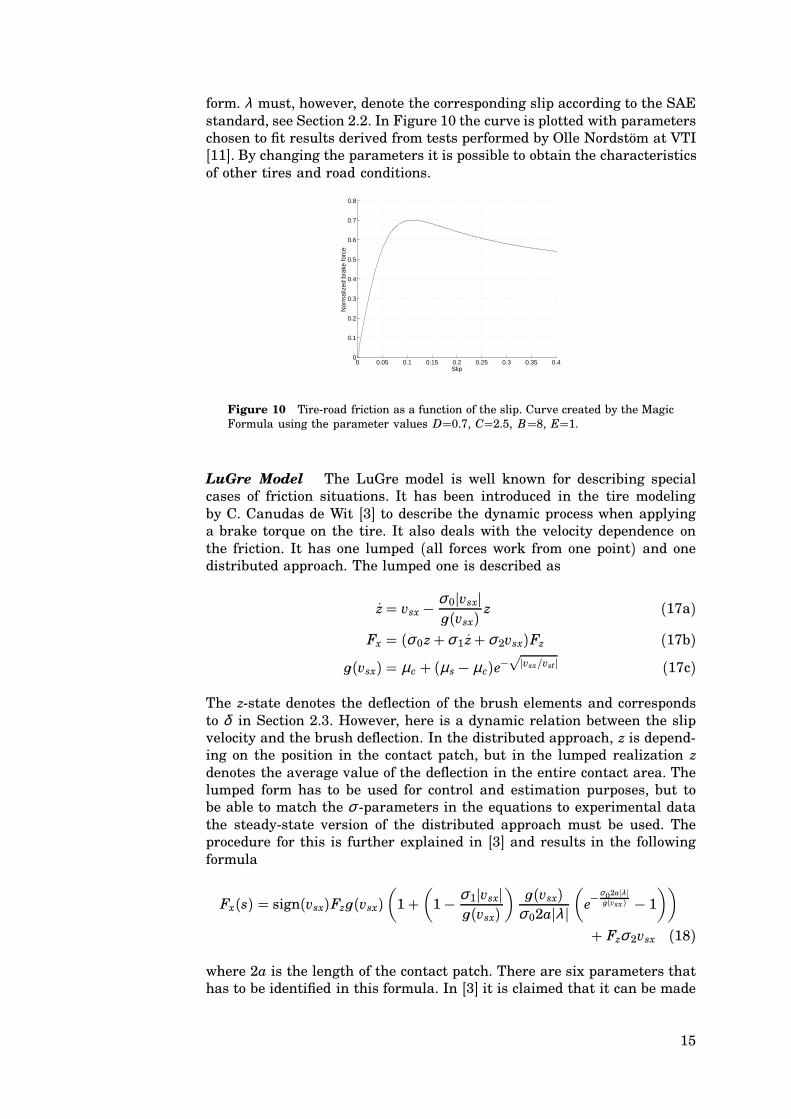
form. λ must, however, denote the corresponding slip according to the SAEstandard, see Section 2.2. In Figure 10 the curve is plotted with parameterschosen to fit results derived from tests performed by Olle Nordstöm at VTI[11]. By changing the parameters it is possible to obtain the characteristicsof other tires and road conditions.

0 0.05 0.1 0.15 0.2 0.25 0.3 0.35 0.40

0.1

0.2

0.3

0.4

0.5

0.6

0.7

0.8

Slip

Nor

mal

ized

bra

ke fo

rce

Figure 10 Tire­road friction as a function of the slip. Curve created by the MagicFormula using the parameter values D=0.7, C=2.5, B=8, E=1.

LuGre Model The LuGre model is well known for describing specialcases of friction situations. It has been introduced in the tire modelingby C. Canudas de Wit [3] to describe the dynamic process when applyinga brake torque on the tire. It also deals with the velocity dependence onthe friction. It has one lumped (all forces work from one point) and onedistributed approach. The lumped one is described as

z = vsx − σ 0hvsxhn(vsx)

z (17a)

Fx = (σ 0z + σ 1 z + σ 2vsx)Fz (17b)

n(vsx) = µc + (µs − µc)e−√

hvsx/vsth (17c)

The z­state denotes the deflection of the brush elements and correspondsto δ in Section 2.3. However, here is a dynamic relation between the slipvelocity and the brush deflection. In the distributed approach, z is depend­ing on the position in the contact patch, but in the lumped realization z

denotes the average value of the deflection in the entire contact area. Thelumped form has to be used for control and estimation purposes, but tobe able to match the σ ­parameters in the equations to experimental datathe steady­state version of the distributed approach must be used. Theprocedure for this is further explained in [3] and results in the followingformula

Fx(s) = sign(vsx)Fzn(vsx)(

1 +(

1 − σ 1hvsxhn(vsx)

) n(vsx)σ 02ahλ h

(

e− σ02ahλ h

n(vsx) − 1))

+ Fzσ 2vsx (18)

where 2a is the length of the contact patch. There are six parameters thathas to be identified in this formula. In [3] it is claimed that it can be made

15

look very similar to the shape of Magic Formula. In Figure 11 there isan example a force­slip curve generated by the LuGre model. This curveshould not be compared to the curve in Figure 10, since the parameters forthe LuGre model are not identified from that curve.

0 0.1 0.2 0.3 0.4 0.5 0.6 0.7 0.8 0.9 10

0.1

0.2

0.3

0.4

0.5

0.6

0.7

0.8

Slip

Nor

mal

ized

bra

ke fo

rce

Figure 11 Static force­slip curve generated with the LuGre­model, trying tomatch the Magic Formula shape

Discussion Two empirical models for describing the force­slip relationhave been described above. Many more models are described in the liter­ature, but after the introduction of the Magic Formula, it has become theabsolutely most popular tire model. The LuGre­model is interesting whileit tries to deal with the dynamics in the friction surface.

3. Estimation models

3.1 Slip based friction estimation according to NIRA­dynamics

Estimation of the road­tire friction by examining the slip­force curve hasbeen done by F. Gustavsson [6]. The assumption is that for low slip valuesthe relation between the force and the slip is

F = ks

It is then stated that k is not only tire depending it is also depending onthe tire­road friction µ . By using a Kalman filter, k is estimated duringdriving. If a change in k is noticed the algorithm will sense it as a changein friction. The difficult part in this approach is the calibration. While k isinfluenced by wear and aging it is necessary to update the reference valuefor k when the vehicle is running on asphalt. The slip some times has anoffset (δ ), probably depending on small changes of the rolling radius of thewheel. To cover for this offset, the estimation model is

s = [F 1][

1k

δ

]

+ e(t)

Quick changes of k is detected by a CUMSUM detector, which temporarilyincreases the state noise covariance matrix in the Kalman filter, so it adaptsfaster to the new condition.

16

An important feature is that the friction estimator works together witha variance calculator. The variance of the rolling radius of the tires iscalculated and it shows a significant difference between i.e. asphalt andgravel. Combining these two variables it is possible to distinguish betweenfour different types of road surfaces, asphalt, gravel, snow, and ice. Theknowledge of the k value is not enough to predict the maximum friction,but if the tire some time achieves a higher braking force better conclusionscan be drawn about the friction and be remembered for the actual roadcondition.

The assumption that k should be dependent on µ for low slip contra­dicts the theory presented in this paper and there is no physical modelsthat supports this theory. However, according to F. Gustavsson there areexperimental test done showing that there is evidence for this relation­ship. In any case, it seems to work well in practice and these ideas hasbeen further developed by the company NIRA which sell a box that can beconnected to the CAN­bus and then just deliver friction signals.

In [10] another approach of Gustavsson’s ideas is described. The algo­rithm then estimates the k­value only while braking and then it is possibleto use higher slip values, which would give better accuracy on the estimate.However, the method includes more uncertainties for the measurements,for example, the way of deriving the braking force from the braking pres­sure. So it is doubtful whether the final result is more reliable or not.

3.2 Brake force estimation with a Kalman­Busy Filter

In [16] a method to estimate the tire forces is described. It also covers astatistical approach to, among many tire models, choose the one that bestfits the actual conditions. A vehicle model is established in state­spaceform.

x = f (x, F, u)

y = h(x, F, u)

where

x = [vx vy r p ω f l ω f r ω rl ω rr]T

F = [Fx f l Fx f r Fxrl Fxrr Fy f Fyr]T

u = [Tf l Tf r Trl Trr δ ]T

y = [r ω f l ω f r ω rl ω rr ax ay p]T

The states are the vehicle velocity, yaw, roll, and the rolling velocity of eachwheel. The vector F contains the tire forces acting on the vehicle. u is thebraking or accelerating torque on each wheel and the steer angle of thefront wheels. y includes the states or signals that are possible to measure.From these equations the aim is to estimate the brake forces. It is done byan Extended Kalman­Busy Filter (EKBF). The states are extended to

xa(t) =[

x(t)F(t)

]

=[

f (x, F, u)AF

]

= fa(xa, u)

y = ha(xa, u)

17

where A is a block diagonal matrix. Then it is possible to estimate thestate vector xa. While the vector includes both the vehicle velocity andwheel velocities the slip can be calculated. So it is possible to derive anrelation between the normalized brake force and the slip. If a tire modelis of the following form

Fmodel = T(slip, a, Fz, v, µ)

the most probable µ value can be calculated, by using Bayesian hypothesisselection theory, as

µk =J

∑

j=1

Pr[µ j hFk]µ j

More information about the EKBF and how to calculate the µ­probabilityfunction is given in [16]. L. R Ray refers that the algorithm has beentested in a real vehicle and the tracking of the states were good and theµ­estimation was excellent.

3.3 GPS­based identification of the lateral tire­road friction

coefficient

If the vehicle is equipped with a Differential Global Position System (DGPS)and a gyroscope it is possible to estimate the lateral tire friction coefficient.The following formulas can be derived from the dynamics of a vehicle:

mey + mψ dV = Ff + Fr

Izψ = l f Ff − lr Fr

where m is the mass of the vehicle and ey is the deviation of the vehicle fromthe road center line. The latter is measured from the center of gravity to aninterpolated line between two road coordinates. The author of the paper [7]assumes that road coordinates for all highways i America will be availablein a few years. ψ is the yaw­angle and ψ d = V /R is the yaw rate of theroad, where R is the road curvature and V the vehicle speed. l denotes thelength from the center of gravity to the front respective the rear axles andF is the sum of the front respective the rear lateral wheel forces. Fromthese formulas one can eliminate one of the forces. Eliminating Fr gives

ey + ψ d

Iz

mlrψ = l f + lr

mlrFf

The relation between Ff contra the slip angle (α ) is used for the estimationand is supposed to have the same properties as the brush model describedabove. In [7] it is expressed in the following way

Ff = ΘΦ =[

Cf

C2f

µC3

f

µ2

]

⋅[

h tanα f h − h tanα f h23Fz

h tanα f h327F2

z

]T

The input signals are treated by a second order filter (s + a)−2 where a

can be chosen appropriately. Cf is the cornering stiffness prior expressedby 2cpa2. α f is the slip angle of the front wheels calculated by

α f = δ f − taney − (ψ −ψ d)V + l fψ

V

−1

18

where δ f is the steering angle. In the estimation vector we have threeparameters to estimate. However, there are only two unknown constants,µ and Cf .

Θ =[

θ1 θ2θ 2

2

θ1

]

The adaptation laws can be found in [7]. The approach has been testedon a truck and the authors stresses that the results are very efficient.The friction coefficient seems to adapt toward a true value, but oscillatesaround it. It is also noticed that the reliability of the estimate depends onthe excitation and the amplitude of the slip. However, it is a good algorithmto distinguish between dry and slippery roads.

3.4 Optimal braking and friction estimation with the LuGre

model

There is research going on developing observers for the friction coefficientin the LuGre tire model. The LuGre model includes six parameters whichmakes it flexible, but it is hard to tune all parameters by real­time esti­mation. The tuning is solved in the way that all parameters are matchedusing the steady state version of the LuGre model as described in Section2.4. Then, the expression n(vsx), see (17a), for the friction is exchanged forn(vsx) which is defined by

n(vsx) = θn(vsx)

An observer structure for θ , build on Lyapunov theory is presented in [4].The estimation scheme described there can track θ from measurements ofthe wheel velocity. It is implicitly assumed that the braking torque uτ onthe rim and the normal load Fz is known.

3.5 Extended Braking Stiffness (XBS)

XBS is an expression for the slope of the friction force against the slipvelocity at the operational point. When the XBS=0 the maximum brakingforce is reached. Consider the rotational dynamic function for a wheel

Jwvw = r2 Fx − rT + r2d

where r is the wheel radius, T is the torque from the brakes, d is a dis­turbance and vw is wheel velocity (m/s). The formula can be rewrittenas

vw = − kr2

Jwvw + w

Here k denotes the XBS­value and w = r2d − rT . The derivatives of thesignals are discretized according to the Euler approximation and the XBS isestimated with the recursive least squares algorithm with forgetting factor.The XBS­method is most powerful when one wants to control the brakearound the maximal brake force point. The control law for this is furtherpresented in [12]. It is also possible to estimate the friction coefficient fromthe brush model formula by using the XBS­value.

19

3.6 Lateral friction estimation using the brush tire model

In [14] the lateral tire force and the self­aligning torque are used to esti­mate a value of the friction coefficient. In the paper the formulas for howthe torque and the lateral force depends on the slip according to the brushtire model first are derived, see also [13]. They are

Fy = Fzσµ2 (3µ2 − 3µσ + σ 2)sinn(α )

−Mz = Fzaσµ3 (µ − σ )3sinn(α )

σ = 2cpa2h tanα h3Fz

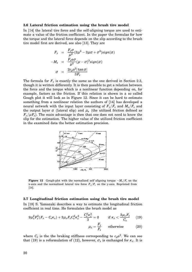
The formula for Fy is exactly the same as the one derived in Section 2.3,though it is written differently. It is then possible to get a relation betweenthe force and the torque which is a nonlinear function depending on, forexample, factors as the friction. If this relation is shown in a so calledGough plot it will look as in Figure 12. Since it can be hard to estimatesomething from a nonlinear relation the authors of [14] has developed aneural network with the input layer consisting of Fy/Fz and Mz/Fz andthe output layer α (lateral slip) and µu (the utilized friction defined asFy/µ Fz). The main advantage is then that one does not need to know theslip for the estimation. The higher value of the utilized friction coefficientin the examined data the better estimation precision.

Figure 12 Gough­plot with the normalized self aligning torque −Mz/Fz on thex­axis and the normalized lateral tire force Fy/Fz on the y­axis. Reprinted from[14].

3.7 Longitudinal friction estimation using the brush tire model

In [18] S. Yamazaki describes a way to estimate the longitudinal frictioncoefficient in real time. He formulates the brush model as

9µ2x F2

z (Fx − Csκ x) + 3µx FzC2s κ 2

x − C3s κ 3

x

3= 0 if κ x < 3µx Fz

Cs(19)

µx = Fx

Fzotherwise (20)

where Cs is the the braking stiffness corresponding to cpa2. We can seethat (19) is a reformulation of (12), however, σ x is exchanged for κ x. It is

20

not clear from the article how the estimation is performed. S. Yamazakijust claims that the friction coefficient can be easily obtained by solving(19). Measurements at two different surface conditions are performed ina drum type test machine. The measurement procedure started by havingthe drum and the test tire running at the same speed. Then a brakingtorque was slowly applied to the tire. The speed of the drum was heldconstant at 30 km/h. The tire will slow down and the slip velocity andthe corresponding braking force are measured. For the dry surface thecalculation of the friction coefficient seems to work well from 5 % slip andabove. For the wet condition the calculated friction value for slips belowthe limit in (19) has not been closer presented.

3.8 Friction estimation for vehicle path prediction

Vehicle path prediction is a method to either optimize the steering andbraking input to the vehicle for keeping a certain path or, at a fixed steeringinput, calculating when or if the vehicle will cross the outer borders of thepath[9]. For these calculations an accurate tire model is necessary. Whena tire develops a lateral force its longitudinal characteristics changes andthe brush model given in Section 2.3 is no longer valid. C. Liu and H. Pengmake the following simple extension of the brush model to take slip in twodimensions into account:

Fx,y = − kx,yσ x√

(kxσ x)2 + (kyσ y)2

(

3cσ − 31µ

(cσ )2

Fz+ 1

µ(cσ )3

F2z

)

(21)

where σ =√

σ 2x + σ 2

y and c, kx, ky are constants that relate to the tire

stiffnesses. The friction coefficient can then be calculated from the brakeforce and the slip, even though the tire is in a combined slip situation. Twoestimators to calculate the longitudinal force from the wheel speed andthe torque signals are proposed. One built on the recursive least squaresmethod and one is an enhanced adaptive observer. The bicycle model isused for the path prediction

d

dt

y

y

φ − φd

r

=

0 1 0 0

0 2 Cf +Cr

mu −2 Cf +Cr

mu 2 Cf a+Crb

mu

0 0 0 1

0 2 Cf a+Crb

mu−2 Cf a+Crb

mu2 Cf a2+Cr b2

mu

y

y

φ − φd

r

+

0

−2 Cf

m

0

−2 Cf a

Iz

δ f +

0

−u

−1

0

rd (22)

where r, φ , φd, y, v denote the yaw rate, the heading angle, the road head­ing angle, lateral displacement, and lateral velocity. From that the timeto lane crossing (TLC) can be predicted. The predicted path is continouslycompared to the real path to improve the values of the braking and corner­ing stiffnesses, Cf and Cr. In the model the lateral tire force is simplifiedto a linear function of the side slip. This will make the model only accu­rate at low lateral slip conditions and no longitudinal slip. The proposed

21

model predict a vehicle path at low slip conditions, but can also estimatethe friction coefficient at combined slip, so that a warning can be issued ifthe force at any tire is close to exceed its maximum limit.

3.9 Discussion

The general way to estimate the friction coefficient includes mainly twosteps. The first is to estimate the force working between the tire and theroad. The second is to have a model of the tire friction from which it ispossible to estimate µ when necessary signals are given.

There are mainly two systems from where the tire forces can be esti­mated or measured.

• The wheel. It has fast dynamic (high bandwidth) and is situated veryclose to the force generation point. The tire developers works withdifferent ways to measure the strain in the tire and from that derivethe forces. There also exists equipment for torque measurement onthe rim, but then the inertia of the wheel must be considered andknown. Finding out the tire forces from the wheel would be mostaccurate method.

• The vehicle. It has slow dynamics and the connection to the forcegeneration point is elastic.

Some of the friction estimation methods above need a good slip­signal.That could be a problem while the wheel speed for each wheel and thevelocity of the vehicle have to be known. All noise and bias on the wheelsensor signal are strongly amplified in the slip calculation. The quickerfilter the more necessary it is to have good measurements.

4. Changes to the Brush Tire Model to Enhance

Friction Estimation

As seen in Section 3 the brush tire model presented in Section 2.3 is widelyused to estimate the friction coefficient between the tire and the road. Itis possible to derive the friction both from lateral and longitudinal pureforce and slip measurements. See for example Section 3.6 and 3.8. How­ever, for the lateral estimation case some kind of compensation for theflexible carcass has to be made, but no solution for that has been foundin the literature. There are mainly two parameters that decide the shapeof the force­slip curve generated by the brush tire method. First the tirebrake/cornering stiffness 2cpa2 and then the maximal friction force µ Fz.cp is the rubber shear stiffness per length unit which varies with, for ex­ample, the tire wear. 2a is the length of the contact patch between the tireand the ground, which depend mostly on the vertical load on the axle, asdiscussed in Section 2.1. The friction coefficient µ can vary fast if the vehi­cle suddenly crosses a patch of ice or runs into a different road foundation.The vertical force Fz on each wheel can also vary quickly according to theunevenness of the road. Fz will also depend on the actions of the vehicle,since the inertia forces from its movement are brought up by the wheels.The difference between Fz and the other parameters mentioned above isthat Fz is assumed to be measured and then can be treated as a known

22

constant in the estimation. However, the noise from the unevenness of theroad shape has to be reduced by a filter.

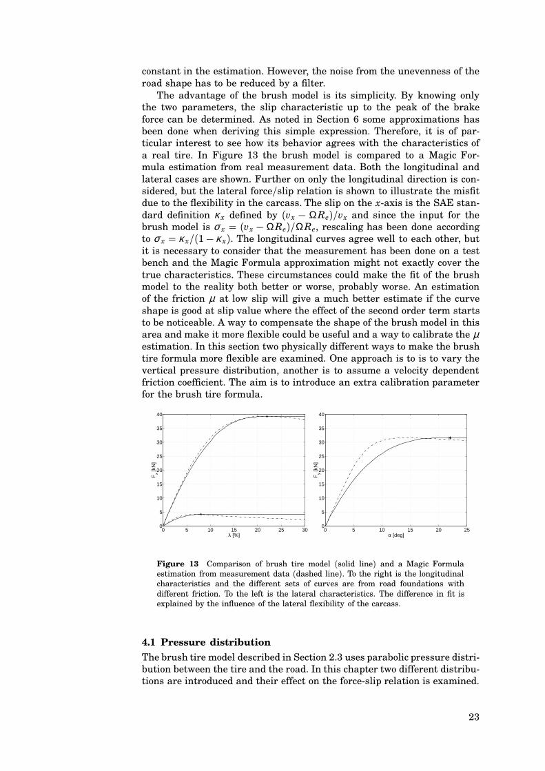
The advantage of the brush model is its simplicity. By knowing onlythe two parameters, the slip characteristic up to the peak of the brakeforce can be determined. As noted in Section 6 some approximations hasbeen done when deriving this simple expression. Therefore, it is of par­ticular interest to see how its behavior agrees with the characteristics ofa real tire. In Figure 13 the brush model is compared to a Magic For­mula estimation from real measurement data. Both the longitudinal andlateral cases are shown. Further on only the longitudinal direction is con­sidered, but the lateral force/slip relation is shown to illustrate the misfitdue to the flexibility in the carcass. The slip on the x­axis is the SAE stan­dard definition κ x defined by (vx − ΩRe)/vx and since the input for thebrush model is σ x = (vx − ΩRe)/ΩRe, rescaling has been done accordingto σ x = κ x/(1 − κ x). The longitudinal curves agree well to each other, butit is necessary to consider that the measurement has been done on a testbench and the Magic Formula approximation might not exactly cover thetrue characteristics. These circumstances could make the fit of the brushmodel to the reality both better or worse, probably worse. An estimationof the friction µ at low slip will give a much better estimate if the curveshape is good at slip value where the effect of the second order term startsto be noticeable. A way to compensate the shape of the brush model in thisarea and make it more flexible could be useful and a way to calibrate the µestimation. In this section two physically different ways to make the brushtire formula more flexible are examined. One approach is to is to vary thevertical pressure distribution, another is to assume a velocity dependentfriction coefficient. The aim is to introduce an extra calibration parameterfor the brush tire formula.

0 5 10 15 20 25 300

5

10

15

20

25

30

35

40

λ [%]

Fx [k

N]

0 5 10 15 20 250

5

10

15

20

25

30

35

40

α [deg]

Fy [k

N]

Figure 13 Comparison of brush tire model (solid line) and a Magic Formulaestimation from measurement data (dashed line). To the right is the longitudinalcharacteristics and the different sets of curves are from road foundations withdifferent friction. To the left is the lateral characteristics. The difference in fit isexplained by the influence of the lateral flexibility of the carcass.

4.1 Pressure distribution

The brush tire model described in Section 2.3 uses parabolic pressure distri­bution between the tire and the road. In this chapter two different distribu­tions are introduced and their effect on the force­slip relation is examined.

23

The first proposal is an asymmetric third order approach with an extraparameter which moves the top of the curve and changes the asymmetricproperties. The second curve is symmetric and defined by a forth order for­mulation. All equations are scaled so that the resulting force will be equalto Fz. The distributions are only defined in the longitudinal direction andsupposed to be the average value of the distribution in the lateral direction.The parabolic pressure distribution used in Section 2.3 is given by

q1(x) = 3Fz

4a

(

1 − x2

a2

)

(23)

and the asymmetric distribution is

q2(x) = 3Fz

4a

(

1 −( x

a

)2)

(

1 + dx

a

)

(24)

The expression for the symmetric forth order pressure curve is

q3(x) = 5Fz

8a

(

1 − x4

a4

)

(25)

The curves are visualized in Figure 14. In (24) it possible to move the pointof the maximal pressure to the left or to the right by changing d. To avoidnegative pressure values inside the contact patch the parameter must stayin the range of hdh < 1. A discussion about the shape of the contact patchand the pressure distribution is performed in Section 2.1 and the specialcase with a circular patch as to the left in Figure 2 with a very small tran­sition region the lumped pressure distribution would have an elliptic shape(qz = k0

√

1 − (x/a)2). Allowing a larger transition region the curve closeto x = ±a will decrease. Probably, q1(x) then is a realistic assumption. Forthe second case in Section 2.1, where the contact patch is more rectangular,q3(x) is a better choice. For these static cases the vertical pressure may notexceed the tire pressure. When the wheel rolls the continuous deformationof the tire changes the pressure distribution. The damping together withthe mass forces increases the pressure at the leading side and decrease iton the trailing side. There might also be some effects from the centrifugalforces caused by the wheel rotation. The asymmetric third order function,q2(x), with a positive d is then a realistic choice. When a brake force isapplied the carcass is strained in the leading end and compressed in thetrailing end. This could have the effect of moving the center of the pressuredistribution backwards and the d could then reach a negative value. A cor­rect choice of pressure distribution needs a lot of further investigation andmeasurements. Later on we will see how different distributions affects theforce­slip curve and that the choice of it might not be done on theoreticalfoundations.

Force­slip function for an asymmetric pressure distribution. Curve1 in Figure 8 is now replaced by (24) and by eliminating the root xs = a

from (11) the breakaway point can be derived by

3 Fzµ4 a2

(

1 + x

a

) (

1 + dx

a

)

= cpσ x (26)

24

−1 −0.8 −0.6 −0.4 −0.2 0 0.2 0.4 0.6 0.8 10

0.1

0.2

0.3

0.4

0.5

0.6

0.7

0.8

0.9

1

Contact patch (a m)

Pre

ssur

e (

Fz/

a kN

/m)

d=−0.3 d=0.5

Figure 14 The pressure distributions proposed in this chapter. The wheel issupposed to move to the right. The leading side will then be to the right and thetrailing side is accordingly to the left. the solid line shows pressure distributionaccording to equation (23), dashed line according to equation (25) and the dasheddotted ones to equation (24) with different choices on d.

with the solutions

xs = − a

2d(d + 1) ± a

2d

√

(d − 1)2 + 16a2cpd

3µ Fzσ x (27)

To be able to use the calculation scheme from Section 2.3, one and only onesolution can be inside the contact region. Therefore the sign in front of thesquare root has to be positive. For d less than −0.5 there are two solutionsinside the interval. Physically it means that there are two sliding areassplit by one adhesive region. To avoid that, the interval for d is restrictedto [−0.5, 1]. The total brake force, which is illustrated by the marked areain Figure 8, is described by the integral

Fx =∫ xs

−a

3µ Fz

4a

(

1 −( x

a

)2)

(

1 + dx

a

)

dx+∫ a

xs

(a − x)cpσ x dx (28)

which gives the following expression

Fx = µ Fz

32d3 (1 − d)3(3d + 1) + cp a2

4 d2 (2 d + 5 d2 + 1)σ x

+ 13

c2p a4 σ 2

x

µ Fz d−

(

µ Fz

32d3 (d − 1)2 + cp a2

6 d2

)

(3 d + 1)σ x

⋅

√

(d − 1)2 + 16 d cp σ x a2

3µ Fz

(29)

25

The slip limit where the entire contact area slides towards the ground isgiven by the incline of the pressure curve in x = a. Hence,

Fx = µ Fz if σ x > 3µ Fz

2cpa2 (1 + d) (30)

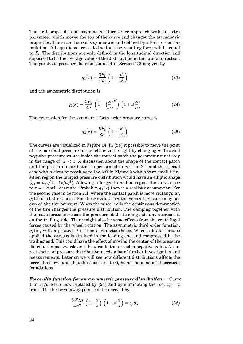
The result for some different values of d is shown in Figure 15. The com­plexity of (29) could be reduced by choosing d to 1 or −1/3. However, theidea to change the pressure distribution in this way is to get a calibrationparameter that can be changed continuously.

0 0.05 0.1 0.15 0.2 0.25 0.30

0.2

0.4

0.6

0.8

1

Slip

Nor

mal

ized

Bra

ke F

orce

d=−0.2, 0, 0.3, 0.5

Figure 15 Illustration showing the brake force contra the slip using the pressuredistribution given by (24). The solid line denotes a Magic Formula realization froma real tire. The others are derived using different value of d.

Symmetric fourth order pressure distribution The same procedureas above can be done for the pressure distribution described by (25). Thereis no extra parameter introduced in this approach and yet the expressionfor the solution gets too complex to be presented. The shape of the resultingforce­slip curve, which is shown in Figure 16, shows the difference usingthe fourth order distribution.

Discussion The results from the alternative brush models have so faronly been compared to one Magic Formula estimation. The Magic Formulahas got a lot of acceptance and is the best way to approximate measurementdata by an expression. However, it might not be the entire truth. Therefore,it could be dangerous to draw too many conclusions just from this referencecurve. There are also other factors than the pressure distribution that canaffect the shape of the curve. Having that in mind we say that the fourthorder curve matches very well at slip up to 70% of the maximal brakeforce. This means that the distribution is realistic at the trailing side,but the pressure should decrease faster when reaching the leading end.The parabolic pressure distribution give a good overall fit to the MagicFormula approximation. However, choosing the asymmetric curve with a

26

0 0.05 0.1 0.15 0.2 0.25 0.30

0.2

0.4

0.6

0.8

1

Slip

Nor

mal

ized

Bra

king

For

ce

Figure 16 Brake force contra slip. The solid line denotes a Magic Formula op­timized from real data. The dashed line is derived form the fourth order pressuredistribution and the dashed­dotted from the non­compensated brush model derivedin Section 2.3.

slightly negative d gives better accuracy for slip up to 0.07, even thoughit has some mismatch at higher brake forces. That implies that the topof the pressure distribution should be a little bit behind the the centerof the contact patch. It could also imply that d and the peak moves withthe achieved brake force, which is reasonable. Then the d­value should bechanged depending on the load and brake force.

4.2 Velocity dependent friction

Another way to increase the flexibility of the brush tire model is to in­troduce a sliding­velocity dependent friction coefficient. The bristles inthe contact patch are assumed to slide against the road with the veloc­ity vsx = vxσ x/(σ x + 1) directly after passing the breakaway point xs, seeFigure 8.

Three different cases of velocity dependence are treated in the following.First, in the meaning that the friction is constant but has different valuewhether the bristles are gripping or sliding on the road. The value µs de­notes the static friction and µk, the kinetik. In the second case the frictioncoefficient is linearly dependent on the sliding velocity. Finally, an expo­nential relation between the friction and the sliding velocity is assumed.The two last cases are examined in two ways. Either, only the kinetic fric­tion will be velocity dependent and the static coefficient constant or boththe static and the kinetic friction have the same velocity dependence.

Constant friction The friction is in this case assumed to be constant,but having different values whether the bristles are sliding or gripping theroad. Referring back to Section 2.3 and solving Equation (8) gives the pointin the contact patch where sliding starts as

xs = 13

a (4 cpσ x a2 − 3 µs Fz)µs Fz

27

Evaluating (9) where µ is changed to µk gives

Fx = 2 cp a2 σ x + 43

c2p a4 (µk − 2 µs)σ 2

x

Fz µ2s

+ 827

c3p a6 (3 µs − 2 µk)σ 3

x

F2z µ3

s

(31)

For σ x > 3µs Fz/(2cp a2) the entire surface slides and the brake force isgiven by

Fx = µk Fz

A difference between this realization and the one from Section 2.3 is thatthe top of brake force curve is reached for a lower slip than total slidingoccurs. By differentiating (31) and locating the zeros the slip value thatcorresponds to the peak force can be derived. Since (31) is a third orderequation two zeros are obtained. One belonging to the maximal force andone belonging to the slip where the total sliding starts, the same point asmentioned above. The slip, where the force has its maximum, is given by

σ = 3µ2s Fz

2cpa2 (3µs − 2µk) (32)

and the peak force is

Fmax = (4µs − 3µk)µ2s

(3µs − 2µk)2 Fz (33)

The calibration factor m is introduced such that the shape of the force/slipcurve can be adjusted for given braking stiffness and peak brake force.Define m = µk/µs and the static friction can be expressed by µs = Fmax(3−2m)2/(Fz(4−3m)) for m ∈ [0, 1] . In Figure 17 the force­slip curve is plottedfor some different values of m. The expression for the force including theparameter m and µ ′ = Fmax/Fz, for σ x ≤ 3µs/(2cpa2) is

Fx = 2 cp a2 σ x + 43

c2p a4 (m − 2)

Fzµ ′(4 − 3m)(3 − 2m)2 σ 2

x + 827

c3p a6

(Fz µ ′)2

(4 − 3m)2

(3 − 2m)3 σ 3x

(34)

Linear velocity dependency To include velocity dependence on thefriction, any relation µk = fk(vs) and µs = fs(vs) can be put into (31).µ = f (vs) can be put into (12) if both friction coefficients are assumed todepend on the slip velocity in the same way. Recall that vs is the relativevelocity between the tire carcass and the road. The entire sliding part inthe contact patch is assumed to slide with vs. Since the work is restrictedto only longitudinal movements vs = vsx and the velocity of the vehiclev=vx. vsx can be expressed as κ xvx according to the table in Section 2.2.The expressions have to be dependent on σ x instead of κ x so the followingtransform vsx = vxσ x/(1 + σ x) is done. With constant static friction thefollowing expression is used for the kinetic friction.

µk(σ x, v) = µ0 − n vσ x

1 + σ x

(35)

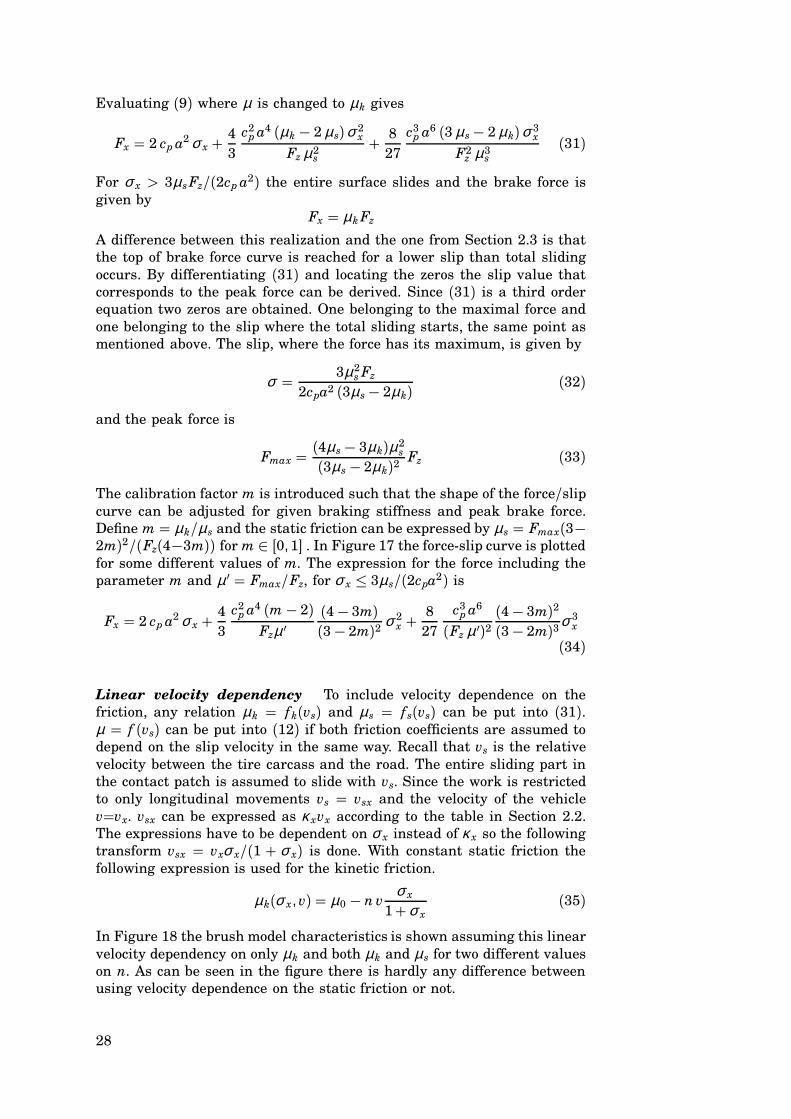
In Figure 18 the brush model characteristics is shown assuming this linearvelocity dependency on only µk and both µk and µs for two different valueson n. As can be seen in the figure there is hardly any difference betweenusing velocity dependence on the static friction or not.

28

0 0.05 0.1 0.15 0.2 0.25 0.3 0.35 0.40

0.2

0.4

0.6

0.8

1

slip

Nor

mal

ized

Bra

ke F

orce

Figure 17 The figure shows the force­slip curve derived by the brush tire modelwith different friction value for adhesive and sliding areas. Solid line is the MagicFormula estimated from real data. Dashed dotted curve has m = 1 and dasheddotted lines has m equal to 0.6 and 0.8.

0 0.1 0.2 0.3 0.4 0.50

0.2

0.4

0.6

0.8

1

Slip

Nor

mal

ized

Bra

ke F

orce

0 0.1 0.2 0.3 0.4 0.50

0.2

0.4

0.6

0.8

1

Slip

Nor

mal

ized

Bra

ke F

orce

Figure 18 The left figure shows the force­slip relation with linear velocity de­pendence. Solid line is the magic formula estimated from real data. The dashedcurve has µ0 = 1.05 and n = 0.0075 and the dashed dotted curve has µ0 = 1.05and n = 0.0075. Both the case with µs = µ0 and µs = µk is plot, but the differenceis hardly noticeable. To the right exponential velocity dependence is plotted forµ = 1.3 and h = 0.4. For the dashed dotted line µs = µ0 = µk(0) and the dashedµs = µk(vs),

Exponential velocity dependency For exponential velocity dependencethe following relation, which also is proposed by C. Canudas de Wit in [4],is used

µk(σ x, v) = µc + (µs − µc)e−hvσ x/((1+σ x)vst)hε (36)

Four parameters are necessary to describe this relation. It gives good flexi­bility and the brush model can almost be adjusted to fit any Magic Formulaset. Clearly, the aim to introduce one calibration parameter is then not ful­filled and the number of parameters has to be reduced. The reduction canbe done by fixing some of parameter values. In Figure 18 ε = 0.5 and

29

vst = 30 m/s and the calibration parameter h is introduced as

µk(σ x, v) = µ(

h + (1 − h)e−hvσ x/((1+σ x)30)h0.5)

(37)

The right illustration in Figure 18 shows that the difference betweenthe adhesive and the sliding friction gives a sharp hook on the force slipcurve just before entering the slip for total sliding. When studying rawdata from tests of tires this fenomenon is often observed, but it is notreally covered by the Magic Formula parameterization.

Discussion From the result in this section it can be seen that it is onlypossible to change the slope of the brush tire model curve at slip valuesclose to or above the point for total sliding when using velocity dependencefor calibration. This is obvious considering the fact the larger slip the largershare of the brake force is depending on the friction characteristic.

In the literature it has been shown that even the adhesive friction coef­ficient can be depending on the speed that pulls the materials away formits original position. Assuming the case with different static and kineticfriction gives too negative slope behind the maximal force point. This couldmaybe be changed by a combination of velocity dependent friction and an­other pressure distribution then the parabolic one. The great advantage ifone could get these approximation more realistic is that it would be pos­sible to prescribe the negative slope without or just before entering thatzone.

4.3 Taylor expansion

Estimation of parameters using schemes as the least squares method arefacilitated by use of a simple expression. Therefore, a polynomial approx­imation for the expression above with parameters depending on d, m, n,or h is performed. In this section the expressions are simplified by Taylorexpansion.

Taylor expansion of the expression for the asymmetric pressure

distribution Expanding (29) in a Taylor series, with d in the interval−0.5 < d < 1, gives the following expression:

Fx = 2 cp a2 σ x + 43

c2p a4

(d − 1) µ Fzσ 2

x − 827

(3 d + 1) cp3 a6

(d − 1)3 µ2 Fz2 σ 3

x

+ 1627

(3 d + 1) cp4 a8 d

(d − 1)5 Fz3 u3

σ 4x − 128

81(3 d + 1) cp

5 a10 d2

(d − 1)7 Fz4 u4

σ 5x + O(σ 6

x) (38)

When truncating a series expansion there is alway a question about theconvergence. In this case it is no restriction to a certain number of terms,but the advantage of the Taylor expansion gets lost if the convergenceis slow. If d = −1/3 and 0, only 2 respectively 3 terms are needed todeliver exact convergence. For d < 0.1 sufficient accuracy is reached usingfour terms. At this point “sufficient accuracy” is somewhat diffuse. Theestimation scheme has to be set before a distinct demand an the accuracycan be determined. For higher values it is more critical and more terms areneeded. Of course the convergence also depends on the value of cpa2/µ Fz .The correct expression together with Taylor expansion truncated after thethree respective four terms are shown in Figure 19.

30

0 0.05 0.1 0.15 0.2 0.25 0.30

0.2

0.4

0.6

0.8

1

slip

Nor

mal

ized

Bra

ke F

orce

0 0.05 0.1 0.15 0.2 0.25 0.30

0.2

0.4

0.6

0.8

1

slip

Nor

mal

ized

Bra

ke F

orce

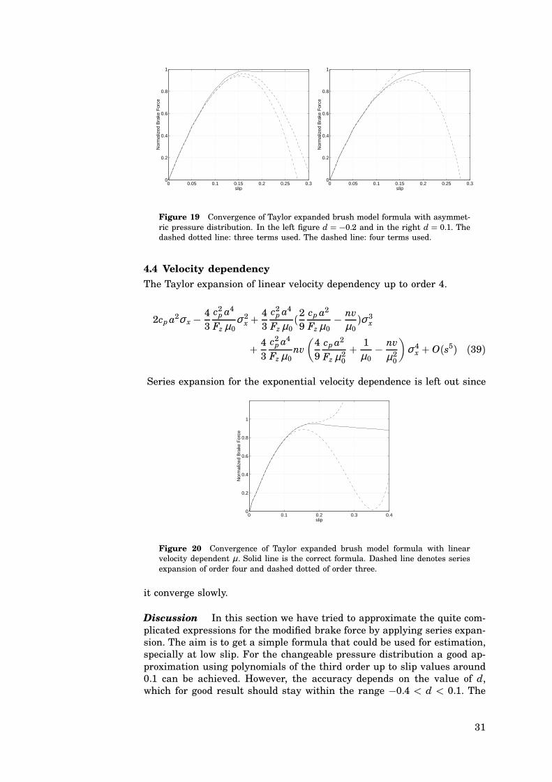
Figure 19 Convergence of Taylor expanded brush model formula with asymmet­ric pressure distribution. In the left figure d = −0.2 and in the right d = 0.1. Thedashed dotted line: three terms used. The dashed line: four terms used.

4.4 Velocity dependency

The Taylor expansion of linear velocity dependency up to order 4.

2cp a2σ x − 43

c2p a4

Fz µ0σ 2

x + 43

c2p a4

Fz µ0(29

cp a2

Fz µ0− nv

µ0)σ 3

x

+ 43

c2p a4

Fz µ0nv

(

49

cp a2

Fz µ20

+ 1µ0

− nv

µ20

)

σ 4x + O(s5) (39)

Series expansion for the exponential velocity dependence is left out since

0 0.1 0.2 0.3 0.40

0.2

0.4

0.6

0.8

1

slip

Nor

mal

ized

Bra

ke F

orce

Figure 20 Convergence of Taylor expanded brush model formula with linearvelocity dependent µ . Solid line is the correct formula. Dashed line denotes seriesexpansion of order four and dashed dotted of order three.

it converge slowly.

Discussion In this section we have tried to approximate the quite com­plicated expressions for the modified brake force by applying series expan­sion. The aim is to get a simple formula that could be used for estimation,specially at low slip. For the changeable pressure distribution a good ap­proximation using polynomials of the third order up to slip values around0.1 can be achieved. However, the accuracy depends on the value of d,which for good result should stay within the range −0.4 < d < 0.1. The

31

case where the friction depends linearly with the velocity the approxima­tion also shows a good result. for the exponential dependency it seemsmore difficult to approximate the derived formula by a series expansion.The convergence is not enough.

5. Simulation of Friction Estimation with Brush

Model

The aim for the simulation in this section is to examine the possibility ofestimating the friction between the tire and the road, without reaching thepeak force point. The brush model explained in Section 2.3 is used, since thefriction coefficient is explicitly included in the derived expression. Finally,there is a brief discussion of how different choices of the calibration factord affects the estimates.

5.1 Data generation

The model for the data generation is built in Simulink and describes awheel with a certain inertia. A torque can be applied to the wheel rimwhich through the tire develops a brake force. The brake force causes avelocity difference (slip) between the road and the wheel with a relationdescribed by the Magic Formula:

Fx = FzD sin (C arctan (Bκ x − E(Bκ x − arctanBκ x))) (40)

where the coefficients B, C, D, E have been estimated from test data. Theset of coefficients used here characterize a normal tire, having a stiffnessCx = 5e5, running on asphalt, with µ = 0.98. On the signals necessary forthe estimation noise is added with the covariances σ 2

λ = 0.2 ⋅ 10−4 on theslip and σ 2

Fx= 0.2 ⋅ 10−2 F2

z on the force signal. Vehicle tests performed ata Scania truck have shown these values to be realistic. Fz is considered asa constant. The simulated data is generated by application of the torquein a saw tooth like manner to the wheel rim with the aim to reproduce thetorque ramp that arises when the brakes are applied in a braking situation.Different amplitudes of the input signals are tested. The normalized brakeforce for a input signal of amplitude of 75% of the peak force is shown inFigure 21.

5.2 Estimation of brush model parameters

The expression for the brake force as a function of the slip using the brushtire model with the proposed calibration factor d is

Fx = Cx σ x + 13

C2x

(d − 1) µ Fzσ 2

x − 127

(3 d + 1) C3x

µ2 Fz2(d − 1)3

σ 3x (41)

The included coefficients are further presented in Section 2.3 and the re­lation between σ x and λ is given by σ x = λ/(1 − λ). The brush model canbe parameterized as

y = θ0u0 + θ1u1 + θ2u2 + e (42)

32

0 0.5 1 1.5 2 2.5 3 3.5 40

0.1

0.2

0.3

0.4

0.5

0.6

0.7

0.8

Time (sec)

Nor

mal

ized

bra

ke fo

rce

0 0.01 0.02 0.03 0.04 0.05 0.06 0.07 0.08 0.09 0.10

0.1

0.2

0.3

0.4

0.5

0.6

0.7

0.8

Slip

Nor

mal

ized

bra

ke fo

rce

Figure 21 To the left the input signal is shown as the normalized brake forcewhich actually is direct proportional the input torque. To the right the same signalis shown as a function of the generated slip.

with the following regressors

y = Fx

Fz(43)

u0 = Cx0σ x (44)

u1 = − 13µ0

(Cx0σ x)2

Fz(45)

u2 = 127µ2

0

(Cx0σ )3

F2z

3d + 1(d − 1)3 = u2

1

3 u0

3d + 1d − 1

(46)

The tire parameters of interest can be derived as

Cx = θ0Cx0 (47)

µ = θ 20

θ1µ0 (48)

Then the third parameter θ2 can be expressed by the other two parametersθ0 and θ1 as θ2 = θ 2

1/θ0 and (42) can be rewritten in the following form

y = θ0u0 + θ1u1 + θ 21

θ0

u21

3 u0

3d + 1d − 1

+ e (49)

Two different estimation procedures are compared, the recursive leastsquares (RLS) algorithm with forgetting factor and the MIT­rule. The well­known RLS described in for example [8] works only with linear equationsand the nonlinear factor has to be treated separately. Here it is includedin the output signal as

y′(k) = y(k) − θ 21(k − 1)

θ0(k − 1)u2(k) (50)

and the following linear expression,

y′(k) = θ0(k)u0(k) + θ1(k)u1(k) + e(k) (51)

33

can be used for update of the θ ­parameters.The MIT­rule [1] treats the nonlinearity and to update each parameter

the formula

dθ i = −γ eV e

Vθ i(52)

is used and e and its partial derivatives can be derived from (49).

5.3 Estimation results

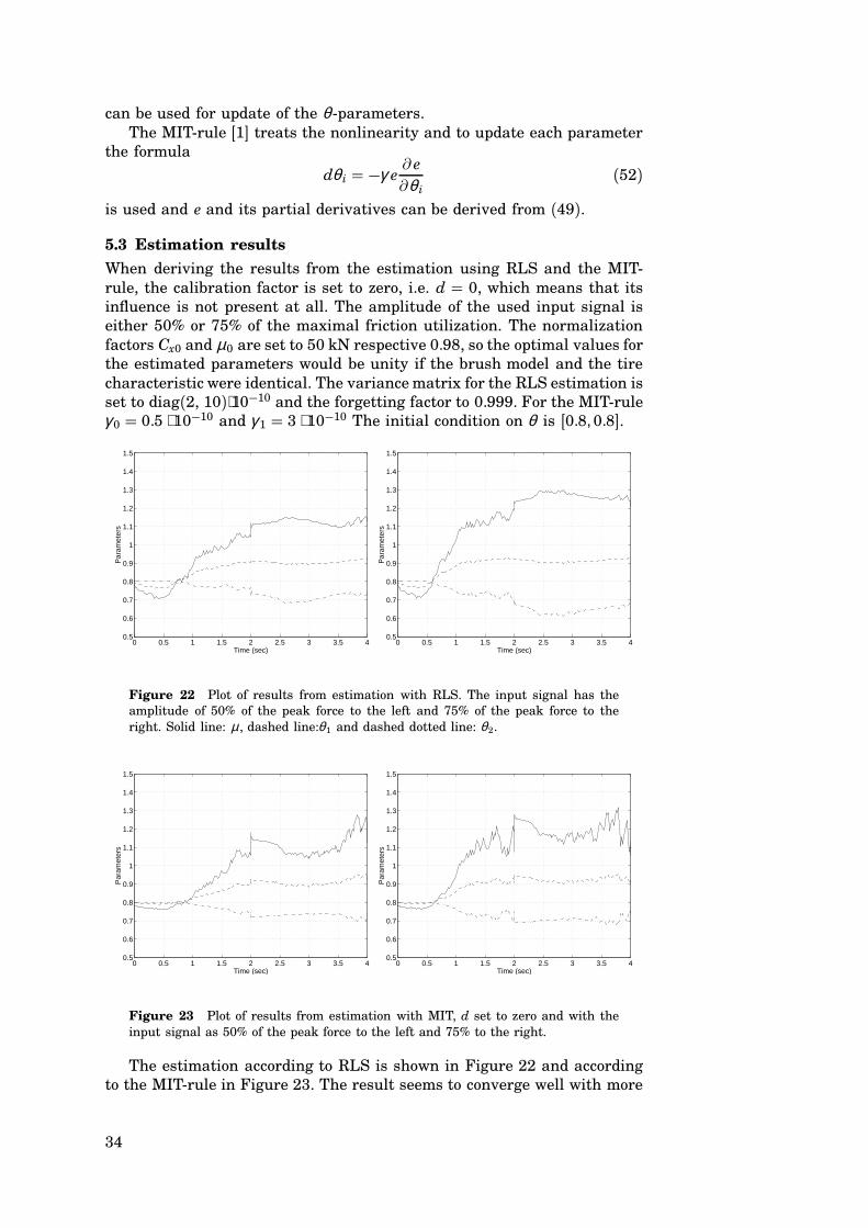
When deriving the results from the estimation using RLS and the MIT­rule, the calibration factor is set to zero, i.e. d = 0, which means that itsinfluence is not present at all. The amplitude of the used input signal iseither 50% or 75% of the maximal friction utilization. The normalizationfactors Cx0 and µ0 are set to 50 kN respective 0.98, so the optimal values forthe estimated parameters would be unity if the brush model and the tirecharacteristic were identical. The variance matrix for the RLS estimation isset to diag(2, 10)⋅10−10 and the forgetting factor to 0.999. For the MIT­ruleγ 0 = 0.5 ⋅ 10−10 and γ 1 = 3 ⋅ 10−10 The initial condition on θ is [0.8, 0.8].

0 0.5 1 1.5 2 2.5 3 3.5 40.5

0.6

0.7

0.8

0.9

1

1.1

1.2

1.3

1.4

1.5

Time (sec)

Par

amet

ers

0 0.5 1 1.5 2 2.5 3 3.5 40.5

0.6

0.7

0.8

0.9

1

1.1

1.2

1.3

1.4

1.5

Time (sec)

Par

amet

ers

Figure 22 Plot of results from estimation with RLS. The input signal has theamplitude of 50% of the peak force to the left and 75% of the peak force to theright. Solid line: µ , dashed line:θ1 and dashed dotted line: θ2.

0 0.5 1 1.5 2 2.5 3 3.5 40.5

0.6

0.7

0.8

0.9

1

1.1

1.2

1.3

1.4

1.5

Time (sec)

Par

amet

ers

0 0.5 1 1.5 2 2.5 3 3.5 40.5

0.6

0.7

0.8

0.9

1

1.1

1.2

1.3

1.4

1.5

Time (sec)

Par

amet

ers

Figure 23 Plot of results from estimation with MIT, d set to zero and with theinput signal as 50% of the peak force to the left and 75% to the right.

The estimation according to RLS is shown in Figure 22 and accordingto the MIT­rule in Figure 23. The result seems to converge well with more

34

0 1 2 3 40

0.1

0.2

0.3

0.4

0.5

0.6

0.7

0.8

0.9

1

1.1

1.2

1.3

1.4

1.5

Time (sec)

Par

amet

er (µ

)

0 1 2 3 40

0.1

0.2

0.3

0.4

0.5

0.6

0.7

0.8

0.9

1

1.1

1.2

1.3

1.4

1.5

Time (sec)

Par

amet

er (µ

)

Figure 24 Illustration of the difference between the estimation of two differenttires with different friction. To the left the input signal is 50 % of the peak forcefor the original tire and to the right the input signal is 75 %. Solid line denotes thetire previously used the dashed line denotes the new one.

accurate estimate for the lower input signal in both cases. This was not asexpected and it was found out that the initial conditions together with theupdate speed of θ1 are very important for the estimation result, speciallyfor the lower force case. In reality most often the parameters are more orless known and the initial values not need to differ much the real values,but changes has to be detected. Therefore an additional estimation wasperformed on an tire with less friction. The result is shown in Figure 24.Since the friction coefficient was lower the input signal now reached 56%and 85% of the brake force peak for the same amplitude that was usedfor the first tire. The result clearly shows that friction estimation with thebrush model is possible, at least to discover changes. The bias in the finalestimate hopefully can be reduced by better adjustment of updating. Alsothe irregularity in the estimation at the time t = 2 s, when the input signalgets down to zero requires further work on the algorithm. Once again itmust be pointed out that real tire data was used, but it came from labo­ratoral environment and implementation in reality can differ significantly.The described method to introduce calibration factors is one attempt tocover for this uncertainty.

5.4 Effect of the calibrating d­factor

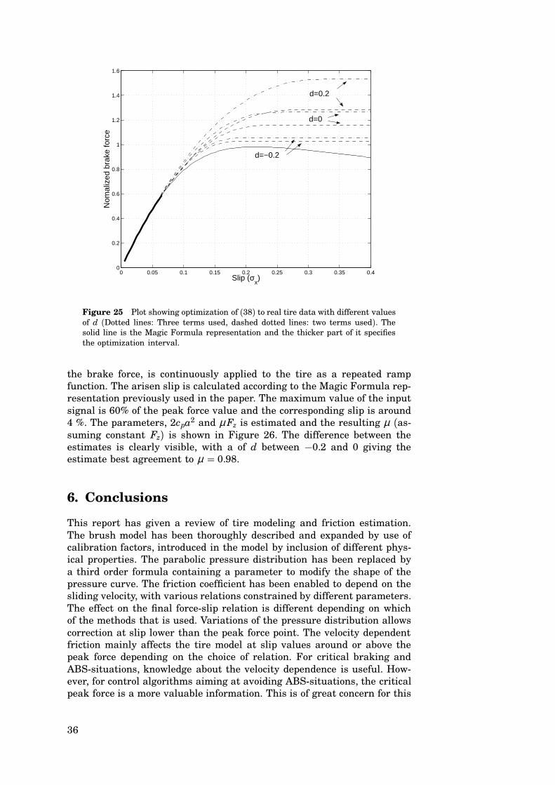
To verify and examine the function of the calibration factor introduced inSection 4 and the accuracy of the Taylor expansion, an optimization wasperformed. The parameters, θ1 = cpa2 and θ2 = µ Fz, included in (38) werechosen to minimize the error between the brush model curve and the realtire data for forces up to 60% of the peak value and with different valueon d. The optimization was done for two or three terms. In Figure 25 theresults for the obtained parameter values inserted in (29) are shown. Itclearly shows the difference when using two or three terms for the opti­mization. By using a correct calibration factor the effect of the truncationcan be diminished and an accurate estimation can be achieved for fewterms.

Since two terms seem to give accuracy enough for low slip, on­line fric­tion estimation using the recursive least squares method might be per­formed. This has been verified by simulations, where the input signal, i.e.

35

0 0.05 0.1 0.15 0.2 0.25 0.3 0.35 0.40

0.2

0.4

0.6

0.8

1

1.2

1.4

1.6

d=−0.2

d=0

d=0.2

Slip (σx)

Nom

aliz

ed b

rake

forc

e

Figure 25 Plot showing optimization of (38) to real tire data with different valuesof d (Dotted lines: Three terms used, dashed dotted lines: two terms used). Thesolid line is the Magic Formula representation and the thicker part of it specifiesthe optimization interval.

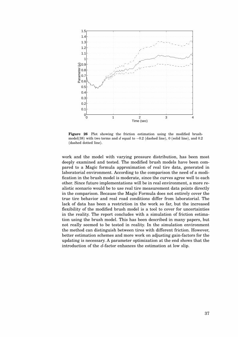
the brake force, is continuously applied to the tire as a repeated rampfunction. The arisen slip is calculated according to the Magic Formula rep­resentation previously used in the paper. The maximum value of the inputsignal is 60% of the peak force value and the corresponding slip is around4 %. The parameters, 2cpa2 and µ Fz is estimated and the resulting µ (as­suming constant Fz) is shown in Figure 26. The difference between theestimates is clearly visible, with a of d between −0.2 and 0 giving theestimate best agreement to µ = 0.98.

6. Conclusions

This report has given a review of tire modeling and friction estimation.The brush model has been thoroughly described and expanded by use ofcalibration factors, introduced in the model by inclusion of different phys­ical properties. The parabolic pressure distribution has been replaced bya third order formula containing a parameter to modify the shape of thepressure curve. The friction coefficient has been enabled to depend on thesliding velocity, with various relations constrained by different parameters.The effect on the final force­slip relation is different depending on whichof the methods that is used. Variations of the pressure distribution allowscorrection at slip lower than the peak force point. The velocity dependentfriction mainly affects the tire model at slip values around or above thepeak force depending on the choice of relation. For critical braking andABS­situations, knowledge about the velocity dependence is useful. How­ever, for control algorithms aiming at avoiding ABS­situations, the criticalpeak force is a more valuable information. This is of great concern for this

36

0 1 2 3 40

0.1

0.2

0.3

0.4

0.5

0.6

0.7

0.8

0.9

1

1.1

1.2

1.3

1.4

1.5

Time (sec)

Par

amet

er (µ

)

Figure 26 Plot showing the friction estimation using the modified brush­model(38) with two terms and d equal to −0.2 (dashed line), 0 (solid line), and 0.2(dashed dotted line).

work and the model with varying pressure distribution, has been mostdeeply examined and tested. The modified brush models have been com­pared to a Magic formula approximation of real tire data, generated inlaboratorial environment. According to the comparison the need of a modi­fication in the brush model is moderate, since the curves agree well to eachother. Since future implementations will be in real environment, a more re­alistic scenario would be to use real tire measurement data points directlyin the comparison. Because the Magic Formula does not entirely cover thetrue tire behavior and real road conditions differ from laboratorial. Thelack of data has been a restriction in the work so far, but the increasedflexibility of the modified brush model is a tool to cover for uncertaintiesin the reality. The report concludes with a simulation of friction estima­tion using the brush model. This has been described in many papers, butnot really seemed to be tested in reality. In the simulation environmentthe method can distinguish between tires with different friction. However,better estimation schemes and more work on adjusting gain­factors for theupdating is necessary. A parameter optimization at the end shows that theintroduction of the d­factor enhances the estimation at low slip.

37

7. References

[1] K. J. Åström and B. Wittenmark. Adaptiv Control. Addison­WesleyPub Co, 1994.

[2] E. Bakker, H.B. Pacejka, and L. Lidner. A new tire model with anapplication in vehicle dynamics studies. SAE 890087, 1989.

[3] Carlos Canudas de Wit and Panagiotis Tsiotras. Dynamic tire frictionmodels for vehicle traction control. In Proceedings of the 38th IEEE

Conference on Decision and Control, volume 4, pages 3746–3751, 1999.

[4] Carlos Canudas de Wit, Panagiotis Tsiotras, and Xavier Claeys.Friction tire/road modeling, estimation and optimal braking control.In Lund NACO2 Workshop, 2001.

[5] M. Gäfvert and J. Svendenius. Construction of semi empirical tiremodels for combined slip. Technical Report ISRN LUTFD2/TFRT—7606–SE, Department of Automatic Control, LTH, Sweden, May 2003.

[6] Fredrik Gustafsson. Slip­based tire­road friction estimation. Automat­

ica, 33(6):1087–1099, 1997.

[7] Jin­Oh Hahn, Rajesh Rajamani, and Lee Alexander. Gps­based real­time identification of tire­road friction coefficient. IEEE Transactions

on Control Systems Technology, 10(3):331–343, May 2002.

[8] Rolf Johansson. System Modeling and Identification. Prentice Hall,2002.

[9] C.­S. Liu and H. Peng. Road friction coefficient estimation for vehiclepath prediction. Vehicle system Dynamics, 25:413–425, 1996.

[10] Stefan Muller and Michael Uchanski. Slip­based tire­road frictionestimation during braking. In Proceedings of IMECE01. ASME, 2001.

[11] Olle Nordström. Antilås system för tungafordon, VTI Rapport nr 257.Klintland grafiska, 1983.

[12] Eiichi Ono, Katsuhira Asano, and Masaru Sugai. Estimation ofautomotive tire force characteristics using wheel velocity. In IFAC

Triennial World congress, volume 15, 2002.

[13] H.B. Pacejka. Modeling of the Pneumatic Tyre and its Impact on

Vehicle Dynamic Behavior. Delft, Delft, 1988.

[14] W. R. Pasterkamp and H. B. Pacejka. The tyre as a sensor to estimatefriction. Vehicle System Dynamics, 27, 1997.

[15] J.P. Pauwelussen, Gabriel Anghelache, Claudiu Theodorescu, andA. Schmeitz. European Tire School, chapter Module 10 ­ Truck tyrebehavior in use and testing methods.

[16] Laura Ray. Nonlinear tire force estimation and road friction identi­fication: Simulation and experiments. Automatica, 33(10):1819–1833,1997.

[17] J. Y. Wong. Theory of Ground Vehicles. Number ISBN 0­471­35461­9.John Wiley & Sons, Inc., 2001.

[18] S. Yamazaki, O. Furukawa, and T. Suzuki. Study on real timeestimation of tire to road friction. Vehicle System Dynamics, 27, 1997.

38