reviewing inferential statistics

1

Reviewing Inferential Statistics

IntroductionNormal DistributionsSampling: The Case of AIDSEstimationStatistics in Practice: The War on DrugsBox 1. Interval Estimation for Peers as a Major Influence

on the Drug Attitudes of the YoungThe Process of Statistical Hypothesis Testing

Step 1: Making AssumptionsStep 2: Stating the Research and Null Hypotheses and Selecting Alpha

Box 2. Possible Hypotheses for Comparing Two SamplesStep 3: Selecting a Sampling Distribution and a Test Statistic

Box 3. Criteria for Statistical Tests When Comparing Two SamplesStep 4: Computing the Test Statistic

Box 4. Formulas for t, Z, and χ2

Step 5: Making a Decision and Interpreting the ResultsStatistics in Practice: Education and Employment

Sampling Technique and Sample CharacteristicsComparing Ratings of the Major Between Sociology

and Other Social Science AlumniRatings of Foundational Skills in Sociology: Changes over Time

Box 5. Education and Employment: The Process of Statistical Hypothesis Testing, Using Chi-Square

Gender Differences in Ratings of Foundational Skills, Occupational Prestige, and Income

Box 6. Occupational Prestige of Male and Female Sociology Alumni: Another Example Using a t TestConclusion

SPSS DemonstrationSPSS Problems Chapter Exercises

Source: Social Statistics for a Diverse Society, Third Edition by Chava Frankfort-Nachmias and Anna Leon-Guerrero. Copyright © 2002 by SAGE.

Reviewing Inferential Statistics2

22 Introduction

The goal of this online chapter is to provide a concise summary of inferential statistics. Remember that it is a concise summary and it is not all-inclusive.

22 Normal Distributions

The normal distribution is central to the theory of inferential statistics. This theoretical distribution is bell-shaped and symmetrical, with the mean, the median, and the mode all coinciding at its peak and frequencies gradually decreasing at both ends of the curve. In a normal distribution, a constant proportion of the area under the curve lies between the mean and any given distance from the mean when measured in standard deviation units.

Although empirical distributions never perfectly match the ideal normal distribution, many are near normal. When a distribution is near normal and the mean and the standard deviation are known, the normal distribution can be used to determine the frequency of any score in the distribution regardless of the variable being analyzed. But to use the nor-mal distribution to determine the frequency of a score, the raw score must first be converted to a standard or Z score. A Z score is used to determine how many standard deviations a raw score is above or below the mean. The formula for transforming a raw score into a Z score is

ZY Y

SY

= −

where

Y = the raw score

Y = the mean score of the distributionS

Y = the standard deviation of the distribution

A normal distribution expressed in Z scores is called a standard normal distribution and has a mean of 0.0 and a standard deviation of 1.0.

The standard normal curve allows researchers to describe many characteristics of any distribution that is near nor-mal. For example, researchers can find

•• The area between the mean and a specified positive or negative Z score

•• The area between any two Z scores

•• The area above a positive Z score or below a negative Z score

•• A raw score bounding an area above or below it

•• The percentile rank of a score higher or lower than the mean

•• The raw score associated with any percentile

The standard normal curve can also be used to make inferences about population parameters using sample statis-tics. Later we will review how Z scores are used in the process of estimation and how the standard normal distribution can be used to test for differences between means or proportions (Z tests). But first let’s review the aims of sampling and the importance of correctly choosing a sample.

1 This chapter was coauthored with Pat Pawasarat.

3Reviewing Inferential Statistics

22 Sampling: The Case of AIDS

All research has costs to researchers in terms of both time and money, and the subjects of research may also experi-ence costs. Often the cost to subjects is minimal; they may be asked to do no more than spend a few minutes responding to a questionnaire that does not contain sensitive issues. However, some research may have major costs to its subjects. For example, in the 1990s one of the focuses of medical research was on the control of, and a cure for, AIDS. Statistical hypothesis testing allows medical researchers to evaluate the effects of new drug treatments on the progression of AIDS by administering them to a small number of people suffering from AIDS. If a significant number of the people receiv-ing the treatment show improvement, then the drug may be released for administration to all of the people who have AIDS. Not all of the drugs tested cause an improvement; some may have no effect and others may cause the condition to worsen. Some of the treatments may be painful. Because researchers are able to evaluate the usefulness of various treatments by testing only a small number of people, the rest of the people suffering from AIDS can be spared these costs.

Statistical hypothesis testing allows researchers to minimize all costs by making it possible to estimate character-istics of a population—population parameters—using data collected from a relatively small subset of the population, a sample. Sample selection and sampling design are an integral part of any research project, and you will learn much more about sampling when you take a methods course. However, two characteristics of samples must be stressed here.

First, the techniques of inferential statistics are designed for use only with probability samples. That is, researchers must be able to specify the likelihood that any given case in the population will be included in the sample. The most basic probability sampling design is the simple random sample; all other probability designs are variations on this design. In a simple random sample, every member of the population has an equal chance of being included in the sample. Systematic samples and stratified random samples are two variations of the simple random sample.

Second, the sample should—at least in the most important respects—be representative of the population of inter-est. Although a researcher can never know everything about the population he or she is studying, certain salient charac-teristics are either apparent or indicated by literature on the subject. Let’s go back to our example of medical research on a cure for AIDS. We know that AIDS is a progressive condition that begins when a person is diagnosed as HIV-positive and usually progresses through stages finally resulting in death. Some researchers are testing drugs that may prevent people who are diagnosed as HIV-positive from developing AIDS. When these researchers choose their samples, they should include only people who are HIV-positive, not people who have AIDS. Other researchers are testing treatments that may be effective at any stage of the disease. Their samples should include people in all stages of AIDS. AIDS knows no race, gender, or age boundaries, and all samples should reflect this. These are only a few of the obvious population characteristics researchers on AIDS must consider when selecting their samples. What you must remember is that when researchers interpret the results of statistical tests, they can only make inferences about the population their sample represents.

Every research report should contain a description of the population of interest and the sample used in the study. Carefully review the description of the sample when reading a research report. Is it a probability sample? Can the researchers use inferential statistics to test their hypotheses? Does the sample reasonably represent the population the researcher describes?

Although it may not be difficult to select, it is often difficult to implement a “perfect” simple random sample. Subjects may be unwilling or unable to participate in the study, or their circumstances may change during the study. Researchers may provide information on the limitations of the sample in their research report, as we will see in a later example.

22 Estimation

The goal of most research is to provide information about population parameters, but researchers rarely have the means to study an entire population. Instead, data are generally collected from a sample of the population, and sample statistics are used to make estimates of population parameters. The process of estimation can be used to infer population means, variances, and proportions from related sample statistics.


When you read a research report of an estimated population parameter, it will most likely be described as a point estimate. A point estimate is a sample statistic used to estimate the exact value of a population parameter. But if we draw a number of samples from the same population, we will find that the sample statistics vary. These variations are due to sampling error. Thus, when a point estimate is taken from a single sample, we cannot determine how accurate it is.

Interval estimates provide a range of values within which the population parameter may fall. This range of values is called a confidence interval. Because the sampling distributions of means and proportions are approximately normal, the normal distribution can be used to assess the likelihood—expressed as a percentage or a probability—that a confi-dence interval contains the true population mean or proportion. This likelihood is called a confidence level.

Confidence intervals may be constructed for any level, but the 90, 95, and 99 percent levels are the most typical. The normal distribution tells us that

•• 90 percent of all sample means or proportions will fall between ±1.65 standard errors



The formula for constructing confidence intervals for means is

CI = ±Y ZY

( )σ

where

Y = the sample meanZ = the Z score corresponding to the confidence levelσ

Y = the standard error of the sampling distribution of the mean

If we know the population standard deviation, the standard error can be calculated using the formula

σ σY

Y

N=

where

σY = the standard error of the sampling distribution of the mean

σY

= the standard deviation of the populationN = the sample size

But since we rarely know the population standard deviation, we can estimate the standard error using the formula

SS

NYY=

where

SY

= the estimated standard error of the sampling distribution of the meanS

Y = the standard deviation of the sample

N = the sample size

When the standard error is estimated, the formula for confidence intervals for the mean is

CI = ±Y Z SY

( )

The formula for confidence intervals for proportions is similar to that for means:

CI = p ± Z(Sp)


where

p = the sample proportion Z = the Z score corresponding to the confidence levelS

p = the estimated standard error of proportions

The estimated standard error of proportions is calculated using the formula

Sp p

Np = −( )1

where

p = the sample proportionN = the sample size

Interval estimation consists of the following four steps, which are the same for confidence intervals for the mean and for proportions.

1. Find the standard error.

2. Decide on the level of confidence and find the corresponding Z value.

3. Calculate the confidence interval.

4. Interpret the results.

When interpreting the results, we restate the level of confidence and the range of the confidence interval. If confidence intervals are constructed for two or more groups, they can be compared to show similarities or differences between the groups. If there is overlap in two confidence intervals, the groups are probably similar. If there is no overlap, the groups are probably different.

Remember, there is always some risk of error when using confidence intervals. At the 90 percent, 95 percent, and 99 per-cent confidence levels the respective risks are 10 percent, 5 percent, and 1 percent. Risk can be reduced by increasing the level of confidence. However, when the level of confidence is increased, the width of the confidence interval is also increased, and the estimate becomes less precise. The precision of an interval estimate can be increased by increasing the sample size, which results in a smaller standard error, but when N ≥ 400 the increase in precision is small relative to increases in sample size.

22 Statistics in Practice: The War on Drugs

If you pick up a newspaper, watch television, or listen to the radio, you will probably see the results of some kind of poll. Thousands of polls are taken in the United States every year, and the range of topics is almost unlimited. You might see that 75 percent of dentists recommend brand X or that 60 percent of all teenagers have tried drugs. Some polls may seem frivolous, whereas others may have important implications for public policy, but all of these polls use estimation.

The Gallup organization conducts some of the most reliable and widely respected polls regarding issues of public concern in the United States. In September 1995 a Gallup survey was taken to determine public attitudes toward com-bating the use of illegal drugs in the United States and public opinions about major influences on the drug attitudes of children and teenagers.2

The Gallup organization reported that 57 percent of Americans consider drug abuse to be an extremely serious prob-lem. When asked to name the single most cost-efficient and effective strategy for halting the drug problem, 40 percent of Americans favor education; 32 percent think efforts to reduce the flow of illegal drugs into the country would be most

2Gallup Poll Monthly, December 1995, pp. 16–19.


effective; 23 percent favor convicting and punishing drug offenders; and 4 percent believe drug treatment is the single best strategy. The same poll found that 71 percent of Americans favor increased drug testing in the workplace, and 54 percent support mandatory drug testing in high schools. All of these percentages are point estimates.

Table 1 shows the percentage of Americans who think that peers, parents, professional athletes, organized religion, school programs, and television and radio messages have a major influence on the drug attitudes of children and teenag-ers. The table shows percentages for the total national sample and by subgroup for selected demographic characteristics. Notice that for most of the categories of influence, the percentages are similar across the subgroups, and the subgroup percentages are similar to the national percentage for the category. One exception is the Peers category. The Gallup Poll reports that 74 percent of Americans believe that peers are a major influence on the drug attitudes of young people (the highest percentage for any of the categories).

Table 1 Drug Attitudes of the Young: Major Influences

Peers ParentsPro

AthletesOrganized Religion

School Programs

TV & Radio

Messages N

National 74% 58% 51% 31% 30% 26% 1,020

Sex

Male 71 59 47 30 30 25 511

Female 76 57 55 32 30 27 509

Age

18–29 years 72 55 54 26 23 26 172

30–49 years 79 62 48 30 32 24 492

50–64 years 74 57 54 39 31 27 187

65 & older 60 52 42 34 31 29 160

Region

East 78 57 53 24 27 24 226

Midwest 73 56 46 28 31 26 215

South 73 61 56 42 33 31 363

West 72 57 48 27 29 21 216

Community

Urban 70 57 53 32 32 27 420

Suburban 77 60 50 29 29 24 393

Rural 72 57 51 34 28 28 199

Race

White 74 58 51 30 29 22 868

Nonwhite 73 56 54 42 37 47 143

Education

College postgraduate

90 58 44 24 17 12 155

Bachelor’s degree

79 58 44 29 25 21 151

Some college 76 60 53 30 32 26 308

High school or less

66 56 54 35 33 31 400


Peers ParentsPro

AthletesOrganized Religion

School Programs

TV & Radio

Messages N

Income

$75,000 & over 85 60 50 28 30 15 140

$50,000–74,999 81 61 52 26 27 14 323

$30,000–49,999 74 61 47 29 29 23 251

$20,000–29,999 75 59 56 34 30 34 158

Under $20,000 66 52 51 37 33 36 233

Family drug problem

Yes 78 55 55 28 29 23 191

No 73 59 50 32 30 27 826

Source: Adapted from The Gallup Poll Monthly, December 1995, pp. 16–19. Used by permission.

Many of the subgroups show percentages closely aligned with the national percentage. However, look at the sub-groups under Education. The percentages for respondents with bachelor’s degrees (79%) and some college (76%) are similar to each other and to the national percentage. The percentages for college postgraduates (90%) and high school or less (66%) differ more widely. The comparison of the point estimates leads us to conclude that education has an effect on opinions about peer influence on drug attitudes. However, remember that point estimates taken from single samples are subject to sampling error, so we cannot tell how accurate they are. Different samples taken from the populations of college postgraduates and people with a high school education or less might have resulted in point estimates closer to the national estimate, and then we might have reached a different conclusion.

A comparison of confidence intervals can make our conclusions more convincing because we can state the prob-ability that the interval contains the true population proportion. We can use the sample sizes provided in Table 1 to cal-culate interval estimates. In Box 1 we followed the process of interval estimation to compare the national percentage of Americans who think peers are a major influence on drug attitudes with the percentages for college postgraduates and those who have a high school education or less.

Learning Check. Use Table 1 to calculate 99 percent confidence intervals for opinions about the influence of televi-sion and radio messages on drug attitudes of the young for the national sample and by race (three intervals). Compare the intervals. What is your conclusion?

The primary purpose of estimation is to find a population parameter, using data taken from a random sample of the population. Confidence intervals allow researchers to evaluate the accuracy of their estimates of population parameters. Point and interval estimates can be used to compare populations, but neither allows researchers to evaluate conclusions based on those comparisons.

The process of statistical hypothesis testing allows researchers to use sample statistics to make decisions about population parameters. Statistical hypothesis testing can be used to test for differences between a single sample and a population or between two samples. In the following sections, we will review the process of statistical hypothesis testing, using t tests, Z tests, and chi-square in two-sample situations.


Box 1 Interval Estimation for Peers as a Major Influence on the Drug Attitudes of the Young

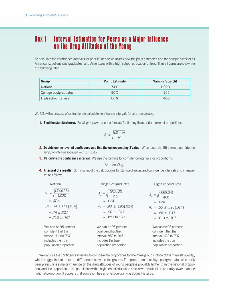
To calculate the confidence intervals for peer influence we must know the point estimates and the sample sizes for all Americans, college postgraduates, and Americans with a high school education or less. These figures are shown in the following table.

Group Point Estimate Sample Size (N)

National 74% 1,020

College postgraduates 90% 155

High school or less 66% 400

We follow the process of estimation to calculate confidence intervals for all three groups.

1. Find the standard error. For all groups we use the formula for finding the standard error of proportions:

Sp p

Np =−( )1

2. Decide on the level of confidence and find the corresponding Z value. We choose the 95 percent confidence level, which is associated with Z = 1.96.

3. Calculate the confidence interval. We use the formula for confidence intervals for proportions:

CI = p ± Z (Sp)

4. Interpret the results. Summaries of the calculations for standard errors and confidence intervals and interpre-tations follow.

National College Postgraduates High School or Less

Sp = . .,

== ± ( )= ±

( )( )

.

( . .

. .

74 261 020

0

0

0

14

CI 74 1.96 14

74 27

= 713 to 767. .

Sp =. .

== ± ( )= ±=

( )( )

.

( . . .

. .

.

90 10155

0

0 0

0 0

24

CI 9 1 96 24

9 47

8853 to 947.

Sp =. .

== ± ( )= ±=

( )( )

.

( . . .

. .

.

66 34400

0

0

0

24

CI 66 1 96 24

66 47

6613 to 7 7. 0

We can be 95 percent confident that the interval .713 to .767 includes the true population proportion.



We can use the confidence intervals to compare the proportions for the three groups. None of the intervals overlap, which suggests that there are differences between the groups. The proportion of college postgraduates who think peer pressure is a major influence on the drug attitudes of young people is probably higher than the national propor-tion, and the proportion of the population with a high school education or less who think this is probably lower than the national proportion. It appears that education has an effect on opinions about this issue.


22 The Process of Statistical Hypothesis Testing

The process of statistical hypothesis testing consists of the following five steps:

1. Making assumptions

2. Stating the research and null hypotheses and selecting alpha

3. Selecting a sampling distribution and a test statistic

4. Computing the test statistic

5. Making a decision and interpreting the results

Examine quantitative research reports, and you will find that all responsible researchers follow these five basic steps, although they may state them less explicitly. When asked to critically review a research report, your criticism should be based on whether the researchers have correctly followed the process of statistical hypothesis testing and if they have used the proper procedures at each step of the process. Others will use the same criteria to evaluate research reports you have written.

In this section we follow the five steps of the process of statistical hypothesis testing. We provide a detailed guide for choosing the appropriate sampling distribution, test statistic, and formulas for the test statistics. In the following sections we will present research examples to show how the process is used in practice.

Step 1: Making Assumptions

Statistical hypothesis testing involves making several assumptions that must be met for the results of the test to be valid. These assumptions include the level of measurement of the variable, the method of sampling, the shape of the population distribution, and the sample size. The specific assumptions may vary, depending on the test or the conditions of testing. However, all statistical tests assume random sampling, and two-sample tests require independent random sampling. Tests of hypotheses about means also assume interval-ratio level of measurement and require that the population under consideration is normally distributed or that the sample size is larger than 50.

Step 2: Stating the Research and Null Hypotheses and Selecting Alpha

Hypotheses are tentative answers to research questions, which can be derived from theory, observations, or intuition. As tentative answers to research questions, hypotheses are generally stated in sentence form. To verify a hypothesis using statistical hypothesis testing, it must be stated in a testable form called a research hypothesis.

We use the symbol H1 to denote the research hypothesis. Hypotheses are always stated in terms of population

parameters. The null hypothesis (H0) is a contradiction of the research hypothesis and is usually a statement of no dif-

ference between the population parameters. It is the null hypothesis that researchers test. If it can be shown that the null hypothesis is false, researchers can claim support for their research hypothesis.

Published research reports rarely make a formal statement of the research and null hypotheses. Researchers gener-ally present their hypotheses in sentence form. In order to evaluate a research report, you must construct the research and null hypotheses to determine whether the researchers actually tested the hypotheses they stated. Box 2 shows pos-sible hypotheses for comparing the sample means and for testing a relationship in a bivariate table.

Statistical hypothesis testing always involves some risk of error because sample data are used to estimate or infer pop-ulation parameters. Two types of error are possible—Type I and Type II. A Type I error occurs when a true null hypothesis is rejected; alpha (α) is the probability of making a Type I error. In social science research alpha is typically set at the .05, .01, or .001 level. At the .05 level, researchers risk a 5 percent chance of making a Type I error. The risk of making a Type I error can be decreased by choosing a smaller alpha level—.01 or .001. However, as the risk of a Type I error decreases, the risk of a Type II error increases. A Type II error occurs when the researcher fails to reject a false null hypothesis.


How does a researcher choose the appropriate alpha level? By weighing the consequences of making a Type I or a Type II error. Let’s look again at research on AIDS. Suppose researchers are testing a new drug that may halt the progression of AIDS. The null hypothesis is that the drug has no effect on the progression of AIDS. Now suppose that preliminary research has shown this drug has serious negative side effects. The researchers would want to minimize the risk of making a Type I error (rejecting a true null hypothesis) so people would not experience the negative side effects unnecessarily if the drug does not affect the progression of AIDS. An alpha level of .001 or smaller would be appropriate.

Alternatively, if preliminary research has shown the drug has no serious negative side effects, the researchers would want to minimize the risk of a Type II error (failing to reject a false null hypothesis). If the null hypothesis is false and the drug might actually help people with AIDS, researchers would want to increase the chance of rejecting the null hypoth-esis. In this case, the appropriate alpha level would be .05.

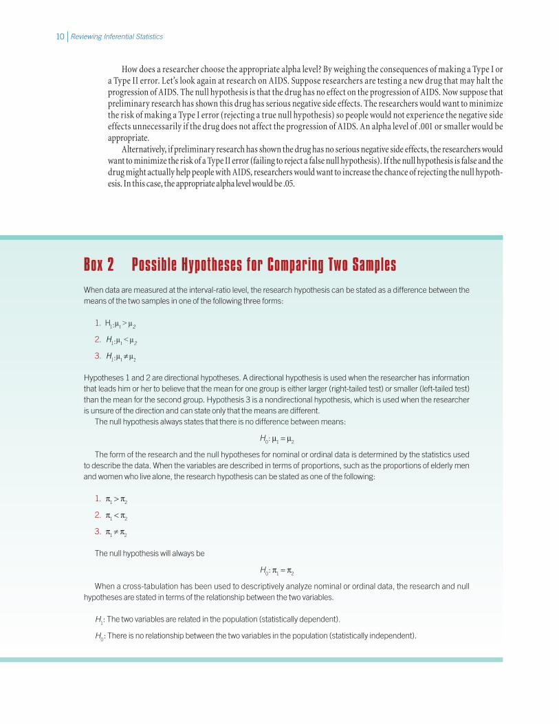
Box 2 Possible Hypotheses for Comparing Two SamplesWhen data are measured at the interval-ratio level, the research hypothesis can be stated as a difference between the means of the two samples in one of the following three forms:

1. 1:µ1 > µ2

2. H1:µ1 < µ2

3. H1:µ1 ≠ µ

2

Hypotheses 1 and 2 are directional hypotheses. A directional hypothesis is used when the researcher has information that leads him or her to believe that the mean for one group is either larger (right-tailed test) or smaller (left-tailed test) than the mean for the second group. Hypothesis 3 is a nondirectional hypothesis, which is used when the researcher is unsure of the direction and can state only that the means are different.

The null hypothesis always states that there is no difference between means:

H0: µ1 = µ2

The form of the research and the null hypotheses for nominal or ordinal data is determined by the statistics used to describe the data. When the variables are described in terms of proportions, such as the proportions of elderly men and women who live alone, the research hypothesis can be stated as one of the following:

1. π1 > π2

2. π1 < π2

3. π1 ≠ π2

The null hypothesis will always be

H0: π1 = π2

When a cross-tabulation has been used to descriptively analyze nominal or ordinal data, the research and null hypotheses are stated in terms of the relationship between the two variables.

H1: The two variables are related in the population (statistically dependent).

H0: There is no relationship between the two variables in the population (statistically independent).


Do not confuse alpha and P. Alpha is the level of probability—determined in advance by the investigator—at which the null hypothesis is rejected; P is the actual calculated probability associated with the obtained value of the test statis-tic. The null hypothesis is rejected when P ≤ alpha.

Step 3: Selecting a Sampling Distribution and a Test Statistic

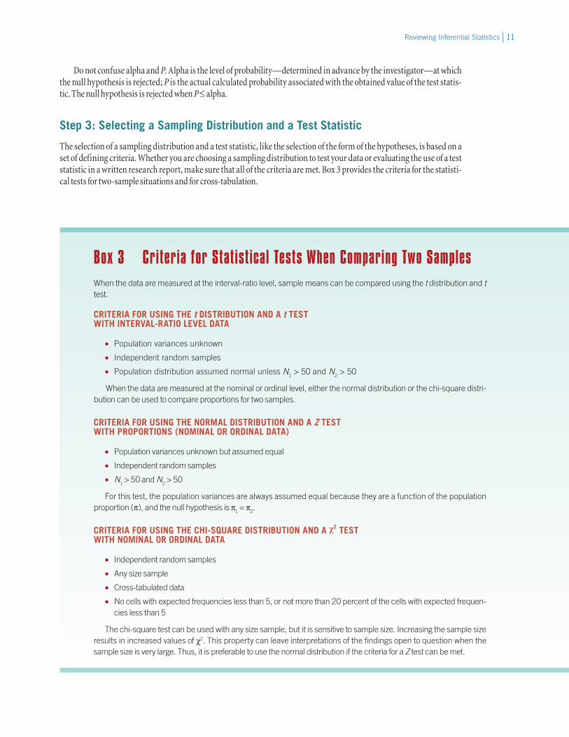
The selection of a sampling distribution and a test statistic, like the selection of the form of the hypotheses, is based on a set of defining criteria. Whether you are choosing a sampling distribution to test your data or evaluating the use of a test statistic in a written research report, make sure that all of the criteria are met. Box 3 provides the criteria for the statisti-cal tests for two-sample situations and for cross-tabulation.

Box 3 Criteria for Statistical Tests When Comparing Two SamplesWhen the data are measured at the interval-ratio level, sample means can be compared using the t distribution and t test.

CRITERIA FOR USING THE t DISTRIBUTION AND A t TEST WITH INTERVAL-RATIO LEVEL DATA

• Population variances unknown

• Independent random samples

• Population distribution assumed normal unless N1 > 50 and N2 > 50

When the data are measured at the nominal or ordinal level, either the normal distribution or the chi-square distri-bution can be used to compare proportions for two samples.

CRITERIA FOR USING THE NORMAL DISTRIBUTION AND A Z TEST WITH PROPORTIONS (NOMINAL OR ORDINAL DATA)

• Population variances unknown but assumed equal


• N1 > 50 and N2 > 50

For this test, the population variances are always assumed equal because they are a function of the population proportion (π), and the null hypothesis is π1 = π2.

CRITERIA FOR USING THE CHI-SQUARE DISTRIBUTION AND A χ2 TEST WITH NOMINAL OR ORDINAL DATA


• Any size sample

• Cross-tabulated data

• No cells with expected frequencies less than 5, or not more than 20 percent of the cells with expected frequen-cies less than 5

The chi-square test can be used with any size sample, but it is sensitive to sample size. Increasing the sample size results in increased values of χ2. This property can leave interpretations of the findings open to question when the sample size is very large. Thus, it is preferable to use the normal distribution if the criteria for a Z test can be met.


Step 4: Computing the Test Statistic

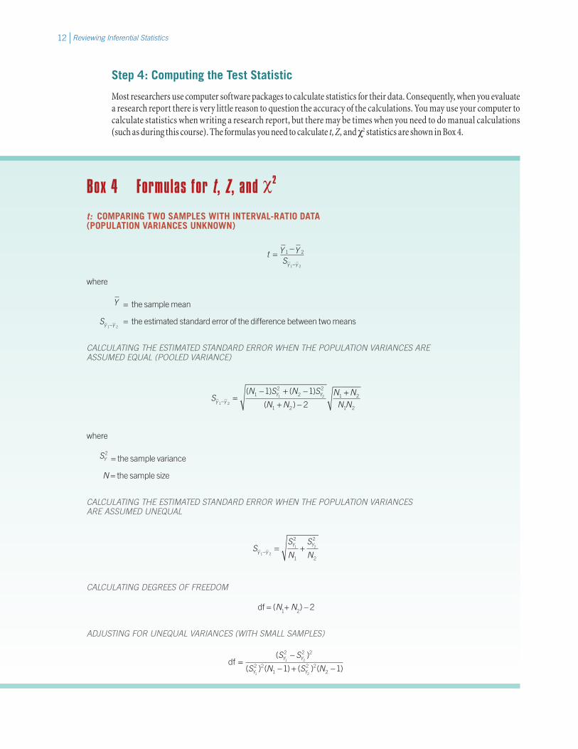
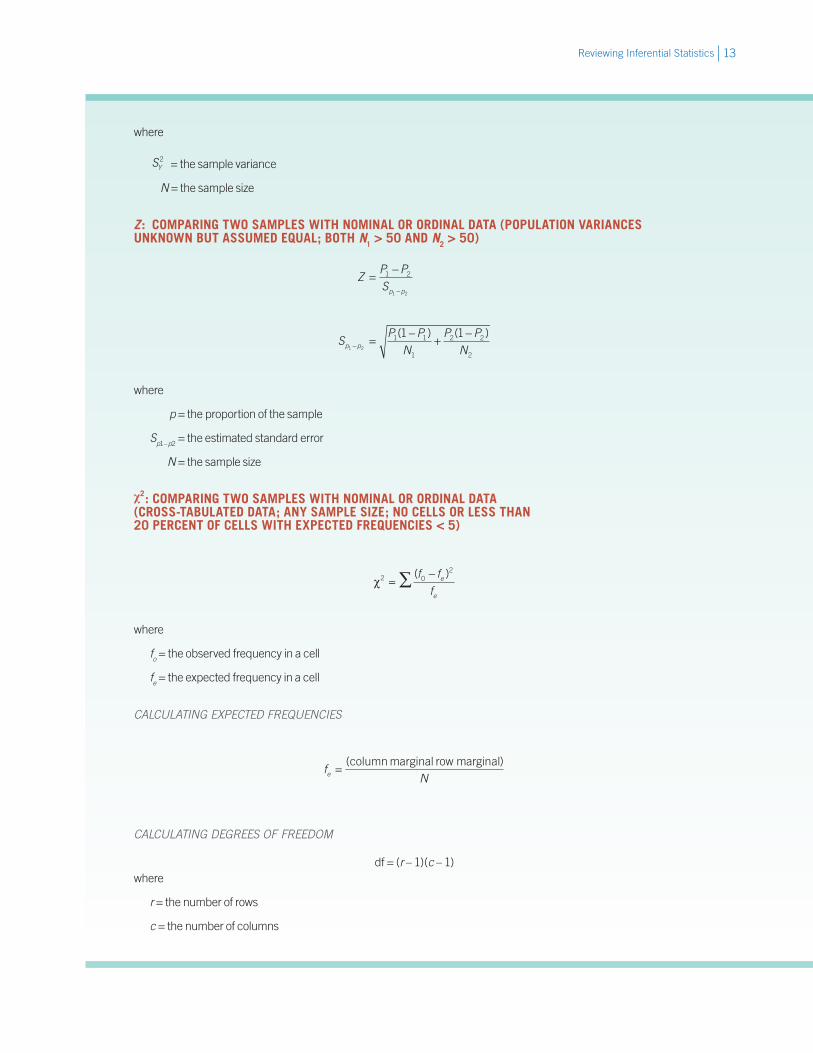
Most researchers use computer software packages to calculate statistics for their data. Consequently, when you evaluate a research report there is very little reason to question the accuracy of the calculations. You may use your computer to calculate statistics when writing a research report, but there may be times when you need to do manual calculations (such as during this course). The formulas you need to calculate t, Z, and χ2 statistics are shown in Box 4.

Box 4 Formulas for t, Z, and χ2

t: COMPARING TWO SAMPLES WITH INTERVAL-RATIO DATA (POPULATION VARIANCES UNKNOWN)

t Y YS

Y Y

=−

−

1 2

1 2

where

Y = the sample mean

SY Y1 2−

= the estimated standard error of the difference between two means

CALCULATING THE ESTIMATED STANDARD ERROR WHEN THE POPULATION VARIANCES ARE ASSUMED EQUAL (POOLED VARIANCE)

SN S N S

N NN NN NY Y

Y Y

1 2

1 212

22

1 2

1 2

1 2

1 1

2− =− + −

+ −+( ) ( )

( )

where

SY2 = the sample variance

N = the sample size

CALCULATING THE ESTIMATED STANDARD ERROR WHEN THE POPULATION VARIANCES ARE ASSUMED UNEQUAL

SS

N

S

NY Y

Y Y

1 2

1 2

2

1

2

2− = +

CALCULATING DEGREES OF FREEDOM

df = (N1+ N2) – 2

ADJUSTING FOR UNEQUAL VARIANCES (WITH SMALL SAMPLES)

df =−

− + −( )

( ) ( ) ( ) ( )

S S

S N S NY Y

Y Y

1 2

1 2

2 2 2

2 21

2 221 1


where

SY2 = the sample variance

N = the sample size

Z : COMPARING TWO SAMPLES WITH NOMINAL OR ORDINAL DATA (POPULATION VARIANCES UNKNOWN BUT ASSUMED EQUAL; BOTH N1 > 50 AND N2 > 50)

ZP PSp p

=−

−

1 2

1 2

SP P

NP P

Np p1 2

1 1

1

2 2

2

1 1− =

−+

−( ) ( )

where

p = the proportion of the sample

Sp1 – p2 = the estimated standard error

N = the sample size

χ2: COMPARING TWO SAMPLES WITH NOMINAL OR ORDINAL DATA (CROSS-TABULATED DATA; ANY SAMPLE SIZE; NO CELLS OR LESS THAN 20 PERCENT OF CELLS WITH EXPECTED FREQUENCIES < 5)

χ2 02

=−∑ ( )f ff

e

e

where

fo = the observed frequency in a cell

fe = the expected frequency in a cell

CALCULATING EXPECTED FREQUENCIES

fNe =

( )column marginal row marginal

CALCULATING DEGREES OF FREEDOM

df = (r – 1)(c – 1)where

r = the number of rows

c = the number of columns


Step 5: Making a Decision and Interpreting the Results

The last step in the formal process of statistical hypothesis testing is to determine whether the null hypothesis should be rejected. If the probability of the obtained statistic—t, Z, or χ2—is equal to or less than alpha, it is considered to be statistically significant and the null hypothesis is rejected. If the null hypothesis is rejected, the researcher can claim support for the research hypothesis. In other words, the hypothesized answer to the research question becomes less tentative, but the researcher cannot state that it is absolutely true because there is always some error involved when samples are used to infer population parameters.

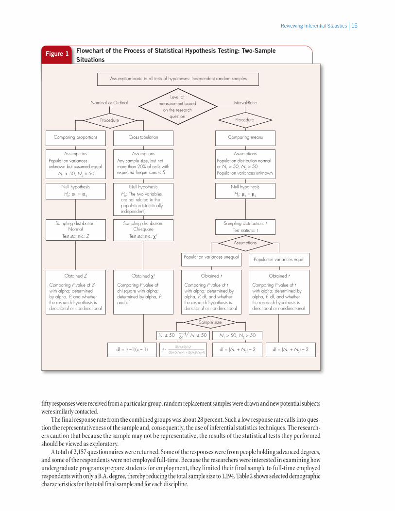
The conditions and assumptions associated with the two-sample tests are summarized in the flowchart presented in Figure 1. Use this f lowchart to help you decide which of the different tests (t, Z, or chi-square) is appropriate under what conditions and how to choose the correct formula for calculating the obtained value for the test.

22 Statistics in Practice: Education and Employment

Why did you decide to attend college? Whether you made the decision on your own or discussed it with your parents, spouse, or friends, the prospect of increased employment opportunities and higher income after graduation probably weighed heavily in your decision. Although most college students expect that their major will prepare them to compete successfully in the job market and the workplace, undergraduate programs do not always meet this expectation.

In their introduction to a 1992 study of the efficacy of social science undergraduate programs, Velasco, Stockdale, and Scrams3 note that sociology programs have traditionally been designed to prepare students for graduate school, where they can earn professional status. However, the vast majority of students who earn a B.A. in sociology do not attend graduate school and must either earn their professional status through work experience or find employment in some other sector. The result is that many people holding a B.A. in sociology are underemployed.

According to Velasco et al., certain foundational skills are critical to successful careers in the social sciences. These foundational skills include logical reasoning, understanding scientific principles, mathematical and statistical skills, computer skills, and knowing the subject matter of the major. In their study, the researchers sought to determine how well sociology programs develop these skills in students. Specifically, they focused on the following research questions.

1. How do sociology alumni with B.A. degrees, as compared with other social science alumni, rate their major with respect to the helpfulness of their major in developing the “foundational skills”?

2. Has the percentage of sociology alumni who rate their major highly increased over time with respect to the devel-opment of these skills?

3. Do male and female alumni from the five social science disciplines differ in regard to ratings of the major in developing the foundational skills? Do male and female alumni differ with respect to occupational prestige or personal income?4

Clearly, surveying the entire population of alumni in five disciplines to obtain answers to these questions would be a nearly insurmountable task. To make their project manageable, the researchers surveyed a sample of each population and used inferential statistics to analyze the data. Their sampling technique and characteristics of the samples are dis-cussed in the next section.

Sampling Technique and Sample Characteristics

Velasco et al. used the alumni records from eight diverse campuses in the California State University system to identify graduates of B.A. programs in anthropology, economics, political science, psychology, and sociology. The population con-sisted of forty groups of alumni (5 disciplines × 8 campuses = 40 groups). The researchers drew a random sample from each group.5 Potential subjects were sent a questionnaire and, if necessary, a follow-up postcard. If after follow-up fewer than

3Steven C. Velasco, Susan E. Stockdale, and David J. Scrams, “Sociology and Other Social Sciences: California State University Alumni Ratings of the B.A. Degree for Development of Employment Skills,” Teaching Sociology 20 (1992): 60–70.

4Ibid., p. 62.

5All members of groups with fewer than 150 members were included as potential sub jects. Up to three questionnaire and follow-up mailings were made to each alumnus to maximize responses from these groups.


Figure 1 Flowchart of the Process of Statistical Hypothesis Testing: Two-Sample Situations

Sampling distribution: tTest statistic: t

Assumption basic to all tests of hypotheses: Independent random samples

Obtained t

Level ofmeasurement based

on the researchquestion

Interval-RatioNominal or Ordinal

Procedure

AssumptionsPopulation variances unknown but assumed equal

N1 > 50, N2 > 50

AssumptionsAny sample size, but not more than 20% of cells with expected frequencies < 5

AssumptionsPopulation distribution normal or N1 > 50, N2 > 50 Population variances unknown

Null hypothesisH0: The two variables are not related in the population (statistically independent).

Null hypothesisH0: µ1 = µ2

Obtained χ2 Obtained tObtained Z

Comparing meansCross-tabulationComparing proportions

Null hypothesisH0: π1 = π2

Sampling distribution: Normal

Test statistic: Z

Sampling distribution: Chi-square

Test statistic: χ2

Assumptions

Population variances unequal Population variances equal

Comparing P value of Z with alpha; determined by alpha, P, and whether the research hypothesis is directional or nondirectional

Comparing P value of chi-square with alpha; determined by alpha, P, and df

Comparing P value of t with alpha; determined by alpha, P, df, and whether the research hypothesis is directional or nondirectional

Comparing P value of t with alpha; determined by alpha, P, df, and whether the research hypothesis is directional or nondirectional

Sample size

N1 > 50; N2 > 50

df = (S2

1/n1+S22/n2)

2

(S21/n1)

2/(n1–1) + (S22/n2)

2/(n2–1)df = (r –1)(c – 1) df = (N1 + N2) – 2df = (N1 + N2) – 2

N1 ≤ 50 or N1 ≤ 50and/

Procedure

fifty responses were received from a particular group, random replacement samples were drawn and new potential subjects were similarly contacted.

The final response rate from the combined groups was about 28 percent. Such a low response rate calls into ques-tion the representativeness of the sample and, consequently, the use of inferential statistics techniques. The research-ers caution that because the sample may not be representative, the results of the statistical tests they performed should be viewed as exploratory.

A total of 2,157 questionnaires were returned. Some of the responses were from people holding advanced degrees, and some of the respondents were not employed full-time. Because the researchers were interested in examining how undergraduate programs prepare students for employment, they limited their final sample to full-time employed respondents with only a B.A. degree, thereby reducing the total sample size to 1,194. Table 2 shows selected demographic characteristics for the total final sample and for each discipline.


Comparing Ratings of the Major Between Sociology and Other Social Science Alumni

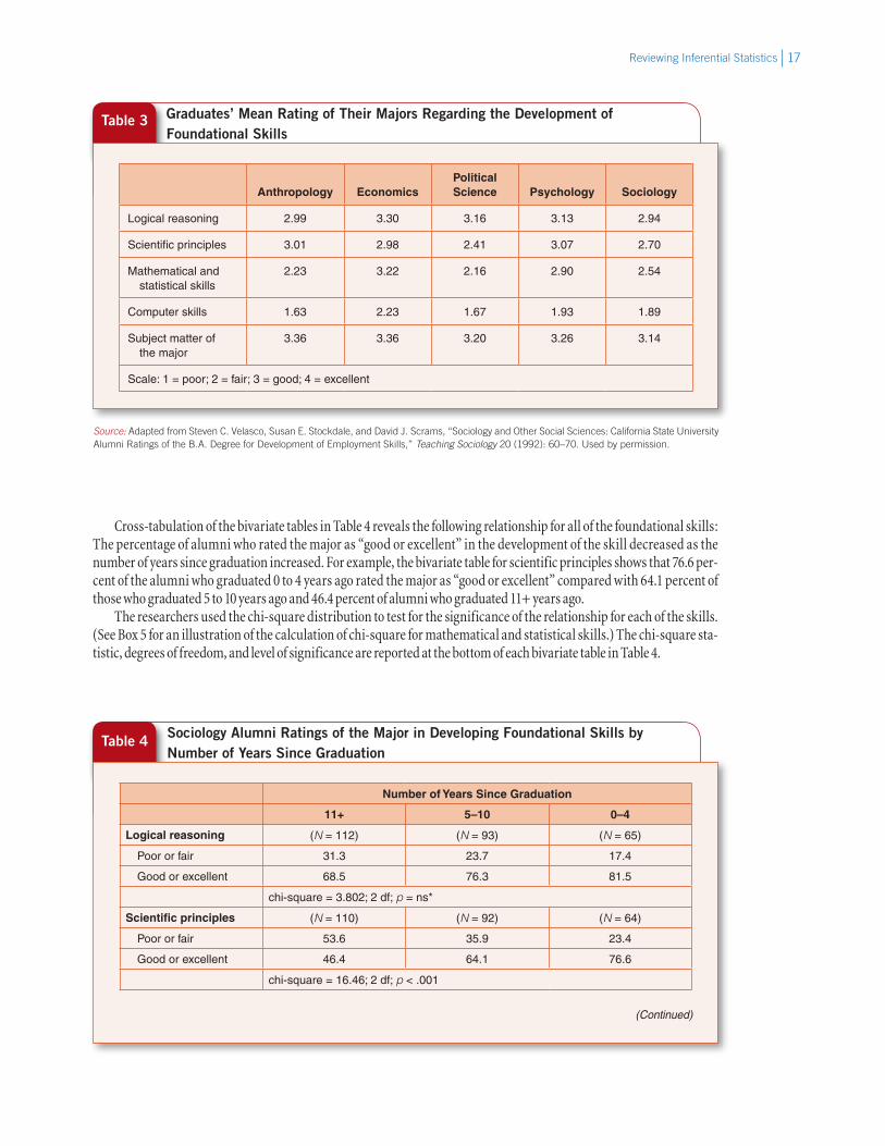
The first research question in this study required a comparison between sociology alumni ratings of their major on the development of foundational skills and the ratings given by alumni from other social science disciplines. To gather data on foundational skills, the researchers asked alumni to rate how well their major added to the development of each of the five skills, using the following scale: 1 = poor; 2 = fair; 3 = good; 4 = excellent. The mean rating for each of the founda-tional skills, by major, is shown in Table 3. The table shows that the skill rated most highly in all disciplines was subject matter of the major. Looking at the mean ratings, we can determine that economics alumni generally rated their major the highest, whereas sociology and political science alumni rated their majors the lowest overall.6 The lowest rating in all disciplines was given to the development of computer skills.

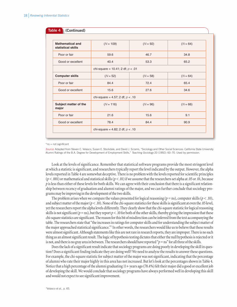
Ratings of Foundational Skills in Sociology: Changes over Time

In recent years many sociology departments have taken steps to align undergraduate requirements more closely with the qualifications necessary for a career in sociology. If these changes have been successful, then more recent graduates should rate program development of foundational skills higher than less recent graduates. This is the second research question addressed in this study. To examine the question of whether the percentage of so ciology alumni who rate their major highly with respect to the development of foundational skills has increased over time, Velasco et al. grouped the sample of sociology alumni into three categories by number of years since graduation: 11+ years, 5–10 years, and 0–4 years. They grouped the ratings into two categories: “poor or fair” and “good or excellent.” Table 4 shows percentage bivariate tables for each of the five foundation skills.

Table 2 Selected Demographic Characteristics of the Sample Population with Bachelor’s Degrees Who Are Employed Full-Time

All Anthropology EconomicsPolitical Science Psychology Sociology

N 1,194 181 288 222 220 283

% sample in major

— 15.2 24.1 18.6 18.4 23.7

% female 48.7 64.1 26.4 31.5 66.4 61.1

% white 84.8 87.3 87.2 83.3 86.4 80.6

Mean age 35.5 37.6 34.7 33.4 34.1 37.9

SD age 9.1 10.1 9.3 8.2 8.5 8.8

Mean graduation age

27.2 29.9 26.0 25.5 26.6 28.3

SD graduation age

7.8 9.9 6.8 6.4 7.0 8.0

Source: Steven C. Velasco, Susan E. Stockdale, and David J. Scrams, “Sociology and Other Social Sciences: California State University Alumni Ratings of the B.A. Degree for Development of Employment Skills,” Teaching Sociology 20 (1992): 60–70. Used by permission.

6In this text we limit our discussion to tests of differences between two sample means. Procedures for comparing more than two mean scores are reviewed in our Web chapter “Analysis of Variance.” Velasco et al. used analysis of variance (ANOVA) to test for differ-ences among five disciplines and found that there were significant differences in the ratings given each foundational skill across majors.


Cross-tabulation of the bivariate tables in Table 4 reveals the following relationship for all of the foundational skills: The percentage of alumni who rated the major as “good or excellent” in the development of the skill decreased as the number of years since graduation increased. For example, the bivariate table for scientific principles shows that 76.6 per-cent of the alumni who graduated 0 to 4 years ago rated the major as “good or excellent” compared with 64.1 percent of those who graduated 5 to 10 years ago and 46.4 percent of alumni who graduated 11+ years ago.

The researchers used the chi-square distribution to test for the significance of the relationship for each of the skills. (See Box 5 for an illustration of the calculation of chi-square for mathematical and statistical skills.) The chi-square sta-tistic, degrees of freedom, and level of significance are reported at the bottom of each bivariate table in Table 4.

Table 3 Graduates’ Mean Rating of Their Majors Regarding the Development of Foundational Skills

Anthropology EconomicsPolitical Science Psychology Sociology

Logical reasoning 2.99 3.30 3.16 3.13 2.94

Scientific principles 3.01 2.98 2.41 3.07 2.70

Mathematical and statistical skills

2.23 3.22 2.16 2.90 2.54

Computer skills 1.63 2.23 1.67 1.93 1.89

Subject matter of the major

3.36 3.36 3.20 3.26 3.14

Scale: 1 = poor; 2 = fair; 3 = good; 4 = excellent

Source: Adapted from Steven C. Velasco, Susan E. Stockdale, and David J. Scrams, “Sociology and Other Social Sciences: California State University Alumni Ratings of the B.A. Degree for Development of Employment Skills,” Teaching Sociology 20 (1992): 60–70. Used by permission.

Table 4 Sociology Alumni Ratings of the Major in Developing Foundational Skills by Number of Years Since Graduation

Number of Years Since Graduation

11+ 5–10 0–4

Logical reasoning (N = 112) (N = 93) (N = 65)

Poor or fair 31.3 23.7 17.4

Good or excellent 68.5 76.3 81.5

chi-square = 3.802; 2 df; p = ns*

Scientific principles (N = 110) (N = 92) (N = 64)

Poor or fair 53.6 35.9 23.4


chi-square = 16.46; 2 df; p < .001

(Continued)


Look at the levels of significance. Remember that statistical software programs provide the most stringent level at which a statistic is significant, and researchers typically report the level indicated by the output. However, the alpha levels reported in Table 4 are somewhat deceptive. There is no problem with the levels reported for scientific principles (p < .001) or mathematical and statistical skills (p < .01) if we assume that the researchers set alpha at .05 or .01, because p is less than either of these levels for both skills. We can agree with their conclusion that there is a significant relation-ship between recency of graduation and alumni ratings of the major, and we can further conclude that sociology pro-grams may be improving in the development of the two skills.

The problem arises when we compare the values presented for logical reasoning (p = ns), computer skills (p < .10), and subject matter of the major (p < .10). None of the chi-square statistics for these skills is significant at even the .05 level, yet the researchers report the alpha levels differently. They clearly show that the chi-square statistic for logical reasoning skills is not significant (p = ns), but they report p < .10 for both of the other skills, thereby giving the impression that these chi-square statistics are significant. The reason for this bit of misdirection can be inferred from the text accompanying the table. The researchers state that “the increases in ratings for computer skills and for understanding the subject matter of the major approached statistical significance.”7 In other words, the researchers would like us to believe that these results were almost significant. Although statements like this are not rare in research reports, they are improper. There is no such thing as an almost significant result. The logic of hypothesis testing dictates that either the null hypothesis is rejected or it is not, and there is no gray area in between. The researchers should have reported “p = ns” for all three of the skills.

Does the lack of a significant result indicate that sociology programs are doing poorly in developing the skill in ques-tion? Does a significant finding indicate they are doing well? We need to analyze the results to answer these questions. For example, the chi-square statistic for subject matter of the major was not significant, indicating that the percentage of alumni who rate their major highly in this area has not increased. But let’s look at the percentages shown in Table 4. Notice that a high percentage of the alumni graduating 11+ years ago (78.4%) felt their major did a good or excellent job of developing the skill. We would conclude that sociology programs have always performed well in developing this skill and would not expect to see significant improvement.

Table 4 (Continued)

Mathematical and statistical skills

(N = 109) (N = 92) (N = 64)

Poor or fair 59.6 46.7 34.8


chi-square = 10.41; 2 df; p < .01

Computer skills (N = 52) (N = 58) (N = 64)

Poor or fair 84.4 72.4 65.4


chi-square = 4.57; 2 df; p < .10

Subject matter of the major

(N = 116) (N = 96) (N = 66)

Poor or fair 21.6 15.6 9.1


chi-square = 4.82; 2 df; p < .10

*ns = not significant


7Velasco et al., p. 65.


Gender Differences in Ratings of Foundational Skills, Occupational Prestige, and Income

The final research question explored by Velasco et al. concerned gender differences in alumni ratings of foundational skills, occupational prestige, and income. A foundational skills index was constructed by summing the responses for the five categories of skills for each alumnus. The index ranged from 5 to 20, and the mean index score was calculated for each of the disciplines by gender. Occupational prestige was coded using a recognized scale and job titles provided by respondents. Information on income was gathered by asking respondents to report their approximate annual income.

Learning Check. Analyze the results for the remaining four skills. Where is improvement necessary? Where is it less critical?

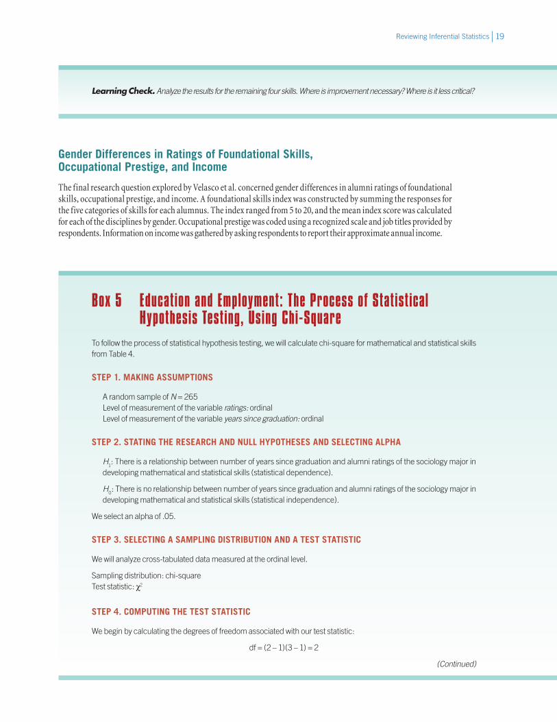
Box 5 Education and Employment: The Process of Statistical Hypothesis Testing, Using Chi-Square

To follow the process of statistical hypothesis testing, we will calculate chi-square for mathematical and statistical skills from Table 4.

STEP 1. MAKING ASSUMPTIONS

A random sample of N = 265Level of measurement of the variable ratings: ordinalLevel of measurement of the variable years since graduation: ordinal

STEP 2. STATING THE RESEARCH AND NULL HYPOTHESES AND SELECTING ALPHA

H1: There is a relationship between number of years since graduation and alumni ratings of the sociology major in developing mathematical and statistical skills (statistical dependence).

H0: There is no relationship between number of years since graduation and alumni ratings of the sociology major in developing mathematical and statistical skills (statistical independence).

We select an alpha of .05.

STEP 3. SELECTING A SAMPLING DISTRIBUTION AND A TEST STATISTIC

We will analyze cross-tabulated data measured at the ordinal level.

Sampling distribution: chi-squareTest statistic: χ2

STEP 4. COMPUTING THE TEST STATISTIC

We begin by calculating the degrees of freedom associated with our test statistic:

df = (2 – 1)(3 – 1) = 2

(Continued)


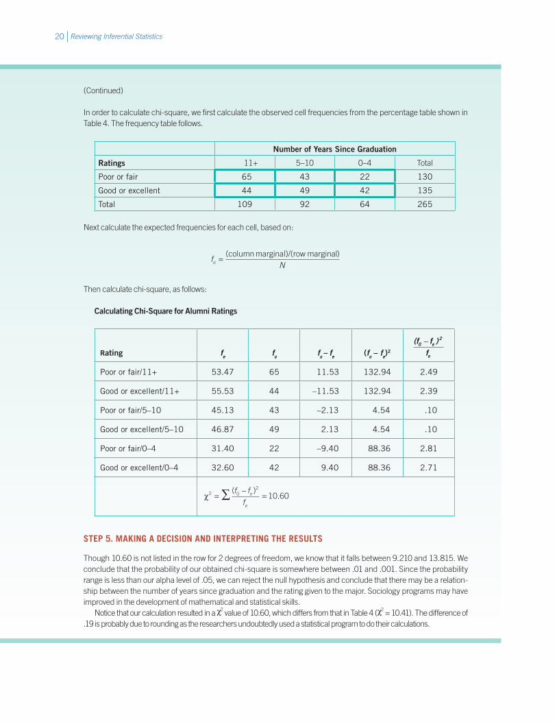
(Continued)

In order to calculate chi-square, we first calculate the observed cell frequencies from the percentage table shown in Table 4. The frequency table follows.

Number of Years Since Graduation

Ratings 11+ 5–10 0–4 Total

Poor or fair 65 43 22 130

Good or excellent 44 49 42 135

Total 109 92 64 265

Next calculate the expected frequencies for each cell, based on:

fNe = ( )column marginal)/(row marginal

Then calculate chi-square, as follows:

Calculating Chi-Square for Alumni Ratings

Rating fe fo fo – fe (fo – fe)2

(f f )f

0 e2

e

−

Poor or fair/11+ 53.47 65 11.53 132.94 2.49

Good or excellent/11+ 55.53 44 –11.53 132.94 2.39

Poor or fair/5–10 45.13 43 –2.13 4.54 .10

Good or excellent/5–10 46.87 49 2.13 4.54 .10

Poor or fair/0–4 31.40 22 –9.40 88.36 2.81

Good or excellent/0–4 32.60 42 9.40 88.36 2.71

χ2 02

10 60=−

=∑ ( ).

f ff

e

e

STEP 5. MAKING A DECISION AND INTERPRETING THE RESULTS

Though 10.60 is not listed in the row for 2 degrees of freedom, we know that it falls between 9.210 and 13.815. We conclude that the probability of our obtained chi-square is somewhere between .01 and .001. Since the probability range is less than our alpha level of .05, we can reject the null hypothesis and conclude that there may be a relation-ship between the number of years since graduation and the rating given to the major. Sociology programs may have improved in the development of mathematical and statistical skills.

Notice that our calculation resulted in a χ2 value of 10.60, which differs from that in Table 4 (χ2 = 10.41). The difference of .19 is probably due to rounding as the researchers undoubtedly used a statistical program to do their calculations.


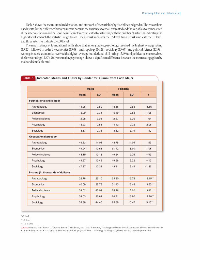
Table 5 shows the mean, standard deviation, and t for each of the variables by discipline and gender. The researchers used t tests for the difference between means because the variances were all estimated and the variables were measured at the interval-ratio or ordinal level. Significant t’s are indicated by asterisks, with the number of asterisks indicating the highest level at which the statistic is significant. One asterisk indicates the .05 level, two asterisks indicate the .01 level, and three asterisks indicate the .001 level.

The mean ratings of foundational skills show that among males, psychology received the highest average rating (15.23), followed in order by economics (15.09), anthropology (14.28), sociology (13.67), and political science (12.98). Among females, economics received the highest average foundational skill rating (15.49) and political science received the lowest rating (12.67). Only one major, psychology, shows a significant difference between the mean ratings given by male and female alumni.

Table 5 Indicated Means and t Tests by Gender for Alumni from Each Major

Males Females

Mean SD Mean SD t

Foundational skills index

Anthropology 14.28 2.80 13.58 2.83 1.56

Economics 15.09 2.74 15.49 2.83 –1.08

Political science 12.98 3.08 12.67 3.36 .64

Psychology 15.23 2.84 14.42 2.22 2.06*

Sociology 13.67 2.74 13.52 3.19 .40

Occupational prestige

Anthropology 49.83 14.01 48.75 11.04 .53

Economics 49.94 10.53 51.42 8.90 –1.08

Political science 48.19 10.18 49.54 9.05 –.93

Psychology 49.37 10.43 49.56 9.22 –.13

Sociology 47.27 10.32 48.81 9.45 –1.25

Income (in thousands of dollars)

Anthropology 32.78 22.10 23.30 13.78 3.15**

Economics 40.09 22.73 31.43 15.44 3.53***

Political science 38.52 43.01 25.96 8.60 3.42***

Psychology 34.03 26.61 24.71 13.90 2.70**

Sociology 39.36 44.40 25.66 10.47 3.13**

*p < .05

**p < .01

***p < .001



The mean occupational prestige scores are similar across disciplines within genders. They are also similar across genders within disciplines. The results of the t tests show no significant differences between the mean occupational pres-tige scores for male and female alumni from any major. In Box 6 we use the process of statistical hypothesis testing to calculate t for occupational prestige among sociology alumni.

Box 6 Occupational Prestige of Male and Female Sociology Alumni: Another Example Using a t TestThe means, standard deviations, and sample sizes necessary to calculate t for occupational prestige as shown in Table 5 are shown below.

Mean SD N

Males 47.27 10.32 105

Females 48.81 1 9.45 162

STEP 1. MAKING ASSUMPTIONS

Independent random samples

Level of measurement of the variable occupational prestige: interval-ratio

Population variances unknown but assumed equal

Because N1 > 50 and N2 > 50, the assumption of normal population is not required.

STEP 2. STATING THE RESEARCH AND NULL HYPOTHESES AND SELECTING ALPHA

Our hypothesis will be nondirectional because we have no basis for assuming the occupational prestige of one group is higher than the occupational prestige of the other group:

H1: µ1 ≠ µ2

H0: µ1 = µ2

Alpha for our test will be .05.

STEP 3. SELECTING A SAMPLING DISTRIBUTION AND A TEST STATISTIC

We will analyze data measured at the interval-ratio level with estimated variances assumed equal.

Sampling distribution: t distributionTest statistic: t

STEP 4. COMPUTING THE TEST STATISTIC

Degrees of freedom aredf = (N1 + N2) – 2 = (105 + 162) – 2 = 265


Economics majors have the highest mean annual income for both males ($40,090) and females ($31,430); anthro-pology majors have the lowest mean incomes (males, $32,780; females, $23,300). The results of the t tests (for directional tests) show that the mean income of male alumni is significantly higher than the mean income of female alumni for each major. This finding is not surprising; we know that women typically earn less than men. It is interesting, however, that no significant differences were found between the mean ratings of occupational prestige of male and female alumni. This may indicate that females are paid less than males for similar work.

SPSS Demonstration

The formulas we need to calculate t are

t Y YS

Y Y

=−

−

1 2

1 2

SN S N S

N NN NN NY Y1 2

1 12

2 22

1 2

1 2

1 2

1 12− =

− + −+ −

+( ) ( )( )

First calculate the standard deviation of the sampling distribution:

SY Y1 2

104 10 32 161 9 45105 162 2

105 162105 1

2 2

− =. + .

+ −+( )( ) ( )( )

( ) ( )( 662

11 076 25 14 377 70265

26717 010

9 801 1 125 1 23

)

( )

=, . + , .

,= . . = .

Then plug this figure into the formula for t :

t =. − .

.=

− ..

= − .47 27 48 81

1 231 54

1 231 25

STEP 5. MAKING A DECISION AND INTERPRETING THE RESULTS

Our obtained t is –1.25, indicating that the difference should be evaluated at the left-tail of the t distribution. Based on a two-tailed test, with 265 degrees of freedom, we can determine the probability of –1.25. Recall that we will ignore the negative sign when assessing its probability. Our obtained t is less than any of the listed t values in the last row. The probability of 1.25 is greater than .20, larger than our alpha of .05. We fail to reject the null hypothesis and conclude that there is no difference in occupational prestige between male and female sociology alumni.

Regression Revisited: An Application of Inferential Statistics [Module GSS98PFP-B]

Regression is defined as a measure of association between interval (or ordinal) variables. In this demonstration we review regression mod-els, this time introducing their relationship to statistical hypothesis testing.

As we’ve demonstrated with t, Z, and χ2 statistics, each is part of a statistical hypothesis test procedure. In determining whether our findings are rare or unexpected, we are testing whether our obtained statistic could be based on chance or if something significant is indi-cated between the variables that we’re investigating.

This same logic can be applied to the correlation coefficient, r, and the standardized slope, b. The appropriate distribution to assess the significance of r and b is the t distribution. In every SPSS Correlation


output, SPSS automatically calculates the probability of r based on a two-tailed test. In each regression model, SPSS reports the corresponding t (obtained) and the probability of t for b.

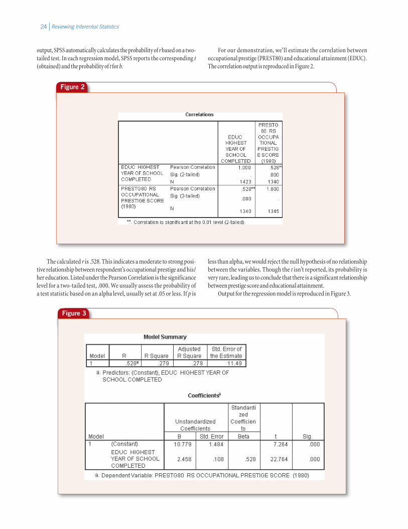
For our demonstration, we’ll estimate the correlation between occupational prestige (PREST80) and educational attainment (EDUC). The correlation output is reproduced in Figure 2.

Figure 2

The calculated r is .528. This indicates a moderate to strong posi-tive relationship between respondent’s occupational prestige and his/her education. Listed under the Pearson Correlation is the significance level for a two-tailed test, .000. We usually assess the probability of a test statistic based on an alpha level, usually set at .05 or less. If p is

less than alpha, we would reject the null hypothesis of no relationship between the variables. Though the t isn’t reported, its probability is very rare, leading us to conclude that there is a significant relationship between prestige score and educational attainment.

Output for the regression model is reproduced in Figure 3.

Figure 3


In the Model Summary table, the correlation coefficient is reported. We know from the previous correlation output that .528 is significant at the .000 level. Let’s consider the data in the Coefficients table.

We will not interpret the significance of the constant (a), but will analyze the information for EDUC. Both the unstandardized and standardized coefficients (Beta) for EDUC are reported. As

indicated by b, for every additional year of education, occupa-tional prestige is predicted to increase by 2.458 units. In the last two columns of the table, the t statistic and its significance level (or p value) are reported for the constant (a) and EDUC. Note that the t statistic for the EDUC coefficient is 22.764, significant at .000. Educational attainment has a very significant positive relationship with occupational prestige.

SPSS Problems

1. Two questions in the GSS98PFP-B file are concerned with respon-dent’s confidence in the federal government (CONFED) and con-fidence in the military (CONARMY). Investigate the relationship between these questions and education (DEGREE). Identify the level of measurement for each variable. Calculate an appropriate statisti-cal test, and describe the relationships you find. Also, describe any differences in the relationships between education and these two confidence variables.

2. Test the null hypothesis that there is no difference in years of edu-cation between those who attended religious services at least one month and those who did not (ATTEND). Use the variable EDUC as the measure of educational attainment in years. Conduct your test at the .05 alpha level. Use data module GSS98PFP-A.

3. What is the relationship between educational attainment (EDUC) and respon dent’s age (AGE) as independent variables and hours of television viewing per week? Confirm how each of these variables is measured and scaled before beginning the exercise.

a. Construct scatterplots to relate TVHOURS to EDUC and AGE. (You should have two scatterplots.) Do the relationships appear to be linear? Describe the relationships.

b. Calculate the correlation coefficient for each scatterplot, and the co efficient of determination. Describe the relationship between the variables.

c. Calculate the regression equation for each scatterplot. Describe the relationship between the variables.

d. Repeat a–c, this time computing separate scatterplots and statistics for men and women (SEX). What can you conclude?

4. Based on the GSS98PFP module:

a. Test at the .01 level the null hypothesis that there is no difference between the proportion of men and women who believe that the elderly should live with their children. In order to answer this question, you’ll have to use the variables SEX and AGED. Use SPSS to determine the percentage of men and the percentage of women who responded to the AGED category “good idea.” (Make note of the total number of each sample.) Then calculate the appropriate two-sample test. You’ll have to do this by hand. What did you find?

b. Is there a difference in educational attainment between whites and blacks in the GSS98 sample? Use SPSS to calculate the appropriate two-sample test (set alpha at .05). Make sure to use the variables RACE [(selecting cases equal to 1 (White) or 2 (Black)] and EDUC. What can you conclude?

Chapter Exercises

1. The 1987–1988 National Survey of Families and Households found, in a sample of 6,645 married couples, that the average length of time a marriage had lasted was 205 months (about 17 years), with a standard deviation of 181 months. Assume that the distribution of marriage length is approximately normal.

a. What proportion of marriages lasts between 10 and 20 years?

b. A marriage that lasts 50 years is commonly viewed as exceptional. What is the percentile rank of a marriage that lasts 50 years? Do you believe this justifies the idea that such a marriage is exceptional?

c. What is the probability that a marriage will last more than 30 years?

d. Is there statistical evidence (from the data in this exercise) to lead you to question the assumption that length of marriage is normally distributed?

2. The 1998 National Election Study included a question on whether individuals approved of President Clinton’s handling of the economy. Responses to this question are most likely related to many demo-graphic and other attitudinal measures. The following table shows the relationship between this item and the respondent’s political preference (five categories).


a. Describe the relationship in this table by calculating appropriate percentages.

b. Test at the .01 alpha level whether political preference and approval of Clinton’s handling of the economy are unrelated.

c. Are all the assumptions for doing a chi-square test met?

3. To investigate Exercise 2 further, the previous table is broken into the following two subtables for those with a high school education or less and those with some college or a college degree. Individuals who did not report their educational level are not included in the table. Use them to answer these questions.

Support for Clinton’s Handling of the Economy

Republican IndependentNo

PreferenceOther Party Democrat Total

Approve strongly 100 145 46 5 377 673

Approve 127 116 30 5 74 352

Disapprove 47 21 9 3 10 90

Disapprove strongly 51 40 4 3 10 108

Total 325 322 89 16 471 1223

Support for Clinton’s Handling of the Economy: Less Than High School or High School Graduate




Approve 32 51 12 0 36 131

Disapprove 16 9 5 0 6 36


Total 107 139 46 1 226 519

Support for Clinton’s Handling of the Economy: Some College or More




Approve 94 65 17 5 36 217

Disapprove 31 12 4 3 4 54


Total 216 183 41 15 241 696

3. (continued)

a. Test at the .05 alpha level the relationship between political preference and support for former President Clinton’s handling of the economy in each table. Are the results consistent or different by educational level?

b. Is educational attainment an intervening variable, or is it acting to specify the relationship between political preference and attitude toward Clinton’s handling of the American economy?

c. If the assumptions of calculating chi-square are not met in these tables, how might you group the categories of political preference


to do a satisfactory test? Do this, and recalculate chi-square for both tables. What do you find now?

d. Can you suggest substantive reasons for the differences between those with a high school education or less and those with at least some college education?

4. A large labor union is planning a survey of its members to ask their opin-ion on several important issues. The members work in large, medium, and small firms. Assume that there are 50,000 members in large compa-nies, 35,000 in medium-sized firms, and 5,000 in small firms.

a. If the labor union takes a proportionate stratified sample of its members of size 1,000, how many union members will be chosen from medium-sized firms?

b. If one member is selected at random from the population, what is the probability that she will be from a small firm?

c. The union decides to take a disproportionate stratified sample with equal numbers of members from each size of firm (to make sure a sufficient number of members from small firms are included). If a sample size of 900 is used, how many members from small firms will be in the sample?

5. The U.S. Census Bureau reported that in 1998, 69 percent of all Hispanic households were two-parent households. You are studying a large city in the Southwest and have taken a random sample of the households in the city for your study. You find that only 59.5 percent of all Hispanic households had two parents in your sample of 400.

a. What is the 95 percent confidence interval for your population estimate of 59.5 percent?

b. What is the 99 percent confidence interval for your population estimate of 59.5 percent?

6. It is often said that there is a relationship between religious belief and education, with belief declining as education increases. However, the recent revival of fundamentalism may have weakened this relationship. The 1998 National Election Study data can be used to investigate this question. One item asked whether religion was important to the respondent, with possible responses of either “Yes” or “No.” We find that those who answered yes have 13.28 mean years of education, with a standard deviation of 2.58; those who answered no have 13.85 mean years of education, with a standard deviation of 2.48. A total of 961 respondents answered yes and 302 answered no.

a. Using a two-tailed test, test at the .05 level the null hypothesis that there is no difference in years of education between those who do and those who don’t f ind religion personally important.

b. Now do the same test at the .01 level. If the conclusion is different from that in (a), is it possible to state that one of these two tests is somehow better or more correct than the other? Why or why not?

7. Often the same data can be studied with more than one type of sta-tistical test. The following table displays the relationship between educational attainment and whether the respondent approves or disapproves of a school voucher system, using data from the 1998 National Election Study.

Education

Approval of School Vouchers High School or Less Some College/BA

Approve 231 360

Disapprove 279 328

Total 510 688

7. (continued)

It is possible to study this table with both the chi-square statistic and a two-sample test of proportions.

a. Conduct a chi-square test at the .05 level.

b. Conduct a two-sample proportion test at the .05 level to determine whether high school and college respondents differ in their approval of school vouchers.

c. Construct a 95 percent confidence interval for the percentage of all respondents, in both educational categories, who disapprove of school voucher systems.

d. Were your conclusions similar or different in the two tests in (a) and (b)?

8. People who are self-employed are often thought to work more hours per week than those who are not self-employed. Study this question with a sample drawn from the GSS98. Those who are self-employed

(122 respondents) worked an average of 43.11 hours per week, with a standard deviation of 20.09. Those not self-employed (814 respon-dents) worked an average of 41.44 hours per week, with a standard deviation of 12.87. Assume that the standard deviations are not equal.

a. Test at the .05 level with a one-tailed test the hypothesis that the self-employed work more hours than others.

b. The standard workweek is often thought to be 40 hours. Do a one-sample test to see whether those who are not self-employed work more than 40 hours at the .01 alpha level.

9. Ratings of the job being done by individuals often differ from ratings of the overall job done by the organization to which they belong. In an NBC/Wall Street Journal poll in October 1991, 60 percent of the respondents said that “in general, they disapprove of the job Congress is doing,” whereas 40 percent approved. In an ABC/Washington Post poll done that same month, 70 percent of the respondents “approve of the way your own representative to the U.S.


House in Congress is handling his or her job,” whereas 30 percent disapproved. The first poll contacted 716 people, and the second contacted 1,398.

a. Test at the .01 level the null hypothesis that there is no difference in the approval ratings of Congress and individual representatives.

b. If you f ind a difference, suggest reasons why people can believe their own representative is doing a good job but not the Congress as a whole. Try to think of reasons why there might be a difference even if the individual representative is performing similarly to his or her colleagues.

10. The MMPI test is used extensively by psychologists to provide information on personality traits and potential problems of indi-viduals undergoing counseling. The test measures nine primary dimensions of personality, with each dimension represented by a scale normed to have a mean score of 50 and a standard devia-tion of 10 in the adult population. One primary scale measures

paranoid tendencies. Assume the scale scores are normally distributed.

a. What percentage of the population should have a Paranoia scale score above 70? A score of 70 is viewed as “elevated” or abnormal by the MMPI test developers. Based on your statistical calculation, do you agree?

b. What percentile rank does a score of 45 correspond to?

c. What range of scores, centered around the mean of 50, should include 75 percent of the population?

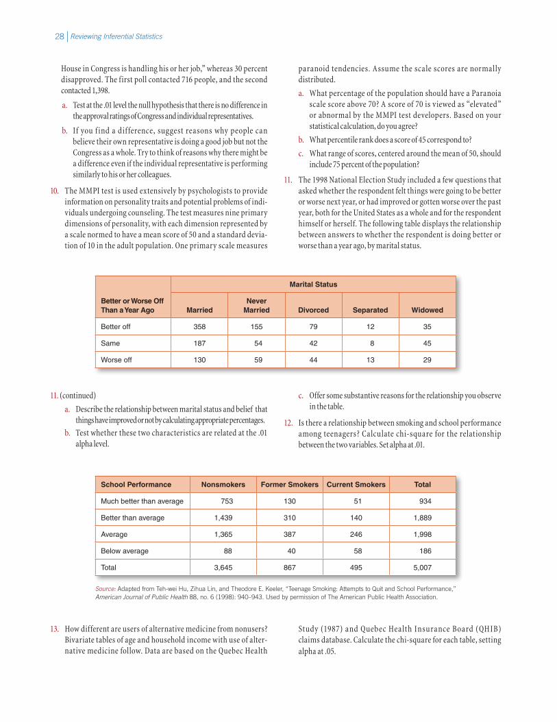
11. The 1998 National Election Study included a few questions that asked whether the respondent felt things were going to be better or worse next year, or had improved or gotten worse over the past year, both for the United States as a whole and for the respondent himself or herself. The following table displays the relationship between answers to whether the respondent is doing better or worse than a year ago, by marital status.

Better or Worse Off Than a Year Ago

Marital Status

MarriedNever

Married Divorced Separated Widowed

Better off 358 155 79 12 35

Same 187 54 42 8 45

Worse off 130 59 44 13 29

11. (continued)

a. Describe the relationship between marital status and belief that things have improved or not by calculating appropriate percentages.

b. Test whether these two characteristics are related at the .01 alpha level.

c. Offer some substantive reasons for the relationship you observe in the table.

12. Is there a relationship between smoking and school performance among teenagers? Calculate chi-square for the relationship between the two variables. Set alpha at .01.

School Performance Nonsmokers Former Smokers Current Smokers Total

Much better than average 753 130 51 934

Better than average 1,439 310 140 1,889

Average 1,365 387 246 1,998

Below average 88 40 58 186

Total 3,645 867 495 5,007

Source: Adapted from Teh-wei Hu, Zihua Lin, and Theodore E. Keeler, “Teenage Smoking: Attempts to Quit and School Performance,” American Journal of Public Health 88, no. 6 (1998): 940–943. Used by permission of The American Public Health Association.

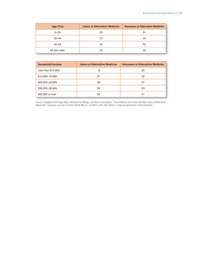
13. How different are users of alternative medicine from nonusers? Bivariate tables of age and household income with use of alter-native medicine follow. Data are based on the Quebec Health

Study (1987) and Quebec Health Insurance Board (QHIB) claims database. Calculate the chi-square for each table, setting alpha at .05.


Age (Yrs) Users of Alternative Medicine Nonusers of Alternative Medicine

0–29 39 51

30–44 72 44

45–64 42 52

65 and older 16 22

Household Income Users of Alternative Medicine Nonusers of Alternative Medicine

Less than $12,000 8 30

$12,000–19,999 27 22

$20,000–29,999 38 37

$30,000–39,999 26 23

$40,000 or over 53 41

Source: Adapted from Regis Blais, Aboubacrine Maiga, and Alarou Aboubacar, “How Different Are Users and Non-users of Alternative Medicine?” Canadian Journal of Public Health 88, no. 3 (1997): 159–162, Table 1. Used by permission of the publisher.

reviewing inferential statistics

Documents