REVISED VERSION 1

Detecting Changes in the EnvironmentBased on Full Posterior Distributions

over Real-valued Grid MapsLukas Luft, Alexander Schaefer, Tobias Schubert, Wolfram Burgard

Abstract—To detect changes in an environment, one has todecide whether a set of observations is incompatible with a setof previously made observations. For binary, lidar-based gridmaps, this is essentially the case when the laser beam traverses avoxel which has been observed as occupied, or when the beam isreflected by a voxel which has been observed as empty. However,due to discretization errors, some voxels are neither completelyoccupied nor completely free. These voxels have to be modeled byreal-valued variables, whose estimation is an inherently statisticalprocess. Thus, it is nontrivial to decide whether two sets ofobservations emerge from the same underlying true map values,and hence from an unchanged environment. Our main idea isto account for the statistical nature of the estimation process byleveraging the full map posteriors instead of only the most likelymaps. Closed-form solutions of posteriors over real-valued gridmaps have been introduced recently. We leverage a similaritymeasure on these posteriors to calculate for each point in timethe probability that it constitutes a change in the hidden mapvalue. While the proposed approach works for any type of real-valued grid map that allows the computation of the full posterior,we provide all formulas for the well-known reflection mapsand the recently introduced decay-rate maps. We introduce andcompare different similarity measures and show that our methodsignificantly outperforms baseline approaches in simulated andreal world experiments.

Index Terms—Mapping, range sensing

I. INTRODUCTION

Grid maps are a popular approach in the context of mobilerobots to represent the environment. Their key idea is topartition the environment into discrete voxels, where eachvoxel stores a particular value related to a specific propertyof the environment in the corresponding location. Lidarsare a popular sensor for building such maps due to theiraccuracy. They send out laser beams and measure the timethe beams need to return after being reflected from objects inthe environment.

Typically, environments exhibit temporary or permanentchanges, which the robot has to detect and react to. Consideroccupancy grid maps, in which each cell is either free oroccupied. Here, observing a reflection in a free cell or a trans-mission through an occupied cell is an indication of a changein the environment. However, reasoning about these changes

This work has been partially supported by the EuropeanCommission in the Horizon 2020 framework program under grantagreements 644227-Flourish and 645403-RobDREAM, by theGraduate School of Robotics in Freiburg, and by the State GraduateFunding Program of Baden-Wurttemberg. All authors are with theDepartment of Computer Science, University of Freiburg, Germany.{luft,aschaef,tobschub,burgard}@cs.uni-freiburg.de

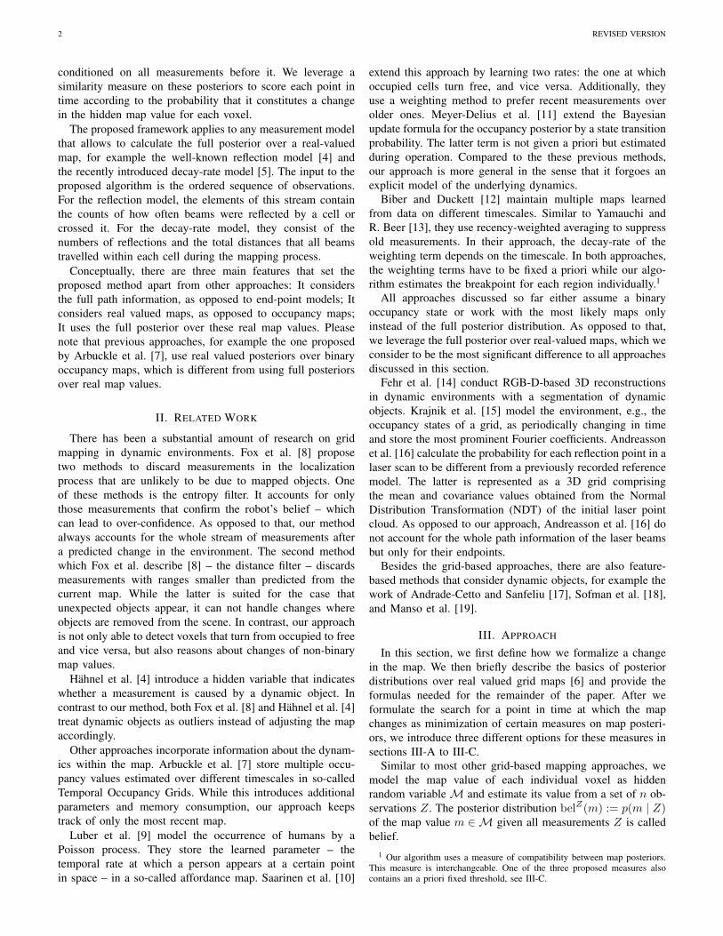
Fig. 1: Exemplary views of the changing environment in whichwe conduct one of our mapping experiments.

is more complicated in real-world applications, where cells arenot always completely free or occupied. These types of cellsare required to represent semi-transparent objects, structuressmaller than the voxel size, or glass. To model the stochasticbehavior of a beam within such a voxel, one has to use real-valued maps. Their values can either be interpreted as occu-pancy probabilities [1], [2], [3], reflection probabilities [4],or as expected laser ray lengths [5]. It is non-trivial to decidewhether a set of observations is within stochastic fluctuation ordue to an actual change in the environment. This is particularlytrue if the map representation only comprises the most likelyvalues, as opposed to the full posterior distributions. Consider,for example, a set of observations within a voxel, most ofwhich report a reflection. Only with a notion of uncertaintyabout a previously estimated map value, one can judge whetherthe observations are likely to be in accordance with this value.

Our main idea is that if the full map posteriors are given,we can score pairs of temporary maps conditioned on distinctsets of observations according to their compatibility. To getthe map posteriors we apply mapping with known poses. Luftet al. [6] recently introduced closed-form solutions to the fullmap posteriors over real-valued maps. For each point in time,this approach computes two posteriors, the one conditionedon all measurements after this point in time and the one

2 REVISED VERSION

conditioned on all measurements before it. We leverage asimilarity measure on these posteriors to score each point intime according to the probability that it constitutes a changein the hidden map value for each voxel.

The proposed framework applies to any measurement modelthat allows to calculate the full posterior over a real-valuedmap, for example the well-known reflection model [4] andthe recently introduced decay-rate model [5]. The input to theproposed algorithm is the ordered sequence of observations.For the reflection model, the elements of this stream containthe counts of how often beams were reflected by a cell orcrossed it. For the decay-rate model, they consist of thenumbers of reflections and the total distances that all beamstravelled within each cell during the mapping process.

Conceptually, there are three main features that set theproposed method apart from other approaches: It considersthe full path information, as opposed to end-point models; Itconsiders real valued maps, as opposed to occupancy maps;It uses the full posterior over these real map values. Pleasenote that previous approaches, for example the one proposedby Arbuckle et al. [7], use real valued posteriors over binaryoccupancy maps, which is different from using full posteriorsover real map values.

II. RELATED WORK

There has been a substantial amount of research on gridmapping in dynamic environments. Fox et al. [8] proposetwo methods to discard measurements in the localizationprocess that are unlikely to be due to mapped objects. Oneof these methods is the entropy filter. It accounts for onlythose measurements that confirm the robot’s belief – whichcan lead to over-confidence. As opposed to that, our methodalways accounts for the whole stream of measurements aftera predicted change in the environment. The second methodwhich Fox et al. describe [8] – the distance filter – discardsmeasurements with ranges smaller than predicted from thecurrent map. While the latter is suited for the case thatunexpected objects appear, it can not handle changes whereobjects are removed from the scene. In contrast, our approachis not only able to detect voxels that turn from occupied to freeand vice versa, but also reasons about changes of non-binarymap values.

Hahnel et al. [4] introduce a hidden variable that indicateswhether a measurement is caused by a dynamic object. Incontrast to our method, both Fox et al. [8] and Hahnel et al. [4]treat dynamic objects as outliers instead of adjusting the mapaccordingly.

Other approaches incorporate information about the dynam-ics within the map. Arbuckle et al. [7] store multiple occu-pancy values estimated over different timescales in so-calledTemporal Occupancy Grids. While this introduces additionalparameters and memory consumption, our approach keepstrack of only the most recent map.

Luber et al. [9] model the occurrence of humans by aPoisson process. They store the learned parameter – thetemporal rate at which a person appears at a certain pointin space – in a so-called affordance map. Saarinen et al. [10]

extend this approach by learning two rates: the one at whichoccupied cells turn free, and vice versa. Additionally, theyuse a weighting method to prefer recent measurements overolder ones. Meyer-Delius et al. [11] extend the Bayesianupdate formula for the occupancy posterior by a state transitionprobability. The latter term is not given a priori but estimatedduring operation. Compared to the these previous methods,our approach is more general in the sense that it forgoes anexplicit model of the underlying dynamics.

Biber and Duckett [12] maintain multiple maps learnedfrom data on different timescales. Similar to Yamauchi andR. Beer [13], they use recency-weighted averaging to suppressold measurements. In their approach, the decay-rate of theweighting term depends on the timescale. In both approaches,the weighting terms have to be fixed a priori while our algo-rithm estimates the breakpoint for each region individually.1

All approaches discussed so far either assume a binaryoccupancy state or work with the most likely maps onlyinstead of the full posterior distribution. As opposed to that,we leverage the full posterior over real-valued maps, which weconsider to be the most significant difference to all approachesdiscussed in this section.

Fehr et al. [14] conduct RGB-D-based 3D reconstructionsin dynamic environments with a segmentation of dynamicobjects. Krajnik et al. [15] model the environment, e.g., theoccupancy states of a grid, as periodically changing in timeand store the most prominent Fourier coefficients. Andreassonet al. [16] calculate the probability for each reflection point in alaser scan to be different from a previously recorded referencemodel. The latter is represented as a 3D grid comprisingthe mean and covariance values obtained from the NormalDistribution Transformation (NDT) of the initial laser pointcloud. As opposed to our approach, Andreasson et al. [16] donot account for the whole path information of the laser beamsbut only for their endpoints.

Besides the grid-based approaches, there are also feature-based methods that consider dynamic objects, for example thework of Andrade-Cetto and Sanfeliu [17], Sofman et al. [18],and Manso et al. [19].

III. APPROACH

In this section, we first define how we formalize a changein the map. We then briefly describe the basics of posteriordistributions over real valued grid maps [6] and provide theformulas needed for the remainder of the paper. After weformulate the search for a point in time at which the mapchanges as minimization of certain measures on map posteri-ors, we introduce three different options for these measures insections III-A to III-C.

Similar to most other grid-based mapping approaches, wemodel the map value of each individual voxel as hiddenrandom variableM and estimate its value from a set of n ob-servations Z. The posterior distribution belZ(m) := p(m | Z)of the map value m ∈M given all measurements Z is calledbelief.

1 Our algorithm uses a measure of compatibility between map posteriors.This measure is interchangeable. One of the three proposed measures alsocontains an a priori fixed threshold, see III-C.

LUFT et al.: DETECTING CHANGES 3

Let us assume that the environment changes at some point intime (let us call it a breakpoint b) because an object is removedor added. Then, instantly, the hidden variables correspondingto voxels that are affected by this change are replaced by newvariables. For the voxels in question, all measurements takenbefore the breakpoint bias the estimate of the new randomvariable. Thus, for a potential breakpoint, we define twodistributions: the map posterior bel1:b−1 conditioned on themeasurements before the breakpoint and the posterior belb:n

conditioned on the recent measurements from the breakpointon. If the robot has to localize itself, it must use the mostrecent map. Thus, it is desirable to detect the breakpoint band maintain belb:n.

Luft et al. [6] show that, for two particular measurementmodels, the beliefs over individual non-binary map valuescan be parametrized as follows. The well-known reflectionmodel [4] assigns to each voxel a reflection probability µ.Given the hidden map value µ, the likelihood to observe aparticular stream Z of observations with H reflections (hits)and M transmissions (misses) in the cell is

Lµ(Z) := p(Z | µ) = µH (1− µ)M. (1)

The map posteriors are beta-distributions [6]

bel(µ) = Beta(µ;α, β) =µα−1(1− µ)β−1

B(α, β), (2)

with the beta function B(·, ·). The parameters α and β aredetermined by the number of reflections and transmissions:α = H + α0 and β = M + β0, where α0 and β0 are priorsand α0 = β0 = 1 for a uniform prior. The recently introduceddecay-rate model [5] assigns each voxel a decay-rate λ. Here,the likelihood for a stream Z with H reflections and all laserbeams travel a total distance R within the cell is

Lλ(Z) := p(Z | λ) = λH exp (−λR) . (3)

The map posteriors are gamma-distributions [6]

bel(λ) = Gamma(λ;α, β) =βα

Γ(α)λα−1e−βλ, (4)

with the gamma function Γ(·), α = H + α0, β = R+ β0,where α0 = 1 and β0 = 0 for an uninformed prior.

Please note that in their original formulation [1], [2], [3],occupancy grid maps possess binary map values, such thatthe map posterior for each voxel is a Bernoulli distribution,represented by one real value p. As opposed to that, for thetwo map representations introduced in this section, the mapvalues are already real numbers, such that the posterior foreach voxel is a continuous distribution.

Based on the parametrized posteriors, the aim of this paperis to formalize a criterion that allows a breakpoint detection.We are looking for a measure M such that the expectedbreakpoint b∗ is

b∗ = argminb∈B

M(

bel1:b−1,belb:n), (5)

where B ⊂ N≤n is a set of potential breakpoints. Please notethat b∗ = 1 means that we detect that the environment didnot change. We ensure that 1 ∈ B, where bel1:0 = bel∅

is a prior distribution. To associate each of the collectedmeasurements to either bel1:b−1 or belb:n we have to preservetheir temporal order. However, the order between potentialbreakpoints can be neglected to the benefit of reduced memoryusage, which is particularly relevant for |B| � n. This appliesfor lidars that see a voxel multiple times within one scanalmost simultaneously, assuming that a breakpoint can onlyoccur between individual scans. Therefore, in our real-worldexperiments IV-B, we define the potential breakpoints to liebetween individual scans. Depending on the concrete use case,one can choose the potential breakpoints substantially moresparsely. A service robot, for example, could check for break-points every time it revisits a particular room. Accordingly,it is sufficient to store the map generated during a particularvisit as a single measurement, instead of maintaining the entirestream of laser scans. Please note that our approach explicitlyassumes instantaneous changes of map values. This is no lossof generality, as one can choose the set of possible breakpointssuch that it fits the dynamics of the situation.

In principle, it is possible to apply our framework in anonline setting. Every time a new laser scan arrives, the mapposteriors are updated recursively and the values M in (5) haveto be recalculated. When a breakpoint is detected, all previousmeasurements can be deleted.

Thus far, we assumed that each voxel contains either asingle breakpoint or no breakpoints at all. However, in manyapplications the robot might face multiple changes withinindividual voxels during its mission. Ideally, these breakpointsmanifest as local minima in the objective function M in (5).The experiments in Section IV-A indicate that our methodcan also deal with multiple breakpoints. However, it is subjectof future research to take these multiple breakpoints moreexplicitly into account.

In the remainder of this section, we discuss three differentoptions for the measure M in (5).

A. Bayesian Information Criterion

A natural choice for M is the Bayesian Information Crite-rion (BIC) [20]

BIC = ln (n) k − 2 ln(L), (6)

with the number of measurements n, the number of parametersin the model k, and the maximized measurement likelihoodL. The first term penalizes over-fitting, while the second termrewards the goodness of fit.

For b = 1, we assume that we only have one map value.Then, the likelihood function for the reflection model is givenby (1) and the likelihood for the decay-rate model is given by(3). These likelihoods both possess only a single parameter,namely µ or λ, respectively. Thus, we set k = 1 in (6). If weassume two posteriors – one conditioned on the measurementsbefore b and the other conditioned on the measurements after– we have k = 3. The parameters are the breakpoint b and themap values of both posteriors. For the reflection model, thelikelihood term can thus be calculated from (1) as

L = Lµ1:b−1

(Z1:b−1)Lµb:n

(Zb:n

),

4 REVISED VERSION

with the maximum likelihood parameters

µ1:b−1 = H1:b−1(H1:b−1 +M1:b−1)−1

and µb:n accordingly [6]. For the decay-rate model, the like-lihood term can be calculated from (3) as

L = Lλ1:b−1

(Z1:b−1)Lλb:n

(Zb:n

),

with the maximum likelihood parameters

λ1:b−1 = H1:b−1(R1:b−1)−1

and λb:n accordingly [6].Please note that the map posteriors are sufficient to calcu-

late (6). Thus, minimizing the BIC is a special case of (5).If the minimum is attained at b = 1, the BIC-based methodimplies that there is no change in the environment.

In the following, we introduce two measures that considerthe full map posteriors in contrast to the BIC, which onlyaccounts for the measurement likelihood given the most likelymap parameters,

B. Entropy-based approach

As a second option for M we introduce an entropy-basedapproach. We assume that the entropy of a posterior distri-bution with given parameterization generally decreases withthe number of measurements. This is implies that if theincorporation of an additional set of measurements leads toan increase of the entropy, this set must be generated from adifferent random variable. Thus we are looking for the set ofmost recent measurements that minimize the entropy

b∗ = argminb∈B

H(

belb:n). (7)

For the reflection model, the posterior belb:n is a Beta distri-bution. Its entropy is

H [Beta(α, β)] = ln [B(α, β)] + (α+ β − 2)ψ(α+ β)

− (α− 1)ψ(α)− (β − 1)ψ(β)

with the digamma function ψ(·) and the beta function B(·, ·).For the decay-rate model, the posterior belb:n is a Gammadistribution with entropy

H [Gamma(α, β)] =α+ ln

(Γ(α)

β

)+ (1− α)ψ(α)

where Γ(·) is the gamma function.Please note that in the case of binary occupancy grids,

the entropy of the posterior is minimal for the Bernoulliparameters p = 0 or p = 1. Thus, the entropy-based approachalways maintains the latest stream of observations whichcontains either only hits or only misses. As this will lead tosevere over-confidence, it is essential to leverage the posteriorsover real-valued maps.

C. Probabilistic approach

In addition to the BIC, which considers the most likely mapparameters, and the entropy-based approach, which accountsfor the full map posterior conditioned on the measurementsafter a potential breakpoint, we now introduce a new measure,which compares two map posteriors. Therefor, we analyt-ically derive the probability density Pb that two posteriordistributions bel1:b−1 and belb:n are generated from the sameunderlying random variable:

Pb :=

∫m

∫m′

bel1:b−1(m) belb:n(m′)δ(m−m′)dmdm′

=

∫m

bel1:b−1(m) belb:n(m)dm. (8)

We assume that the probability for both distributions tobe generated by the same hidden variable is minimal at thebreakpoint. Thus

b∗ = argminb∈B

Pb

(bel1:b−1,belb:n

). (9)

For the reflection model, the objective function reduces to

Pb =

∫ 1

0

Beta(µ;α1:b−1, β1:b−1)Beta

(µ;αb:n, βb:n

)dµ

=

∫ 1

0

µα1:b−1−1(1− µ)β

1:b−1−1

B(α1:b−1, β1:b−1)

µαb:n−1(1− µ)β

b:n−1

B(αb:n, βb:n)dµ

=

∫ 1

0

µα1:b−1+αb:n−2(1− µ)β

1:b−1+βb:n−2

B(α1:b−1, β1:b−1) B(αb:n, βb:n)dµ

=

∫ 1

0

Beta(µ;α1:b−1 + αb:n − 1, β1:b−1 + βb:n − 1)dµ

· B(α1:b−1 + αb:n − 1, β1:b−1 + βb:n − 1)

B(α1:b−1, β1:b−1) B(αb:n, βb:n)

=B(α1:b−1 + αb:n − 1, β1:b−1 + βb:n − 1)

B(α1:b−1, β1:b−1) B(αb:n, βb:n)(10)

For the decay-rate model, we replace the beta distributions bygamma distributions and integrate from zero to infinity. Witha similar derivation as in (10), we get

Pb =

(β1:b−1

β1:b−1 + βb:n

)α1:b−1 (βb:n

β1:b−1 + βb:n

)αb:n

· (β1:b−1 + βb:n)

(α1:b−1 + αb:n − 1) B(α1:b−1, αb:n)(11)

Please note that Pb is a particular value of a probabilitydensity function. To determine the value P1 from (8), one hasto define bel∅. In our experiments, we treat P1 as a fixedparameter and determine it via cross-validation, as explainedin Section IV-A.

It is straightforward to apply the metric (8) to binaryoccupancy maps where m ∈ {0, 1}. Here, the real value µis the occupancy probability and hence represents the fullposterior. Replacing the integral in (8) by a sum, yields

Pb = µ1:b−1µb:n +(1− µ1:b−1) (1− µb:n) . (12)

Here, Pb is a probability, as opposed to the probability densityfunction in the case of the real-valued maps. A natural choiceof the prior µ∅ = 0.5 results in P1 = 0.5.

LUFT et al.: DETECTING CHANGES 5

IV. EXPERIMENTS

To evaluate our method, we perform experiments in simu-lation and with a real-world dataset. In the experiments, wecompare the following approaches• TRUE: uses the true breakpoint.• BIC: the Bayesian Information Criterion III-A.• ENT: the entropy-based approach III-B.• PRO: the probabilistic approach III-C.• BIN: the probabilistic approach on binary maps (12).• NDT: the NDT-based approach [16].• BASE: the baseline that assumes a static environment

(b = 1).Note that TRUE is the map generated from all mea-

surements after the true (typically unknown) breakpoint. Wecompare our method against NDT as presented by Andrea-son et al. [16]. It generates a reference model of the initialenvironment represented by the Normal Distribution Transfor-mation of the corresponding point cloud. For each point inthe subsequent laser scans, it computes the probability to bedifferent from this reference model.

A. Simulation experiments

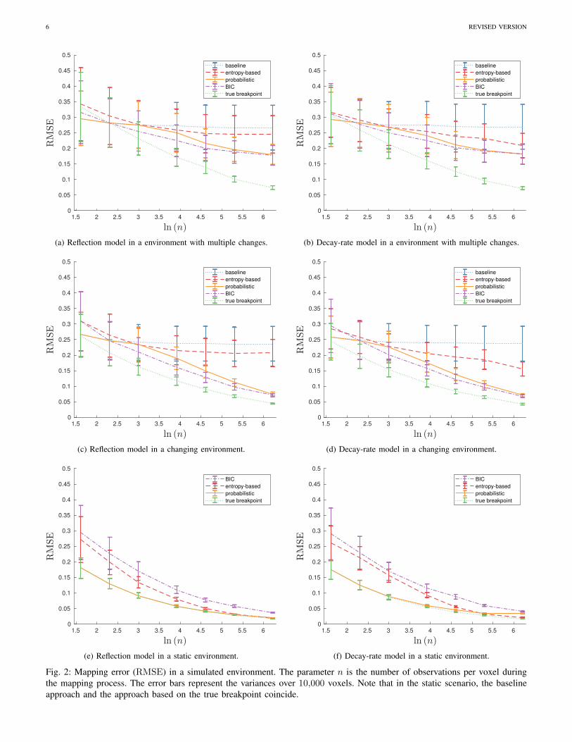
We perform an experiment with randomly chosen groundtruth map values and simulated lidar observations as follows.We consider an environment of N = 104 voxels. A robot visitsevery voxel n times and collects the measurements H , M , andR. We simulate these measurements according to randomlygenerated ground truth map values µ and λ. For each cell, wedraw µ and Pref := 1− exp(−λ · l) with l = 1m from a uni-form distribution over [0, 1].2 To simulate changes in the map,these true map values change after a breakpoint b. For eachvoxel, we draw b from a uniform distribution over {1, . . . , n}.For each voxel, we estimate the breakpoint based on thedifferent approaches and use the stream of all measurementsfrom b on to generate the map posterior. We repeat the wholeexperiment for n ∈ {5, 10, 20, 50, 100, 200, 500}. Figs. 2cand 2d show the root mean squared error per voxel (RMSE)between the maps estimated by the different approaches andthe true map. For the decay-rate maps, we compare Prefinstead of λ.

The algorithm produces a false positive if it detects abreakpoint where the true map value remains the same. Thesefalse positives are particularly adverse in static environments,where a false breakpoint detection reduces the number ofmeasurements taken into account for mapping. The situationmost prone to false positives is when all map values areconstant. The results are shown in Figs. 2e and 2f. Note thatin this case the baseline approach coincides with the approachbased on the true breakpoint.

To illustrate our intuition that the proposed algorithm canalso handle multiple changes within one voxel, we run thesimulation again with multiple breakpoints per voxel. For each

2In case of the decay-rate model, the map values λ can vary from zeroto infinity. Therefore, we transform λ into the interval [0, 1] by the formulaPref = 1−exp(−λ·l). Here, Pref can be interpreted as the probability thata perpendicularly incident laser beam is reflected within a voxel with valueλ and edge length l.

voxel, we draw the number of breakpoints from a uniformdistribution over the integers one to five. The correspondingresults are shown in Figs. 2a and 2b.

Please note that the value P1, which we need for the proba-bilistic approach, cannot be directly computed from (8). In theexperiments, we determine it via cross-validation. Therefor, werun the whole simulation experiment including the changingand the stationary scenario for different values of P1. Wechoose the value of P1 that minimizes the total RMSE onthis training phase and conduct the evaluation in Fig. 2 on anindependent simulation.

For both measurement models and all approaches except forthe baseline, the error decreases with the number of collectedmeasurements. In the changing environment with the decay-rate model, we observe that BIC and PRO perform better thanENT. For the reflection model, this effect manifests only witha growing number of measurements (n > 20). We attributethis to the fact that the decay-rate model takes into accountthe real valued distances of beams within a voxel in additionto the integer hits and misses. Therefore, it contains moreinformation than the reflection model, which is particularlyrelevant for small n. Independent of the measurement model,the BIC performs poorly in the static environment, whilethe entropy-based approach performs poorly in the changingenvironment. The proposed probabilistic approach performswell in all simulated situations. In particular, it produces veryfew false positives and therefore shows a performance closeto the ground truth in the static environment.

B. Real-world experiments

To test our approach in the real world, we create a dataset ina hall with a static Velodyne HDL-64E lidar sensor. We recordthe scene 13 times with an average of 65 scans per run. Inbetween the scanning phases, we change the scene by addingand removing objects. Two of the sequences include movingpeople. Overall, we generate 169 scenarios by concatenatingevery pair of sequences, including the combinations of eachsequence with itself to simulate static scenes. For each sce-nario, we define the ground truth as the map generated fromthe second sequence of observations. Fig. 1 shows a typicalscene of the overall dataset.

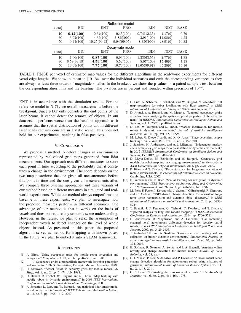
We search for breakpoints between each pair of laser scans.For P1 in (8), we use the cross-validation values from thesimulation runs. We compute the RMSE per voxel betweenthe map generated from TRUE and the maps calculated fromthe individual approaches. Since the majority of voxels doesnot change, BASE has a low error. To demonstrate that theindividual approaches outperform the baseline-approach, weconduct a one-tailed, paired-sample t-test. The p-values inTab. I correspond to the probability that the correspondingalgorithm produces a smaller error than the baseline approach.The variances of the RMSE over the individual scenariosare always three orders of magnitude smaller than the mean.With the proposed method, all three measures significantlyoutperform the baseline. For the decay-rate model, the entropy-based approach performs best. Considering that large regionsof the environment remain static, the good performance of

6 REVISED VERSION

1.5 2 2.5 3 3.5 4 4.5 5 5.5 60

0.05

0.1

0.15

0.2

0.25

0.3

0.35

0.4

0.45

0.5

baseline

entropy-based

probabilistic

BIC

true breakpoint

(a) Reflection model in a environment with multiple changes.

1.5 2 2.5 3 3.5 4 4.5 5 5.5 60

0.05

0.1

0.15

0.2

0.25

0.3

0.35

0.4

0.45

0.5

baseline

entropy-based

probabilistic

BIC

true breakpoint

(b) Decay-rate model in a environment with multiple changes.

1.5 2 2.5 3 3.5 4 4.5 5 5.5 60

0.05

0.1

0.15

0.2

0.25

0.3

0.35

0.4

0.45

0.5

baseline

entropy-based

probabilistic

BIC

true breakpoint

(c) Reflection model in a changing environment.

1.5 2 2.5 3 3.5 4 4.5 5 5.5 60

0.05

0.1

0.15

0.2

0.25

0.3

0.35

0.4

0.45

0.5

baseline

entropy-based

probabilistic

BIC

true breakpoint

(d) Decay-rate model in a changing environment.

1.5 2 2.5 3 3.5 4 4.5 5 5.5 60

0.05

0.1

0.15

0.2

0.25

0.3

0.35

0.4

0.45

0.5

BIC

entropy-based

probabilistic

true breakpoint

(e) Reflection model in a static environment.

1.5 2 2.5 3 3.5 4 4.5 5 5.5 60

0.05

0.1

0.15

0.2

0.25

0.3

0.35

0.4

0.45

0.5

BIC

entropy-based

probabilistic

true breakpoint

(f) Decay-rate model in a static environment.

Fig. 2: Mapping error (RMSE) in a simulated environment. The parameter n is the number of observations per voxel duringthe mapping process. The error bars represent the variances over 10,000 voxels. Note that in the static scenario, the baselineapproach and the approach based on the true breakpoint coincide.

LUFT et al.: DETECTING CHANGES 7

Reflection modell[cm] BIC ENT PRO BIN NDT BASE

10 0.42(100) 0.64(100) 0.45(100) 0.74(12.35) 1.17(0) 0.7030 3.92(100) 4.35(100) 3.86(100) 3.91(100) 11.08(0) 4.5550 9.44(100) 10.25(99.43) 9.94(99.95) 8.39(100) 28.91(0) 10.32

Decay-rate modell[cm] BIC ENT PRO BIN NDT BASE

10 1.00(100) 0.87(100) 0.93(100) 1.33(63.55) 2.77(0) 1.3530 6.53(99.99) 4.59(100) 5.52(100) 5.97(100) 15.40(0) 7.1550 13.03(100) 7.75(100) 10.73(100) 11.65(99.97) 35.28(0) 14.16

TABLE I: RMSE per voxel of estimated map values for the different algorithms in the real-world experiments for differentvoxel edge lengths. We show its mean in [10−4m] over the individual scenarios and omit the corresponding variances as theyare always at least three orders of magnitude smaller. In the brackets, we show the p-values of a paired sample t-test betweenthe corresponding algorithms and the baseline. The p-values are in percent and rounded within precision of 10−4.

ENT is in accordance with the simulation results. For thereference model in NDT, we use all measurements before thebreakpoint. Since NDT only considers the end points of thelaser beams, it cannot detect the removal of objects. In ourdatasets, it performs worse than the baseline approach as itassumes that the spatial distribution of points within differentlaser scans remains constant in a static scene. This does nothold for our experiments, resulting in false positives.

V. CONCLUSION

We propose a method to detect changes in environmentsrepresented by real-valued grid maps generated from lidarmeasurements. Our approach uses different measures to scoreeach point in time according to the probability that it consti-tutes a change in the environment. The score depends on thetwo map posteriors: the one given all measurements beforethis point in time and the one given all measurements after.We compare three baseline approaches and three variants ofour method based on different measures in simulated and real-world experiments. While our method always outperforms thebaseline in these experiments, we plan to investigate howthe proposed measures perform in different scenarios. Oneadvantage of our method is that it works on the basis ofvoxels and does not require any semantic scene understanding.However, in the future, we plan to relax the assumption ofindependent voxels to detect changes on the level of wholeobjects instead. As presented in this paper, the proposedalgorithm serves as method for mapping with known poses.In the future, we plan to embed it into a SLAM framework.

REFERENCES

[1] A. Elfes, “Using occupancy grids for mobile robot perception andnavigation,” Computer, vol. 22, no. 6, pp. 46–57, June 1989.

[2] ——, “Occupancy grids: a probabilistic framework for robot perceptionand navigation,” Ph.D. dissertation, Carnegie Mellon University, 1989.

[3] H. Moravec, “Sensor fusion in certainty grids for mobile robots,” AIMag., vol. 9, no. 2, pp. 61–74, July 1988.

[4] D. Hahnel, R. Triebel, W. Burgard, and S. Thrun, “Map building withmobile robots in dynamic environments,” in 2003 IEEE InternationalConference on Robotics and Automation. Proceedings, 2003.

[5] A. Schaefer, L. Luft, and W. Burgard, “An analytical lidar sensor modelbased on ray path information,” IEEE Robotics and Automation Letters,vol. 2, no. 3, pp. 1405–1412, 2017.

[6] L. Luft, A. Schaefer, T. Schubert, and W. Burgard, “Closed-form fullmap posteriors for robot localization with lidar sensors,” in IEEEInternational Conference on Intelligent Robots and Systems, 2017.

[7] D. Arbuckle, A. Howard, and M. Mataric, “Temporal occupancy grids:a method for classifying the spatio-temporal properties of the environ-ment,” in IEEE/RSJ International Conference on Intelligent Robots andSystems, vol. 1, 2002, pp. 409–414 vol.1.

[8] D. Fox, W. Burgard, and S. Thrun, “Markov localization for mobilerobots in dynamic environments,” Journal of Artificial IntelligenceResearch, vol. 11, pp. 391–427, 1999.

[9] M. Luber, G. Diego Tipaldi, and K. O. Arras, “Place-dependent peopletracking,” Int. J. Rob. Res., vol. 30, no. 3, Mar. 2011.

[10] J. Saarinen, H. Andreasson, and A. J. Lilienthal, “Independent markovchain occupancy grid maps for representation of dynamic environment,”in 2012 IEEE/RSJ International Conference on Intelligent Robots andSystems, Oct 2012, pp. 3489–3495.

[11] D. Meyer-Delius, M. Beinhofer, and W. Burgard, “Occupancy gridmodels for robot mapping in changing environments,” in Twenty-SixthAAAI Conference on Artificial Intelligence, 2012, pp. 2024–2030.

[12] P. Biber and T. Duckett, “Dynamic maps for long-term operation ofmobile service robots,” in Proceedings of Robotics: Science and Systems,Cambridge, USA, 2005.

[13] B. Yamauchi and R. Beer, “Spatial learning for navigation in dynamicenvironments,” IEEE Transactions on Systems, Man, and Cybernetics,Part B (Cybernetics), vol. 26, no. 3, pp. 496–505, Jun 1996.

[14] M. Fehr, F. Furrer, I. Dryanovski, J. Sturm, I. Gilitschenski, R. Siegwart,and C. Cadena, “TSDF-based change detection for consistent long-term dense reconstruction and dynamic object discovery,” in IEEEInternational Conference on Robotics and Automation, 2017, pp. 5237–5244.

[15] T. Krajnik, J. P. Fentanes, G. Cielniak, C. Dondrup, and T. Duckett,“Spectral analysis for long-term robotic mapping,” in IEEE InternationalConference on Robotics and Automation, 2014, pp. 3706–3711.

[16] H. Andreasson, M. Magnusson, and A. Lilienthal, “Has somethingchanged here? autonomous difference detection for security patrolrobots,” in IEEE/RSJ International Conference on Intelligent Robots andSystems, 2007, pp. 3429–3435.

[17] J. Andrade-Cetto and A. Sanfeliu, “Concurrent map building and lo-calization on indoor dynamic environments,” International Journal ofPattern Recognition and Artificial Intelligence, vol. 16, no. 03, pp. 361–374, 2002.

[18] B. Sofman, B. Neuman, A. Stentz, and J. A. Bagnell, “Anytime onlinenovelty and change detection for mobile robots,” Journal of FieldRobotics, vol. 28, no. 4.

[19] L. J. Manso, P. Nez, S. da Silva, and P. Drews-Jr, “A novel robust scenechange detection algorithm for autonomous robots using mixtures ofgaussians,” International Journal of Advanced Robotic Systems, vol. 11,no. 2, p. 18, 2014.

[20] G. Schwarz, “Estimating the dimension of a model,” The Annals ofStatistics, vol. 6, no. 2, pp. 461–464, 1978.